Dynamics of Majority Rule on Hypergraphs
Abstract
A broad range of dynamical systems involve multi-body interactions, or group interactions, which may not be encoded in traditional graphical structures. In this work, we focus on a canonical example from opinion dynamics, the Majority Rule, and investigate the possibility to represent and analyse the system by means of hypergraphs. We explore the formation of consensus and restrict our attention to interaction groups of size , in order to simplify our analysis from a combinatorial perspective. We propose different types of hypergraph models, incorporating modular structure or degree heterogeneity, and recast the dynamics in terms of Fokker-Planck equations, which allows us to predict the transient dynamics toward consensus. Numerical simulations show a very good agreement between the stochastic dynamics and theoretical predictions for large population sizes.
Keywords:
majority rule, consensus, higher-order, non-linear, networks, group dynamics, hypergraphsI Introduction
Opinion dynamics is concerned with the study of consensus formation in populations of interacting individuals. An important evolution of the field has been to consider the impact of the structure of the underlying social network on the dynamics Castellano et al. 2009. In contrast with mean-field approaches, where all the agents are essentially connected with each other, network-based approaches assume that the agents are located at the nodes of a network and that they are sparsely related by direct, binary connections through edges. A combination of these edges allows for indirect connections through the notion of path. A wide range of models have been proposed so as to capture the ways in which social interactions between agents affect opinion formation, through factors like peer pressure and conviction. Here, we will focus on the popular class of models where each node may be in one of two states, represented by the binary variables 0 and 1. These allow us to model opinions relating to questions with a “yes”/“no” answer, as in a referendum for instance, or “left”/“right” political choices, and find interesting connections with statistical physics models for spin dynamics.
The Voter Model (VM) is a prime example of such binary models Clifford and Sudbury 1973 and is defined as follows. At discrete times, an agent is chosen uniformly at random from the population. This agent then adopts the opinion of one of its randomly-chosen neighbours in the underlying network. This update is repeated ad infinitum, or until consensus is necessarily reached on a finite connected graph. Importantly, VM is linear and it is dyadic in nature given that pairwise interactions alone are sufficient to capture the dynamics of the system. It is well known that VM is solvable on regular lattice structures in arbitrary spatial dimensions Redner 2001. This is due to the fact that the average node state is conserved on degree-regular graphs. VM has also been shown to be conservative on heterogeneous networks Sood et al. 2008, allowing for significant analytical progress to be made in the study of the associated dynamics on a wide range of graph topologies.
However, real-world dynamics often exhibit nonlinear and non-conservative behaviour. An important non-conservative generalisation of VM is the so-called Majority Rule (MR) model Galam 2002; Krapivsky and Redner 2003 where, at each update event, we choose a group of agents from the population, where . These agents form the interaction group, and may be chosen uniformly at random (as in a mean-field scenario), or in a way that is constrained by the underlying network, as we discuss below. After an interaction group is formed, all of its agents simultaneously adopt the majority opinion in the group. When is odd, the majority opinion is always well defined. When is even, and a tie is observed between the opinions, the consensus is either decided randomly, or by introducing a bias for one opinion Friedman and Friedman 1985.
An important aspect of MR is that interactions take place in groups, motivated by the mechanism of peer pressure, which questions the adequacy of networks to encode the interactions between agents. Indeed the dynamical model is based on group interactions while the underlying network only encodes pairwise interactions, and there is thus no simple way to choose a group of agents, e.g. when , should they form a triangle, or simply form a path of length 2? This type of questioning has gained a lot of attention in recent years Lambiotte et al. 2019; Battiston et al. 2020, as it was observed that many systems exhibit multi-body or group interactions, such as in neural activity Giusti et al. 2015; Reimann et al. 2017; Santos et al. 2019, robotics Olfati-Saber et al. 2007 or scientific collaborations Patania et al. 2017, and that traditional graphical structures are incapable of reflecting the multi-body nature of such interactions. In order to circumvent this issue, a natural choice is to adopt a more general class of topological structures known as hypergraphs where interactions may, as the dynamical system, be multi-body. While there are other topological structures that are capable of encoding group interactions such as simplicial complexes Torres and Bianconi 2020 and bipartite graphs Newman et al. 2002, hypergraphs constitute a straightforward representation of multi-body interactions on networks, and appear to be an ideal candidate for the representation and analysis of MR dynamics Lanchier and Neufer 2013. Importantly, as shown in Neuhäuser et al. 2020, nonlinear multibody interactions are not expressible as linear combinations of pairwise interactions between adjacent nodes on a standard graph. MR dynamics on hypergraphs can thus not be reduced to a dynamics on standard networks in general.
The main purpose of this article is to investigate MR dynamics on a broad range of hypergraph models. For the sake of simplicity, we will restrict our attention to interaction groups of size , referred to as , even if most of our results could be generalised to general group size. In Section II, we start by reviewing results about the MR model in the mean-field limit, revealing its non-conservative nature and deriving some of its properties through a Fokker-Planck equation. In Section III, we then investigate MR dynamics on the so-called tripartite hypergraph, which is a natural generalisation of the mean field case where the system is made of 3 types of nodes. In Section IV, we consider a model of hypergraphs with community structure, referred to as modular hypergraphs, and then extend our analysis to heterogeneous hypergraphs in Section V. Section VI concludes our work.
II Mean-Field Analysis
II.1 Exact Analysis of the Exit Probability
The selection rule constitutes a key element of the MR model. We begin by considering the dynamics in the mean-field. The model is defined as follows. Each node is endowed with a binary state variable, denoted by 0 and 1. At each time step, agents are chosen uniformly at random and the Majority Rule is applied. This random selection can be formulated conveniently in the language of hypergraphs. Let us consider a fully connected hypergraph of agents. The hypergraph structure consists of the node set and, as we restrict ourselves to three-body interactions, the set of all possible triangles given by . The resulting object is a first generalisation of fully connected graphs to hypergraphs. The selection of a group of 3 nodes is now defined as the random selection of one hyperedge in the set of available hyperedges.
When studying the Majority Rule, as well as other opinion dynamics models with discrete states, an important quantity is the exit probability defined as follows. Suppose that the system is initialised with agents in the 1 state and agents in the 0 state. The exit probability is the probability that the system reaches consensus with all agents in the 1 state given that agents are initiated in the 1 state. Krapivsky and Redner Krapivsky and Redner 2003 adopted a combinatorial approach in deriving an exact expression for in the mean-field:
| (1) |
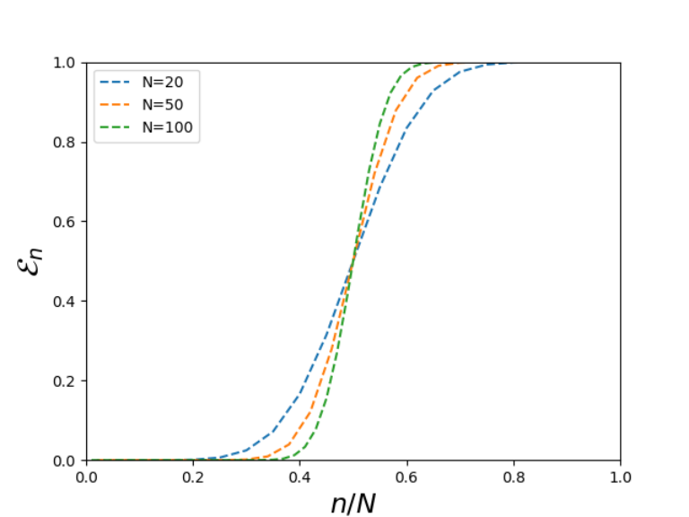
Figure 1 illustrates mean field exit probabilities using and agents. The initial fraction of agents in the 1 state is plotted on the -axis while the exit probability is plotted on the -axis. The exit probability is sigmoidal in nature, rapidly changing in a narrow interval centred at the pivotal value . As the exit probability converges to for Krapivsky and Redner 2003. In other words, the asymptotic mean-field exit probability is akin to a step function with discontinuity at . The complex functional form of is a manifestation of the nonlinear and non-conservative nature of MR interactions.
II.2 The Fokker-Planck Approach
We now go beyond the workings presented in Krapivsky and Redner 2003 and approach the mean-field analysis from a different perspective. In this section, we study the exit probability and the dynamical approach towards consensus in the asymptotic limit . Let denote the density of 1’s in the population at time ; that is, the fraction of agents in the 1 state at time . We shall write as for convenience, though the dependence in is implicit. Furthermore, let denote the incremental change in following an update event. We define the quantities to reflect the density of states in the population after an interaction takes place. Let and denote the raising and lowering operators Sood et al. 2008 that give the transition probabilities for the update events and respectively. Finally, let be the probability that the density of 1’s in the population is at time . The probability density evolves according to the following master equation over the incremental time period :
| (2) |
where and are assumed to denote and respectively. A conventional choice of the quantity is Chen and Redner 2005; Sood et al. 2008. We proceed by Taylor expanding the left hand side of equation (2) to first order in and the right hand side to second order in . This ultimately yields the Fokker-Planck equation:
| (3) |
In order to proceed, it is instructive to highlight the connection between equation (3) and its associated stochastic differential equation. Suppose that is a stochastic process on the sample space over the time interval for some , whose stochastic differential is given by
| (4) |
where is a standard Brownian motion. and are referred to as the drift and diffusion coefficients respectively. We shall also refer to as the drift velocity. The Fokker-Planck equation associated with the probability density of the random variable is given by
| (5) |
where . Comparing equations (3) and (5) we observe that the density may be described as a stochastic process with drift velocity and diffusion coefficient defined as follows:
| (6) | ||||
| (7) |
If is sufficiently large so that , equations (6) and (7) simplify to give
| (8) | ||||
| (9) |
Equations (8) and (9) illustrate that the drift velocity is whereas the diffusion term is . The drift velocities thus dominate the dynamics of the system for sufficiently large , as diffusive contributions vanish in the asymptotic limit. This observation will underpin much of the analysis presented throughout the course of this paper.
In the absence of diffusive contributions, we can use equation (4) to write , and thus integrate equation (8) directly to give the following result:
where . This indicates that the system will rapidly reach consensus with all agents in the 0 state if . Conversely, if then the system will reach consensus with all agents in the 1 state. As a validation of our results, we simulate the mean-field MR dynamics in a population of size . Figure 2 shows two representative results with . The density profiles are analogous for with a reflection in the line . The analytical trajectory is plotted in red, while the stochastic trajectory is plotted in blue. The time scale on the -axis is measured in units of Monte Carlo steps per node, so that . The trajectories are in excellent agreement when the initial value is sufficiently far from , and the system rapidly approaches consensus along the predicted trajectories. When where , however, diffusive fluctuations at early times can lead to a temporal shift in the density profile along the -axis, and deviations between the predictions and the stochastic simulations can be observed, as illustrated in Figure 2(a). Such diffusive effects become negligible as .
III The Tripartite Hypergraph
In this Section we move beyond the mean-field and consider hypergraphs with more sophisticated topologies. A natural starting point in this regard is the tripartite hypergraph, denoted by . The tripartite hypergraph consists of three distinct groups of nodes, which we shall refer to as , , and . We assume for the sake of simplicity that each group consists of agents. Let and denote the sets of nodes in groups , and respectively. Let us define the set of triangles on as . In other words, we consider all possible triplets with one agent in each group, hence generalising the notion of the complete bipartite graph. As before, at each step, a group of 3 nodes is chosen by selecting one hyperedge in at random.
Let us now adapt our treatment of the mean-field via a Fokker-Planck equation to this setting. Let denote the density of nodes in state 1 in at time , and let denote the change in resulting from the changing of opinion of a single agent in . We then define . Analogous expressions hold for agents in and where and denote the associated densities of 1’s respectively. We also define the raising and lowering operators associated with , denoted by and respectively (written as and for convenience). is the transition probability associated with the update event , whereas is the transition probability associated with the update event . Once again, analogous expressions exist for the raising and lowering operators associated with groups and . and are given as follows:
| (10) | ||||
| (11) |
Equation (10) follows from the fact that increases to if we choose a node in state 0 from as well as two nodes in state 1 from and . Similarly, equation (11) is derived from the fact that decreases to if we choose a node in state 1 from as well as two nodes in state 0 from and . The same logic applies for the calculation of the transition probabilities for groups and .
Using these transition probabilities we can deduce the probabilistic master equation governing MR dynamics on the tripartite hypergraph, where is the probability of the system having densities and at time :
| (12) |
We proceed by Taylor expanding the left hand side of equation (12) to first order in and the right hand side to second order in and . We take to be equal to the reciprocal of the total number of nodes in the hypergraph, in line with the convention introduced in Section II. This ultimately yields the three-dimensional Fokker-Planck equation:
| (13) |
As in the mean field case, it is instructive to highlight the connection between equation (13) and its corresponding stochastic differential equation. Consider an -dimensional stochastic process on the time interval and the sample space , where and . Suppose has stochastic differential
| (14) |
where is an -dimensional random vector, is an dimensional matrix and is a standard -dimensional Weiner process where . If we denote the probability density associated with the stochastic process by , then obeys the following Fokker-Planck equation:
| (15) |
where is the vector of drift velocities and is the diffusion tensor. Let us denote the drift velocity associated with the density of 1’s in by and the corresponding diffusion term by .
By comparing equations (13) and (15) we can deduce the following expressions:
| (16) | ||||
| (17) |
Note that in this instance the diffusion tensor is diagonal, where , and are equal to , and respectively. This is because we are considering interaction groups of size , meaning that only one of the quantities , or is varied at each update event. This is inherent in the structure of equation (12). Analogous expressions exist for the drift and diffusion terms for and . As in the mean field case, we note that the drift velocity is whereas the diffusive term is . This implies that the dynamics are dominated by the drift velocities for large , given that the diffusive contributions become negligible as . Using this fact, we posit that the dynamics of the system may be well approximated by discarding the diffusive terms and formulating a dynamical system using the drift velocities alone. This approach follows from the fact that in the absence of diffusive contributions, equation (14) reduces to a system of ordinary differential equations:
This system may be analysed via linear stability analysis. The set of fixed points is given by . When evaluated at the points and the eigenvalues of the Jacobian are with multiplicity , indicating asymptotic stability. When evaluated at the eigenvalues of the Jacobian are with multiplicity and with multiplicity . This implies that is a saddle point.
We investigate the performance of our model by conducting simulations on a tripartite hypergraph of nodes. Let us denote the initial conditions by . Figure 3 illustrates a sample set of simulation results with . The trajectory predicted by our deterministic nonlinear system is plotted in red, whereas the stochastic trajectory resulting from simulating the MR dynamics is plotted in blue. Given that the dynamical system is three-dimensional, it is informative to study the projections of the resultant trajectories in the and planes. These projections are plotted from left to right in Figure 3. The deterministic and stochastic trajectories are evidently in excellent agreement. This serves to validate our conjecture that the drift velocities dominate the dynamics of the system for large values of .
Our numerical simulations thus far have only focused on a specific trajectory of the dynamics resulting from an arbitrary choice of initial condition. We now extend our analysis by approximating the exit probability of the system for large ; that is, the probability that all of the agents reach consensus in the 1 state if the initial conditions are given by . In order to proceed, we consider the unstable fixed point at . The eigenvectors of the Jacobian when evaluated at this point are mutually orthogonal. The unstable linear subspace is spanned by the vector , which is normal to the surface of the stable linear subspace spanned by the remaining two eigenvectors. It is straightforward to deduce that the equation of the plane corresponding to the stable linear subspace is given by
| (18) |
By symmetry we posit that in the limit of large , the exit probability is given by the following piecewise function:
| (19) |
In order to confirm this prevision numerically, we vary and while keeping fixed. Figure 4 gives the simulation results for and , where . These plots were generated by initialising the stochastic dynamics at each point on the grid with uniform mesh size . Purple indicates consensus in the 0 state whereas yellow indicates consensus in the 1 state. The red dashed line marks the boundary predicted by equation (18) at . Only one simulation of the stochastic dynamics was conducted per coordinate, giving rise to diffusive effects at the interface separating the two domains. Nevertheless, the deterministic exit probability is in excellent agreement with the stochastic simulations of the system.
IV The Modular Hypergraph
IV.1 The Symmetric Case
In this Section we consider MR dynamics on hypergraphs with community structure, otherwise known as modular hypergraphs Kumar et al. 2018; Chodrow and Mellor 2020. In our setting, the population is partitioned into a number of non-overlapping sets known as modules or communities Newman 2006; Blondel et al. 2008. The modular hypergraph consists of two sets of nodes, referred to as communities and respectively. Let and denote the node sets in communities and respectively. The set of triangles on is defined as . In order to distribute the triangles over the hypergraph, we define the parameter which gives the probability of forming a triangle with agents in A and agents in . It follows that . These can be interpreted as hyperedge selection probabilities. Here, the hypergraph is assumed to be symmetric, meaning and . The total number of triangles is given by
In order to vary the degree to which the two components of the modular hypergraph interact, we introduce a parametric dependence inspired by the study of VM dynamics on the two-clique graph Sood et al. 2008. In graphical terms, communities and may be thought of as two fully-connected cliques of nodes. We then define an interconnectivity parameter such that each node in clique is, on average, connected to nodes in clique and vice versa. It follows that the average degree of a node in the graphical representation is , as each clique is complete. Using this graphical representation it is straightforward to calculate hyperedge selection probabilities:
| (20) | ||||
| (21) |
These probabilities satisfy normalisation. When it follows that while , hence the two modules evolve independently. Conversely, when it follows that whereas , corresponding to a mean-field of agents. We now define as the number of hyperedges with nodes in and nodes in . Using the fact that the hyperedge distribution may be determined as a function of :
| (22) | ||||
| (23) |
Note that hyperedges may have multiplicity greater than . This is due to the fact that the total number of hyperedges is fixed, regardless of the value of . For example, when we find that whereas . However, there are only ways to choose a hyperedge of size from nodes, implying that all hyperedges have multiplicity in this instance. This combinatorial consequence is immaterial to the dynamics of the system.
Once again, each agent in the population is assumed to occupy one of two states, labelled 0 and 1. Simulations are conducted using the hyperedge selection probabilities given in equations (20) and (21). This is equivalent to choosing hyperedges uniformly at random from the hyperdegree distribution given by equations (22) and (23). Let us denote the density of nodes in state 1 in and at time by and respectively. We write as and as for convenience. Let and where and . Let and be the raising operators that give the transition probabilities from and to and respectively. Similarly, let and be the lowering operators that give the transition probabilities from and to and respectively. and are given by
| (24) | ||||
| (25) |
Analogous expression exist for the operators and . Let be the probability that communities and have densities and respectively at time . Its associated master equation is given by
| (26) |
where . Taylor expanding the left hand side of equation (IV.1) to first order in and the right hand side to second order in and yields the following Fokker-Planck equation:
| (27) |

The drift velocities and of the clique densities and may be identified using equation (IV.1):
| (28) | ||||
| (29) |
Equations (28) and (29) imply that the drift velocities are for all . However, as tends to the equations decouple, implying that the two communities evolve almost independently of one another. When the drift velocities decouple completely. Using equation (IV.1) it is straightforward to show that the corresponding diffusion terms and are for all . This implies that the drift velocities dominate the dynamics of the system for relatively high values of , allowing for diffusive contributions to be discarded. We approximate the stochastic dynamics using a deterministic model by writing and where and are given in equations (28) and (29) respectively. The associated linear stability analysis may be found in Appendix VII. The fixed points at and are found to be stable for all . On the other hand, is a saddle point for and a source for where . When , two additional fixed points are observed to appear at the coordinates where
| (30) |
Furthermore, they are found to be stable for and unstable otherwise, where . denotes the transition value, as it predicts the occurrence of a transition in the hypergraph resulting in metastable state formation. Similar behaviour was observed by Lambiotte et. al Lambiotte et al. 2007 in their study of MR dynamics on modular networks. As tends to the metastable state coordinates converge to and . While these points are asymptotically stable in the phase plane for , uniform consensus will ultimately be reached. This is due to the fact that diffusion governs the evolution of the system once these metastable states are reached.
Figure 5 plots the phase diagram for the symmetric modular hypergraph. The connectivity parameter is varied along the horizontal axis, and the absolute difference between the density of states at stationarity is plotted on the vertical axis. Asymmetric initial conditions were assumed, with and . The theoretical transition value is indicated by the dashed line, and is in very good agreement with the simulation results.
IV.2 The Asymmetric Case
We extend our analysis by considering the scenario in which and in general, hence leading to an asymmetry in the hypergraph structure. The parameter dictates the distribution of hyperedges amongst the and categories, whereas the parameter distributes hyperedges amongst the and categories. The hyperedge selection parameters are given by
| (31) | ||||
| (32) | ||||
| (33) | ||||
| (34) |
Using these probabilities, the hyperedge distribution may be determined as a function of the interconnectivity parameters:
| (35) | ||||
| (36) | ||||
| (37) | ||||
| (38) |
Simulations are conducted using the hyperedge selection probabilities given in equations (31)-(34), which is equivalent to sampling uniformly at random from the hyperedge distribution given in equations (35)-(38). The drift velocities and may be calculated in the usual way, and are found to be in all parameter regimes (explicit expressions may be found in Appendix VIII). The diffusion terms and are found to be for all , implying that the drift velocities dominate the dynamics of the system for large .
In this case the deterministic model consists of the system and , with and given in equations (58) and (59) respectively. The fixed points and are asymptotically stable. Linear stability analysis at the fixed point is conducted numerically. Visual inspection of the vector fields associated with this system indicates that in certain parameter regimes, stable fixed points emerge in the vicinity of the points and in the phase plane. In the symmetric case, these fixed points were found to lie on the line . However, in the asymmetric case this is no longer true. As and are increased from these points are observed to move away from the line . Despite this, the absorbing states are positioned close to this line, which allows us to determine their domain of existence heuristically. The drift velocities and are denoted by the functions and respectively.
The fixed point coordinates are approximated by solving the following system:
| (39) | ||||
| (40) |
Solving equation (39) yields two solutions for , referred to as . Similarly, solving equation (40) yields two solutions for , referred to as . Explicit expressions for and are given in Appendix VIII. When , and reduce to the expressions for given by equation (30), where a correspondence between signs is understood. When , and . By continuity, and are expected to be approximately equal for and where and are small positive perturbation parameters (and similarly for and ). However, once the approximation becomes invalid it follows that the system of equations (39) and (40) no longer has any fixed points. We proceed by defining a distance threshold such that if then and are no longer deemed to be solutions to equations (39) and (40). Distance is calculated in the Euclidean norm.
Using this threshold, a bifurcation diagram may be constructed numerically. For a given set of connectivity parameters, metastable state existence is inferred if the distance threshold criterion is satisfied, and if the eigenvalues of the Jacobian when evaluated at and have negative real parts. A numerical exploration of the parameter space indicates that is a sensible value for the threshold parameter.

The resulting bifurcation plot for the metastable states is given in Figure 6. The plot is symmetric about the line . The red marker is located at where is the transition value on the symmetric modular hypergraph. The marker lies on the bifurcation boundary, as expected. Testing the nature of parameter coordinates close to the boundary indicates that the region of stability in the bifurcation plane is generally a very good predictor of the true region of stability in parameter space.
Figure 7 provides simulation results on the asymmetric modular hypergraph with . Figure 6 confirms that metastable states do not emerge in this instance. The red deterministic trajectory is an excellent predictor of the blue stochastic path. This analysis indicates that the exit probability is governed by the geometry of the deterministic phase plane in the asymptotic limit as for parameter regimes in which metastable states do not emerge.
Diffusion becomes the dominating factor in dictating how the system reaches consensus for parameter coordinates in the stable region of Figure 6, due to metastable state formation. These metastable states tend to the points and as and tend to zero, illustrating that local consensus is reached independently in each community.
V Generalised Heterogeneous Hypergraphs
V.1 Heterogeneous Mean Field Analysis
In this Section, we consider the scenario where the hyperedge distribution of a hypergraph is given by a prescribed degree distribution, which we model with a heterogeneous mean field approximation Landry and Restrepo 2020, as is often done in network science. Consider a system composed of nodes with a given degree distribution. We define the associated hypergraph to consist of the node set and the set of triangles . As noted by Neuhauser et al. Neuhäuser et al. 2020, the structure of the hypergraph can be encoded in the adjacency tensor with entries
| (41) |
The adjacency tensor is symmetric in all dimensions. In order to prevent the same node from being chosen multiple times in the formation of a triangle, we assume that if any two of the indices are the same. As usual, each node is assumed to occupy of two states, denoted by 0 and 1. The degree distribution is given by
| (42) |
where is the number of nodes of degree . The moments of the degree distribution are given by
| (43) |
Note that corresponds to the average node degree . Let us denote the entire state of the system by and define as the state of node , which can take the values and (representative of the 0 and 1 states respectively). During each update event, exactly one node can change state. We represent the state of the system after changing the state of node by , where
| (44) |
We first consider a fully-connected hypergraph. That is, any three nodes can be chosen to form an interacting triangle. Suppose we choose a node uniformly at random, which we shall refer to as node . The probability of doing so is . To form a triangle, we can choose any two other nodes, of which there are ways of doing so. Therefore the transition probability at node can be calculated as follows:
| (45) |
where the indices and sum over all of the remaining nodes in the hypergraph and is an indicator-type function given as follows:
| (46) |
Note that is if node is in the minority opinion in the triangle and otherwise. The presence of the adjacency tensor entries as multiplying factors in the summation prevent the same node from being chosen twice during triangle formation. The first term on the right hand side of equation (V.1) ensures that node flips from state 0 to state 1 if is in state 0 and nodes and are in state 1. The second term on the right hand side ensures that node flips from state 1 to state 0 if is in state 1 and nodes and are in state 0. Let denote the density of 1’s on nodes of fixed degree at time . We shall write as for convenience. Furthermore let where . Let and denote the raising and lowering operators associated with nodes of degree . They are calculated as follows:
| (47) | ||||
| (48) |
where the primed summation indicates that the summation is restricted to nodes of degree . We now appeal to the heterogeneous mean field approximation Landry and Restrepo 2020 in assuming that node states are independent and nodes of the same degree behave similarly. We proceed by replacing the entries of the adjacency tensor as follows:
| (49) |
Equation (49) gives the interaction probability between three nodes of degrees and , where the scaling constants are chosen for the purpose of normalization Landry and Restrepo 2020. This results in triangles being clustered around nodes of higher degrees, which is more realistic than a uniform random distribution of triangles. Finally, let us define the degree-weighted moments Sood et al. 2008 of the degree distribution:
| (50) |
Using equations (49) and (50), equations (47) and (48) reduce to the following expressions for large :
| (51) | ||||
| (52) |
Let denote the probability that the density of 1’s on nodes of degree is at time . We denote by for ease of notation, and similarly for and . The probability density obeys the following master equation:
| (53) |
Taylor expanding equation (53) yields the following Fokker-Planck equation:
| (54) |
Using equation (54) the drift velocities and diffusion terms of the densities may be identified:
| (55) | ||||
| (56) |
From equations (55) and (56) we observe is suppressed by a factor of relative to . This suggests that the dynamics of the densities are dominated by the drift velocities when is large. Under this assumption, we posit that the dynamics of the system may be well described by the set of equations
| (57) |
where and is the maximum node degree in the network. The number of equations in this system is equal to the number of distinct node degrees. By symmetry, the system has fixed points when all of the ’s are equal. Suppose for all , where . Recalling the definition of from equation (50) we observe that and therefore fixed points occur for . The two states of uniform consensus are asymptotically stable. When for all , linear stability analysis is conducted numerically.
V.2 Numerical Implementation
In this illustrative example, we consider a system where we impose that of the nodes have degree , of the nodes have degree and of the nodes have degree . Using equation (57) the associated dynamical system may be written as follows:
Numerical analysis of the Jacobian reveals that is a saddle point. Figure 8 shows a sample set of simulation results on such a network, where the initial conditions are given by . Phase plane projections are provided given that the system is three-dimensional. The deterministic path is plotted in red and the stochastic path is plotted in blue. The two curves are practically superimposed which indicates that the deterministic model is generally an excellent predictor of the behaviour of the system. Similar results were observed for other choices of initial conditions. This indicates that the exit probability of the system is determined by the geometry of the deterministic phase plane as becomes large.
VI Conclusion
In this paper, we have argued that hypergraphs provide a natural, and efficient, framework to explore the relations between structure and dynamics in situations where basic interaction units involve more than two nodes. We have conducted an in-depth study of a generic model from opinion dynamics, the Majority Rule (MR), and have proposed a number of hypergraph models to study MR dynamics. Our analysis was achieved my recasting the dynamics in terms of Fokker-Planck equations. By deriving the Fokker-Planck equation associated with MR dynamics on a given hypergraph, the drift and diffusion terms governing the evolution of the system could be deduced. Interestingly, it was found that diffusive contributions to the stochastic dynamics vanished as the population size became increasingly large. This allowed for the system to be modelled using deterministic nonlinear dynamical systems which, in essence, reflected the non-conservative nature of MR. On all of the hypergraph topologies considered, the deterministic modelling approach proved to be an excellent predictor of the behaviour of the system, which allowed for the final state of consensus to be predicted as a function of the initial conditions. This is markedly different to the behaviour observed for VM dynamics on heterogeneous networks Sood et al. 2008, where diffusion is non-negligible even in large populations.
There are a number of ways in which the analysis presented in this paper could be extended. It would be desirable to find a way in which to accurately model MR dynamics on small hypergraphs. In this case, making analytical progress could be difficult as diffusion would be non-negligible, and as mean-field approximations would also be expected to be less relevant. However, a numerical study of the stochastic differential equations derived from the associated Fokker-Planck equations could still yield powerful insights. It would also be desirable to find a way in which to apply the analysis presented in Section V to more sophisticated underlying network structures, as encoded by their adjacency tensor, or including interactions of arbitrary size. Finally, it would be interesting to find a way in which to characterise the consensus time as a function of the population size. Krapivksy and Redner Krapivsky and Redner 2003 succeeded in doing so for the mean field case, though it remains to be investigated on more complex hypergraph topologies.
Acknowledgements.
RL would like to thank Michael Schaub and Leonie Neuhauser for inspiring discussions related to this manuscript.VII Linear Stability Analysis on the Symmetric Modular Hypergraph
Here we provide additional details of the analysis presented in Section IV.1. We conduct linear stability analysis of the system
where and are given in equations (28) and (29) respectively. Let denote the associated Jacobian matrix. The fixed points of the system are given by and . The points and are asymptotically stable. The analysis of the fixed point at is slightly more complicated. The matrix has eigenvalues given by
is always positive, therefore is unstable for all . For we have and for we have . In order to determine the value of for which transitions between a saddle point and a source, we solve the equation . There are two possible values of (denoted by ) for which this equation is satisfied:
is negative, therefore it is nonphysical. Hence we conclude that the the fixed point at changes in nature when .
Visual inspection of the phase plane reveals that two new unstable fixed points emerge along the line when becomes sufficiently small. Furthermore, numerical simulations indicate that for some critical value of , which we shall refer to as , the two new fixed points transition between being stable and unstable. That is to say for there exist four absorbing states in the phase plane. In order to determine the coordinates of the two new fixed points, and the range of values of for which they exist, the drift velocities are evaluated along the line . We do so by rewriting equations the dynamical system as and respectively where and are functions of the clique densities. By symmetry, it suffices to consider only one of these equations given that we are interested in seeking solutions to the equation . This equation ultimately reduces to a quadratic in , yielding the two solutions given in equation (30):
Using the expressions for in conjunction with the relation gives the coordinates of the two new fixed points. As tends to equation (30) predicts that the fixed points tend to the coordinates and . We can determine the range of values of for which these fixed points exist by looking at where the discriminant in equation (30) is positive. Solving the resultant quadratic equation reveals that the fixed points exist on the interval . This illustrates that as we approach from above, the two new fixed points spontaneously emerge at the exact instant when the saddle point at becomes a source. In order to determine the stability of these two fixed points, once again we proceed using linear stability analysis. When evaluating the Jacobian along the line we find that and , where denotes the Jacobian entry in row and column . Therefore the eigenvalues are given by . Substituting into yields the following expressions for the Jacobian entries:
We note that is always positive, therefore in order to determine the point at which these fixed points become stable it suffices to consider solutions to the equation . This ultimately reduces to a quadratic equation in , where the non-negative root is found to be
The fixed points are therefore stable for . In summary, is the parameter value below which metastable state formation is predicted by the deterministic model on the symmetric modular hypergraph.
VIII Explicit Parameter Expressions on the Asymmetric Modular Hypergraph
References
- Castellano et al. (2009) C. Castellano, S. Fortunato, and V. Loreto, Reviews of modern physics 81, 591 (2009).
- Clifford and Sudbury (1973) P. Clifford and A. Sudbury, Biometrika 60, 581 (1973).
- Battiston et al. (2020) F. Battiston, G. Cencetti, I. Iacopini, V. Latora, M. Lucas, A. Patania, J.-G. Young, and G. Petri, Physics Reports 874, 1 (2020).
- Redner (2001) S. Redner, A guide to first-passage processes (Cambridge University Press, 2001).
- Sood et al. (2008) V. Sood, T. Antal, and S. Redner, Physical Review E 77, 041121 (2008).
- Galam (2002) S. Galam, The European Physical Journal B-Condensed Matter and Complex Systems 25, 403 (2002).
- Krapivsky and Redner (2003) P. L. Krapivsky and S. Redner, Physical Review Letters 90, 238701 (2003).
- Friedman and Friedman (1985) M. Friedman and R. D. Friedman, Tyranny of the status quo (Penguin, 1985).
- Lambiotte et al. (2019) R. Lambiotte, M. Rosvall, and I. Scholtes, Nature Physics 15, 313–320 (2019).
- Giusti et al. (2015) C. Giusti, E. Pastalkova, C. Curto, and V. Itskov, Proceedings of the National Academy of Sciences 112, 13455 (2015).
- Reimann et al. (2017) M. W. Reimann, M. Nolte, M. Scolamiero, K. Turner, R. Perin, G. Chindemi, P. Dłotko, R. Levi, K. Hess, and H. Markram, Frontiers in Computational Neuroscience 11, 48 (2017).
- Santos et al. (2019) F. A. N. Santos, E. P. Raposo, M. D. Coutinho-Filho, M. Copelli, C. J. Stam, and L. Douw, Phys. Rev. E 100, 032414 (2019).
- Olfati-Saber et al. (2007) R. Olfati-Saber, J. A. Fax, and R. M. Murray, Proceedings of the IEEE 95, 215 (2007).
- Patania et al. (2017) A. Patania, G. Petri, and F. Vaccarino, EPJ Data Science 6, 18 (2017).
- Torres and Bianconi (2020) J. J. Torres and G. Bianconi, Journal of Physics: Complexity 1, 015002 (2020).
- Newman et al. (2002) M. E. Newman, D. J. Watts, and S. H. Strogatz, Proceedings of the National Academy of Sciences 99, 2566 (2002).
- Lanchier and Neufer (2013) N. Lanchier and J. Neufer, Journal of Statistical Physics 151, 21 (2013).
- Neuhäuser et al. (2020) L. Neuhäuser, M. T. Schaub, A. Mellor, and R. Lambiotte, arXiv preprint arXiv:2004.00901 (2020).
- Chen and Redner (2005) P. Chen and S. Redner, Physical review E 71, 036101 (2005).
- Kumar et al. (2018) T. Kumar, S. Vaidyanathan, H. Ananthapadmanabhan, S. Parthasarathy, and B. Ravindran, arXiv preprint arXiv:1812.10869 (2018).
- Chodrow and Mellor (2020) P. Chodrow and A. Mellor, Applied Network Science 5, 9 (2020).
- Newman (2006) M. E. Newman, Proceedings of the national academy of sciences 103, 8577 (2006).
- Blondel et al. (2008) V. D. Blondel, J.-L. Guillaume, R. Lambiotte, and E. Lefebvre, Journal of statistical mechanics: theory and experiment 2008, P10008 (2008).
- Lambiotte et al. (2007) R. Lambiotte, M. Ausloos, and J. Hołyst, Physical Review E 75, 030101 (2007).
- Landry and Restrepo (2020) N. Landry and J. G. Restrepo, arXiv preprint arXiv:2006.15453 (2020).