Using excess deaths and testing statistics to improve estimates of COVID-19 mortalities

Many different fatality rate measures have been defined to quantify epidemic outbreaks World Health Organization 2020b. One of the most common is the case fatality ratio (${\rm CFR}$) defined as the ratio between the number of confirmed “infection-caused” deaths $D_{\rm c}$ in a specified time window and the number of infections $N_{\rm c}$ confirmed within the same time window, ${\rm CFR}=D_{\rm c}/N_{\rm c}$ Xu et al. 2020. Depending on how deaths $D_{\rm c}$ are counted and how infected individuals $N_{\rm c}$ are defined, the operational CFR may vary. It may even exceed one, unless all deaths are tested and included in $N_{\rm c}$.

Another frequently used measure is the infection fatality ratio (IFR) defined as the true number of “infection-caused” deaths $D=D_{\rm c}+D_{\rm u}$ divided by the actual number of cumulative infections to date, $N_{\rm c}+N_{\rm u}$. Here, $D_{\rm u}$ is the number of unreported infection-caused deaths within a specified period, and $N_{\rm u}$ denotes the untested or unreported infections during the same period. Thus, ${\rm IFR}=D/(N_{\rm c}+N_{\rm u})$.

One major issue of both CFR and IFR is that they do not account for the time delay between infection and resolution. Both measures may be quite inaccurate early in an outbreak when the number of cases grows faster than the number of deaths and recoveries Böttcher et al. 2020. An alternative measure that avoids case-resolution delays is the confirmed resolved mortality $M=D_{\rm c}/(D_{\rm c}+R_{\rm c})$ Böttcher et al. 2020, where $R_{\rm c}$ is the cumulative number of confirmed recovered cases evaluated in the same specified time window over which $D_{\rm c}$ is counted. One may also define the true resolved mortality via $\mathcal{M}=D/(D+R)$, the proportion of the actual number of deaths relative to the total number of deaths and recovered individuals during a specified time period. If we decompose $R=R_{\rm c}+R_{\rm u}$, where $R_{\rm c}$ are the confirmed and $R_{\rm u}$, the unreported recovered cases, $\mathcal{M}=(D_{\rm c}+D_{\rm u})/(D_{\rm c}+D_{\rm u}+R_{\rm c}+R_{\rm u})$. The total confirmed population is defined as $N_{\rm c}=D_{\rm c}+R_{\rm c}+I_{\rm c}$, where $I_{\rm c}$ the number of living confirmed infecteds. Applying these definitions to any specified time period (typically from the “start” of an epidemic to the date with the most recent case numbers), we observe that $\mathrm{CFR}\leq M$ and $\mathrm{IFR}\leq{\cal M}$. After the epidemic has long past, when the number of currently infected individuals $I$ approach zero, the two fatality ratios and mortality measures converge if the component quantities are defined and measured consistently, $\lim_{t\to\infty}\mathrm{CFR}(t)=\lim_{t\to\infty}M(t)$ and $\lim_{t\to\infty}\mathrm{IFR}(t)=\lim_{t\to\infty}\mathcal{M}(t)$ Böttcher et al. 2020.

The mathematical definitions of the four basic mortality measures $Z={\rm CFR,IFR},M,\cal M$ defined above are given in Table 1 and fall into two categories, confirmed and total. Confirmed measures (CFR and $M$) rely only on positive test counts, while total measures (IFR and ${\cal M}$) rely on projections to estimate the number of infected persons in the total population $N$.

Of the measures listed in Table 1, the fatality ratio CFR and confirmed resolved mortality $M$ do not require estimates of unreported infections, recoveries, and deaths and can be directly derived from the available confirmed counts $D_{\rm c}$, $N_{\rm c}$, and $R_{\rm c}$ Dong et al. 2020. Estimation of IFR and the true resolved mortality $\cal M$ requires the additional knowledge on the unconfirmed quantities $D_{\rm u},N_{\rm u}$, and $R_{\rm u}$. We describe the possible ways to estimate these quantities, along with the associated sources of bias and uncertainty below.

An unbiased way to estimate $D=D_{\rm c}+D_{\rm u}$, the cumulative number of deaths, is to compare total deaths within a time window in the current year to those in the same time window of previous years, before the pandemic. If the epidemic is widespread and has appreciable fatality, one may reasonably expect that the excess deaths can be attributed to the pandemic CDC 2020; MoMo Spain 2020; Office for National Statistics 2020; Bundesamt für Statistik 2020; Istituto Nazionale di Statistica 2020. Within each affected region, these “excess” deaths $D_{\rm e}$ relative to “historical” deaths, are independent of testing limitations and do not suffer from highly variable definitions of virus-induced death. Thus, within the context of the COVID-19 pandemic, $D_{\rm e}$ is a more inclusive measure of virus-induced deaths than $D_{\rm c}$ and can be used to estimate the total number of deaths, $D_{\rm e}\simeq D_{\rm{}_{c}}+D_{\rm u}$. Moreover, using data from multiple past years, one can also estimate the uncertainty in $D_{\rm e}$.

In practice, deaths are typically tallied daily, weekly EURO MOMO 2020; CDC 2020, or sometimes aggregated monthly Exc 2020a; Exc 2020b with historical records dating back $J$ years so that for every period $i$ there are a total of $J+1$ death values. We denote by $d^{(j)}(i)$ the total number of deaths recorded in period $i$ from the $j^{\rm th}$ previous year where $0\leq j\leq J$ and where $j=0$ indicates the current year. In this notation, $D=D_{\rm c}+D_{\rm u}=\sum_{i}d^{(0)}(i)$, where the summation tallies deaths over several periods of interest within the pandemic. Note that we can decompose $d^{(0)}(i)=d_{\rm c}^{(0)}(i)+d_{\rm u}^{(0)}(i)$, to include the contribution from the confirmed and unconfirmed deaths during each period $i$, respectively. To quantify the total cumulative excess deaths we derive excess deaths $d_{\rm e}^{(j)}(i)=d^{(0)}(i)-d^{(j)}(i)$ per week relative to the $j^{\rm th}$ previous year. Since $d^{(0)}(i)$ is the total number of deaths in week $i$ of the current year, by definition $d_{\rm e}^{(0)}(i)\equiv 0$. The excess deaths during week $i$, $\bar{d}_{\rm e}(i)$, averaged over $J$ past years and the associated, unbiased variance $\sigma_{\rm e}(i)$ are given by

The corresponding quantities accumulated over $k$ weeks define the mean and variance of the cumulative excess deaths $\bar{D}_{\rm e}(k)$ and $\Sigma_{{\rm e}}(k)$

where deaths are accumulated from the first to the $k^{\rm th}$ week of the pandemic. The variance in Eqs. (1) and (2) arise from the variability in the baseline number of deaths from the same time period in $J$ previous years.

We gathered excess death statistics from over 23 countries and all US states. Some of the data derive from open-source online repositories as listed by official statistical bureaus and health ministries CDC 2020; MoMo Spain 2020; Office for National Statistics 2020; Bundesamt für Statistik 2020; Istituto Nazionale di Statistica 2020; Exc 2020b; other data are elaborated and tabulated in Ref. Exc 2020a. In some countries excess death statistics are available only for a limited number of states or jurisdictions (e.g., Brazil). The US death statistics that we use in this study is based on weekly death data between 2015–2019 Exc 2020b. For all other countries, the data collection periods are summarized in Ref. Exc 2020a. Fig. A1(a-b) shows historical death data for NYC and Germany, while Fig. A1(c-d) plots the confirmed and excess deaths and their confidence levels computed from Eqs. (1) and (2). We assumed that the cumulative summation is performed from the start of 2020 to the current week $k=K$ so that $\bar{D}_{\rm e}(K)\equiv\bar{D}_{\rm e}$ indicates excess deaths at the time of writing. Significant numbers of excess deaths are clearly evident for NYC, while Germany thus far has not experienced significant excess deaths.

To evaluate CFR and $M$, data on only $D_{\rm c},N_{\rm c}$, and $R_{\rm c}$ are required, which are are tabulated by many jurisdictions. To estimate the numerators of IFR and ${\cal M}$, we approximate $D_{\rm c}+D_{\rm u}\approx\bar{D}_{\rm e}$ using Eq. (2). For the denominators, estimates of the unconfirmed infected $N_{\rm u}$ and unconfirmed recovered populations $R_{\rm u}$ are required. In the next two sections we propose methods to estimate $N_{\rm u}$ using a statistical testing model and $R_{\rm u}$ using compartmental population model.

The total number of confirmed and unconfirmed infected individuals $N_{\rm c}+N_{\rm u}$ appears in the denominator of the IFR. To better estimate the infected population we present a statistical model for testing in the presence of bias in administration and testing errors. Although $N_{\rm c}+N_{\rm u}$ used to estimate the IFR includes those who have died, depending on the type of test, it may or may not include those who have recovered. If $S,I,R,D$ are the numbers of susceptible, currently infected, recovered, and deceased individuals, the total population is $N=S+I+R+D$ and the infected fraction can be defined as $f=(N_{\rm c}+N_{\rm u})/N=(I+R+D)/N$ for tests that include recovered and deceased individuals (e.g., antibody tests), or $f=(N_{\rm c}+N_{\rm u})/N=(I+D)/N$ for tests that only count currently infected individuals (e.g., RT-PCR tests). If we assume that the total population $N$ can be inferred from census estimates, the problem of identifying the number of unconfirmed infected persons $N_{\rm u}$ is mapped onto the problem of identifying the true fraction $f$ of the population that has been infected.

Typically, $f$ is determined by testing a representative sample and measuring the proportion of infected persons within the sample. Besides the statistics of sampling, two main sources of systematic errors arise: the non-random selection of individuals to be tested and errors intrinsic to the tests themselves. Biased sampling arises when testing policies focus on symptomatic or at-risk individuals, leading to over-representation of infected individuals.

Figure 2 shows a schematic of a hypothetical initial total population of $N=54$ individuals in a specified jurisdiction. Without loss of generality we assume there are no unconfirmed deaths, $D_{\rm u}=0$, and that all confirmed deaths are equivalent to excess deaths, so that $\bar{D}_{\rm e}=D_{\rm c}=5$ in the jurisdiction represented by Fig. 2. Apart from the number of deceased, we also show the number of infected and uninfected subpopulations and label them as true positives, false positives, and false negatives. The true number of infected individuals is $N_{\rm c}+N_{\rm u}=16$ which yields the true $f=16/54=0.27$ and an IFR = 5/16 = 0.312 within the jurisdiction.

Also shown in Fig. 2 are two examples of sampling. Biased sampling and testing is depicted by the blue contour in which 6 of the 15 are alive and infected, 2 are deceased, and the remaining 7 are healthy. For simplicity, we start by assuming no testing errors. This measured infected fraction of this sample $8/15=0.533>f=0.296$ is biased since it includes a higher proportion of infected persons, both alive and deceased, than that of the entire jurisdiction. Using this biased measured infected fraction of $8/15$ yields ${\rm IFR}=5/(0.533\cdot 54)\approx 0.174$, which significantly underestimates the true ${\rm IFR}=0.312$. A relatively unbiased sample, shown by the green contour, yields an infected fraction of $4/14\approx 0.286$ and an apparent ${\rm IFR}\approx 0.324$ which are much closer to the true fraction $f$ and IFR. In both samples discussed above we neglected testing errors such as false positives indicated in Fig. 2. Tests that are unable to distinguish false positives as negatives would yield a larger $N_{\rm c}$, resulting in an apparent infected fraction $9/15$ and an even smaller apparent ${\rm IFR}\approx 0.154$. By contrast, the false positive testing errors on the green sample would yield an apparent infected fraction $5/15=0.333$ and IFR= 0.259.

Given that test administration can be biased, we propose a parametric form for the apparent or measured infected fraction

to connect the apparent (biased sampling) infected fraction $f_{\rm b}$ with the true underlying infection fraction. The bias parameter $-\infty<b<\infty$ describes how an infected or uninfected individual might be preferentially selected for testing, with $b<0$ (and $f_{\rm b}<f$) indicating under-testing of infected individuals, and $b>0$ (and $f_{\rm b}>f$) representing over-testing of infecteds. A truly random, unbiased sampling arises only when $b=0$ where $f_{\rm b}=f$. Given $Q$ (possibly biased) tests to date, testing errors, and ground-truth infected fraction $f$, we derive in the SI the likelihood of observing a positive fraction $\tilde{f}_{\rm b}=\tilde{Q}^{+}/Q$ (where $\tilde{Q}^{+}$ is the number of recorded positive tests):

in which

Here, $\mu$ is the expected value of the measured and biased fraction $\tilde{f}_{\rm b}$ and $\sigma_{\rm T}^{2}$ is its variance. Note that the parameters $\theta=\{Q,f,b,{\rm FPR},{\rm FNR}\}$ may be time-dependent and change from sample to sample. Along with the likelihood function $P(\tilde{f}_{\rm b}|f,\theta)$, one can also propose a prior distribution $P(\theta|\alpha)$ with hyperparameters $\alpha$, and apply Bayesian methods to infer $\theta$ (see SI).

To evaluate IFR, we must now estimate $f$ given $\tilde{f}_{\rm b}=\tilde{Q}^{+}/Q$ and possible values for ${\rm FPR}$, ${\rm FNR}$, and/or $b$, or the hyperparameters $\alpha$ defining their uncertainty. The simplest maximum likelihood estimate of $f$ can be found by maximizing $P(\tilde{f}_{\rm b}|\theta)$ with respect to $f$ given a measured value $\tilde{f}_{\rm b}$ and all other parameter values $\theta$ specified:

Note that although FNRs are typically larger than FPRs, small values of $f$ and $\tilde{f}_{\rm b}$ imply that $\hat{f}$ and $\mu$ are more sensitive to the FPR, as indicated by Eqs. (5) and (6).

If time series data for $\tilde{f}_{\rm b}=\tilde{Q}^{+}/Q$ are available, one can evaluate the corrected testing fractions in Eq. (6) for each time interval. Assuming that serological tests can identify infected individuals long after symptom onset, the latest value of $\hat{f}$ would suffice to estimate corresponding mortality metrics such as the $\mathrm{IFR}$. For RT-PCR testing, one generally needs to track how $\tilde{f}_{\rm b}$ evolves in time. A rough estimate would be to use the mean of $\tilde{f}_{\rm b}$ over the whole pandemic period to provide a lower bound of the estimated prevalence $\hat{f}$.

The measured $\tilde{f}_{\rm b}$ yields only the apparent ${\rm IFR}=\bar{D}_{\rm e}/(\tilde{f}_{\rm b}N)$, but Eq. (6) can then be used to evaluate the corrected ${\rm IFR}\approx\bar{D}_{\rm e}/(\hat{f}N)$ which will be a better estimate of the true IFR. For example, under moderate bias $|b|\lesssim 1$ and assuming FNR, FPR, $\tilde{f}_{\rm{b}}\lesssim 1$ Eq. (6) relates the apparent and corrected IFRs through $\bar{D}_{\rm e}/(\tilde{f}_{\rm b}N)\sim\bar{D}_{\rm e}/((\hat{f}e^{\rm b}+{\rm{FPR}})N)$.

Another commonly used representation of the IFR is $\mathrm{IFR}=p(D_{\rm c}+D_{\rm u})/N_{\rm c}=p\bar{D}_{\rm e}/N_{\rm c}$. This expression is equivalent to our $\mathrm{IFR}=\bar{D}_{\rm e}/(fN)$ if $p=N_{\rm c}/(N_{\rm c}+N_{\rm u})\approx\tilde{Q}^{+}/(fN)$ is defined as the fraction of infected individuals that are confirmed Li et al. 2020; Chow et al. 2020. In this alternative representation, the $p$ factor implicitly contains the effects of biased testing. Our approach allows the true infected fraction $f$ to be directly estimated from $\tilde{Q}^{+}$ and $N$.

While the estimate $\hat{f}$ depends strongly on $b$ and ${\rm FPR}$, and weakly on ${\rm FNR}$, the uncertainty in $f$ will depend on the uncertainty in the values of $b$, ${\rm FPR}$, and ${\rm FNR}$. A Bayesian framework is presented in the SI, but under a a Gaussian approximation for all distributions, the uncertainty in the testing parameters can be propagated to the squared coeffcient $\sigma_{f}^{2}/\hat{f}^{2}$ of variation of the estimated infected fraction $\hat{f}$, as explicitly computed in the SI. Moreover, the uncertainties in the mortality indices $Z$ decomposed into the uncertainties of their individual components are listed in Table 2.

Since the number of unreported recovered individuals $R_{\rm u}$ required to calculate ${\cal M}$ is not directly related to excess deaths nor to positive-tested populations, we use an SIR-type compartmental model to relate $R_{\rm u}$ to other inferable quantities Keeling and Rohani 2011. Both unconfirmed recovered individuals and unconfirmed deaths are related to unconfirmed infected individuals who recover at rate $\gamma_{\rm u}$ and die at rate $\mu_{\rm u}$. The equations for the cumulative numbers of unconfirmed recovered individuals and unconfirmed deaths,

can be directly integrated to find $R_{\rm u}(t)=\int_{0}^{t}\gamma_{\rm u}(t^{\prime})I_{\rm u}(t^{\prime})\mbox{d}t^{\prime}$ and $D_{\rm u}(t)=\int_{0}^{t}\mu_{\rm u}(t^{\prime})I_{\rm u}(t^{\prime})\mbox{d}t^{\prime}$. The rates $\gamma_{\rm u}$ and $\mu_{\rm u}$ may differ from those averaged over the entire population since testing may be biased towards subpopulations with different values of $\gamma_{\rm u}$ and $\mu_{\rm u}$. If one assumes $\gamma_{\rm u}$ and $\mu_{\rm u}$ are approximately constant over the period of interest, we find $R_{\rm u}/D_{\rm u}\approx\gamma_{\rm u}/\mu_{\rm u}\equiv\gamma$. We now use $D_{\rm u}=\bar{D}_{\rm e}-D_{\rm c}$, where both $\bar{D}_{\rm e}$ and $D_{\rm c}$ are given by data, to estimate $R_{\rm u}\approx\gamma(\bar{D}_{\rm e}-D_{\rm c})$ and write $\mathcal{M}$ as

Thus, a simple SIR model transforms the problem of determining the number of unreported death and recovered cases in $\mathcal{M}$ to the problem of identifying the recovery and death rates in the untested population. Alternatively, we can make use of the fact that both the IFR and resolved mortality $\mathcal{M}$ should have comparable values and match ${\cal M}$ to $\mathrm{IFR}\approx 0.1-1.5$% Salje et al. 2020; Chow et al. 2020; Ioannidis 2020 by setting $\gamma\equiv\gamma_{\rm u}/\mu_{\rm u}\approx 100-1000$ (see SI for further information). Note that inaccuracies in confirming deaths may give rise to $D_{\rm c}>\bar{D}_{\rm e}$. Since by definition, infection-caused excess deaths must be greater than the confirmed deaths, we set $\bar{D}_{\rm e}-D_{\rm c}=0$ whenever data happens to indicate $\bar{D}_{\rm e}$ to be less than $D_{\rm c}$.

We find that in New York City for example, the number of confirmed COVID-19 deaths between March 10, 2020 and December 10, 2020 is 19,694 NYC Health 2020 and thus significantly lower than the 27,938 (95% CI 26,516–29,360) reported excess mortality cases CDC 2020. From March 25, 2020 until December 10, 2020, Spain counts 65,673 (99% confidence interval [CI] 91,816–37,061) excess deaths MoMo Spain 2020, a number that is substantially larger than the officially reported 47,019 COVID-19 deaths Liu 2020. The large difference between excess deaths and reported COVID-19 deaths in Spain and New York City is also observed in Lombardia, one of the most affected regions in Italy. From February 23, 2020 until April 4, 2020, Lombardia reported 8,656 reported COVID-19 deaths Liu 2020 but 13,003 (95% 12,335–13,673) excess deaths Istituto Nazionale di Statistica 2020. Starting April 5 2020, mortality data in Lombardia stopped being reported in a weekly format. In England/Wales, the number of excess deaths from the onset of the COVID-19 outbreak on March 1, 2020 until November 27, 2020 is 70,563 (95% CI 52,250–88,877) whereas the number of reported COVID-19 deaths in the same time interval is 66,197 Epidemic Datathon 2020. In Switzerland, the number of excess deaths from March 1, 2020 until November 29, 2020 is 5,664 (95% CI 4,281–7,047) Bundesamt für Statistik 2020, slightly larger than the corresponding 4,932 reported COVID-19 deaths Liu 2020.

To illustrate the significant differences between excess deaths and reported COVID-19 deaths in various jurisdictions, we plot the excess deaths against confirmed deaths for various countries and US states as of December 10, 2020 in Fig. 3. We observe in Fig. 3(a) that the number of excess deaths in countries like Mexico, Russia, Spain, Peru, and Ecuador is significantly larger than the corresponding number of confirmed COVID-19 deaths. In particular, in Russia, Ecuador, and Spain the number of excess deaths is about three times larger than the number of reported COVID-19 deaths. As described in the Methods section, for certain countries (e.g., Brazil) excess death data is not available for all states Exc 2020a. For the majority of US states the number of excess deaths is also larger than the number of reported COVID-19 deaths, as shown in Fig. 3(b). We performed a least-square fit to calculate the proportionality factor $m$ arising in $\bar{D}_{\rm e}=mD_{\rm c}$ and found $m\approx 1.132$ (95% CI 1.096–1.168). That is, across all US states, the number of excess deaths is about 13% larger than the number of confirmed COVID-19 deaths.

We now use excess death data and the statistical and modeling procedures to estimate mortality measures $Z=$ IFR, CFR, $M$, ${\cal M}$ across different jurisdictions, including all US states and more than two dozen countries.¹¹ 1 We provide an online dashboard that shows the real-time evolution of CFR and $M$ at https://submit.epidemicdatathon.com/#/dashboard. Accurate estimates of the confirmed $N_{\rm c}$ and dead $D_{\rm c}$ infected are needed to evaluate the CFR. Values for the parameters $Q$, FPR, FNR, and $b$ are needed to estimate $N_{\rm c}+N_{\rm u}=fN$ in the denominator of the IFR, while $\bar{D}_{\rm e}$ is needed to estimate the number of infection-caused deaths $D_{\rm c}+D_{\rm u}$ that appear in the numerator of the IFR and ${\cal M}$. Finally, since we evaluate the resolved mortality $\mathcal{M}$, through Eq. 8, estimates of $\bar{D}_{\rm e},D_{\rm c},R_{\rm c}$, $\gamma$, and FPR, FNR (to correct for testing inaccuracies in $D_{\rm c}$ and $R_{\rm c}$) are necessary. Whenever uncertainties are available or inferable from data, we also include them in our analyses.

Estimates of excess deaths and infected populations themselves suffer from uncertainty encoded in the variances $\Sigma_{{\rm e}}^{2}$ and $\sigma_{f}^{2}$. These uncertainties depend on uncertainties arising from finite sampling sizes, uncertainty in bias $b$ and uncertainty in test sensitivity and specificity, which are denoted $\sigma_{b}^{2}$, $\sigma_{\rm I}^{2}$, and $\sigma_{\rm II}^{2}$, respectively. We use $\Sigma^{2}$ to denote population variances and $\sigma^{2}$ to denote parameter variances; covariances with respect to any two variables ${X,Y}$ are denoted as $\Sigma_{X,Y}$. Variances in the confirmed populations are denoted $\Sigma_{N_{\rm c}}^{2}$, $\Sigma_{R_{\rm c}}^{2}$, and $\Sigma_{D_{\rm c}}^{2}$ and also depend on uncertainties in testing parameters $\sigma_{\rm I}^{2}$ and $\sigma_{\rm II}^{2}$. The most general approach would be to define a probability distribution or likelihood for observing some value of the mortality index in $[Z,Z+\mbox{d}Z]$. As outlined in the SI, these probabilities can depend on the mean and variances of the components of the mortalities, which in turn may depend on hyperparameters that determine these means and variances. Here, we simply assume uncertainties that are propagated to the mortality indices through variances in the model parameters and hyperparameters Lee and Forthofer 2006. The squared coefficients of variation of the mortalities are found by linearizing them about the mean values of the underlying components and are listed in Table 2.

To illustrate the influence of different biases $b$ on the $\mathrm{IFR}$ we use $\hat{f}$ from Eq. (6) in the corrected $\mathrm{IFR}\approx\bar{D}_{\rm e}/(\hat{f}N)$. We model RT-PCR-certified COVID-19 deaths CDC 2020a by setting the ${\rm FPR}=0.05$ Watson et al. 2020 and the ${\rm FNR}=0.2$ Fang et al. 2020; Wang et al. 2020. The observed, possibly biased, fraction of positive tests $\tilde{f}_{\rm b}=\tilde{Q}^{+}/Q$ can be directly obtained from corresponding empirical data. As of November 1, 2020, the average of $\tilde{f}_{\rm b}$ over all tests and across all US states is about 9.3% CDC 2020b. The corresponding number of excess deaths is $\bar{D}_{\rm{e}}=294,700$ Exc 2020a and the US population is about $N\approx 330$ million Cen 2020. To study the influence of variations in $\tilde{f}_{\rm b}$, in addition to $\tilde{f}_{\rm b}=0.093$, we also use a slightly larger $\tilde{f}_{\rm b}=0.15$ in our analysis. In Fig. 4 we show the apparent and corrected $\mathrm{IFR}$s for two values of $\tilde{f}_{\rm b}$ [Fig. 4(a)] and the coefficient of variation $\rm{CV}_{\rm IFR}$ [Fig. 4(b)] as a function of the bias $b$ and as made explicit in Table 1. For unbiased testing [$b=0$ in Fig. 4(a)], the corrected $\mathrm{IFR}$ in the US is 1.9% assuming $\tilde{f}_{\rm b}=0.093$ and 0.8% assuming $\tilde{f}_{\rm b}=0.15$. If $b>0$, there is a testing bias towards the infected population, hence, the apparent $\mathrm{IFR}=\bar{D}_{\rm e}/(\tilde{f}_{\rm b}N)$ is smaller than the corrected $\mathrm{IFR}$ as can be seen by comparing the solid (corrected IFR) and the dashed (apparent IFR) lines in Fig. 4(a). For testing biased towards the uninfected population ($b<0$), the corrected $\mathrm{IFR}$ may be smaller than the apparent $\mathrm{IFR}$. To illustrate how uncertainty in $\mathrm{FPR}$, $\mathrm{FNR}$, and $b$ affect uncertainty in IFR, we evaluate CV_IFR as given in Table 2.

The first term in uncertainty $\sigma_{f}^{2}/\hat{f}^{2}$ given in Eq. (A6) is proportional to $1/Q$ and can be assumed to be negligibly small, given the large number $Q$ of tests administered. The other terms in Eq. (A6) are evaluated by assuming $\sigma_{b}=0.2,\sigma_{\rm I}=0.02$, and $\sigma_{\rm II}=0.05$ and by keeping FPR = 0.05 and FNR = 0.2. Finally, we infer $\Sigma_{\rm e}$ from empirical data, neglect correlations between $D_{\rm e}$ and $N$, and assume that the variation in $N$ is negligible so that $\Sigma_{{\rm e},N}=\Sigma_{N}\approx 0$. Fig. 4(b) plots ${\rm CV}_{\mathrm{IFR}}$ and ${\rm CV}_{D_{\rm e}}$ in the US as a function of the underlying bias $b$. The coefficient of variation ${\rm CV}_{D_{\rm e}}$ is about 1%, much smaller than ${\rm CV}_{\mathrm{IFR}}$, and independent of $b$. For the values of $b$ shown in Fig. 4(b), ${\rm CV}_{\mathrm{IFR}}$ is between 47–64% for $\tilde{f}_{\rm b}=0.093$ and between 20–27% for $\tilde{f}_{\rm b}=0.15$.

Next, we compared the mortality measures $Z=$IFR, CFR, $M$, $\cal M$ and the relative excess deaths $r$ listed in Tab. 1 across numerous jurisdictions. To determine the CFR, we use the COVID-19 data of Refs. Times 2020; Dong et al. 2020. For the apparent IFR, we use the representation IFR $=p\bar{D}_{\rm e}/N_{\rm c}$ discussed above. Although $p$ may depend on the stage of the pandemic, typical estimates range from 4% Hortaccsu et al. 2020 to 10% Chow et al. 2020. We set $p=0.1$ over the lifetime of the pandemic. We can also use the apparent IFR $=\bar{D}_{\rm e}/(fN)$, however estimating the corrected IFR requires evaluating the bias $b$.

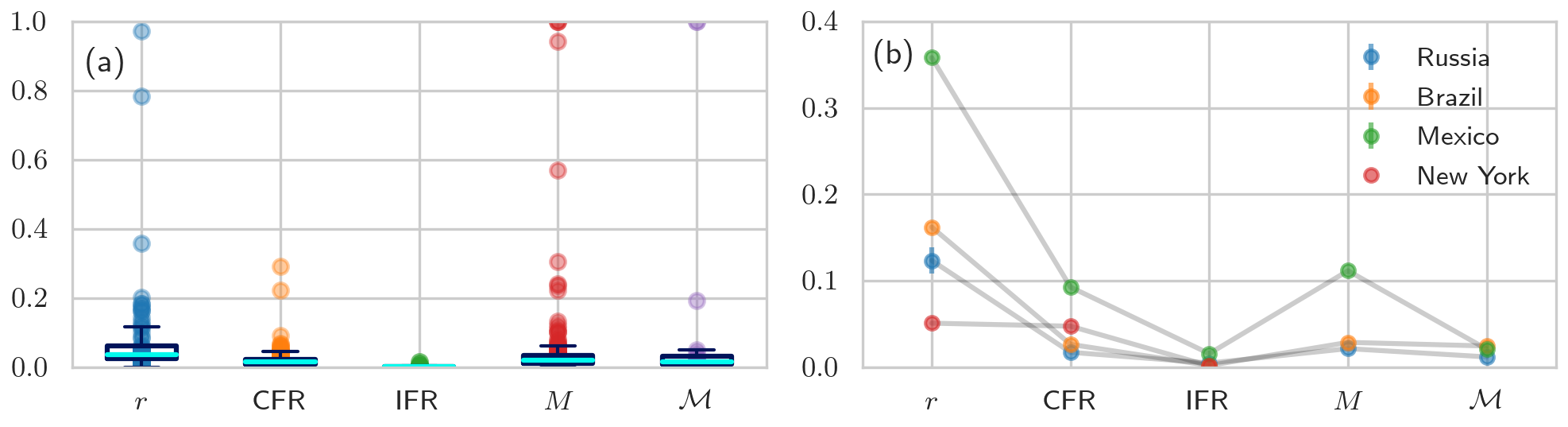
In Fig. 5(a), we show the values of the relative excess deaths $r$, the CFR, the apparent IFR, the confirmed resolved mortality $M$, and the true resolved mortality $\mathcal{M}$ for different (unlabeled) regions. In all cases we set $p=0.1,\gamma=100$. As illustrated in Fig. 5(b), some mortality measures suggest that COVID-induced fatalities are lower in certain countries compared to others, whereas other measures indicate the opposite. For example, the total resolved mortality $\mathcal{M}$ for Brazil is larger than for Russia and Mexico, most likely due to the relatively low number of reported excess deaths as can be seen from Fig. 3 (a). On the other hand, Brazil’s values of $\mathrm{CFR}$, $\mathrm{IFR}$, and $M$ are substantially smaller than those of Mexico [see Fig. 5(b)].

The distributions of all measures $Z$ and relative excess deaths $r$ across jurisdictions are shown Fig. 5(c–g) and encode the global uncertainty of these indices. We also calculate the corresponding mean values across jurisdictions, and use the empirical cumulative distribution functions to determine confidence intervals. The mean values across all jurisdictions are $\hbox{\vbox{\hrule height=0.5pt\kern 2.15277pt\hbox{\kern-1.00006pt$r$\kern-1.00006pt}}}=0.08$ (95% CI 0.0025–0.7800), $\hbox{\vbox{\hrule height=0.5pt\kern 2.15277pt\hbox{\kern-1.00006pt$\mathrm{CFR}$\kern-1.00006pt}}}=0.020$ (95% CI 0.0000–0.0565), $\hbox{\vbox{\hrule height=0.5pt\kern 2.15277pt\hbox{\kern-1.00006pt$\mathrm{IFR}$\kern-1.00006pt}}}=0.0024$ (95% CI 0.0000–0.0150), $\hbox{\vbox{\hrule height=0.5pt\kern 2.15277pt\hbox{\kern-1.00006pt$M$\kern-1.00006pt}}}=0.038$ (95% CI 0.0000–0.236), and $\hbox{\vbox{\hrule height=0.5pt\kern 2.15277pt\hbox{\kern-1.00006pt$\mathcal{M}$\kern-1.00006pt}}}=0.027$ (95% CI 0.000–0.193). For calculating   $M$ and   $\mathcal{M}$ , we excluded countries with incomplete recovery data. The distributions plotted in Fig. 5(c–g) can be used to inform our analyses of uncertainty or heterogeneity as summarized in Tab. 2. For example, the overall variance $\Sigma_{Z}^{2}$ can be determined by fitting the corresponding empirical $Z$ distribution shown in Fig. 5(c–g). Table 2 displays how the related $\rm{CV}_{Z}^{2}$ can be decomposed into separate terms, each arising from the variances associated to the components in the definition of $Z$. For concreteness, from Fig. 5(e) we obtain $\rm{CV}^{2}_{\rm IFR}={\Sigma_{\rm IFR}^{2}/\hbox{\vbox{\hrule height=0.5pt\kern 2.15277pt\hbox{\kern-1.00006pt$\mathrm{IFR}$\kern-1.00006pt}}}}^{2}\approx 1.16$ which allows us to place an upper bound on $\sigma_{b}^{2}$ using Eq. (A6), the results of Tab. 2, and

or on $\sigma_{\rm I}^{2}$ using $(1-\hat{f})^{2}\sigma_{\rm I}^{2}<(\tilde{f}_{\rm b}-{\rm FPR})^{2}{\rm CV}^{2}_{\rm IFR}$.

Finally, to provide more insight into the correlations between different mortality measures, we plot $M$ against $\mathrm{CFR}$ and $\mathcal{M}$ against $\mathrm{IFR}$ in Fig. 6. For most regions, we observe similar values of $M$ and $\mathrm{CFR}$ in Fig. 6(a). Althouigh we expect $M\to\mathrm{CFR}$ and $\mathcal{M}\to\mathrm{IFR}$ towards the end of an epidemic, in some regions such as the UK, Sweden, Netherlands, and Serbia, $M\gg{\rm CFR}$ due to unreported or incomplete reporting of recovered cases. About 50% of the regions that we show in Fig. 6(b) have an $\mathrm{IFR}$ that is approximately equal to $\mathcal{M}$. Again, for regions such as Sweden and the Netherlands, $\mathcal{M}$ is substantially larger than $\mathrm{IFR}$ because of incomplete reporting of recovered cases.

In the first few weeks of the initial COVID-19 outbreak in March and April 2020 in the US, the reported death numbers captured only about two thirds of the total excess deaths Woolf et al. 2020. This mismatch may have arisen from reporting delays, attribution of COVID-19 related deaths to other respiratory illnesses, and secondary pandemic mortality resulting from delays in necessary treatment and reduced access to health care Woolf et al. 2020. We also observe that the number of excess deaths in the Fall months of 2020 have been significantly higher than the corresponding reported COVID-19 deaths in many US states and countries. The weekly numbers of deaths in regions with a high COVID-19 prevalence were up to 8 times higher than in previous years. Among the countries that were analyzed in this study, the five countries with the largest numbers of excess deaths since the beginning of the COVID-19 outbreak (all numbers per 100,000) are Peru (256), Ecuador (199), Mexico (151), Spain (136), and Belgium (120). The five countries with the lowest numbers of excess deaths since the beginning of the COVID-19 outbreak are Denmark (2), Norway (6), Germany (8), Austria (31), and Switzerland (33) Exc 2020a ²² 2 Note that Switzerland experienced a rapid growth in excess deaths in recent weeks. More recent estimates of the number of excess deaths per 100,000 suggest a value of 64 Epidemic Datathon 2020, which is similar to the corresponding excess death value observed in Sweden.. If one includes the months before the outbreak, the numbers of excess deaths per 100,000 in 2020 in Germany, Denmark, and Norway are -3209, -707, and -34, respectively. In the early stages of the COVID-19 pandemic, testing capabilities were often insufficient to resolve rapidly-increasing case and death numbers. This is still the case in some parts of the world, in particular in many developing countries Ondoa et al. 2020. Standard mortality measures such as the IFR and CFR thus suffer from a time-lag problem.

The proposed use of excess deaths in standard mortality measures may provide more accurate estimates of infection-caused deaths, while errors in the estimates of the fraction of infected individuals in a population from testing can be corrected by estimating the testing bias and testing specificity and sensitivity. One could sharpen estimates of the true COVID-19 deaths by systematically analyzing the statistics of deaths from all reported causes using a standard protocol such as ICD-10 CDC 2020c. For example, the mean traffic deaths per month in Spain between 2011-2016 is about 174 persons EUROSTAT 2020, so any pandemic-related changes to traffic volumes would have little impact considering the much larger number of COVID-19 deaths.

Different mortality measures are sensitive to different sources of uncertainty. Under the assumption that all excess deaths are caused by a given infectious disease (e.g., COVID-19), the underlying error in the determined number of excess deaths can be estimated using historical death statistics from the same jurisdiction. Uncertainties in mortality measures can also be decomposed into the uncertainties of their component quantities, including the positive-tested fraction $f$ that depend on uncertainties in the testing parameters.

As for all epidemic forecasting and surveillance, our methodology depends on the quality of excess death and COVID-19 case data and knowledge of testing parameters. For many countries, the lack of binding international reporting guidelines, testing limitations, and possible data tampering Winter 2020 complicates the application of our framework. A striking example of variability is the large discrepancy between excess deaths $D_{\rm e}$ and confirmed deaths $D_{\rm c}$ across many jurisdictions which render mortalities that rely on $D_{\rm c}$ suspect. More research is necessary to disentangle the excess deaths that are directly caused by SARS-CoV-2 infections from those that result from postponed medical treatment Woolf et al. 2020, increased suicide rates Sher 2020, and other indirect factors contributing to an increase in excess mortality. Even if the numbers of excess deaths were accurately reported and known to be caused by a given disease, inferring the corresponding number of unreported cases (e.g., asymptomatic infections), which appears in the definition of the IFR and $\mathcal{M}$ (see Tab. 1), is challenging and only possible if additional models and assumptions are introduced.

Another complication may arise if the number of excess deaths is not significantly larger than the historical mean. Then, excess-death-based mortality estimates suffer from large uncertainty/variability and may be meaningless. While we have considered only the average or last values of $\tilde{f}_{\rm b}$, our framework can be straightforwardly extended and dynamically applied across successive time windows, using e.g., Bayesian or Kalman filtering approaches.

Finally, we have not resolved the excess deaths or mortalities with respect to age or other attributes such as sex, co-morbidities, occupation, etc. We expect that age-structured excess deaths better resolve a jurisdiction’s overall mortality. By expanding our testing and modeling approaches on stratified data, one can also straightforwardly infer stratified mortality measures $Z$, providing additional informative indices for comparison.

We tally weekly deaths according to Eq. (1) for each week $i$ starting from the first week of 2020, and cumulative excess deaths as in Eq. (2) adding all weekly contributions from the first week of 2020 onwards. Note that some governmental agencies tabulate weekly deaths starting on the Sunday closest to January 1 2020 (December 29 2019, such as the United States), others instead use January 1 2020 as the first day of the week (such as Germany). A detailed list of how each country bins weekly deaths is included in Ref. Exc 2020a. The final week $k$ up to which the cumulative count is taken depends on data availability, since some countries have larger reporting delays than others. In the majority of cases $k$ is beyond the fourth week of November 2020. Quantities are calculated from data that include deaths from typically $J=5$ previous years Exc 2020a.

In Fig. A2 we plot the weekly confirmed deaths $d_{\rm c}^{(0)}(i)$, the cumulative deaths $D_{\rm c}(k)=\sum_{i=1}^{k}d^{(0)}_{\rm c}(i)$, and the mean weekly and cumulative excess deaths $\bar{d}_{\rm e}(i)$ for 2020 as available from data. We also show $\bar{D}_{\rm e}(k)$ per 100,000 persons from the start of 2020 using Eqs. (1) and (2). The corresponding error bars in Fig. A2 indicate 95% confidence intervals defined by $\bar{d}_{\rm e}(i)\pm 1.96\,\sigma_{\rm e}(i)$ and $\bar{D}_{\rm e}(k)\pm 1.96\,\Sigma_{\rm e}(k)$ in Eqs. (1) and (2), respectively. For Spain, we used the 99% confidence intervals that are directly provided in the corresponding data Epidemic Datathon 2020 to approximate the 95% confidence intervals. Excess death statistics evolve differently across different countries and regions. For example, in France excess deaths were negative until the end of March 2020, quickly increasing in April 2020. In Ecuador and Peru, the number of excess deaths is more than 2.5 times larger than the corresponding number of confirmed COVID-19 deaths.

Given biases in sampling and testing errors, it is important to use a statistical testing model that takes them into account when estimating the fraction $f$ of a population $N$ that are infected. Testing biases arises, for example, if symptomatic individuals are more likely to seek testing. Thus, the probability $f_{\rm b}$ that an individual who chooses to be tested is positive may be different from $f$ the probability that a randomly selected individual is positive, as defined in Eq. (3). If all tests are error-free, the probability that $Q^{+}$ positive results arise from the $Q\geq Q^{+}$ administered tests is given by

Eq. (A1) is derived under the assumption that once individuals are tested, they are “replaced” in the population and can be tested again. The analogous distribution $P_{\rm true}(Q^{+}|Q,f_{\rm b})$ for testing “without replacement” can be straightforwardly derived and yields results quantitatively close to Eq. (A1) provided $Q/N\lesssim 0.3$.

Eq. (A1) also assumes flawless testing. Tests with Type I (false positives) and Type II (false negatives) may wrongly catalog uninfected individuals as infected (with rate FPR) while missing some infected individuals (with rate FNR). For serological COVID-19 tests, such as antibody tests, the estimated percentages of false positives and false negatives are typically low, with $\mathrm{FPR}\approx 0.03-0.07$ and $\mathrm{FNR}\approx 0.1$ U.S. Food and Drug Administration 2020, Cohen et al. 2020, Watson et al. 2020. For RT-PCR tests, the FNRs depend strongly on the actual assay method Lassauniere et al. 2020, Whitman et al. 2020 and typically lie between 0.1 and 0.3 Fang et al. 2020, Wang et al. 2020 but might be as high as $\mathrm{FNR}\approx 0.68$ if throat swabs are used Wang et al. 2020, Watson et al. 2020. FNRs can also vary significantly depending on how long after initial infection the test is administered Bastos et al. 2020. A systematic review conducted worldwide found ${\rm FNR}\approx 0.54$ at initial testing Arevalo-Rodriguez et al. 2020, underlying the need for retesting. Reported percentages of false positives in RT-PCR tests are about $\mathrm{FPR}\approx 0.05$ Watson et al. 2020. A large meta-analysis of serological tests estimates $\mathrm{FPR}\approx 0.02$ and $\mathrm{FNR}\approx 0.02-0.16$ Bastos et al. 2020. These testing errors can lead to inaccurate estimates of disease prevalence; uncertainty in FPR, FNR will thus lead to uncertainty in the estimate of prevalence.

As illustrated through Fig. 2, errors in testing may result in the recorded number $\tilde{Q}^{+}$ of positive tests to be different from the $Q^{+}$ that would be obtained under perfect testing. The probability that $\tilde{Q}^{+}$ positive tests are returned due to testing errors can be described in terms of $Q^{+}$, ${\rm FPR}$, and ${\rm FNR}$ and the corresponding probability distribution $P_{\rm err}(\tilde{Q}^{+}|Q^{+},\rm{FPR},\rm{FNR})$ is given by

where $q_{+}\equiv\tilde{Q}^{+}-p_{+}$. By convolving $P_{\rm err}(\tilde{Q}^{+}|Q^{+},\rm{FPR},\rm{FNR})$ with $P_{\rm true}(Q^{+}|Q,f_{\rm b})$ we derive the overall likelihood distribution for the measured number $\tilde{Q}^{+}$ of true and false positives given a set of specified parameters $\theta=\{Q,f,b,{\rm FPR},{\rm FNR}\}$ describing the population and testing

When $Q^{+},\tilde{Q}^{+}$, and $Q\gg 1$, we can approximate $P_{\rm true}$, $P_{\rm err}$, and $P$ by normal distributions and rewrite $P$ as a function of the observed positive fraction $\tilde{f}_{\rm b}\equiv\tilde{Q}^{+}/Q$ (Eqs. (4) and (5)).

Using Bayes’ rule, we can then formally define the likelihood of $\theta$ given a measured $\tilde{f}_{\rm b}$,

where $\alpha=\{\bar{\theta},\sigma_{\theta}\}$ are hyperparameters defining the prior $P_{0}(\theta|\alpha)$, such as their means $\bar{\theta}=\{\bar{D}_{\rm e},\hbox{\vbox{\hrule height=0.5pt\kern 2.15277pt\hbox{\kern-1.00006pt${\rm FPR}$\kern-1.00006pt}}},\hbox{\vbox{\hrule height=0.5pt\kern 2.15277pt\hbox{\kern-1.00006pt${\rm FNR}$\kern-1.00006pt}}},\bar{b},\bar{N}\}$ and standard deviations $\sigma_{\theta}=\{\Sigma_{\rm e},\sigma_{\rm I},\sigma_{\rm II},b,\sigma_{b},\sigma_{N}\}$. Formally, the probability of measuring a value of a mortality measure $Z={\rm CFR},{\rm IFR},M,{\cal M}$, or $r$, can be computed from

where $P(Z|\theta)$ defines the statistical model of the mortality measure given the components and parameters $\theta$ and the hyperparameters $\alpha$ defining the distribution over $\theta$. For example, if $Z$ is the value of the IFR, $\theta=\{D_{\rm e},f,N\}$ and $\alpha=\{(\bar{D}_{\rm e},\Sigma_{\rm e}),(\bar{b},\hbox{\vbox{\hrule height=0.5pt\kern 2.15277pt\hbox{\kern-1.00006pt${\rm FPR}$\kern-1.00006pt}}},\hbox{\vbox{\hrule height=0.5pt\kern 2.15277pt\hbox{\kern-1.00006pt${\rm FNR}$\kern-1.00006pt}}},\sigma_{b},\sigma_{\rm I},\sigma_{\rm II}),(\bar{N},\Sigma_{N})\}$ are the mean and standard deviation of excess deaths, testing parameters, and the total population, respectively.

A simpler way to incorporate uncertainty in the infected fraction $f$ is to assume a Gaussian approximation for all distributions and propagate the uncertainty in testing parameters. The squared coefficient of variation ${\rm CV}_{f}^{2}$ is then decomposed into the parameter variances according to

where $X\equiv\tilde{f}_{\rm b}-{\rm FPR}$. The values of $b$, ${\rm FPR}$, ${\rm FNR}$ above are mean or maximum likelihood estimates of the bias and testing errors, and $\sigma_{b}^{2}$, $\sigma_{\rm I}^{2}$, and $\sigma_{\rm II}^{2}$ are their associated uncertainties. The means and variances $\{\bar{b},\hbox{\vbox{\hrule height=0.5pt\kern 2.15277pt\hbox{\kern-1.00006pt${\rm FPR}$\kern-1.00006pt}}},\hbox{\vbox{\hrule height=0.5pt\kern 2.15277pt\hbox{\kern-1.00006pt${\rm FNR}$\kern-1.00006pt}}},\sigma_{b}^{2},\sigma_{\rm I}^{2},\sigma_{\rm II}^{2}\}$ represent hyperparameters associated with testing (see SI). Our result for $\sigma_{f}^{2}$ in Eq. (A6) assumes $\{b,{\rm FPR},{\rm FNR}\}$ are uncorrelated. Since $Q\gg 1$ is typically large, we expect the first contribution to the uncertainty, arising from stochasticity in the sampling and proportional to $\tilde{f}_{\rm b}(1-\tilde{f}_{\rm b})/Q$ to be negligible. Uncertainties in other quantities will ultimately contribute to uncertainty in the mortalities $Z$, as listed in Table 2.

In Fig. A3, we show the evolution of $\mathcal{M}$ for Spain and Lombardia, using different effective recovery rates of unreported cases $\gamma$. We compute $\mathcal{M}$ according to Eq. (8) and use excess mortality data of Fig. A1 to determine $\bar{D}_{\rm e}$. The corresponding data for confirmed recovered and deceased individuals, $R_{\rm c}$ and $D_{\rm c}$, is taken from Ref. Epidemic Datathon 2020. Current estimates of the IFR are $0.1-1.5$% Salje et al. 2020, Chow et al. 2020, Ioannidis 2020. To obtain a value of $\mathcal{M}$ in a similar range, we vary $\gamma$ from $1-1000$ and find that $\mathcal{M}\approx 0.1-1$% is consistent with $\gamma=100-1000$.

References

- World Health Organization (2020a) World Health Organization. WHO Director-General’s opening remarks at the media briefing on COVID-19 - 11 March 2020. https://www.who.int/dg/speeches/detail/who-director-general-s-opening-remarks-at-the-media-briefing-on-covid-19---11-march-2020, 2020a. Accessed: 2020-04-18.
- cor (2020) COVID-19 statistics. https://www.worldometers.info/coronavirus/, 2020. Accessed: 2021-01-05.
- He et al. (2020) Xi He, Eric HY Lau, Peng Wu, Xilong Deng, Jian Wang, Xinxin Hao, Yiu Chung Lau, Jessica Y Wong, Yujuan Guan, Xinghua Tan, et al. Temporal dynamics in viral shedding and transmissibility of COVID-19. Nature Medicine, 26(5):672–675, 2020.
- CDC (2020a) Conditions contributing to deaths involving coronavirus disease 2019 (COVID-19), by age group and state, United States. https://data.cdc.gov/NCHS/Conditions-contributing-to-deaths-involving-corona/hk9y-quqm, 2020a. Accessed: 2020-09-26.
- Morris and Reuben (2020) Chris Morris and Anthony Reuben. Coronavirus: Why are international comparisons difficult?, BBC Reality Check. https://www.bbc.com/news/52311014, 2020. Accessed: 2020-09-13.
- Beaney et al. (2020) Thomas Beaney, Jonathan M Clarke, Vageesh Jain, Amelia Kataria Golestaneh, Gemma Lyons, David Salman, and Azeem Majeed. Excess mortality: the gold standard in measuring the impact of COVID-19 worldwide? Journal of the Royal Society of Medicine, 113(9):329–334, 2020.
- Onder et al. (2020) Graziano Onder, Giovanni Rezza, and Silvio Brusaferro. Case-fatality rate and characteristics of patients dying in relation to COVID-19 in Italy. JAMA, 2020.
- CDC (2020b) CDC. Understanding the Numbers: Provisional Death Counts and COVID-19. https://www.cdc.gov/nchs/data/nvss/coronavirus/Understanding-COVID-19-Provisional-Death-Counts.pdf, 2020b. Accessed: 2020-10-06.
- Keeling and Rohani (2011) Matt J Keeling and Pejman Rohani. Modeling infectious diseases in humans and animals. Princeton University Press, 2011.
- Böttcher et al. (2020) Lucas Böttcher, Mingtao Xia, and Tom Chou. Why case fatality ratios can be misleading: individual-and population-based mortality estimates and factors influencing them. Physical Biology, 17:065003, 2020.
- Böttcher et al. (2017) Lucas Böttcher, Jan Nagler, and Hans J Herrmann. Critical behaviors in contagion dynamics. Physical Review Letters, 118(8):088301, 2017.
- Böttcher and Antulov-Fantulin (2020) Lucas Böttcher and Nino Antulov-Fantulin. Unifying continuous, discrete, and hybrid susceptible-infected-recovered processes on networks. Physical Review Research, 2(3):033121, 2020.
- Pastor-Satorras et al. (2015) Romualdo Pastor-Satorras, Claudio Castellano, Piet Van Mieghem, and Alessandro Vespignani. Epidemic processes in complex networks. Reviews of Modern Physics, 87(3):925, 2015.
- Faust et al. (2020) Jeremy Samuel Faust, Zhenqiu Lin, and Carlos Del Rio. Comparison of estimated excess deaths in new york city during the COVID-19 and 1918 influenza pandemics. JAMA Network Open, 3(8):e2017527–e2017527, 2020.
- Woolf et al. (2020) Steven H Woolf, Derek A Chapman, Roy T Sabo, Daniel M Weinberger, and Latoya Hill. Excess deaths from COVID-19 and other causes, March-April 2020. Jama, 324(5):510–513, 2020.
- Kontis et al. (2020) Vasilis Kontis, James E Bennett, Theo Rashid, Robbie M Parks, Jonathan Pearson-Stuttard, Michel Guillot, Perviz Asaria, Bin Zhou, Marco Battaglini, Gianni Corsetti, et al. Magnitude, demographics and dynamics of the effect of the first wave of the COVID-19 pandemic on all-cause mortality in 21 industrialized countries. Nature Medicine, pages 1–10, 2020.
- Git (2020) GitHub repository. https://github.com/lubo93/disease-testing, 2020.
- World Health Organization (2020b) World Health Organization. Estimating mortality from COVID-19. Department of Communications, Global Infectious Hazard Preparedness, WHO Global, 2020b.
- Xu et al. (2020) Zhe Xu, Lei Shi, Yijin Wang, Jiyuan Zhang, Lei Huang, Chao Zhang, Shuhong Liu, Peng Zhao, Hongxia Liu, Li Zhu, et al. Pathological findings of COVID-19 associated with acute respiratory distress syndrome. Lancet Resp. Med., 2020.
- Dong et al. (2020) Ensheng Dong, Hongru Du, and Lauren Gardner. An interactive web-based dashboard to track COVID-19 in real time. The Lancet Infectious Diseases, 2020.
- CDC (2020) CDC. Pneumonia and Influenza Mortality Surveillance from the National Center for Health Statistics Mortality Surveillance System. https://gis.cdc.gov/grasp/fluview/mortality.html, 2020. Accessed: 2020-12-10.
- MoMo Spain (2020) MoMo Spain. MoMo Spain. https://momo.isciii.es/public/momo/dashboard/momo_dashboard.html#datos, 2020. Accessed: 2020-12-10.
- Office for National Statistics (2020) Office for National Statistics. Deaths registered weekly in England and Wales, provisional. https://www.ons.gov.uk/peoplepopulationandcommunity/birthsdeathsandmarriages/deaths/datasets/weeklyprovisionalfiguresondeathsregisteredinenglandandwales, 2020. Accessed: 2020-12-10.
- Bundesamt für Statistik (2020) Bundesamt für Statistik. Sterblichkeit, Todesursachen. https://www.bfs.admin.ch/bfs/de/home/statistiken/gesundheit/gesundheitszustand/sterblichkeit-todesursachen.html, 2020. Accessed: 2020-07-16.
- Istituto Nazionale di Statistica (2020) Istituto Nazionale di Statistica. Dati di mortalità: cosa produce l’Istat. https://www.istat.it/it/archivio/240401, 2020. Accessed: 2020-07-08.
- Epidemic Datathon (2020) Epidemic Datathon. Summary of historical and current mortality data. https://www.epidemicdatathon.com/data, 2020. Accessed: 2020-12-10.
- Exc (2020a) The Economist’s tracker for COVID-19 excess deaths. https://github.com/TheEconomist/covid-19-excess-deaths-tracker, 2020a. Accessed: 2020-12-10.
- EURO MOMO (2020) EURO MOMO. Mortality monitoring in Europe. https://www.euromomo.eu/index.html, 2020. Accessed: 2020-12-10.
- Exc (2020b) Excess Deaths Associated with COVID-19. https://www.cdc.gov/nchs/nvss/vsrr/covid19/excess_deaths.htm, 2020b. Accessed: 2020-12-10.
- Li et al. (2020) Ruiyun Li, Sen Pei, Bin Chen, Yimeng Song, Tao Zhang, Wan Yang, and Jeffrey Shaman. Substantial undocumented infection facilitates the rapid dissemination of novel coronavirus (SARS-CoV2). Science, 2020. ISSN 0036-8075.
- Chow et al. (2020) Carson C Chow, Joshua C Chang, Richard C Gerkin, and Shashaank Vattikuti. Global prediction of unreported sars-cov2 infection from observed covid-19 cases. medRxiv, 2020.
- Salje et al. (2020) Henrik Salje, Cécile Tran Kiem, Noémie Lefrancq, Noémie Courtejoie, Paolo Bosetti, Juliette Paireau, Alessio Andronico, Nathanaël Hozé, Jehanne Richet, Claire-Lise Dubost, et al. Estimating the burden of SARS-CoV-2 in France. Science, 2020.
- Ioannidis (2020) John Ioannidis. The infection fatality rate of COVID-19 inferred from seroprevalence data. medRxiv, 2020.
- NYC Health (2020) NYC Health. COVID-19: Data. https://www1.nyc.gov/site/doh/covid/covid-19-data.page, 2020. Accessed: 2020-12-10.
- Liu (2020) Yi Liu. COVID-19 Coronavirus Map repository. https://github.com/stevenliuyi/covid19, 2020. Accessed: 2020-04-20.
- Times (2020) New York Times. Coronavirus (Covid-19) Data in the United States. https://github.com/nytimes/covid-19-data, 2020. Accessed: 2020-12-10.
- Lee and Forthofer (2006) Eun Sul Lee and Ronald N Forthofer. Analyzing complex survey data. SAGE, 2006.
- CDC (2020a) CDC. Guidance for Certifying Deaths Due to Coronavirus Disease 2019 (COVID–19). https://www.cdc.gov/nchs/data/nvss/vsrg/vsrg03-508.pdf, 2020a. Accessed: 2020-11-20.
- Watson et al. (2020) Jessica Watson, Penny F Whiting, and John E Brush. Interpreting a COVID-19 test result. BMJ, 369, 2020.
- Fang et al. (2020) Yicheng Fang, Huangqi Zhang, Jicheng Xie, Minjie Lin, Lingjun Ying, Peipei Pang, and Wenbin Ji. Sensitivity of chest CT for COVID-19: comparison to RT-PCR. Radiology, page 200432, 2020.
- Wang et al. (2020) Wenling Wang, Yanli Xu, Ruqin Gao, Roujian Lu, Kai Han, Guizhen Wu, and Wenjie Tan. Detection of SARS-CoV-2 in different types of clinical specimens. JAMA, 323(18):1843–1844, 2020.
- CDC (2020b) COVIDView. https://www.cdc.gov/coronavirus/2019-ncov/covid-data/covidview/index.html, 2020b. Accessed: 2020-12-10.
- Cen (2020) Census Bureau Estimates U.S. Population Reached 330 Million Today. https://data.cdc.gov/NCHS/Conditions-contributing-to-deaths-involving-corona/hk9y-quqm, 2020. Accessed: 2020-09-26.
- Hortaccsu et al. (2020) Ali Hortaccsu, Jiarui Liu, and Timothy Schwieg. Estimating the fraction of unreported infections in epidemics with a known epicenter: an application to COVID-19. Technical report, National Bureau of Economic Research, 2020.
- Ondoa et al. (2020) Pascale Ondoa, Yenew Kebede, Marguerite Massinga Loembe, Jinal N Bhiman, Sofonias Kifle Tessema, Abdourahmane Sow, John Nkengasong, et al. COVID-19 testing in Africa: lessons learnt. The Lancet Microbe, 1(3):e103–e104, 2020.
- CDC (2020c) CDC. International Classification of Diseases,Tenth Revision (ICD-10). https://www.cdc.gov/nchs/icd/icd10.htm, 2020c. Accessed: 2020-04-19.
- EUROSTAT (2020) EUROSTAT. Death due to transport accidents, by sex. https://ec.europa.eu/eurostat/databrowser/view/tps00165/default/table?lang=en, 2020. Accessed: 2020-04-20.
- Winter (2020) Laura Winter. Data fog: Why some countries’ coronavirus numbers do not add up. https://www.aljazeera.com/indepth/features/data-fog-countries-coronavirus-numbers-add-200607065953544.html, 2020. Accessed: 2020-09-14.
- Sher (2020) Leo Sher. The impact of the COVID-19 pandemic on suicide rates. QJM: An International Journal of Medicine, 113(10):707–712, 2020.
- U.S. Food and Drug Administration (2020) U.S. Food and Drug Administration. EUA authorized serology test performance. https://www.fda.gov/medical-devices/emergency-situations-medical-devices/eua-authorized-serology-test-performance, 2020.
- Cohen et al. (2020) Andrew N Cohen, Bruce Kessel, and Michael G Milgroom. Diagnosing COVID-19 infection: the danger of over-reliance on positive test results. medRxiv, 2020.
- Lassauniere et al. (2020) Ria Lassauniere, Anders Frische, Zitta B Harboe, Alex CY Nielsen, Anders Fomsgaard, Karen A Krogfelt, and Charlotte S Jorgensen. Evaluation of nine commercial SARS-CoV-2 immunoassays. medRxiv, 2020.
- Whitman et al. (2020) Jeffrey D Whitman, Joseph Hiatt, Cody T Mowery, Brian R Shy, Ruby Yu, Tori N Yamamoto, Ujjwal Rathore, Gregory M Goldgof, Caroline Whitty, Jonathan M Woo, et al. Test performance evaluation of SARS-CoV-2 serological assays. medRxiv, 2020.
- Bastos et al. (2020) Mayara Lisboa Bastos, Gamuchirai Tavaziva, Syed Kunal Abidi, Jonathon R Campbell, Louis-Patrick Haraoui, James C Johnston, Zhiyi Lan, Stephanie Law, Emily MacLean, Anete Trajman, et al. Diagnostic accuracy of serological tests for COVID-19: systematic review and meta-analysis. BMJ, 370, 2020.
- Arevalo-Rodriguez et al. (2020) Ingrid Arevalo-Rodriguez, Diana Buitrago-Garcia, Daniel Simancas-Racines, Paula Zambrano-Achig, Rosa del Campo, Agustin Ciapponi, Omar Sued, Laura Martinez-Garcia, Anne Rutjes, Nicola Low, et al. False-negative results of initial RT-PCR assays for COVID-19: a systematic review. medRxiv, 2020.
Supplementary Information
Examples of excess death data