Elastic 3D-2D Image Registration

In this article we propose an elastic 3D-2D image registration technique, which is motivated by a challenging image processing problem arising in biological studies of leucocyte extravasation into inflamed tissue in mice. A common experimental procedure consists of irritating a certain tissue region and performing two-dimensional intravital microscopy (IVM) to monitor the reactions on the cellular level, see for instance [4]. After a sufficiently long video sequence has been recorded, the animal is sacrificed, the tissue is removed, stained, and fixed, and a single, volumetric 3D image is acquired using a 3D confocal microscope. The two obtained datasets therefore show essentially the same tissue region, one being an elastically deformed configuration of the other. While the IVM recording shows in addition the temporal behaviour of the moving leucocytes, the confocal microscopy image contains more detailed structures such as the blood vessel basement membranes. Aligning and merging both datasets allows to combine the enhanced structural information obtained by the 3D confocal microscope with temporal information gained from the IVM.

Both the 2D and 3D dataset use flourescent staining and thus possess multiple colour channels corresponding to different flourescent dyes. In particular, one channel of both images contains the same biological structures (for instance the endothelial cell membranes) so that those can be used for registration. Our approach for registering the images is based on mimicking the image acquisition system of the 2D microscope, including a non-rigid tissue deformation and a blurring and projection step. The intensities of the blurred and projected image volume are then compared with those of a 2D reference image (for instance a single frame of the IVM video), see fig. 1 for the overall procedure. The goal of the registration process is then to find a deformation transforming the volumetric image in such a way that the similarity of the two datasets is maximal. The set of admissible deformations is chosen in a way that reflects physical properties of the underlying tissue.

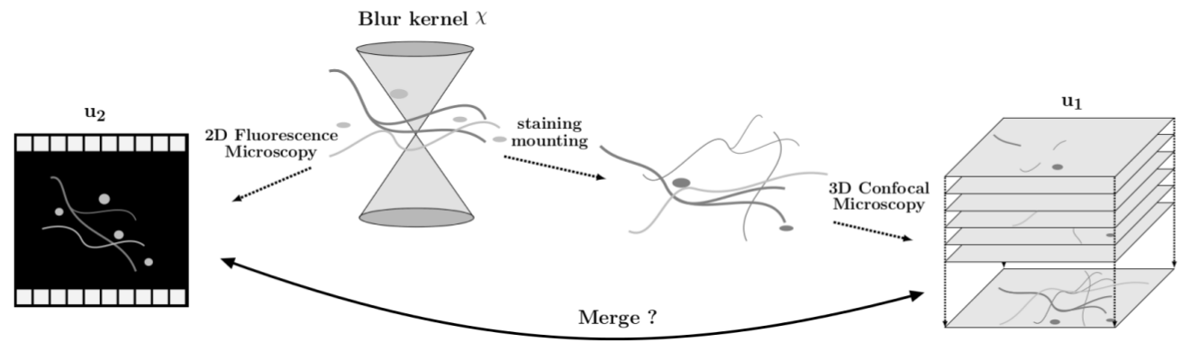
In this article, we present a complete mathematical description of the aforementioned procedure and, using the direct method in the calculus of variations, guarantee the existence of an admissible deformation which maximizes the similarity between the datasets. Although rigid or parameterized 3D-2D registration [18, 25] and elastic 3D-3D registration [3] has been studied before, elastic 3D-2D registration has so far not been attempted to the best of our knowledge.

Xu and Wan presented an intensity based 3D-2D registration technique for the matching of a CT volume to 2D X-Ray images and a description of how their method can be implemented on GPUs [24]. Studies on CT to X-Ray Fluoroscopy registration for guidance of surgical intervention were published by Otake et al. [18] and Uneri et al. [23]. All three articles employ rigid motions to obtain optimal alignment, which can be expected to yield satisfactory registration results for this specific type of problem.

Also descriptions of nonrigid methods can be found in the literature. Zheng and Yu presented a spline based 3D-2D registration technique [25] for matching 3D CT data to 2D X-Ray images using a statistical deformation model. The article also references a number of publications which describe similar methods. In contrast to our setting, in all above studies the 2D images result from a 3D volume via the X-Ray transform, while our 2D images stem from optical microscopy and thus depict structures outside the focus plane with blur. On the one hand this blur makes the lateral alignment of structures between the 3D and 2D image more difficult (also computationally), on the other hand it can provide additional information about the deformation along the viewing direction, which in the above studies must come solely from the deformation model.

Heldmann and Papenberg presented a variational method to register 3D CT data to a sequence of 2D ultrasound slices [10]. Note that their 2D images thus stem from point- or slicewise evaluation of a 3D volume rather than from an integral transform as in our and the above approaches. The well-posedness of this problem thus requires high regularity of the 3D image to be registered and the corresponding deformation, which the authors provide employing curvature regularization. They include results of the application of their technique to clinical data, however, no in depth analysis of the presented energy functional is presented. Berkels et al. studied 2D-3D surface registration, where graph representations of cortical surfaces had to be matched to 2D brain images. Unlike in our case, an optimal deformation $\psi:\mathbb{R}^{2}\to\mathbb{R}^{3}$ had to be found. For the regularization of this highly ill-posed problem, the authors suggested a regularizer based on the second order thin plate spline energy of $\psi$ [2]. A different, yet still related, situation can arise in surface to surface matching problems, if surface regions are locally described by two dimensional images which then in turn can be processed further by 2D-2D image matching algorithms. Such methods were for example described by Merelli et al. [14, 15].

Our method will estimate displacement in viewing direction from the severity of out of focus blur. A closely related problem, known as depth-from-defocus, is to estimate the distance between an object and the image acquisition device from a whole image stack (rather than just one image as in our case) that was generated by capturing the object under varying focal settings. The forward model described by Persch et al. [20], which mimics the image acquisition of a thin lens camera, is comparable to our 2D microscope model. Likewise related is the article by Aguet et al. [1], which suggests a method of how an image stack, produced by moving a sample through the different focal planes of a 2D microscope, can be combined into a single feature enriched image.

For further methods we refer to the extensive overview [13] of 3D-2D registration techniques with a focus on applications in image guided surgery.

In the next section we present the mathematical model and the analysis of existence of solutions in detail. Section 3 describes the numerical implementation, while section 4 shows the behaviour of the method in carefully chosen test cases and a real biological dataset.

We continue with the mathematical description of our registration problem. We first briefly describe the forward operator of the 2D microscope and subsequently a physically reasonable model of tissue deformations.

For simplicity, our exposition will consider the 3D and 2D unit domains ${\Omega_{\text{3D}}}=[-1,1]^{3}$ and ${\Omega_{\text{2D}}}=[-1,1]^{2}$, respectively. The volumetric image stemming from 3D confocal microscopy is denoted $u_{\text{3D}}:{\Omega_{\text{3D}}}\to[0,\infty)$ and is considered to represent the tissue reference configuration. In comparison to the IVM the quality of the 3D microscopy process is typically good enough to assume $u_{\text{3D}}$ noise- and blurfree. The 2D microscopy image $u_{\text{2D}}:{\Omega_{\text{2D}}}\to[0,\infty)$ will be interpreted as resulting from a non-rigid deformation of $u_{\text{3D}}$ and a subsequent projection into the plane. Above, both $u_{\text{3D}}$ and $u_{\text{2D}}$ are assumed to represent only that colour channel in which the same biological structures are visible; furthermore we will assume both images to be uniformly bounded (which is appropriate since the image intensities can be interpreted as the local concentration of fluorescent molecules).

The forward operator of 2D microscopy can be modelled by

where the blurring kernel $\chi\in L^{1}(\mathbb{R}^{3})$ has compact support and encodes the microscope’s point spread function. Above, $L^{p}$ denotes the standard Lebesgue function space, and $\chi\ast u$ denotes convolution (after extending $u$ by zero outside ${\Omega_{\text{3D}}}$). Due to

we have $\chi\ast u\in C_{c}^{0}(\mathbb{R}^{3})$ (the space of continuous functions with compact support) so that ${\mathcal{F}}$ is well-defined and even maps into $C^{0}({\Omega_{\text{2D}}})$ (the space of continuous functions on ${\Omega_{\text{2D}}}$). The value $\chi((x_{1},x_{2},0)-z)$ can be interpreted as the amount of light recorded at $(x_{1},x_{2})$ by the 2D microscope from a point source of light at $z$, which is readily seen from $({\mathcal{F}}u)(x_{1},x_{2})=\int_{\mathbb{R}^{3}}\chi((x_{1},x_{2},0)-z)u(z)\,{\mathrm{d}}z$. In our model we assume the blurring kernel to be spatially independent so that the observed blur of a point $z\in{\Omega_{\text{3D}}}$ only depends on its height $z_{3}$. A simple example (used in our calculations due to lack of a properly measured point spread function) is given by

which blurs each point $z$ outside the focus plane $\mathbb{R}^{2}\times\{0\}$ uniformly onto a disc of radius $cz_{3}$.

Between the 2D and the 3D image acquisition the tissue is deformed by a deformation $y:{\Omega_{\text{3D}}}\to\mathbb{R}^{3}$, where for any point $x\in{\Omega_{\text{3D}}}$ the value $y(x)$ shall be interpreted as the new position assumed during the 3D image acquisition. The inverse deformation $y^{-1}$ thus moves the reference configuration back into the configuration during the 2D microscopy so that we expect $u_{\text{2D}}={\mathcal{F}}(u_{\text{3D}}\circ y)$. However, due to noise in the image acquisition and additional artefacts not included in our model (such as diffuse background signals) one cannot expect equality. Instead we shall seek a deformation $y$ that leads to a small dissimilarity measure

where $d:\mathbb{R}\times\mathbb{R}\to[0,\infty)$ measures the distance between two image intensities (again $u_{\text{3D}}$ is extended by zero outside ${\Omega_{\text{3D}}}$). The optimal choice of $d$ is in general determined by the type of noise contained in the image data. We will focus on the $L^{1}$ and $L^{2}$ distance measures obtained with

respectively. The former is well-known to be appropriate if the data contains strong outliers, while the latter is appropriate for additive Gaussian noise. Other choices include correlation-based distance measures (see for instance [16, Sct. 6.1]) or the Kullback–Leibler Divergence $d_{\text{KL}}(a,b)=b-a+a\log\frac{a}{b}$ in case of Poisson noise.

The minimization of $\mathcal{J}^{d}[y]$ for general mappings $y:{\Omega_{\text{3D}}}\to\mathbb{R}^{3}$ is neither physically reasonable nor well-posed. Indeed, $y$ might be discontinuous or not even measurable so that the composition $u_{\text{3D}}\circ y$ does not make sense. Thus we have to regularize the deformation $y$ by imposing additional constraints and adding an extra energy term. Concerning physical constraints, $y$ should neither reverse the orientation of the deformed body ${\Omega_{\text{3D}}}$ nor should it introduce self-intersections of the material. The first condition translates to

whereas the second condition is imposed by additionally demanding

where ${\mathrm{vol}}$ shall denote the three-dimensional Lebesgue measure. The advantage of this constraint is that it guarantees the injectivity of $y$ if combined with $\det\nabla y>0$ and that it also holds for the weak limit of a sequence $(y_{k})_{k}$ satisfying the constraint, see for example [5, Thm. 7.9-1]. We shall also constrain the maximal possible displacement according to

in order not to shift the three-dimensional volume out of the visible area. In addition to those hard constraints, unreasonable growth or shrinkage of lengths, areas, or volumes by the deformation should be penalized. Modelling the biological tissue as an elastic material, such a penalization can be achieved by adding an elastic deformation energy

as regularization, which will prevent physically unreasonable deformations with too high elastic energy. Here, $W:\mathbb{R}^{3\times 3}\to[0,\infty)$ represents the stored energy function. Since biological tissue is very soft, it typically undergoes considerable nonlinear deformation so that the elastic model should be geometrically nonlinear and, in particular, rigid motion invariant. Furthermore, due to lack of better information we may assume a homogeneous and isotropic elastic constitutive law. Together, the above assumptions imply that the stored energy function can be written as a function of the singular values or of the invariants of its argument (see for example [5, Ch. 4]) so that

with the Frobenius norm $\|A\|_{F}=\sqrt{\mathrm{tr}(A^{T}A)}$ and the cofactor matrix ${\mathrm{cof}}A=\det AA^{-T}$. Note that $\|A\|_{F}$, $\|{\mathrm{cof}}A\|_{F}$, and $\det A$ control length, area, and volume changes respectively. Furthermore, biological tissue is almost incompressible so that deviation from $\det\nabla y=1$ should be strongly penalized. In our numerical experiments we will use the particular example

for a positive constant $c_{1}$ and a function $g:\mathbb{R}\to[0,\infty)$ such that $g(x)\to\infty$ for $x\to 0$. To favour deformations obeying $\det\nabla y\approx 1$, a term like $|\det\nabla y-1|^{2}$ can be incorporated into the definition of $g$. Note that this function is polyconvex (that is, can be written as a convex function of $(\nabla y,{\mathrm{cof}}\nabla y,\det\nabla y)$), which ensures weak lower semi-continuity of ${\mathcal{R}}$ as will be needed for the existence analysis. Summarizing, we arrive at the optimization problem

whose solution is the sought matching deformation.

In this section we discuss the discretization and numerical minimization of the energy functional

which is nontrivial due to the nonlocal convolution operator in ${\mathcal{F}}$, the composition of discretized functions, and the nondifferentiability of the discretized functions. As before, $d$ denotes either the Euclidean distance $d_{1}(x,y)=|x-y|$ or its square $d_{2}(x,y)=|x-y|^{2}$, but other choices can be implemented in the same way. To obtain a differentiable functional in the former case (which will allow simpler numerics), we make the modification $d_{1}(x,y)=\sqrt{(x-y)^{2}+\delta^{2}}$ with $\delta>0$ a small regularization parameter. In our implementation the stored energy function $W$ has the form

with constants $c_{1},c_{2},c_{3}\geq 0$, $D\in\mathbb{R}$ such that $W\geq 0$ and $W(S)=0$ for rotation matrices $S$. This specific choice violates the growth condition of theorem 1 (which was needed to apply a change of variables formula for Sobolev functions, while the lower semi-continuity of ${\mathcal{R}}$ could also be obtained for weaker growth conditions [19, Thm. 3.6]), however, we observed no indication of degeneration of the deformations in our numerical experiments so that the above choice seemed sufficient. Note that other stored energy functions can be implemented just as well, for instance the strain energy densities of Neo-Hookean materials,

which only differ from our choice by the slightly weaker penalty term for volume compression. Note also that in our experiments the constraints $\int_{{\Omega_{\text{3D}}}}\det\,\nabla y(x)\,{\mathrm{d}}x\leq{\mathrm{vol}}(y({\Omega_{\text{3D}}}))$ and $\|y\|_{L^{\infty}}\leq{\mathrm{diam}}({\Omega_{\text{2D}}})$ were always satisfied without explicit enforcement.

Assuming a twice differentiable 3D image $u_{\text{3D}}$, the first and second Gâteaux derivatives of $\mathcal{J}^{d}$ in $y\in\mathcal{A}$ for suitable variations $\phi$ and $\psi$ are

where $\mathrm{Hess}\,u_{\text{3D}}$ denotes the Hessian of $u_{\text{3D}}$. While for convex $d$ the second summand in $\partial^{2}\mathcal{J}^{d}[y]$ is always positive semi-definite, the first summand may destroy this definiteness. For the sake of completeness, we also write down the expressions for the first and second Gâteaux derivative of the hyperelastic regularizer. Rewriting $W$ defined in (1) in the form

its partial derivatives are given by

With the help of the identities $\partial_{A}\det(A)(B)=\mathrm{tr}(B^{T}{\mathrm{cof}}A)$ and $\partial_{A}(\|A\|_{F}^{2})(B)=2\mathrm{tr}(B^{T}A)$ and abbreviating $I_{1}=\|\nabla y\|_{F}^{2}$ and $I_{3}=\det\nabla y$, the Gâteaux derivatives of the hyperelastic regularizer read

References

- [1] F. Aguet, D. Van De Ville, and M. Unser. Model-based 2.5-d deconvolution for extended depth of field in brightfield microscopy. IEEE Transactions on Image Processing, 17(7):1144–1153, July 2008.
- [2] Benjamin Berkels, Ivan Cabrilo, Sven Haller, Martin Rumpf, and Karl Schaller. Co-registration of intra-operative brain surface photographs and pre-operative mr images. International Journal of Computer Assisted Radiology and Surgery, 9(3):387–400, May 2014.
- [3] M. Burger, J. Modersitzki, and L. Ruthotto. A hyperelastic regularization energy for image registration. SIAM Journal on Scientific Computing, 35(1):B132–B148, 2013.
- [4] Konrad Buscher, Huiyu Wang, Xueli Zhang, Paul Striewski, Benedikt Wirth, Gurpanna Saggu, Stefan Lütke-Enking, Tanya N. Mayadas, Klaus Ley, Lydia Sorokin, and Jian Song. Protection from septic peritonitis by rapid neutrophil recruitment through omental high endothelial venules. Nature Communications, 7:10828, 2016.
- [5] P.G. Ciarlet. Three-Dimensional Elasticity. Mathematical Elasticity. Elsevier Science, 1988.
- [6] P.G. Ciarlet, A. Buttigieg, D.G. Crighton, A. Buttigieg, B. Miara, J.M. Thomas, M.J. Ablowitz, S.H. Davis, E.J. Hinch, A. Iserles, et al. Introduction to Numerical Linear Algebra and Optimisation. Cambridge Texts in Applied Mathematics. Cambridge University Press, 1989.
- [7] Gene H. Golub and Charles F. Van Loan. Matrix Computations (3rd Ed.). Johns Hopkins University Press, Baltimore, MD, USA, 1996.
- [8] Nicholas IM Gould, Stefano Lucidi, Massimo Roma, and Philippe L Toint. Solving the trust-region subproblem using the lanczos method. SIAM Journal on Optimization, 9(2):504–525, 1999.
- [9] Ghassan Hamarneh and Preet Jassi. Vascusynth: Simulating vascular trees for generating volumetric image data with ground-truth segmentation and tree analysis. Comp. Med. Imag. and Graph., 34(8):605–616, 2010.
- [10] Stefan Heldmann and Nils Papenberg. A variational approach for volume-to-slice registration. In Scale Space and Variational Methods in Computer Vision, pages 624–635, Berlin, Heidelberg, 2009. Springer Berlin Heidelberg.
- [11] Sébastien Loriot, Olga Sorkine-Hornung, Yin Xu, and Ilker O. Yaz. Triangulated surface mesh deformation. In CGAL User and Reference Manual. CGAL Editorial Board, 5.1.1 edition, 2020.
- [12] M. Marcus and V. J. Mizel. Transformations by functions in Sobolev spaces and lower semicontinuity for parametric variational problems. Bull. Amer. Math. Soc., 79(4):790–795, 07 1973.
- [13] P. Markelj, D. Tomaževič, B. Likar, and F. Pernuš. A review of 3d/2d registration methods for image-guided interventions. Medical Image Analysis, 16(3):642 – 661, 2012. Computer Assisted Interventions.
- [14] I. Merelli, P. Cozzi, D. D’Agostino, A. Cleamatis, and L. Milanesi. Images based system for surface matching in macromolecular screening. In 2008 IEEE International Conference on Bioinformatics and Biomedicine, pages 397–401, Nov 2008.
- [15] I. Merelli, P. Cozzi, D. D’Agostino, A. Clematis, and L. Milanesi. Image-based surface matching algorithm oriented to structural biology. IEEE/ACM Transactions on Computational Biology and Bioinformatics, 8(4):1004–1016, July 2011.
- [16] J. Modersitzki. Numerical Methods for Image Registration. Oxford University Press, 2004.
- [17] J. Nocedal and S. Wright. Numerical Optimization. Springer Series in Operations Research and Financial Engineering. Springer New York, 2006.
- [18] Yoshito Otake, Adam S Wang, J Webster Stayman, Ali Uneri, Gerhard Kleinszig, Sebastian Vogt, A Jay Khanna, Ziya L Gokaslan, and Jeffrey H Siewerdsen. Robust 3d–2d image registration: application to spine interventions and vertebral labeling in the presence of anatomical deformation. Physics in Medicine & Biology, 58(23):8535, 2013.
- [19] P. Pedregal. Variational Methods in Nonlinear Elasticity. Society for Industrial and Applied Mathematics, 2000.
- [20] Nico Persch, Christopher Schroers, Simon Setzer, and Joachim Weickert. Physically inspired depth-from-defocus. Image Vision Comput., 57:114–129, 2017.
- [21] Lars Ruthotto, Chen Greif, and Jan Modersitzki. A stabilized multigrid solver for hyperelastic image registration. Numerical Linear Algebra with Applications, 24(5):e2095, 2017. e2095 nla.2095.
- [22] Olga Sorkine and Marc Alexa. As-rigid-as-possible surface modeling. In Proceedings of EUROGRAPHICS/ACM SIGGRAPH Symposium on Geometry Processing, pages 109–116, 2007.
- [23] A Uneri, A S Wang, Y Otake, G Kleinszig, S Vogt, A J Khanna, G L Gallia, Z L Gokaslan, and J H Siewerdsen. Evaluation of low-dose limits in 3d-2d rigid registration for surgical guidance. Physics in Medicine & Biology, 59(18):5329, 2014.
- [24] Lin Xu and J. W. L. Wan. Real-time intensity-based rigid 2d-3d medical image registration using rapidmind multi-core development platform. In 2008 30th Annual International Conference of the IEEE Engineering in Medicine and Biology Society, pages 5382–5385, Aug 2008.
- [25] Weimin Yu, Moritz Tannast, and Guoyan Zheng. Non-rigid free-form 2d–3d registration using a b-spline-based statistical deformation model. Pattern Recognition, 63:689 – 699, 2017.
- [26] Lei-Hong Zhang, Chungen Shen, and Ren-Cang Li. On the generalized lanczos trust-region method. SIAM Journal on Optimization, 27(3):2110–2142, 2017.