SyReNN: A Tool for Analyzing Deep Neural Networks Thanks: Artifact available at https://zenodo.org/record/4124489. Affiliation: University of California, Davis CA 95616, USA
Abstract
Deep Neural Networks (DNNs) are rapidly gaining popularity in a variety of important domains. Formally, DNNs are complicated vector-valued functions which come in a variety of sizes and applications. Unfortunately, modern DNNs have been shown to be vulnerable to a variety of attacks and buggy behavior. This has motivated recent work in formally analyzing the properties of such DNNs. This paper introduces SyReNN, a tool for understanding and analyzing a DNN by computing its symbolic representation. The key insight is to decompose the DNN into linear functions. Our tool is designed for analyses using low-dimensional subsets of the input space, a unique design point in the space of DNN analysis tools. We describe the tool and the underlying theory, then evaluate its use and performance on three case studies: computing Integrated Gradients, visualizing a DNN’s decision boundaries, and patching a DNN.
Keywords:
Deep Neural Networks Symbolic representation Integrated Gradients1 Introduction
Deep Neural Networks (DNNs) [19] have become the state-of-the-art in a variety of applications including image recognition [54, 34] and natural language processing [12]. Moreover, they are increasingly used in safety- and security-critical applications such as autonomous vehicles [32] and medical diagnosis [10, 39, 29, 38]. These advances have been accelerated by improved hardware and algorithms.
DNNs (Section 2) are programs that compute a vector-valued function, i.e., from to . They are straight-line programs written as a concatenation of alternating linear and non-linear layers. The coefficients of the linear layers are learned from data via gradient descent during a training process. A number of different non-linear layers (called activation functions) are commonly used, including the rectified linear and maximum pooling functions.
Owing to the variety of application domains as well as deployment constraints, DNNs come in many different sizes. For instance, large image-recognition and natural-language processing models are trained and deployed using cloud resources [34, 12], medium-size models could be trained in the cloud but deployed on hardware with limited resources [32], and finally small models could be trained and deployed directly on edge devices [48, 9, 23, 35, 36]. There has also been a recent push to compress trained models to reduce their size [25]. Such smaller models play an especially important role in privacy-critical applications, such as wake word detection for voice assistants, because they allow sensitive user data to stay on the user’s own device instead of needing to be sent to a remote computer for processing.
Although DNNs are very popular, they are not perfect. One particularly concerning development is that modern DNNs have been shown to be extremely vulnerable to adversarial examples, inputs which are intentionally manipulated to appear unmodified to humans but become misclassified by the DNN [55, 20, 41, 8]. Similarly, fooling examples are inputs that look like random noise to humans, but are classified with high confidence by DNNs [42]. Mistakes made by DNNs have led to loss of life [37, 18] and wrongful arrests [27, 28]. For this reason, it is important to develop techniques for analyzing, understanding, and repairing DNNs.
This paper introduces SyReNN, a tool for understanding and analyzing DNNs. SyReNN implements state-of-the-art algorithms for computing precise symbolic representations of piecewise-linear DNNs (Section 3). Given an input subspace of a DNN, SyReNN computes a symbolic representation that decomposes the behavior of the DNN into finitely-many linear functions. SyReNN implements the one-dimensional analysis algorithm of Sotoudeh and Thakur [51] and extends it to the two-dimensional setting as described in Section 4.
Key insights. There are two key insights enabling this approach, first identified in Sotoudeh and Thakur [51]. First, most popular DNN architectures today are piecewise-linear, meaning they can be precisely decomposed into finitely-many linear functions. This allows us to reduce their analysis to equivalent questions in linear algebra, one of the most well-understood fields of modern mathematics. Second, many applications only require analyzing the behavior of the DNN on a low-dimensional subset of the input space. Hence, whereas prior work has attempted to give up precision for efficiency in analyzing high-dimensional input regions [49, 50, 17], our work has focused on algorithms that are both efficient and precise in analyzing lower-dimensional regions (Section 4).
Tool design. The SyReNN tool is designed to be easy to use and extend, as well as efficient (Section 5). The core of SyReNN is written as a highly-optimized, parallel C++ server using Intel TBB for parallelization [46] and Eigen for matrix operations [24]. A user-friendly Python front-end interfaces with the PyTorch deep learning framework [45].
Use cases. We demonstrate the utility of SyReNN using three applications. The first computes Integrated Gradients (IG), a state-of-the-art measure used to determine which input dimensions (e.g., pixels for an image-recognition network) were most important in the final classification produced by the network (Section 6.1). The second precisely visualizes the decision boundaries of a DNN (Section 6.2). The last patches (repairs) a DNN to satisfy some desired specification involving infinitely-many points (Section 6.3). Thus, we believe that SyReNN is an interesting and useful tool in the toolbox for understanding and analyzing DNNs.
Contributions. The contributions of this paper are:
- •
A definition of symbolic representation of DNNs (Section 3).
- •
An efficient algorithm for computing symbolic representations for DNNs over low-dimensional input subspaces (Section 4).
- •
A design of a usable and well-engineered tool implementing these ideas called SyReNN (Section 5).
- •
Three applications of SyReNN (Section 6).
Section 2 presents preliminaries about DNNs; Section 7 presents related work; Section 8 concludes. SyReNN is available on GitHub at https://github.com/95616ARG/SyReNN.
2 Preliminaries
We now formally define the notion of DNN we will use in this paper.
Definition 1
A Deep Neural Network (DNN) is a function which can be written for a sequence of layer functions , , …, .
Our work is primarily concerned with the popular class of piecewise-linear DNNs, defined below. In this definition and the rest of this paper, we will use the term “polytope” to mean a convex and bounded polytope except where specified.
Definition 2
A function is piecewise-linear (PWL) if its input domain can be partitioned into finitely-many possibly-unbounded polytopes such that is linear for every .
The most common activation function used today is the ReLU function, a PWL activation function which is defined below.
Definition 3
The rectified linear function (ReLU) is a function defined component-wise by
where is the th component of the vector and is the th component of the vector .
In order to see that ReLU is PWL, we must show that its input domain can be partitioned such that, in each partition, ReLU is linear. In this case, we can use the orthants of as our partitioning: within each orthant, the signs of the components do not change hence ReLU is the linear function that just zeros out the negative components.
Although we focus on ReLU due to its popularity and expository power, SyReNN works with a number of other popular PWL layers include MaxPool, Leaky ReLU, Hard Tanh, Fully-Connected, and Convolutional layers, as defined in [19]. PWL layers have become exceedingly common. In fact, nearly all of the state-of-the-art image recognition models bundled with Pytorch [44] are PWL.
Example 1
The DNN defined by
can be broken into layers where
The DNN’s input-output behavior on the domain is shown in Figure 1.
3 A Symbolic Representation of DNNs
We formalize the symbolic representation according to the following definition:
Definition 4
Given a PWL function and a bounded convex polytope , we define the symbolic representation of on , written , to be a finite set of polytopes , such that:
- 1.
The set partitions , except possibly for overlapping boundaries.
- 2.
Each is a bounded convex polytope.
- 3.
Within each , the function is linear.
Notably, if is a DNN using only PWL layers, then is PWL and so we can define . This symbolic representation allows one to reduce questions about the DNN to questions about finitely-many linear functions . For example, because linear functions are convex, to verify that for some polytope , it suffices to verify , where is the (finite) set of vertices for the bounded convex polytope ; thus, here both of the quantifiers are over finite sets. The symbolic representation described above can be seen as a generalization of the ExactLine representation [51], which considered only one-dimensional restriction domains of interest.
Example 2
Consider again the DNN given by
and the region of interest . The input-output behavior of on is shown in Figure 1. From this, we can see that
Within each of these partitions, the input-output behavior is linear, which for we can see visually as just a line segment. As this set fully partitions , then, this is a valid .
4 Computing the Symbolic Representation
This section presents an efficient algorithm for computing for a DNN composed of PWL layers. To retain both scalability and precision, we will require the input region be two-dimensional. This design choice is relatively unexplored in the neural-network analysis literature (most analyses strike a balance between precision and scalability, ignoring dimensionality). We show that, for two-dimensional , we can use an efficient polytope representation to produce an algorithm that demonstrates good best-case and in-practice efficiency while retaining full precision. This algorithm represents a direct generalization of the approach of [51].
The difficulties our algorithm addresses arise from three areas. First, when computing there may be exponentially many such partitions on all of but only a small number of them may intersect with . Consequently, the algorithm needs to be able to find those partitions that intersect with efficiently without explicitly listing all of the partitions on . Second, it is often more convenient to specify the partitioning via hyperplanes separating the partitions than explicit polytopes. For example, for the one-dimensional ReLU function we may simply state that the line separates the two partitions, because ReLU is linear both in the region and . Finally, neural networks are typically composed of sequences of linear and piecewise-linear layers, where the partitioning imposed by each layer individually may be well-understood but their composition is more complex. For example, identifying the linear partitions of is non-trivial, even though we know the linear partitions of each composed function individually.
Our algorithm only requires the user to specify the hyperplanes defining the partitioning for the activation function used in each layer; our current implementation comes with support for common PWL activation functions. For example, if a ReLU layer is used for an -dimensional input vector, then the hyperplanes would be defined by the equations . It then computes the symbolic representation for a single layer at a time, composing them sequentially to compute the symbolic representation across the entire network.
To allow such compositions of layers, instead of directly computing , we will define another primitive, denoted by the operator and sometimes referred to as Extend, such that
| (1) |
Consider , and let be the identity map. is linear across its entire input space, and, thus, . By the definition of , we have , where the final equality holds by the definition of the identity map . We can then iteratively apply this procedure to inductively compute from like so:
until we have computed , which is the required symbolic representation.
4.1 Algorithm for Extend
Algorithm 1 present an algorithm for computing Extend for arbitrary PWL functions, where .
Geometric intuition for the algorithm. Consider the ReLU function (Definition 3). It can be shown that, within any orthant (i.e., when the signs of all coefficients are held constant), is equivalent to some linear function, in particular the element-wise product of with a vector that zeroes out the negative-signed components. However, for our algorithm, all we need to know is that the linear partitions of ReLU (in this case the orthants) are separated by hyperplanes .
Given a two-dimensional convex bounded polytope , the execution of the algorithm for can be visualized as follows. We pick some vertex of , and begin traversing the boundary of the polytope in counter-clockwise order. If we hit an orthant boundary (corresponding to some hyperplane ), it implies that the behavior of the function behaves differently at the points of the polytope to one side of the boundary from those at the other side of the boundary. Thus, we partition into and , where lies to one side of the hyperplane and lies to the other side. We recursively apply this procedure to and until the resulting polytopes all lie on exactly one side of every hyperplane (orthant boundary). But lying on exactly one side of every hyperplane (orthant boundary) implies each polytope lies entirely within a linear partition of the function (a single orthant), hence the application of the function on that polytope is linear, and hence we have our partitioning.
Functions used in algorithm. Given a two-dimensional bounded convex polytope , Vert() returns a list of its vertices in counter-clockwise order, repeating the initial vertex at the end. Given a set of points , ConvexHull() represents their convex hull (the smallest bounded polytope containing every point in ). Given a scalar value , Sign() computes the sign of that value (i.e., if , if , and if ).
Algorithm description. The key insight of the algorithm is to recursively partition the polytopes until such a partition lies entirely within a linear region of the function . Algorithm 1 begins by constructing a queue containing the polytopes of . Each iteration either removes a polytope from the queue that lies entirely in one linear region (placing it in ), or splits (partitions) some polytope into two smaller polytopes that get put back into the queue. When we pop a polytope from the queue, Line 1 iterates over all hyperplanes defining the piecewise-linear partitioning of , looking for any for which some vertex lies on the positive side of the hyperplane and another vertex lies on the negative side of the hyperplane. If none exist (Line 1), by convexity we are guaranteed that the entire polytope lies entirely on one side with respect to every hyperplane, meaning it lies entirely within a linear partition of . Thus, we can add it to and continue. If two such vertices are found (starting Line 1), then we can find “extreme” and indices such that is the last vertex in a counter-clockwise traversal to lie on the same side of the hyperplane as and is the last vertex lying on the opposite side of the hyperplane. We then call SplitPlane() (Algorithm 2) to actually partition the polytope on opposite sides of the hyperplane, adding both to our worklist.
In the best case, each partition is in a single orthant: the algorithm never calls SplitPlane() at all — it merely iterates over all of the input partitions, checks their vertices, and appends to the resulting set (for a best-case complexity of ). In the worst case, it splits each polytope in the queue on each face, resulting in exponential time complexity. As we will show in Section 6, this exponential worst-case behavior is not encountered in practice, thus making SyReNN a practical tool for DNN analysis.
Example of the algorithm. Consider the polytope shown in Figure 2(a) with vertices , and suppose our activation function has two piecewise-linear regions separated by the vertical line (1D hyperplane) shown. Because this hyperplane has some of the vertices of the polytope on one side and some on the other, we will use it as the hyperplane on line 10. We then find that on line 11 should be the last vertex on the first side of the hyperplane, while should be the last vertex on the other side of the hyperplane. We will assume things are oriented so that and .
Then SplitPlane is called, which adds new vertices (shown in Figure 2(b)) where the edge intersects the hyperplane, as well as where the edge intersects the hyperplane. Separating all of the vertices on the left of the hyperplane from those on the right, we find that this has partitioned the original polytope into two sub-polytopes, each on exactly one side of the hyperplane, as desired. If there were more intersecting hyperplanes, we would then recurse on each of the newly-generated polytopes to further subdivide them by the other hyperplanes.
4.2 Representing Polytopes
We close this section with a discussion of implementation concerns when representing the convex polytopes that make up the partitioning of . In standard computational geometry, bounded polytopes can be represented in two equivalent forms:
- 1.
The half-space or H-representation, which encodes the polytope as an intersection of finitely-many half-spaces. (Each half-space being defined as a halfspace defined by an affine inequality .)
- 2.
The vertex or V-representation, which encodes the polytope as a set of finitely many points; the polytope is then taken to be the convex hull of the points (i.e., smallest convex shape containing all of the points).
Certain operations are more efficient when using one representation compared to the other. For example, finding the intersection of two polytopes in an H-representation can be done in linear time by concatenating their representative half-spaces, but the same is not possible in V-representation.
There are two main operations on polytopes we need perform in our algorithms: (i) splitting a polytope with a hyperplane, and (ii) applying an affine map to all points in the polytope. In general, the first is more efficient in an H-representation, while the latter is more efficient in a V-representation. However, when restricted to two-dimensional polygons, the former is also efficient in a V-representation, as demonstrated by Algorithm 2, helping to motivate our use of the V-representation in our algorithm.
Furthermore, the two polytope representations have different resiliency to floating-point operations. In particular, H-representations for polytopes in are notoriously difficult to achieve high-precision with, because the error introduced from using floating point numbers gets arbitrarily large as one goes in a particular direction along any hyperplane face. Ideally, we would like the hyperplane to be most accurate in the region of the polytope itself, which corresponds to choosing the magnitude of the norm vector correctly. Unfortunately, to our knowledge, there is no efficient algorithm for computing the ideal floating point H-representation of a polytope, although libraries such as APRON [31] are able to provide reasonable results for low-dimensional spaces. However, because neural networks utilize extremely high-dimensional spaces (often hundreds or thousands of dimensions) and we wish to iteratively apply our analysis, we find that errors from using floating-point H-representations can quickly multiply and compound to become infeasible. By contrast, floating-point inaccuracies in a V-representation are directly interpretable as slightly misplacing the vertices of the polytope; no “localization” process is necessary to penalize inaccuracies close to the polytope more than those far away from it.
Another difference is in the space complexity of the representation. In general, H-representations can be more space-efficient for common shapes than V-representations. However, when the polytope lies in a low-dimensional subspace of a larger space, the V-representation is usually significantly more efficient.
Thus, V-representations are a good choice for low-dimensionality polytopes embedded in high-dimensional space, which is exactly what we need for analyzing neural networks with two-dimensional restriction domains of interest. This is why we designed our algorithms to rely on , so that they could be directly computed on a V-representation.
4.3 Extending to Higher-Dimensional Subsets of the Input Space
The 2D algorithm described above can be seen as implementing the recursive case of a more general, -dimensional version of the algorithm that recurses on each of the -dimensional facets. In 2D, we trace the edges (1D faces) and use the 1D algorithm from [51] to subdivide them based on intersections with the hyperplanes defining the function. More generally, for an arbitrary -dimensional polytope we can trace the -dimensional facets of the polytope, recursively applying the -dimensional variant of the algorithm to split those facets according to the linear partitions of the function.
We have experimented with such approaches, but found that the overhead of keeping track of all -dimensional faces (commonly known as the face poset or combinatorial structure [16] of a polytope) was too large in higher dimensions. The two-dimensional algorithm addresses this concern by storing the combinatorial structure implicitly, representing 2D polytopes by their vertices in counter-clockwise order, from which edges correspond exactly to sequential vertices. To our knowledge, such a compact representation allowing arbitrary -dimensional faces to be read off is not known for higher-dimensional polytopes. Nonetheless, we hope that extending our algorithms to GPUs and other massively-parallel hardware may improve performance to mitigate such overhead.
5 SyReNN tool
This section provides more details about the design and implementation of our tool, SyReNN (Symbolic Representations of Neural Networks), which computes , where is a DNN using only piecewise-linear layers and is a union of one- or two-dimensional polytopes. The tool is open-source; it is available under the MIT license at https://github.com/95616ARG/SyReNN and in the PyPI package pysyrenn.
Input and output format. SyReNN supports reading DNNs from two standard formats: ERAN (a textual format used by the ERAN project [1]) as well as ONNX (an industry-standard format supporting a wide variety of different models) [43]. Internally, the input DNN is described as an instance of the Network class, which is itself a list of sequential Layers. A number of layer types are provided by SyReNN, including FullyConnectedLayer, ConvolutionalLayer, and ReLULayer. To support more complicated DNN architectures, we have implemented a ConcatLayer, which represents a concatenation of the output of two different layers. The input region of interest, , is defined as a polytope described by a list of its vertices in counter-clockwise order. The output of the tool is the symbolic representation .
Overall Architecture. We designed SyReNN in a client-server architecture using gRPC [21] and protocol buffers [22] as a standard method of communication between the two. This architecture allows the bulk of the heavy computation to be done in efficient C++ code, while allowing user-friendly interfaces in a variety of languages. It also allows practitioners to run the server remotely on a more powerful machine if necessary. The C++ server implementation uses the Intel TBB library for parallelization. Our official front-end library is written in Python, and available as a package on PyPI so installation is as simple as pip install pysyrenn. The entire project can be built using the Bazel build system, which manages dependencies using checksums.
Server Architecture. The major algorithms are implemented as a gRPC server written in C++. When a connection is first made, the server initializes the state with an empty DNN . During the session, three operations are permitted: (i) append a layer so that the current session’s DNN is updated from to , (ii) compute for a one-dimensional , or (iii) compute for a two-dimensional . We have separate methods for one- and two-dimensional , because the one-dimensional case has specific optimizations for controlling memory usage. The SegmentedLine and UPolytope types are used to represent one- and two-dimensional partitions of , respectively. When operation (1) is performed, a new instance of the LayerTransformer class is initialized with the relevant parameters and added to a running vector of the current layers. When operation (2) is performed, a new queue of SegmentedLines is constructed, corresponding to , and the before-allocated LayerTransformers are applied sequentially to compute . In this case, extra control is provided to automatically gauge memory usage and pause computation for portions of until more memory is made available. Finally, when operation (3) is a performed, a new instance of UPolytope is initialized with the vertices of and the LayerTransformers are again applied sequentially to compute .
Client Architecture. Our Python client exposes an interface for defining DNNs similar to the popular Sequential-Network Keras API [11]. Objects represent individual layers in the network, and they can be combined sequentially into a Network instance. The key addition of our library is that this Network exposes methods for computing given a V-representation description of . To do this, it invokes the server and passes a layer-by-layer description of followed by the polytope , then parses the response .
Extending to support different layer types. Different layer types and activation functions are supported by sub-classing the LayerTransformer class. Instances of LayerTransformer expose a method for computing for the corresponding layer . To simplify implementation, two sub-classes of LayerTransformer are provided: one for entirely-linear layers (such as fully-connected and convolutional layers), and one for piecewise-linear layers. For fully-linear layers, all that needs to be provided is a method computing the layer function itself. For piecewise-linear layers, two methods need to be provided: (1) computing the layer function itself, and (2) one describing the hyperplanes which separate the linear regions. The base class then directly implements Algorithm 1 for that layer. This architecture makes supporting new layers a straight-forward process.
Float Safety. Like Reluplex [33], SyReNN uses floating-point arithmetic to compute efficiently. Unfortunately, this means that in some cases its results will not be entirely precise when compared to a real-valued or multiple-precision version of the algorithm. If a perfectly precise solution is required, the server code can be modified to use multiple-precision rationals instead of floats. Alternatively, a confirmation pass can be run using multiple-precision numbers after the initial float computation to confirm the accuracy of its results. The use of over-approximations may also be explored for ensuring correctness with floating-point evaluation, like in DeepPoly [50]. Unfortunately, our algorithm does not directly lift to using such approximations, since they may blow the originally-2D region into a higher-dimensional (but very “flat”) over-approximate polytope, preventing us from applying the 2D algorithm for the next layer.
6 Applications of SyReNN
This section presents the use of SyReNN in three example case studies.
6.1 Integrated Gradients
A common problem in the field of explainable machine learning is understanding why a DNN made the prediction it did. For example, given an image classified by a DNN as a ‘cat,’ why did the DNN decide it was a cat instead of, say, a dog? Were there particular pixels which were particularly important in deciding this? Integrated Gradients (IG) [53] is the state-of-the-art method for computing such model attributions.
Definition 5
Given a DNN , the integrated gradients along dimension for input and baseline is defined to be:
| (2) |
The computed value determines relatively how important the th input (e.g., pixel) was to the classification.
However, exactly computing this integral requires a symbolic, closed form for the gradient of the network. Until [51], it was not known how to compute such a closed-form and so IGs were always only approximated using a sampling-based approach. Unfortunately, because it was unknown how to compute the true value, there was no way for practitioners to determine how accurate their approximations were. This is particularly concerning in fairness applications where an accurate attribution is exceedingly important.
In [51], it was recognized that, when , can be used to exactly compute . This is because within each partition of the gradient of the network is constant because it behaves as a linear function, and hence the integral can be written as the weighted sum of such finitely-many gradients.11 1 As noted in [51], this technically requires a slight strengthening of the definition of which is satisfied by our algorithms as defined above. Using our symbolic representation, the exact IG can thus be computed as follows:
| (3) |
Where here are the endpoints of the segment with closer to and closest to .
Implementation. The helper class IntegratedGradientsHelper is provided by our Python client library. It takes as input a DNN and a set of input-baseline pairs and then computes IG for each pair.
Empirical Results. In [51] SyReNN was used to show conclusively that existing sampling-based methods were insufficient to adequately approximate the true IG. This realization led to changes in the official IG implementation to use the more-precise trapezoidal sampling method we argued for.
Timing Numbers. In those experiments, we used SyReNN to compute for three different DNNs , namely the small, medium, and large convolutional models from [1]. For each DNN, we ran SyReNN on 100 one-dimensional lines. The 100 calls to SyReNN completed in 20.8 seconds for the small model, 183.3 for the medium model, and 615.5 for the big model. Tests were performed on an Intel Core i7-7820X CPU at 3.60GHz with 32GB of memory.
6.2 Visualization of DNN Decision Boundaries


Legend: Clear-of-Conflict, Weak Right, Strong Right, Strong Left, Weak Left.
| time (secs) | |||||
|---|---|---|---|---|---|
| Scenario | size | SyReNN time (secs) | k = | k = | k = |
| Head-On, Slow | 33200 | 10.9 | 9.1 | 43.2 | 141.3 |
| Head-On, Fast | 30769 | 10.2 | 8.2 | 39.0 | 128.0 |
| Perpendicular, Slow | 37251 | 12.5 | 9.2 | 42.9 | 141.7 |
| Perpendicular, Fast | 33931 | 11.4 | 8.2 | 39.2 | 127.5 |
| Opposite, Slow | 36743 | 12.1 | 9.8 | 46.7 | 152.5 |
| Opposite, Fast | 38965 | 13.0 | 9.5 | 45.2 | 147.3 |
| -Perpendicular, Slow | 36037 | 11.9 | 9.5 | 45.0 | 146.4 |
| -Perpendicular, Fast | 33208 | 10.9 | 8.3 | 39.5 | 130.2 |
Whereas IG helps understand why a DNN made a particular prediction about a single input point, another major task is visualizing the decision boundaries of a DNN on infinitely-many input points. Figure 3 shows a visualization of an ACAS Xu DNN [32] which takes as input the position of an airplane and an approaching attacker, then produces as output one of five advisories instructing the plane, such as “clear of conflict” or to move “weak left.” Every point in the diagram represents the relative position of the approaching plane, while the color indicates the advisory.
One approach to such visualizations is to simply sample finitely-many points and extrapolate the behavior on the entire domain from those finitely-many points. However, this approach is imprecise and risks missing vital information because there is no way to know the correct sampling density to use to identify all important features.
Another approach is to use a tool such as DeepPoly [50] to over-approximate the output range of the DNN. However, because DeepPoly is an over-approximation, there may be regions of the input space for which it cannot state with confidence the decision made by the network. In fact, the approximations used by DeepPoly are extremely coarse. A naïve application of DeepPoly to this problem results in it being unable to make claims about any of the input space of interest. In order to utilize it, we must partition the space and run DeepPoly within each partition, which significantly slows down the analysis. Even when using partitions, Figure 3(b) shows that most of the interesting region is still unclassifiable with DeepPoly (shown in white). Only when using partitions is DeepPoly able to effectively approximate the decision boundaries, although it is still quite imprecise.
By contrast, can be used to exactly determine the decision boundaries on any 2D polytope subset of the input space, which can then be plotted. This is shown in Figure 3(a). Furthermore, as shown in Table 1, the approach using is significantly faster than that using ERAN, even as we get the precise answer instead of an approximation. Such visualizations can be particularly helpful in identifying issues to be fixed using techniques such as those in Section 6.3.
Implementation. The helper class PlanesClassifier is provided by our Python client library. It takes as input a DNN and an input region , then computes the decision boundaries of on .
Timing Numbers. Timing comparisons are given in Table 1. We see that SyReNN is quite performant, and the exact SyReNN can be computed more quickly than even a mediocre approximation from DeepPoly using partitions. Tests were performed on a dedicated Amazon EC2 c5.metal instance, using BenchExec [5] to limit the number of CPU cores to 16 and RAM to 16GB.
6.3 Patching of DNNs
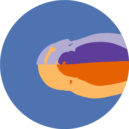


Legend: Clear-of-Conflict, Weak Right, Strong Right, Strong Left, Weak Left.
We have now seen how SyReNN can be used to visualize the behavior of a DNN. This can be particularly useful for identifying buggy behavior. For example, in Figure 3(a) we can see that the decision boundary between “strong right” and “strong left” is not symmetrical.
The final application we consider for SyReNN is patching DNNs to correct undesired behavior. Patching is described formally in [52]. Given an initial network and a specification describing desired constraints on the input/output, the goal of patching is to find a small modification to the parameters of producing a new DNN that satisfies the constraints in .
The key theory behind DNN patching we will use was developed in [52]. The key realization of that work is that, for a certain DNN architecture, correcting the network behavior on an infinite, 2D region is exactly equivalent to correcting its behavior on the finitely-many vertices for each of the finitely-many . Hence, SyReNN plays a key role in enabling efficient DNN patching.
For this case study, we patched the same aircraft collision-avoidance DNN visualized in Section 6.2. We patched the DNN three times to correct three different buggy behaviors of the network: (i) remove “Pockets” of strong left/strong right in regions that are otherwise weak left/weak right; (ii) remove the “Bands” of weak-left advisory behind and to the left of the plane; and (iii) enforce “Symmetry” across the horizontal. The DNNs before and after patching with different specifications are shown in Figure 4.
Implementation The helper class NetPatcher is provided by our Python client library. It takes as input a DNN and pairs of input region, output label , then computes a new DNN which maps all points in each into .
Timing Numbers. As in Section 6.2, computing for use in patching took approximately 10 seconds.
7 Related Work
The related problem of exact reach set analysis for DNNs was investigated in [59]. However, the authors use an algorithm that relies on explicitly enumerating all exponentially-many () possible signs at each ReLU layer. By contrast, our algorithm adapts to the actual input polytopes, efficiently restricting its consideration to activations that are actually possible.
Hanin and Rolnick [26] prove theoretical properties about the cardinality of for ReLU networks, showing that is expected to grow polynomially with the number of nodes in the network for randomly-initialized networks.
Thrun [56] and Bastani et al.[4] extract symbolic rules meant to approximate DNNs, which can be thought of as an approximation of the symbolic representation .
In particular, the ERAN [1] tool and underlying DeepPoly [50] domain were designed to verify the non-existence of adversarial examples. Breutel et al. [6] presents an iterative refinement algorithm that computes an overapproximation of the weakest precondition as a polytope where the required output is also a polytope.
Scheibler et al. [47] verify the safety of a machine-learning controller using the SMT-solver iSAT3, but support small unrolling depths and basic safety properties. Zhu et al. [61] use a synthesis procedure to generate a safe deterministic program that can enforce safety conditions by monitoring the deployed DNN and preventing potentially unsafe actions. The presence of adversarial and fooling inputs for DNNs as well as applications of DNNs in safety-critical systems has led to efforts to verify and certify DNNs [3, 33, 14, 30, 17, 7, 58, 50, 2]. Approximate reachability analysis for neural networks safely overapproximates the set of possible outputs [17, 59, 60, 58, 13, 57].
Prior work in the area of network patching focuses on enforcing constraints on the network during training. DiffAI [40] is an approach to train neural networks that are certifiably robust to adversarial perturbations. DL2 [15] allows for training and querying neural networks with logical constraints.
8 Conclusion and Future Work
We presented SyReNN, a tool for understanding and analyzing DNNs. Given a piecewise-linear network and a low-dimensional polytope subspace of the input subspace, SyReNN computes a symbolic representation that decomposes the behavior of the DNN into finitely-many linear functions. We showed how to efficiently compute this representation, and presented the design of the corresponding tool. We illustrated the utility of SyReNN on three applications: computing exact IG, visualizing the behavior of DNNs, and patching (repairing) DNNs.
In contrast to prior work, SyReNN explores a unique point in the design space of DNN analysis tools. In particular, instead of trading off precision of the analysis for efficiency, SyReNN focuses on analyzing DNN behavior on low-dimensional subspaces of the domain, for which we can provide both efficiency and precision.
We plan on extending SyReNN to make use of GPUs and other massively-parallel hardware to more quickly compute for large or . Techniques to support input polytopes that are greater than two dimensional is also a ripe area of future work. We may also be able to take advantage of the fact that non-convex polytopes can be represented efficiently in 2D. Extending algorithms for to handle architectures such as Recurrent Neural Networks (RNNs) will open up new application areas for SyReNN.
Acknowledgements.
We thank the anonymous reviewers for their feedback and suggestions on this work. This material is based upon work supported by a Facebook Probability and Programming award.
References
- [1] ETH robustness analyzer for neural networks (ERAN). https://github.com/eth-sri/eran (2019), accessed: 2019-05-01
- [2] Anderson, G., Pailoor, S., Dillig, I., Chaudhuri, S.: Optimization and abstraction: A synergistic approach for analyzing neural network robustness. CoRR abs/1904.09959 (2019)
- [3] Bastani, O., Ioannou, Y., Lampropoulos, L., Vytiniotis, D., Nori, A.V., Criminisi, A.: Measuring neural net robustness with constraints. In: Advances in Neural Information Processing Systems (2016)
- [4] Bastani, O., Pu, Y., Solar-Lezama, A.: Verifiable reinforcement learning via policy extraction. In: Advances in Neural Information Processing Systems 31: Annual Conference on Neural Information Processing Systems 2018, NeurIPS 2018, 3-8 December 2018, Montréal, Canada. pp. 2499–2509 (2018)
- [5] Beyer, D.: Reliable and reproducible competition results with benchexec and witnesses (report on sv-comp 2016). In: International Conference on Tools and Algorithms for the Construction and Analysis of Systems (TACAS). pp. 887–904. Springer (2016)
- [6] Breutel, S., Maire, F., Hayward, R.: Extracting interface assertions from neural networks in polyhedral format. In: ESANN 2003, 11th European Symposium on Artificial Neural Networks, Bruges, Belgium, April 23-25, 2003, Proceedings. pp. 463–468 (2003)
- [7] Bunel, R.R., Turkaslan, I., Torr, P.H.S., Kohli, P., Mudigonda, P.K.: A unified view of piecewise linear neural network verification. In: Advances in Neural Information Processing Systems 31: Annual Conference on Neural Information Processing Systems 2018, NeurIPS 2018, 3-8 December 2018, Montréal, Canada. pp. 4795–4804 (2018)
- [8] Carlini, N., Wagner, D.: Audio adversarial examples: Targeted attacks on speech-to-text. In: 2018 IEEE Security and Privacy Workshops (SPW). pp. 1–7. IEEE (2018)
- [9] Chen, J., Ran, X.: Deep learning with edge computing: A review. Proceedings of the IEEE 107(8), 1655–1674 (2019)
- [10] Ching, T., Himmelstein, D.S., Beaulieu-Jones, B.K., Kalinin, A.A., Do, B.T., Way, G.P., Ferrero, E., Agapow, P.M., Zietz, M., Hoffman, M.M., Xie, W., Rosen, G.L., Lengerich, B.J., Israeli, J., Lanchantin, J., Woloszynek, S., Carpenter, A.E., Shrikumar, A., Xu, J., Cofer, E.M., Lavender, C.A., Turaga, S.C., Alexandari, A.M., Lu, Z., Harris, D.J., DeCaprio, D., Qi, Y., Kundaje, A., Peng, Y., Wiley, L.K., Segler, M.H.S., Boca, S.M., Swamidass, S.J., Huang, A., Gitter, A., Greene, C.S.: Opportunities and obstacles for deep learning in biology and medicine. Journal of The Royal Society Interface 15(141), 20170387 (2018). https://doi.org/10.1098/rsif.2017.0387
- [11] Chollet, F., et al.: Keras. https://keras.io (2015)
- [12] Devlin, J., Chang, M., Lee, K., Toutanova, K.: BERT: pre-training of deep bidirectional transformers for language understanding. CoRR abs/1810.04805 (2018)
- [13] Dutta, S., Jha, S., Sankaranarayanan, S., Tiwari, A.: Output range analysis for deep feedforward neural networks. In: NASA Formal Methods Symposium. pp. 121–138. Springer (2018)
- [14] Ehlers, R.: Formal verification of piece-wise linear feed-forward neural networks. In: International Symposium on Automated Technology for Verification and Analysis (ATVA) (2017)
- [15] Fischer, M., Balunovic, M., Drachsler-Cohen, D., Gehr, T., Zhang, C., Vechev, M.: Dl2: Training and querying neural networks with logic. In: International Conference on Machine Learning (2019)
- [16] Fukuda, K., et al.: Frequently asked questions in polyhedral computation. ETH, Zurich, Switzerland (2004)
- [17] Gehr, T., Mirman, M., Drachsler-Cohen, D., Tsankov, P., Chaudhuri, S., Vechev, M.T.: AI2: safety and robustness certification of neural networks with abstract interpretation. In: 2018 IEEE Symposium on Security and Privacy, SP 2018, Proceedings, 21-23 May 2018, San Francisco, California, USA (2018)
- [18] Gonzales, R.: Feds say self-driving uber suv did not recognize jaywalking pedestrian in fatal crash. NPR https://www.npr.org/2019/11/07/777438412/feds-say-self-driving-uber-suv-did-not-recognize-jaywalking-pedestrian-in-fatal- (Nov 2019), accessed: 2020-06-06
- [19] Goodfellow, I., Bengio, Y., Courville, A.: Deep Learning. MIT Press (2016), http://www.deeplearningbook.org
- [20] Goodfellow, I.J., Shlens, J., Szegedy, C.: Explaining and harnessing adversarial examples. In: International Conference on Learning Representations, ICLR (2015)
- [21] Google: grpc: A high-performance, open source universal rpc framework. ”https://grpc.io/ (2020)
- [22] Google: Protocol buffers - google’s data interchange format. https://developers.google.com/protocol-buffers/ (2020)
- [23] Gopinath, S., Ghanathe, N., Seshadri, V., Sharma, R.: Compiling kb-sized machine learning models to tiny iot devices. In: Proceedings of the 40th ACM SIGPLAN Conference on Programming Language Design and Implementation, PLDI. pp. 79–95. ACM (2019)
- [24] Guennebaud, G., Jacob, B., et al.: Eigen v3. http://eigen.tuxfamily.org (2010)
- [25] Han, S., Mao, H., Dally, W.J.: Deep compression: Compressing deep neural networks with pruning, trained quantization and huffman coding. International Conference on Learning Representations (ICLR) (2016)
- [26] Hanin, B., Rolnick, D.: Complexity of linear regions in deep networks. International Conference on Machine Learning (ICML) (2019)
- [27] Hern, A.: Facebook translates ’good morning’ into ’attack them’, leading to arrest. https://www.theguardian.com/technology/2017/oct/24/facebook-palestine-israel-translates-good-morning-attack-them-arrest (Jun 2017), accessed: 2020-06-06
- [28] Hill, K.: Wrongfully accused by an algorithm. New York Times. https://www.nytimes.com/2020/06/24/technology/facial-recognition-arrest.html (Jun 2020), accessed: 2020-06-06
- [29] Hosny, A., Parmar, C., Quackenbush, J., Schwartz, L.H., Aerts, H.J.: Artificial intelligence in radiology. Nature Reviews Cancer p. 1 (2018)
- [30] Huang, X., Kwiatkowska, M., Wang, S., Wu, M.: Safety verification of deep neural networks. In: International Conference on Computer Aided Verification (CAV) (2017)
- [31] Jeannet, B., Miné, A.: Apron: A library of numerical abstract domains for static analysis. In: International Conference on Computer Aided Verification (CAV). pp. 661–667. Springer (2009)
- [32] Julian, K.D., Kochenderfer, M.J., Owen, M.P.: Deep neural network compression for aircraft collision avoidance systems. Journal of Guidance, Control, and Dynamics 42(3), 598–608 (2018)
- [33] Katz, G., Barrett, C., Dill, D.L., Julian, K., Kochenderfer, M.J.: Reluplex: An efficient smt solver for verifying deep neural networks. In: International Conference on Computer Aided Verification (CAV) (2017)
- [34] Krizhevsky, A., Sutskever, I., Hinton, G.E.: Imagenet classification with deep convolutional neural networks. Commun. ACM 60(6), 84–90 (2017)
- [35] Kumar, A., Seshadri, V., Sharma, R.: Shiftry: Rnn inference in 2kb of ram. In: International Conference on Object-Oriented Programming, Systems, Languages, and Applications, OOPSLA (2020)
- [36] Kusupati, A., Singh, M., Bhatia, K., Kumar, A., Jain, P., Varma, M.: Fastgrnn: A fast, accurate, stable and tiny kilobyte sized gated recurrent neural network. In: Advances in Neural Information Processing Systems. pp. 9017–9028 (2018)
- [37] Lee, D.: US opens investigation into Tesla after fatal crash. BBC. https://www.bbc.co.uk/news/technology-36680043 (Jul 2016), accessed: 2020-06-06
- [38] Mendelson, E.B.: Artificial intelligence in breast imaging: potentials and limitations. American Journal of Roentgenology 212(2), 293–299 (2019)
- [39] Miotto, R., Wang, F., Wang, S., Jiang, X., Dudley, J.T.: Deep learning for healthcare: review, opportunities and challenges. Briefings in Bioinformatics 19(6), 1236–1246 (2018)
- [40] Mirman, M., Gehr, T., Vechev, M.: Differentiable abstract interpretation for provably robust neural networks. In: International Conference on Machine Learning ICML (2018)
- [41] Moosavi-Dezfooli, S., Fawzi, A., Frossard, P.: Deepfool: A simple and accurate method to fool deep neural networks. In: 2016 IEEE Conference on Computer Vision and Pattern Recognition, CVPR 2016, Las Vegas, NV, USA, June 27-30, 2016. pp. 2574–2582 (2016)
- [42] Nguyen, A.M., Yosinski, J., Clune, J.: Deep neural networks are easily fooled: High confidence predictions for unrecognizable images. In: IEEE Conference on Computer Vision and Pattern Recognition, (CVPR) 2015, Boston, MA, USA, June 7-12, 2015. pp. 427–436 (2015)
- [43] ONNX: Open neural network exchange. https://onnx.ai/ (2020)
- [44] Paszke, A., Gross, S., Chintala, S., Chanan, G., Yang, E., DeVito, Z., Lin, Z., Desmaison, A., Antiga, L., Lerer, A.: Automatic differentiation in pytorch (2017)
- [45] Paszke, A., Gross, S., Massa, F., Lerer, A., Bradbury, J., Chanan, G., Killeen, T., Lin, Z., Gimelshein, N., Antiga, L., Desmaison, A., Kopf, A., Yang, E., DeVito, Z., Raison, M., Tejani, A., Chilamkurthy, S., Steiner, B., Fang, L., Bai, J., Chintala, S.: Pytorch: An imperative style, high-performance deep learning library. In: Wallach, H., Larochelle, H., Beygelzimer, A., d’ Alché-Buc, F., Fox, E., Garnett, R. (eds.) Advances in Neural Information Processing Systems 32, pp. 8024–8035. Curran Associates, Inc. (2019), http://papers.nips.cc/paper/9015-pytorch-an-imperative-style-high-performance-deep-learning-library.pdf
- [46] Reinders, J.: Intel threading building blocks: outfitting C++ for multi-core processor parallelism. ” O’Reilly Media, Inc.” (2007)
- [47] Scheibler, K., Winterer, L., Wimmer, R., Becker, B.: Towards verification of artificial neural networks. In: Methoden und Beschreibungssprachen zur Modellierung und Verifikation von Schaltungen und Systemen, MBMV 2015, Chemnitz, Germany, March 3-4, 2015. pp. 30–40 (2015)
- [48] Sharma, H., Park, J., Mahajan, D., Amaro, E., Kim, J.K., Shao, C., Mishra, A., Esmaeilzadeh, H.: From high-level deep neural models to fpgas. In: 2016 49th Annual IEEE/ACM International Symposium on Microarchitecture (MICRO). pp. 1–12. IEEE (2016)
- [49] Singh, G., Gehr, T., Mirman, M., Püschel, M., Vechev, M.: Fast and effective robustness certification. In: Advances in Neural Information Processing Systems (2018)
- [50] Singh, G., Gehr, T., Püschel, M., Vechev, M.T.: An abstract domain for certifying neural networks. PACMPL 3(POPL), 41:1–41:30 (2019)
- [51] Sotoudeh, M., Thakur, A.V.: Computing linear restrictions of neural networks. In: Advances in Neural Information Processing Systems 32: Annual Conference on Neural Information Processing Systems 2019, NeurIPS 2019, 8-14 December 2019, Vancouver, BC, Canada. pp. 14132–14143 (2019)
- [52] Sotoudeh, M., Thakur, A.V.: Correcting deep neural networks with small, generalizing patches. In: Workshop on Safety and Robustness in Decision Making (2019)
- [53] Sundararajan, M., Taly, A., Yan, Q.: Axiomatic attribution for deep networks. In: International Conference on Machine Learning ICML (2017)
- [54] Szegedy, C., Vanhoucke, V., Ioffe, S., Shlens, J., Wojna, Z.: Rethinking the inception architecture for computer vision. In: Proceedings of the IEEE conference on computer vision and pattern recognition (CVPR) (2016)
- [55] Szegedy, C., Zaremba, W., Sutskever, I., Bruna, J., Erhan, D., Goodfellow, I.J., Fergus, R.: Intriguing properties of neural networks. In: International Conference on Learning Representations, ICLR (2014)
- [56] Thrun, S.: Extracting rules from artifical neural networks with distributed representations. In: Advances in Neural Information Processing Systems 7, [NIPS Conference, Denver, Colorado, USA, 1994]. pp. 505–512 (1994)
- [57] Wang, S., Pei, K., Whitehouse, J., Yang, J., Jana, S.: Formal security analysis of neural networks using symbolic intervals. In: 27th USENIX Security Symposium, USENIX Security 2018, Baltimore, MD, USA, August 15-17, 2018. pp. 1599–1614 (2018)
- [58] Weng, T., Zhang, H., Chen, H., Song, Z., Hsieh, C., Daniel, L., Boning, D.S., Dhillon, I.S.: Towards fast computation of certified robustness for relu networks. In: International Conference on Machine Learning, (ICML) (2018)
- [59] Xiang, W., Tran, H.D., Johnson, T.T.: Reachable set computation and safety verification for neural networks with relu activations. arXiv preprint arXiv:1712.08163 (2017)
- [60] Xiang, W., Tran, H., Rosenfeld, J.A., Johnson, T.T.: Reachable set estimation and safety verification for piecewise linear systems with neural network controllers. In: 2018 Annual American Control Conference, (ACC) (2018)
- [61] Zhu, H., Xiong, Z., Magill, S., Jagannathan, S.: An inductive synthesis framework for verifiable reinforcement learning. In: Proceedings of the 40th ACM SIGPLAN Conference on Programming Language Design and Implementation, PLDI 2019, Phoenix, AZ, USA, June 22-26, 2019. pp. 686–701 (2019)
Open Access This chapter is licensed under the terms of the Creative CommonsAttribution 4.0 International License (https://creativecommons.org/licenses/by/4.0/), which permits use, sharing, adaptation, distribution and reproduction in any medium or format, as long as you give appropriate credit to the original author(s) and the source, provide a link to the Creative Commons license and indicate if changes were made.
The images or other third party material in this chapter are included in the chapter’s Creative Commons license, unless indicated otherwise in a credit line to the material. If material is not included in the chapter’s Creative Commons license and your intendeduse is not permitted by statutory regulation or exceeds the permitted use, you will need to obtain permission directly from the copyright holder.
![[Uncaptioned image]](2101.03263v1/cc_by_4-0.png)