Autoheterodyne characterization of narrow-band photon pairs

Spontaneous parametric downconversion (SPDC) is a ubiquitous technique in photonic quantum technology, where it is used to generate entangled photons with tailored spectral, spatial, and polarization properties Couteau 2018. The frequency correlations of SPDC photon pairs, including time-frequency entanglement, are of particular importance. In some applications these correlations are used to encode quantum information Reimer et al. 2019; Pfister 2019. In others, the frequency correlations are an undesired side-channel that reduces nonclassical interference Gerrits et al. 2015. These correlations are revealed through analysis of the joint spectral amplitude (JSA) or joint spectral intensity (JSI) of the downconverted photon pair.

In broadband SPDC applications, it is possible to directly measure the JSI using monochromators or other passive filters Kim and Grice 2005; Zielnicki et al. 2018. Techniques such as Fourier transform spectroscopy using Mach Zehnder interferometers Wasilewski et al. 2006 and temporal magnification of photons with a time lens Mittal et al. 2017 have also been used. Non-classical interference can also be a tool to characterize non-classical frequency correlations; the Hong-Ou-Mandel (HOM) Hong et al. 1987 interference visibility has been used to characterize broadband photon pairs from a single source Gerrits et al. 2015; Gerrits et al. 2011; Zielnicki et al. 2018 and from different sources Wang et al. 2019; Thiel et al. 2020.

Photon pairs with $\sim$\text{\,}\mathrm{MHz}$$ bandwidths are important for applications in quantum information Slattery et al. 2019 where material systems such as atoms or ions serve as storage or processing units Distante et al. 2017; Seri et al. 2017. For example, sub-wavelength arrays of neutral atoms support sub-radiant states Asenjo-Garcia et al. 2017 that can exhibit topological protection Perczel et al. 2017 and unprecedented optical properties Rui et al. 2020. Strong photon-photon interactions Masson and Asenjo-Garcia 2020 that could be harnessed for photonic quantum-information processing, and photonic bound states Deutsch et al. 1992; Ke et al. 2020 are predicted in such arrays. Exploring this physics motivates non-classical light sources in which both photons are resonant to an atomic transition Prakash et al. 2019. Applications in quantum networking, e.g. entanglement-swapping with memory-compatible photons, will require pure, indistinguishable, narrowband photons Monteiro et al. 2014.

Such narrow-band photon pairs are not easily measured by passive frequency-domain techniques, because of the very high optical frequency resolution it would require. In such a two-photon Fock state, first-order interference vanishes, producing no observable beat note Note1. One alternative is stimulated parametric downconversion Liscidini and Sipe 2013, in which laser photons are used to seed the downconversion and map the difference frequencies generated vs those suppressed Jeong and Moon 2020; Prakash et al. 2019. This technique has potential for use in tomography of the JSA Jizan et al. 2016, but requires an additional well-characterized laser source and careful matching of spatial modes.

Here we present a simpler and more efficient alternative, a time-domain characterization of the two-photon state using non-classical interference. The JSI is a two-dimensional function, while the HOM interference visibility is a scalar observable. Thus a characterisation of the JSI even along a single dimension requires many HOM visibility measurements under changing experimental conditions, such as a changing path length Ou and Mandel 1988; Jin and Shimizu 2018. In contrast, the Ghosh and Mandel experiment Ghosh and Mandel 1987 (GM), which measured the spatial interference pattern produced by photons of unequal momentum, showed how a correlation spectrum can be acquired with a single experimental condition. This motivates us to look for techniques that give more direct and more efficient access to the frequency correlations of interest. Our proposals for narrow-band photon pair characterization, are extensions of the HOM and GM interference effects.

The principle of the method is illustrated in Figure 1. Narrow-band photon pairs with the photons of each pair matched in polarization and spatial profile but with unequal frequency, are injected, one into port $A$ and the other into port $B$ of a 50/50 beamsplitter (BS). Single-photon-sensitive detectors register photons leaving the BS by ports $C$ and $D$, and time-tagging electronics record the arrival times. Many events are accumulated, and the second order correlation functions $G^{(2)}_{\kappa,\mu}(t,t^{\prime})$, $\kappa,\mu\in\{C,D\}$ are calculated. Information about the JSA can then be inferred from the $G^{(2)}$ functions. We refer to this method as auto-heterodyne characterization (AHC), not to be confused with the single-photon self-heterodyne technique Okawa et al. 2017.

When photons of different frequency meet at a BS, their arrival-time distribution becomes modulated at the difference of their frequencies. This can be understood as follows: a detection at $C$ and $D$ with zero time delay, i.e. $t=t^{\prime}$, can happen by two channels in configuration space: either reflection of both photons or transmission of both photons. The amplitudes for these channels sum to zero, due to phase factors in the transmission and reflection processes. The resulting vanishing of $G^{(2)}_{C,D}(t,t)$ and the corresponding increase of $G^{(2)}_{C,C}(t,t)$ and $G^{(2)}_{D,D}(t,t)$ is the well-known HOM effect Hong et al. 1987. For unequal detection times, one must also consider the phase factors $\exp[-i\omega_{A}t-i\omega_{B}t^{\prime}]$ and $\exp[-i\omega_{A}t^{\prime}-i\omega_{B}t]$ that apply to the two-reflection and two-transmission channels, respectively. The relative phase $(\omega_{A}-\omega_{B})(t-t^{\prime})$ between the channels then induces an oscillation of the $G^{(2)}$ correlations at the difference frequency $\omega_{A}-\omega_{B}$. We refer to this non-classical interference between distinguishable photons as the non-degenerate HOM effect. Small frequency differences between the photons manifest as long-period oscillations in the relative arrival time distribution, which are technologically convenient to detect.

The effect can be easily calculated. For a two-photon input state $\left|\psi\right>$ with JSA $f(\omega_{A},\omega_{B})$,

The un-normalised correlation functions are $G^{(2)}_{\alpha,\beta}(t,t^{\prime})\equiv|\langle 0|\hat{E}^{(+)}_{\alpha}(t)\hat{E}^{(+)}_{\beta}(t^{\prime})|\psi\rangle|^{2}$, $\alpha,\beta\in\{A,B,C,D\}$, where the field operators are $\hat{E}^{(+)}_{\alpha}(t)\propto\int d\omega\hat{a}_{\alpha}(\omega)\exp[{-i\omega t}]$ and $\hat{a}_{\alpha}$ is an annihilation operator. Due to the beamsplitter, the output fields are $\hat{E}^{(+)}_{C/D}(t)\propto\hat{E}^{(+)}_{A}(t)\pm\hat{E}^{(+)}_{B}(t)$. A straightforward calculation finds

where $\omega_{\pm}\equiv\omega_{A}\pm\omega_{B}$, $t_{\pm}\equiv t\pm t^{\prime}$ and the integral is taken over $\omega_{A},\omega_{B}$ or equivalently over $\omega_{+},\omega_{-}$, with $\vec{\omega}$ being the corresponding parametrization of $f$ and $\osc\theta=\frac{1}{\sqrt{2}}\cos\theta$ if $\kappa,\mu=C,C$ or $D,D$ and $i\sin\theta$ otherwise. This describes a Fourier transform of the JSA along the $\omega_{\pm}$ coordinates. When the two-photon state is produced by SPDC, and pumped by a broadband pump with field $E_{p}(t)=\int d\omega_{p}\alpha(\omega_{p})e^{-i\omega_{p}t}$, $f\propto\int d\omega_{p}\alpha(\omega_{p})\delta(\omega_{p}-\omega_{+})g(\omega_{-},\omega_{+})\propto\alpha(\omega_{+})g(\omega_{-},\omega_{+})$. When the variation of the crystal phase matching function over the pump-bandwidth can be neglected, $g$ becomes independent of $\omega_{+}$ and the JSA factorizes as $f\propto\alpha(\omega_{+})g(\omega_{-})$. The $G^{(2)}$ then gives the sine or cosine power spectrum of $g(\omega_{-})$ in the $t_{-}$ dimension and also gives the Fourier transformed spectrum of $\alpha(\omega_{+})$ via the $t_{+}$ dimension ¹¹ 1 See Supplemental Material for application of AHC to heralded pure state characterisation, calculations relating the power spectral density of the AHC $G^{(2)}$ to the JSA, discussions related to the resolution of AHC and first order interference effects from single photon states.. For a monochromatic pump $\alpha(\omega_{+})\rightarrow\delta(\omega_{+}-\omega_{p})$, such that $f\propto\delta(\omega_{+}-\omega_{p})g(\omega_{-})$, and $G^{(2)}$ depends only on $t_{-}$. In what follows we study the narrowband, cw-pump case. The use of AHC in the pulsed scenario and to obtain measures such as entanglement entropy, state purity and Schmidt number Brańczyk et al. 2010 is discussed in the Supplemental Material Note1

We note that this technique implements a variant of the GM effect Ghosh and Mandel 1987. In GM, photon pairs with unequal transverse momenta $k_{s},k_{i}$ are observed to produce a spatial auto-correlation function $G^{(2)}(x-x^{\prime})$ that is maximum for $x-x^{\prime}=0$ and modulated with momentum $k_{s}-k_{i}$. The temporal modulation of $G^{(2)}_{C,C}$ or $G^{(2)}_{D,D}$, which describes the correlations of photon pairs with unequal frequencies $\omega_{A},\omega_{B}$ in a single output channel, is the temporal analog of GM. We refer to this as the temporal Ghosh-Mandel effect. By conservation of probability at the BS, the GM and HOM signals must add to give $G^{(2)}_{A,B}(t,t^{\prime})$, as illustrated in Figure 1. As a result, the two methods give very similar information about the JSA.

To demonstrate this experimentally, we use photon pairs from a cavity-enhanced SPDC (CE-SPDC) source pumped by a single-frequency laser. The experimental setup is shown schematically in Fig. 2. Photon pairs are produced by a narrow-band CE-SPDC source, described in detail in Prakash et al. 2019. A pump laser at $397.5\text{\,}\mathrm{nm}$ with full width half-maximum (FWHM) linewidth $\approx$2\text{\,}\mathrm{MHz}$$ pumps a type-II periodically-poled Potassium Titanyl Phosphate (PPKTP) crystal to produce photon pairs of orthogonal linear polarization. The cavity mode structure, with signal and idler free-spectral range (FSR_s and FSR_i) $\approx$500\text{\,}\mathrm{MHz}$$ and FWHM linewidth $\gamma=2\pi\times$7.6\text{\,}\mathrm{MHz}$$ for both $H$ (signal - $s$) and $V$ (idler - $i$) polarizations, shapes the output spectrum by the Purcell effect. Birefringent crystals in the SPDC cavity produce a mismatch of $\Delta$FSR = $3.5\text{\,}\mathrm{MHz}$ in the FSRs of the signal and idler modes. This reduces the number of modes at the output to 3 clusters of 4 modes each for a downconversion crystal bandwidth of $150\text{\,}\mathrm{GHz}$ as shown in Prakash et al. 2019. The contribution of unwanted modes is blocked by a pair of tuneable Fabry-Perot (FP) filters with linewidth $\gamma_{f}=2\pi\times$97\text{\,}\mathrm{MHz}$$ and FSR${}_{f}=$39\text{\,}\mathrm{GHz}$$.

To perform AHC of the CE-SPDC source, the pump laser, cavity mode and FP mode frequencies are tuned to produce and pass a single signal-idler mode pair within the $794.7\text{\,}\mathrm{nm}$ D₁ line of atomic Rb, with frequency difference $\omega^{0}_{-}=\omega^{0}_{s}-\omega^{0}_{i}$, between the central frequencies. The measurement is performed for two values of $\omega^{0}_{-}/(2\pi)$, $250\text{\,}\mathrm{MHz}$ and $165\text{\,}\mathrm{MHz}$. Single-mode fibers and linear polarizers ensure good spatial and polarization matching when the signal and idler photons arrive at the BS via spatial modes $A$ and $B$, respectively. BS output modes $C$ and $D$ are coupled into single mode fibers leading to avalanche photodiodes (APDs, Perkin Elmer SPCM-AQ4C, quantum efficiency $\approx$50\text{\,}\mathrm{\%}$$). A field programmable gate array (FPGA) records all APD firings with a resolution of $625\text{\,}\mathrm{ps}$ (sampling rate $1.6\text{\,}\mathrm{GHz}$).

The two-photon state at the output of a CE-SPDC system when pumped by a cw laser of frequency $\omega_{p}$ is given by Equation 1 with $\omega_{A/B}\rightarrow\omega_{s/i}$, $f\rightarrow f^{\prime}$ and

where $F(\omega_{s},\omega_{i})$ is the collinear phase-matching amplitude for the SPDC process and the delta function imposes energy conservation Scholz et al. 2009. For $\nu\in{s,i}$,

where the mode index $m$ is summed over positive and negative integers. In practice, the summations can be truncated to cover only those values for which $F(\omega_{s},\omega_{i})$ is significant.

When FP cavities are used to filter the multimode CE-SPDC output, the two-photon JSA after the filters is

If the FP filters are tuned to the preferred CE-SPDC output modes as described above, the filters’ index frequencies coincide with those of the CE-SPDC cavity, i.e., $\omega^{0}_{f_{\nu}}=\omega^{0}_{\nu}$. In this case, the JSA for our FP and CE-SPDC linewidths and FSRs, is well approximated by a Lorentzian each for the signal and idler

When inserted into Equation S3, we find

Figure 3a) shows the observed and predicted $G^{(2)}_{C,D}$ for a frequency difference of $\omega^{0}_{-}=2\pi\times$250\text{\,}\mathrm{MHz}$$ between the signal and idler modes. In accordance with the theory, the results show a clear oscillation with period $4\text{\,}\mathrm{ns}$, the inverse of $250\text{\,}\mathrm{MHz}$. The visibility of the interference is 82$\%$, which is greater than the classical limit of 50$\%$ Ghosh and Mandel 1987, attests to the fact that the interference was produced by non-classical states. The predicted $G^{(2)}_{C,D}$, calculated with $\gamma=2\pi\times$7.6\text{\,}\mathrm{MHz}$$, agrees with the observed fringe period and also with the decay rate of the exponential envelope. Equation S15 implies a FWHM bandwidth of $\gamma\sqrt{\sqrt{2}-1}=2\pi\times$4.9\text{\,}\mathrm{MHz}$$ for signal, idler, and difference frequency Scholz et al. 2009. The AHC measurement was repeated for a signal-idler frequency difference of $165\text{\,}\mathrm{MHz}$, and thus an oscillation period $\approx$6\text{\,}\mathrm{ns}$$ in $G^{(2)}_{C,D}$.

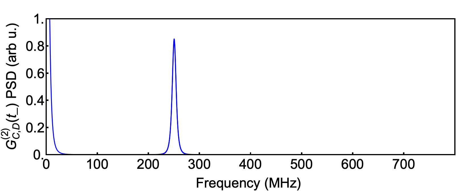
The power spectra of the observed $G^{(2)}_{C,D}$ for $\omega^{0}_{-}/2\pi$ of $250\text{\,}\mathrm{MHz}$ and $165\text{\,}\mathrm{MHz}$ are shown in Figure 3b) and 3c) respectively. Each shows a peak at dc and a Lorentzian peak at the corresponding $\omega^{0}_{-}$, of the same width and center frequency as the Lorentzian in the JSI computed from Equation S15 Note1. The resolution of these spectra is inversely proportional to the range of $t-t^{\prime}$, which can extend to the full acquisition time. In practice, the resolution is much finer than any spectral feature. The spectral range, i.e. the largest observable difference frequency, is set by the time resolution of the detection. With few-ps detection Korzh et al. 2020, a difference-frequency range of $\sim$100\text{\,}\mathrm{GHz}$$ can be achieved Note1.

Inefficient extinction of neighbouring CE-SPDC modes by the FP filter would manifest as additional signals in the PSD besides one at the expected $\omega_{-}^{0}$. In Figure 3b), peaks at $750\text{\,}\mathrm{MHz}$ and/or $350\text{\,}\mathrm{MHz}$ (aliased down from $1250\text{\,}\mathrm{MHz}$ due to the sampling rate of the FPGA) would indicate leakage of mode pairs with $\omega_{-}/2\pi=$250\text{\,}\mathrm{MHz}$\pm 2\,\mathrm{FSR}$ (red arrows). A peak at $500\text{\,}\mathrm{MHz}$ (the FSR for both signal and idler) might also be expected, but is not seen (orange arrow). Similarly, leakage would produce peaks at $765\text{\,}\mathrm{MHz}$ and $435\text{\,}\mathrm{MHz}$ (red arrows), and again $500\text{\,}\mathrm{MHz}$ (orange arrow) in Figure 3c). We thus conclude that the FP cavity filtering succeeds in blocking contributions from neighbouring CE-SPDC modes and that the combined CE-SPDC and filter system emits on one pair of CE-SPDC cavity modes.

Measurement of $G^{(2)}_{C,C}$, showing the temporal GM effect, is shown in Figure 4 for $\omega^{0}_{-}=2\pi\times$250\text{\,}\mathrm{MHz}$$. Typically SPDC $G^{(2)}$ autocorrelations require a BS and two detectors, in order to record photon pairs that arrive spaced by less than a detector’s dead time, here $\approx$40\text{\,}\mathrm{ns}$$. For narrow-band photon pairs, however, it is possible to acquire the autocorrelation with just one detector, as we do here. The predicted oscillation with a period of $4\text{\,}\mathrm{ns}$ is clearly observed. The temporal GM effect thus offers a simple way to characterize relative frequencies with a single detector. Frequency-shifting of one input photon through nonlinear-optical frequency conversion Maring et al. 2018, would allow AHC to measure spectra with difference frequencies outside the the detection electronics’ bandwidth.

We have demonstrated a new technique to quantify the frequency correlations of narrow-band photon pairs and applied it to measure the spectral content of a filtered, cavity-enhanced parametric downconversion source at the Rb D₁ line with $\approx$5\text{\,}\mathrm{MHz}$$ optical bandwidth. By interfering the photons on a BS and performing Fourier analysis on the temporal auto- and cross-correlations, AHC directly measures the beat-note spectrum with the spectral resolution limited only by the acquisition time. The technique is simple to implement with one detector via the temporal Ghosh-Mandel effect, or with two detectors via the non-degenerate Hong-Ou-Mandel effect. It is well suited to characterize narrow-band photon sources for interaction with atoms and ions, which typically require bandwidths below $10\text{\,}\mathrm{MHz}$. The technique may be especially valuable in quantum networking, computing and simulation with mixed photon-atom systems.

We thank Dr. Robert Sewell, Samyobrata Mukherjee and Natália Alves for feedback on the manuscript. This project was supported by H2020 Future and Emerging Technologies Quantum Technologies Flagship project QRANGE (Grant Agreement No. 820405); Spanish MINECO projects OCARINA (Grant No. PGC2018-097056-B-I00), Q-CLOCKS (Grant No. PCI2018-092973), and the Severo Ochoa program (Grant No. SEV-2015-0522); Generalitat de Catalunya through the CERCA program; Agència de Gestió d’Ajuts Universitaris i de Recerca Grant No. 2017-SGR-1354; Secretaria d’Universitats i Recerca del Departament d’Empresa i Coneixement de la Generalitat de Catalunya, co-funded by the European Union Regional Development Fund within the ERDF Operational Program of Catalunya (project QuantumCat, ref. 001-P-001644); Fundació Privada Cellex; Fundació Mir-Puig; European Union’s H2020 Marie Skłodowska-Curie Actions (665884). National Science Centre, Poland (2018/28/T/ST2/00275 and 2019/34/E/ST2/00440).

Supplementary Material for
Autoheterodyne Characterization of Narrow-Band Photon Pairs

References

- Couteau (2018) C. Couteau, Contemporary Physics 59, 291 (2018).
- Reimer et al. (2019) C. Reimer, S. Sciara, P. Roztocki, M. Islam, L. Romero Cortés, Y. Zhang, B. Fischer, S. Loranger, R. Kashyap, A. Cino, S. T. Chu, B. E. Little, D. J. Moss, L. Caspani, W. J. Munro, J. Azaña, M. Kues, and R. Morandotti, Nature Physics 15, 148 (2019).
- Pfister (2019) O. Pfister, Journal of Physics B: Atomic, Molecular and Optical Physics 53, 012001 (2019).
- Gerrits et al. (2015) T. Gerrits, F. Marsili, V. B. Verma, L. K. Shalm, M. Shaw, R. P. Mirin, and S. W. Nam, Phys. Rev. A 91, 013830 (2015).
- Kim and Grice (2005) Y.-H. Kim and W. P. Grice, Opt. Lett. 30, 908 (2005).
- Zielnicki et al. (2018) K. Zielnicki, K. Garay-Palmett, D. Cruz-Delgado, H. Cruz-Ramirez, M. F. O’Boyle, B. Fang, V. O. Lorenz, A. B. U’Ren, and P. G. Kwiat, Journal of Modern Optics 65, 1141 (2018).
- Wasilewski et al. (2006) W. Wasilewski, P. Wasylczyk, P. Kolenderski, K. Banaszek, and C. Radzewicz, Opt. Lett. 31, 1130 (2006).
- Mittal et al. (2017) S. Mittal, V. V. Orre, A. Restelli, R. Salem, E. A. Goldschmidt, and M. Hafezi, Phys. Rev. A 96, 043807 (2017).
- Hong et al. (1987) C. K. Hong, Z. Y. Ou, and L. Mandel, Phys. Rev. Lett. 59, 2044 (1987).
- Gerrits et al. (2011) T. Gerrits, M. J. Stevens, B. Baek, B. Calkins, A. Lita, S. Glancy, E. Knill, S. W. Nam, R. P. Mirin, R. H. Hadfield, R. S. Bennink, W. P. Grice, S. Dorenbos, T. Zijlstra, T. Klapwijk, and V. Zwiller, Opt. Express 19, 24434 (2011).
- Wang et al. (2019) S. Wang, C.-X. Liu, J. Li, and Q. Wang, Scientific Reports 9, 3854 (2019).
- Thiel et al. (2020) V. Thiel, A. O. C. Davis, K. Sun, P. D’Ornellas, X.-M. Jin, and B. J. Smith, Opt. Express 28, 19315 (2020).
- Slattery et al. (2019) O. Slattery, L. Ma, K. Zong, and X. Tang, Journal of Research of the National Institute of Standards and Technology 124, 1 (2019).
- Distante et al. (2017) E. Distante, P. Farrera, A. Padrón-Brito, D. Paredes-Barato, G. Heinze, and H. de Riedmatten, Nature Communications 8, 14072 (2017).
- Seri et al. (2017) A. Seri, A. Lenhard, D. Rieländer, M. Gündoğan, P. M. Ledingham, M. Mazzera, and H. de Riedmatten, Phys. Rev. X 7, 021028 (2017).
- Asenjo-Garcia et al. (2017) A. Asenjo-Garcia, M. Moreno-Cardoner, A. Albrecht, H. J. Kimble, and D. E. Chang, Phys. Rev. X 7, 031024 (2017).
- Perczel et al. (2017) J. Perczel, J. Borregaard, D. E. Chang, H. Pichler, S. F. Yelin, P. Zoller, and M. D. Lukin, Physical Review Letters 119, 023603 (2017).
- Rui et al. (2020) J. Rui, D. Wei, A. Rubio-Abadal, S. Hollerith, J. Zeiher, D. M. Stamper-Kurn, C. Gross, and I. Bloch, Nature 583, 369 (2020).
- Masson and Asenjo-Garcia (2020) S. J. Masson and A. Asenjo-Garcia, Phys. Rev. Research 2, 043213 (2020).
- Deutsch et al. (1992) I. H. Deutsch, R. Y. Chiao, and J. C. Garrison, Phys. Rev. Lett. 69, 3627 (1992).
- Ke et al. (2020) Y. Ke, J. Zhong, A. V. Poshakinskiy, Y. S. Kivshar, A. N. Poddubny, and C. Lee, Phys. Rev. Research 2, 033190 (2020).
- Prakash et al. (2019) V. Prakash, L. C. Bianchet, M. T. Cuairan, P. Gomez, N. Bruno, and M. W. Mitchell, Opt. Express 27, 38463 (2019).
- Monteiro et al. (2014) F. Monteiro, A. Martin, B. Sanguinetti, H. Zbinden, and R. T. Thew, Opt. Express 22, 4371 (2014).
- (24) See Supplemental Material for application of AHC to heralded pure state characterisation, calculations relating the power spectral density of the AHC to the JSA, discussions related to the resolution of AHC and first order interference effects from single photon states.
- Liscidini and Sipe (2013) M. Liscidini and J. E. Sipe, Phys. Rev. Lett. 111, 193602 (2013).
- Jeong and Moon (2020) T. Jeong and H. S. Moon, Opt. Lett. 45, 2668 (2020).
- Jizan et al. (2016) I. Jizan, B. Bell, L. G. Helt, A. C. Bedoya, C. Xiong, and B. J. Eggleton, Opt. Lett. 41, 4803 (2016).
- Ou and Mandel (1988) Z. Y. Ou and L. Mandel, Phys. Rev. Lett. 61, 54 (1988).
- Jin and Shimizu (2018) R.-B. Jin and R. Shimizu, Optica 5, 93 (2018).
- Ghosh and Mandel (1987) R. Ghosh and L. Mandel, Phys. Rev. Lett. 59, 1903 (1987).
- Okawa et al. (2017) Y. Okawa, F. Omura, Y. Yasutake, and S. Fukatsu, Opt. Express 25, 20156 (2017).
- Brańczyk et al. (2010) A. M. Brańczyk, T. C. Ralph, W. Helwig, and C. Silberhorn, New Journal of Physics 12, 063001 (2010).
- Scholz et al. (2009) M. Scholz, L. Koch, and O. Benson, Optics Communications 282, 3518 (2009).
- Korzh et al. (2020) B. Korzh, Q.-Y. Zhao, J. P. Allmaras, S. Frasca, T. M. Autry, E. A. Bersin, A. D. Beyer, R. M. Briggs, B. Bumble, M. Colangelo, G. M. Crouch, A. E. Dane, T. Gerrits, A. E. Lita, F. Marsili, G. Moody, C. Peña, E. Ramirez, J. D. Rezac, N. Sinclair, M. J. Stevens, A. E. Velasco, V. B. Verma, E. E. Wollman, S. Xie, D. Zhu, P. D. Hale, M. Spiropulu, K. L. Silverman, R. P. Mirin, S. W. Nam, A. G. Kozorezov, M. D. Shaw, and K. K. Berggren, Nature Photonics 14, 250 (2020).
- Maring et al. (2018) N. Maring, D. Lago-Rivera, A. Lenhard, G. Heinze, and H. de Riedmatten, Optica 5, 507 (2018).