Market Making with Stochastic Liquidity Demand:
Simultaneous Order Arrival and Price Change Forecasts

Since the last decade, most security trading activities have migrated to electronic markets and, as a result, high frequency trading has become one of the most significant market developments. Estimates of high frequency volumes in the treasury, foreign exchange, equity and index futures markets are typically several deciles of the total traded volume (Joint Staff Report 2015; Markets Committee et al. 2011; Securities and Exchange Commission 2010; Kirilenko et al. 2017). As observed by Menkveld 2013, market making activities are being predominantly carried out by high-frequency traders. A traditional market maker provides liquidity to the exchange by continuously placing bid and ask orders, and hence, earning profit from the bid-ask spread of her quotes. Like traditional market makers, high frequency market makers (HFMs) make profit from roundtrip transactions but, unlike traditional market makers, they also submit numerous passive orders that are canceled shortly after submission at extraordinary high-speed (Securities and Exchange Commission 2010). More importantly, compared with traditional market makers, HFMs typically work at privately held firms and, thus, inventory control becomes necessary for them to limit the amount of capital tied up in margin accounts (Menkveld 2016). The practice of ending the day close to a flat position is also driven by risk management motives, as it allows the market maker to reduce uncertainty coming from fluctuations in security prices at the beginning of the next trading day.

Existing literature has analyzed market making control problems with inventory risk. The study of Ho & Stoll 1981 considers a single period mean-variance utility for a market maker wishing to optimize expected profit from bid-ask spreads, and to find offsetting transactions to minimize inventory risk. Huang et al. 2012 consider risk-averse market makers with single period mean-variance or exponential utility who use a threshold inventory control policy to reduce the risk from price uncertainty. Due to the static nature of their setup, these studies do not analyze the intraday effects of orders arrival and inventory management on prices and liquidity.

Other studies have considered dynamic models of market making. Some of them aim to penalize intraday inventory holdings (see e.g. Cartea et al. 2014, Cartea & Jaimungal 2015 for contributions in this space).¹¹ 1 Amihud & Mendelson 1980 assume a dynamic model in which dealers are risk neutral and buy and sell orders arrive according to a Poisson process with price-dependent rates. They consider an infinite time horizon and restrict inventory levels to be inside a prespecified interval throughout the entire trading day. Other studies impose explicit constraints on terminal inventory. Examples of those works include the early contributions of Bradfield 1979, who analyze the increasing price variability induced by strategies that target a flat end-of-day inventory level; O’Hara & Oldfield 1986, who consider a repeated optimal market making problem, in which each day consists of several trading periods, and the market maker maximizes utility over an infinite number of trading days while facing end-of-day inventory costs; Guéant et al. 2013, who sets the penalty for end of day inventory to be proportional to the absolute value of the terminal inventory; and the most recent study of Adrian et al. 2020, who study intraday patterns of prices and volatility induced by inventory management motives with focus on the Treasury market.²² 2 Few empirical studies have analyzed the relationship between trades, prices and bid-ask spreads using transaction data. Glosten & Harris 1988 and Hasbrouck 1988 decompose bid-ask spreads into two components, reflecting compensation for inventory costs and adverse selection costs, which arise from the presence of informed traders. They find that, in contrast to the transitory spread component explained by inventory considerations, the permanent component explained by information asymmetries is significant for large trades but not for small ones.

We solve a discrete-time optimal control problem to maximize expected cumulative profits of the market maker, while incorporating an end-of-the-day inventory liquidation cost. Such a cost is driven by the assumption of a linear instantaneous price impact: the average price per share in liquidating an inventory of size $I_{T}$ at time $T$ is $S_{T}-\lambda I_{T}$, where $S_{T}$ is the fundamental price at time $T$ (typically, the asset’s midprice) and $\lambda$ is a constant penalty. In our framework, the HFM places limit orders (LOs) on the ask and bid sides simultaneously, and cancels the remaining unexecuted quotes shortly before submitting new quotes in the book. Her wealth and inventory trajectory are hence determined by the prices of her quotes and the number of shares that are filled or lifted from her orders at these prices.

Modeling the number of lifted shares between consecutive actions is a key component of our framework. In continuous-time control problems, a common approach is to model the probability with which an incoming market order (MO) can lift one share of the HFM’s LO in the book (known as ‘lifting probability’). For instance, Cartea et al. 2014; Cartea & Jaimungal 2015 assume that the MOs arrive according to a Poisson process and model the lifting probability as the exponential of the negative distance of the HFM’s quote from the midprice times a constant; Cvitanic & Kirilenko 2010 instead model the lifting probability with a linear function, assuming the MOs to be uniformly distributed on a preset price interval. An alternative approach, especially predominant in discrete-time control problems, is to directly model the number of lifted shares via a liquidity demand function. For instance, in their work on price pressures, Hendershott & Menkveld 2014 assume that the liquidity demand is normally distributed with a mean that is linear in the bid and ask price. A continuous time stochastic model of a limit order book, which mimics a queuing system where limit orders are executed against market orders, has been proposed by Cont et al. 2010. Unlike ours, their work does not consider inventory costs.³³ 3 A separate stream of literature has analyzed liquidity in a limit order book with endogenous equilibrium dynamics. See, for instance, Gayduk & Nadtochiy 2018.

The exponential lifting probabilities used in continuous-time control problems can be related to the linear demand function used in discrete problems. Specifically, if $\rho$ is the arrival intensity of MO’s and the lifting probability is set to be $\exp(-{\kappa}d)$, where $d$ is the distance between the LO price and the midprice, then, during a time span of $\Delta$, we expect that ${\Delta\rho\exp(-\kappa d)}$ times a MO will lift a LO placed at distance $d$. Since it is typically assumed that only one share of the order is lifted at a time, when $d$ is small (as it is commonly the case), the expected number of shares filled during that time span is approximately equal to $\Delta\rho-\Delta\rho\kappa d$, which is precisely linear in $d$. Note, however, that the previous argument assumes that a LO with volume $Q\in\mathbb{N}$ is treated as $Q$ independent LOs of volume one with the same lifting probability, which is not the case in practice.

Our work extends existing models of high-frequency market making in several ways. We assume the demand to be linear when modeling the number of filled shares from the HFM’s limit orders. However, unlike Adrian et al. 2020 and Hendershott & Menkveld 2014, the demand is not deterministic but random. This means that the actual number of shares bought or sold varies over time, even if the distances of quotes from the fundamental price stay the same. The proposed randomization not only allows for greater flexibility and better fit to empirically observed order flows, but also uncovers novel properties of the resulting optimal placement strategies. For instance, it is known from Adrian et al. 2020 that, under a constant demand slope, the inventory adjustment in the optimal placement at any given time decreases with the size of the slope. We show that the variance of the slope further reduces this adjustment. This implies that assets with highly volatile demand profiles require less strict inventory adjustments. We also find that the optimal placement spreads (i.e., the distances between the optimal bid and ask prices and the fundamental price) increase with the correlation between demand slope and investors’ reservation price.

To the best of our knowledge, our framework is the first to incorporate simultaneous arrivals of buy and sell MOs between consecutive market making actions. The time-discretized version of most existing models (e.g. Adrian et al. 2020 and Cartea & Jaimungal 2015), which are obtained from the continuous-time versions via Euler approximations, does not allow for this feature. We first obtain a closed form expression for the optimal strategies that explicitly account for the probability $\pi(1,1)$ of simultaneous arrivals of buy and sell MOs during each small time period. We then perform a comparative statics analysis, and discover novel patterns of optimal placements strategies.

First, at any given time we find that the optimal bid-ask spread declines if $\pi(1,1)$ increases. The intuition is that a higher likelihood of simultaneous buy and sell orders arrival provides the HFM with more opportunities to manage inventory: the positive net position resulting from the execution of sell MOs offsets the negative net position corresponding to the execution of buy MOs. Second, we show that bid-ask spreads are less sensitive to the passage of time as $\pi(1,1)$ increases. Interestingly, if $\pi(1,1)$ is sufficiently large, the bid-ask spread no longer rises towards the end of the day. This intraday pattern stands in contrast with that identified by Adrian et al. 2020, and can be understood as follows. While the need of reaching a zero inventory target becomes stronger with passage of time, a larger arrival rate of offsetting buy and sell MOs reduces the shadow cost of end-of-the-day inventory and incentivizes the HFM to reduce price pressures for attracting larger flows. Third, we show that the presence of simultaneous arrivals introduces a nonlinearity in the intraday dynamics of bid spread and ask spread. In the absence of simultaneous arrivals, the ask spread and bid spread (i.e., the distances of the HFM’s optimal ask and bid quotes from the fundamental price) are decreasing functions of time. However, if $\pi(1,1)\neq 0$, this monotonicity is broken as we get closer to the end of day. Last, but not least, we observe a novel threshold phenomenon in the HFM’s inventory management: if inventory holdings are below a certain threshold, the HFM widens her bid and ask spread to dampen trading activity on both sides of the market and preserve the current inventory position, instead of aggressively placing LOs close to the security price to lower her net position.

Another distinguishing and novel feature of our study, relative to the rest of literature, is that we allow the market maker to incorporate forecasts about the fundamental price of the asset, rather than assuming martingale dynamics. We obtain a parsimonious formula which describes how the investor should adjust her limit order placements based on her asset price forecasts. Intuitively, if the HFM expects future price changes to be negative, she would reduce the bid and ask spread proportionally to the expected price change. The proportionality constant depends on the model parameters in a non-trivial way. This feature also allows the investor to take advantage of sophisticated time series- or machine learning-based forecast procedures of asset prices into the intraday market-making process (see Section 3 for the technical details).

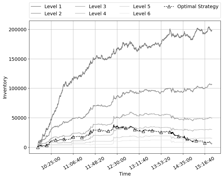
To the best of our knowledge, our work is unique in that it assesses the performance of the proposed market making strategy against LOB data. Specifically, we first use a rolling window approach to estimate the model parameters. We then test the calibrated model against actual LOB dynamics, allowing for adjustments of LO’s placements every second and determining the cash flows and inventory changes generated during the day. At day’s close, the HFM submits a MO to liquidate its final inventory, and determine the actual cost taking into account the state of the LOB. We find that the optimal placement yields, on average, larger revenue compared to the situation where $\pi(1,1)=0$ (such as in Adrian et al. 2020), even if $\pi(1,1)$ is estimated to be small and about $0.05$. Our empirical analysis lends strong support to demand stochasticity: the slope coefficient has a standard deviation which is about 200% larger than the average demand level, and a correlation of about 20% with the investors’ reservation price. Moreover, using real LOB data we estimate the optimal placement strategy based on a simple one-step ahead forecast to outperform the one that presumes a martingale price evolution.

The solution of the optimal control problem presents nontrivial mathematical challenges. While the first-order optimality conditions involves solving a quadratic equation, establishing the second-order conditions needed for the verification theorem is intricate. It involves establishing several clever estimates, in which we leverage direct inequalities implied by the primitives of our model.

The rest of the paper is organized as follows. In Section 2, we present the model setup together with our assumptions. Section 3 solves the Bellman equation for the control problem, and proves a verification theorem. In Section 4, we analyze in detail the main economic forces behind the optimal placement strategies. In Section 5, we measure the performance of our market making strategy against real LOB data. We delegate technical proofs to two appendices.

In this section we introduce our Limit Order Book (LOB) model and specify the type of considered strategies. We assume the market making strategy runs from time $0$ to a fixed time $T>0$. The HFM places bid and ask limit orders (LO) simultaneously on both sides of the LOB for a given asset at preset times $0=t_{0}<t_{1}<\dots<t_{N}<T$. Throughout, we set $t_{N+1}=T$ and $\mathcal{T}=\{t_{0},t_{1},\dots,t_{N+1}\}$. All variables introduced below are assumed to be defined on a probability space $(\Omega,\mathbb{P},\mathcal{F})$ equipped with a filtration $\{\mathcal{F}_{t}\}_{t\in\mathcal{T}}$, which represents the arrival of market makers’ available information through time.

Arrivals of buy and sell market orders (MO) are modeled by two Bernoulli processes. Specifically, let $\mathbbm{1}_{t_{k+1}}^{+}$ ($\mathbbm{1}_{t_{k+1}}^{-}$) be a Bernoulli random variable indicating whether there is at least one buy (sell) market order arriving during the time period $[t_{k},t_{k+1})$:

We assume that $\mathbbm{1}_{t_{k+1}}^{+},\mathbbm{1}_{t_{k+1}}^{-}\in$ $\mathcal{F}_{{t_{k+1}}}$ and

for $j^{\pm}\in\{0,1\}$, where $\pi_{{t_{k+1}}}:\{0,1\}\times\{0,1\}\to[0,1]$ is a deterministic probability distribution. The marginal conditional probabilities are denoted as

and throughout we assume that $\pi^{+}_{{t_{k+1}}}>0$ and $\pi^{-}_{{t_{k+1}}}>0$, for all $k=0,\dots,N$. Concretely, between two consecutive time steps $t_{k}$ and $t_{k+1}$, the arrival probability of at least one buy (sell) market order is ${\color[rgb]{0,0,0}\pi^{+}_{{t_{k+1}}}}$ (${\color[rgb]{0,0,0}\pi^{-}_{{t_{k+1}}}}$).

The ask (bid) LO is placed at time $t_{k}$, $k=0,\dots,N$, at the price level $a_{t_{k}}\in\mathcal{F}_{t_{k}}$ ($b_{t_{k}}\in\mathcal{F}_{t_{k}}$). We parameterize $a_{t_{k}}$ and $b_{t_{k}}$ as

where $L^{\pm}_{t_{k}}\in\mathcal{F}_{t_{k}}$ are the market maker’s spreads and $S_{t_{k}}\in\mathcal{F}_{t_{k}}$ is the fundamental price of the asset at time $t_{k}$. The assumptions on the fundamental prices process $\{S_{t_{k}}\}_{k=0,\dots,N+1}$ are further specified in Section 3.

The limit orders placed at time $t_{k}$ may be fully or partially executed during the time interval $[t_{k},t_{k+1})$, but only if there exists at least one arrival of a market order during that period. We assume that the number of filled shares on the bid side during the interval $[t_{k},t_{k+1})$ is given by

where $c_{t_{k+1}}^{-},p_{t_{k+1}}^{-}\in\mathcal{F}_{t_{k+1}}$ are positive random variables whose distribution is specified below in Assumption 1. When no sell market order arrives during the interval $[t_{k},t_{k+1})$, $\mathbbm{1}_{t_{k+1}}^{-}=0$ and the number of executions on the buy side is $0$. Here, $p_{t_{k+1}}^{-}$ is defined such that $S_{t_{k}}-p_{t_{k+1}}^{-}$ is the lowest price that all sell market orders arriving during $[t_{k},t_{k+1})$ can attain. In other words, bid limit orders placed by the HFM will not be executed during the interval $[t_{k},t_{k+1})$ if the price is smaller than $S_{t_{k}}-p^{-}_{t_{k}}$. We refer to $p_{t_{k+1}}^{-}$ as the reservation price for sellers. The demand slope $c_{t_{k+1}}^{-}$ measures the rate of increase in the number of filled shares of the bid order, as the order’s bid price $b_{t_{k}}$ gets closer to the fundamental price $S_{t_{k}}$. Symmetrically, the number of shares filled by the HFM’s ask limit order during $[t_{k},t_{k+1})$ is given by

The number of filled shares $Q^{\pm}_{{t_{k+1}}}$ is illustrated in Figure 1. The quantity $Q_{t_{k+1}}^{\pm}$ may be viewed as the “best” linear fit for the actual demand as shown in Figure 2. More details on the estimation of $Q^{\pm}_{{t_{k+1}}}$ are covered in the empirical analysis conducted in Section 5.

Next, we state our main assumptions on $c_{.}^{\pm}$ and $p_{.}^{\pm}$.

Next, we introduce some further notation related to $(c_{.}^{\pm},p_{.}^{\pm})$:

We consider the following maximization problem for the HFM:

where $\mathcal{A}$ is the collection of all $\mathcal{F}$-adapted processes, and $W_{T}$ and $I_{T}$ stand for the market maker’s cash holdings and inventory at the end of period $[0,T]$, respectively. The cash holding and inventory processes, $\{W_{t_{k}}\}$ and $\{I_{t_{k}}\}$, respectively, satisfy the following equations:

and

where $W_{t_{0}}=0$ and $I_{t_{0}}=0$.

The term $\lambda I^{2}_{T}\geq 0$ in the maximization problem (9) is the cost for holding inventory at the terminal time $T$. This formulation captures, in reduced form, the fact that HFMs tend to have de minimis balance sheets, thus making any overnight inventory costly to carry.⁴⁴ 4 Similar objective criteria have been proposed in earlier studies, such as Cartea & Jaimungal 2015 and Adrian et al. 2020. The penalty term for holding end-of-day inventory can also be interpreted as follows. We can rewrite the last two terms $S_{T}I_{T}-\lambda I_{T}^{2}$ in the above expectation as $(S_{T}-\lambda I_{T})I_{T}$. Then, $S_{T}-\lambda I_{T}$ is the average price per share that the HFM will get when liquidating her inventory $I_{T}$ via a MO, under the assumption of a linear instantaneous price impact. For instance, if $I_{T}>0$ ($I_{T}<0$), then the HFM will have to submit a sell (buy) MO, which will result in eating into the bid (ask) side of the book. We will validate the assumption of linear price impact in Section 5.

At time $t_{k}$, the value function of the control problem described above is given by

By the dynamic programming principle, we obtain it satisfies the following equation

We now proceed to find the optimal placement strategy for the market maker. Our objective is to derive it for a general adapted stochastic process of the fundamental price. To illustrate the procedure behind the construction, we first analyze the setting where the fundamental price process is a martingale, and obtain tractable formulas for the optimal bid and ask prices and the value function (see Subsection 3.1). In Subsection 3.2, we relax the martingale assumption and provide a general formula for general adapted stochastic price dynamics of the fundamental price.

References

• Adrian et al. (2020) Adrian, T., Capponi, A., Fleming, M., Vogt, E. & Zhang, H. (2020). Intraday market making with overnight inventory costs. Journal of Financial Markets 50, 100564.
• Amihud & Mendelson (1980) Amihud, Y. & Mendelson, H. (1980). Dealership market: Market-making with inventory. Journal of Financial Economics 8(1), 31–53.
• Bradfield (1979) Bradfield, J. (1979). A formal dynamic model of market making. Journal of Financial and Quantitative Analysis 14, 275–291.
• Cartea & Jaimungal (2015) Cartea, Á. & Jaimungal, S. (2015). Risk metrics and fine tuning of high-frequency trading strategies. Mathematical Finance 25(3), 576–611.
• Cartea et al. (2014) Cartea, A., Jaimungal, S. & Ricci, J. (2014). Buy low, sell high: A high frequency trading perspective. SIAM Journal on Financial Mathematics 5(1), 415–444.
• Cont et al. (2010) Cont, R., Stoikov, S. & Talreja, R. (2010). A stochastic model for order book dynamics. Operations Research 58(3), 549–563.
• Cvitanic & Kirilenko (2010) Cvitanic, J. & Kirilenko, A. A. (2010). High frequency traders and asset prices. Working paper. Preprint available at SSRN 1569067 .
• Gayduk & Nadtochiy (2018) Gayduk, R. & Nadtochiy, S. (2018). Liquidity effects of trading frequency. Mathematical Finance 28(3), 839–876.
• Glosten & Harris (1988) Glosten, L. R. & Harris, L. E. (1988). Estimating the components of the bid/ask spread. Journal of Financial Economics 21(1), 123–142.
• Guéant et al. (2013) Guéant, O., Lehalle, C.-A. & Fernandez-Tapia, J. (2013). Dealing with the inventory risk: a solution to the market making problem. Mathematics and Financial Economics 7(4), 477–507.
• Hall & LePage (1996) Hall, P. & LePage, R. (1996). On bootstrap estimation of the distribution of the studentized mean. Annals of the Institute of Statistical Mathematics 48(3), 403–421.
• Hasbrouck (1988) Hasbrouck, J. (1988). Trades, quotes, inventories, and information. Journal of Financial Economics 22, 229–252.
• Hendershott & Menkveld (2014) Hendershott, T. & Menkveld, A. J. (2014). Price pressures. Journal of Financial Economics 114(3), 405–423.
• Ho & Stoll (1981) Ho, T. & Stoll, H. R. (1981). Optimal dealer pricing under transactions and return uncertainty. Journal of Financial Economics 9(1), 47–73.
• Huang et al. (2012) Huang, K., Simchi-Levi, D. & Song, M. (2012). Optimal market-making with risk aversion. Operations Research 60(3), 541–565.
• Joint Staff Report (2015) Joint Staff Report (2015). The US treasury market on october 15, 2014. Tech. rep., Joint Staff Report, July.
• Kirilenko et al. (2017) Kirilenko, A., Kyle, A. S., Samadi, M. & Tuzun, T. (2017). The flash crash: High-frequency trading in an electronic market. The Journal of Finance 72(3), 967–998.
• Markets Committee et al. (2011) Markets Committee et al. (2011). High-frequency trading in the foreign exchange market. Bank For International Settlement .
• Menkveld (2013) Menkveld, A. (2013). High frequency trading and the new-market makers. Journal of Financial Markets 16, 712–740.
• Menkveld (2016) Menkveld, A. J. (2016). The economics of high-frequency trading: Taking stock. Annual Review of Financial Economics 8, 1–24.
• O’Hara & Oldfield (1986) O’Hara, M. & Oldfield, G. (1986). The microeconomics of market making. Journal of Financial and Quantitative Analysis 21(4), 2603–2619.
• Peng (2004) Peng, L. (2004). Empirical-likelihood-based confidence interval for the mean with a heavy-tailed distribution. The Annals of Statistics 32(3), 1192–1214.
• Securities and Exchange Commission (2010) Securities and Exchange Commission (2010). Concept release on equity market structure. Release No. 34-61358; File No. S7-02-10.