Optimal control of the decumulation of a retirement portfolio with variable spending and dynamic asset allocation
Abstract
We extend the Annually Recalculated Virtual Annuity (ARVA) spending rule for retirement savings decumulation (Waring and Siegel 2015) to include a cap and a floor on withdrawals. With a minimum withdrawal constraint, the ARVA strategy runs the risk of depleting the investment portfolio. We determine the dynamic asset allocation strategy which maximizes a weighted combination of expected total withdrawals (EW) and expected shortfall (ES), defined as the average of the worst five per cent of the outcomes of real terminal wealth. We compare the performance of our dynamic strategy to simpler alternatives which maintain constant asset allocation weights over time accompanied by either our same modified ARVA spending rule or withdrawals that are constant over time in real terms. Tests are carried out using both a parametric model of historical asset returns as well as bootstrap resampling of historical data. Consistent with previous literature that has used different measures of reward and risk than EW and ES, we find that allowing some variability in withdrawals leads to large improvements in efficiency. However, unlike the prior literature, we also demonstrate that further significant enhancements are possible through incorporating a dynamic asset allocation strategy rather than simply keeping asset allocation weights constant throughout retirement.
Keywords: Finance, risk management, optimal asset allocation, decumulation, defined contribution plan
JEL codes: G11, G22
AMS codes: 91G, 65N06, 65N12, 35Q93
Declarations of interest: None
Funding: Access to Wharton Research Data Services and historical
data from the Center for Research in Security Prices was provided through
an institutional subscription paid for by the University of Waterloo.
Peter Forsyth was also supported by the Natural Sciences
and Engineering Research Council of Canada (NSERC) under grant RGPIN-2017-03760.
1 Introduction
Defined Benefit (DB) pension plans are disappearing, being replaced by Defined Contribution (DC) plans. According to a recent study by the Organization for Economic Co-operation and Development (OECD), less than 50% of pension assets in 2018 were held in DB plans in over 80% of reporting jurisdictions. Moreover, in more than 75% of reporting countries the proportion of pension assets in DB plans was lower in 2018 relative to its level a decade earlier (OECD 2019). Note that the proportion of assets in DB plans is a lagging indicator of the shift to DC plans because employees who were historically covered by traditional DB plans have had more time to amass retirement savings. For example, in Israel the proportion of pension assets in DB plans dropped from 84% in 2008 to 56% in 2018. However, DB plans in that country were closed to new members in 1995 (OECD 2019). Almost 25 years later, over half of pension assets in Israel are still in DB plans.
The shift to DC plans is an inevitable consequence of corporations and governments being unwilling (or unable) to manage the risks associated with DB plans. In contrast, in DC plans the management of the financial assets is left up to individual investors. Given the long-term nature of retirement savings, this is a challenging task for most people. Assuming that investors do manage to accumulate healthy balances in their DC accounts, the situation gets even more complex upon retirement. Individuals must continue to manage their financial assets, and also determine a decumulation strategy to withdraw assets and fund spending with uncertain longevity. While it is often suggested that retirees should purchase annuities, this rarely happens in practice. For example, Milevsky and Young 2007 report findings from a survey of U.S. retirees indicating that only 8% of respondents who were DC plan members and less than 2% of all respondents chose to annuitize. More recently, it has been reported that only around 4% of retirees with DC plans at a prominent Canadian insurer opted to annuitize (Carrick 2020).
The reluctance of retirees to annuitize is sometimes called a puzzle, since standard life cycle economic models based on utility maximization suggest that annuitization is optimal (Peijnenburg et al. 2016). However, the overwhelming aversion to annuitization by retirees suggests that these economic models are missing something important. In practice, there are many reasons why retirees do not annuitize. MacDonald et al. 2013 list dozens of real-world factors including lack of true inflation protection, loss of control over capital, expensive pricing, the availability of other sources of guaranteed income such as government benefits, and paltry payments under some financial market conditions such as the current low interest rate environment.
Assuming that purchasing an annuity is undesirable, retirees must devise suitable decumulation strategies. A major component of these plans is how much money to withdraw over time. Retirees who withdraw fairly large sums run the risk of outliving their resources, i.e. the risk of “ruin”. On the other hand those who take out relatively small amounts may have less enjoyable retirements and leave their heirs with (unintended) large bequests.
Absent any annuitization, decumulation strategies can generally be classified as having fixed or variable withdrawals. Within these categories, several variations have been proposed. MacDonald et al. 2013 provide a nice summary of the various possibilities.11 1 MacDonald et al. 2013 also discuss hybrid strategies, which combine some level of annuitization with a (fixed or variable) decumulation scheme. We concentrate on strategies involving cash flows in the absence of any actual level of annuitization, so we ignore hybrid strategies in this work. In a fixed scheme, the amounts taken out each year are constant, typically in real (i.e. inflation-adjusted) terms. This results in a smooth profile of spending over time, assuming that the retiree remains solvent. In other words, the risk is effectively due to longevity: the danger is that there will not be sufficient funds to sustain a very long retirement period with fixed annual withdrawals. With a variable scheme, the amounts taken out fluctuate in response to factors such as investment returns. An extreme example of this would be a fixed percentage withdrawal strategy: the investor takes out a constant percentage of the portfolio value each year. In principle, this puts all of the risk onto the spending stream. It is impossible to run out of funds since something is always left for the next year. The obvious problem is that the amount withdrawn may fall below a minimally viable threshold if the retiree lives long enough. There are many other possibilities for variable schemes which attempt to strike a balance between the two fundamental risks of spending fluctuations and longevity, typically through changes in spending in response to financial market returns.
Perhaps the best known decumulation strategy is the 4% rule due to Bengen 1994. This fixed scheme states that retirees with an annually rebalanced portfolio split evenly between bonds and stocks can withdraw 4% of their initial wealth each year in real terms. Backtesting this rule on U.S. data showed that retirees would never have run out of funds, over any rolling historical 30-year period considered (Bengen 1994).
Backtesting using rolling historical periods is common in the practitioner literature. However, in general this approach seriously underestimates risk. Any two adjacent 30-year periods will have 29 years in common, any two 30-year periods beginning two years apart will have 28 years in common, etc. Consequently, the overall results will tend to be highly correlated, and this could be very misleading. The findings reported by Bengen 1994 address the question of what the historical experience would have been over a long period for someone who retired in a particular year and then followed the 4% rule. In other words, using rolling historical periods only considers what did happen, giving zero weight to any other plausible scenario that might have happened, and which could occur in the future. Two alternatives which can give a better sense of the risk involved are (i) to fit a parametric model to the historical data and then run a large number of Monte Carlo simulations, and (ii) to use block bootstrap resampling of the data (Politis and Romano 1994), which involves randomly drawing (with replacement) shorter periods of data and chaining them together over the decumulation horizon. We use both of these approaches below and find that the risk of using the 4% rule is quite significant.22 2 There are other reasons to think that Bengen 1994 understated the risk of the 4% rule. One is that data past 1992 was extrapolated using historical averages for financial market returns each year. For example, the 30-year performance of the rule given a retirement date of 1976 was assessed using 16 years of actual market data, followed by 14 years in which the returns for stocks and bonds and the inflation rate were constant each year at their long-term average values. This clearly understates the strategy’s risk for cases with several years in retirement after 1992. A more fundamental issue from today’s perspective is the reliability of the 4% rule during a lengthy period of very low interest rates. Finke et al. 2013 considered bond market conditions early in 2013 and estimated that the failure rate for the 4% rule assuming 10 years of below average bond returns and a 50% stock allocation was 32%, strongly suggesting that 4% is too high a withdrawal rate. Given that interest rates have continued to trend downwards more recently, there are solid grounds for pessimism about the viability of the 4% rule today.
As mentioned above, practitioners have proposed several variable schemes that allow spending to fluctuate in response to portfolio returns. These strategies typically permit higher initial withdrawal rates compared to fixed schemes such as the 4% rule. These enhanced withdrawal rates can be increased even further following portfolio gains, but need to be reduced (sometimes severely) after portfolio losses. Bengen 2001 considers fixed percentage withdrawals augmented with a floor and ceiling. The initial withdrawal rate can be increased in line with investment returns up to a maximum of 25% higher in real terms than the first withdrawal, or reduced no further than 10% below the real value of the initial withdrawal. Bengen 2001 concludes that this strategy permits a safe initial withdrawal rate of about 4.6%, notably higher than the fixed 4% rule. Guyton and Klinger 2006 explore the use of a complicated set of heuristic rules governing withdrawals, portfolio decisions, caps and freezes on inflation adjustments, etc. They conclude that an initial withdrawal rate of 5.2%-5.6% is sustainable given a portfolio equity allocation of 65%. As a third example, Waring and Siegel 2015 introduce the Annually Recalculated Virtual Annuity (ARVA) rule, which is based on the idea that the amount taken out of the portfolio in any given year should be based on the annual cash flow from a virtual (i.e. imaginary) fixed term annuity that could be purchased using the current value of the portfolio. This strategy is similar to a fixed percentage withdrawal scheme in that the portfolio can never be fully depleted, but withdrawals can become unsustainable small if retirement is sufficiently long and/or portfolio returns are poor. Alternatively, the ARVA rule will lead to increased withdrawals following good investment returns.
Pfau 2015 compares the performance of several spending strategies by Monte Carlo simulation with parameters calibrated to long term (1890-2013) annual data for financial market returns and inflation. Pfau 2015 begins with a modification of the Bengen 1994 rule which uses constant inflation-adjusted withdrawals, but with a spending rate of 2.86% rather than 4%. This lower rate of 2.86% was estimated on the basis of there being at least a 90% chance of 1.5% of the initial amount of real wealth remaining after 30 years of withdrawals, assuming a 50/50 portfolio allocation between stocks and bonds. Using the same portfolio allocation and the same 90% criterion for other strategies permitted higher initial spending rates. For example, the initial spending rate for Bengen 2001’s fixed percentage scheme with a floor of 85% of the real value of the first year’s withdrawal and a corresponding ceiling of 120% resulted in a sustainable initial spending rate of 3.31%. As additional examples, Pfau 2015’s implementations of the ARVA approach (Waring and Siegel 2015) and the Guyton and Klinger 2006 rules produced sustainable initial spending rates of 4.34% and 4.82% respectively.
An important issue that has not been investigated much in the practitioner literature on decumulation is the effect of a more sophisticated approach to asset allocation, beyond simply rebalancing to a constant weighting of bonds and stocks. Tretiakova and Yamada 2017 explore the performance of rebalancing to maintain a constant level of a (time-varying) equity market risk measure using several withdrawal rules and report that sustainable spending is significantly improved. However, this leaves open the question of the impact of using an asset allocation strategy that is optimized to achieve a well-defined financial objective. Implementing such an approach necessitates specifying a suitable objective function and solving the resulting optimization problem, which in turn requires more technically sophisticated methods.
Along these lines, Dang et al. 2017 suggest using a multi-period mean variance objective function to examine the effect of different (fixed) withdrawal rates coupled with an adaptive portfolio allocation strategy. The objective function is posed in terms of the mean and variance of the final wealth at time . Dang et al. 2017 assume that most 65-year olds can expect to live for 20 years with high probability, and thus set a wealth target of one-half of the initial wealth at years (after retirement). The idea is that retirees can decide how to hedge longevity risk at age , expecting to have spent one-half of their original wealth up to then.
Irlam 2014 uses dynamic programming methods to determine asset allocation, given an objective of maximizing the number of years of solvency divided by the number of years lived. This is the only study we are aware of in the practitioner literature for which the asset allocation depends on a specified financial objective. Irlam 2014 concludes that asset allocation rules that depend only on time such as “age in bonds” or various target-date fund glide paths require a higher amount of investment in order to obtain the same withdrawal rates in retirement, as compared to his approach where the asset allocation is time and state-dependent. However, Irlam 2014 only considers a fixed annual withdrawal amount in retirement.
In this work we further explore the effect of a variable spending rule in combination with an asset allocation strategy tailored to optimizing a financial objective. In particular, we use an ARVA spending rule augmented by constraints on minimum and maximum annual withdrawals. The minimum withdrawal constraint means that there is risk of depleting the portfolio entirely prior to the end of the investment horizon. We use the Expected Shortfall (ES) of the terminal portfolio value as a measure of risk. The ES at level is the mean of the worst of outcomes, and is thus a measure of tail risk. As a measure of reward, we use total Expected Withdrawals (EW). Based on a parametric model calibrated to historical market data, we determine the portfolio allocation strategy that optimizes the multi-objective Expected Withdrawals-Expected Shortfall (EW-ES) objective function.33 3 Forsyth et al. 2020 use the same measure of reward, but minimize the downside variability of withdrawals for an ARVA type spending rule, i.e. the risk measure is downward withdrawal variability. There are some other noteworthy differences between this work and that of Forsyth et al. 2020. First, we impose upper and lower bounds on annual withdrawals. Second, the assumed underlying financial model is more complex here, as it incorporates stochastic bond market returns.
A similar measure of risk and reward for DC plan decumulation is used in Forsyth 2020c. However, Forsyth 2020c uses the withdrawal amount as a control, rather than an ARVA spending rule. In this case, Forsyth 2020c shows that the withdrawal control is essentially a bang-bang type control, with minimum withdrawals during the earlier years of retirement. Use of the ARVA spending rule (with constraints) provides more control over the timing of withdrawals.
We verify the robustness of this strategy through tests using bootstrap resampling of historical return data. Our tests show that the ARVA spending rule coupled with an optimal allocation strategy is always more efficient than a constant withdrawal, constant weight strategy. In fact, our optimal dynamic ARVA strategy outperforms this alternative even when the minimum withdrawal under ARVA is equal to the constant withdrawal with constant weights. This verifies that allowing some variability in withdrawals sharply reduces the risk of depleted savings, consistent with Pfau 2015 and Tretiakova and Yamada 2017. In addition, we demonstrate that solving an optimal stochastic control problem to specify the asset allocation can provide further significant benefits beyond those obtained by permitting withdrawal variability alone.
2 ARVA Spending Rule
Consider the following spending rule. Each year, a virtual (hypothetical) fixed term annuity is constructed, based on the current portfolio value, the number of remaining years of required cash flows, and a real (inflation adjusted) interest rate. The investor then withdraws an amount based on the hypothetical payment of this virtual annuity. Clearly, the annual payments will be variable, since the virtual annuity is recalculated each year, and is a function of the current portfolio value. The portfolio is liquidated at the end of the investment horizon. A surplus will be returned to the investor (or the investor’s estate). Any shortfall must be settled at this time as well.
We are now faced with the choice of determining a timespan for the virtual fixed term annuity. Rather than specifying a maximum possible lifespan (which would be overly conservative), we assume that retirees are in the top 20% of the population in terms of conditional expected longevity (Westmacott 2017). Consider a retiree who is years old at . Assuming that the year old retiree is alive at time , let be the time at which 80% of the cohort of year olds are expected to have passed away, conditional on all members of the cohort being alive at time . At time , the fixed term of the virtual annuity is then . This mortality assumption has the effect of providing increased spending during the early years of retirement. By varying the fraction of the cohort assumed to have passed away, we can increase/decrease spending in early retirement years at the cost of decreased/increased spending in later years. Note that our ARVA withdrawal amount is not generally the same as would be obtained from a currently purchased life annuity.
Given the real interest rate , the present value of an annuity which pays continuously at a rate of one unit per year for years is denoted by the annuity factor
| (2.1) |
It follows that is the continuous real annuity payment for years, which can be purchased with wealth at time . We make the assumption that withdrawals occur at discrete times in
| (2.2) |
where denotes the time that the year old retiree begins to withdraw money from the DC plan. We assume the times in are equally spaced with , . We let one year. We determine the cash withdrawal at time by converting the continuous payment above into a lump sum received in advance of the interval . This lump sum withdrawal at is , where
| (2.3) |
In this work, we will compute equation (2.3) based on the CPM 2014 mortality tables (male) from the Canadian Institute of Actuaries44 4 www.cia-ica.ca/docs/default-source/2014/214013e.pdf to compute with . Further discussion of the ARVA spending rule can be found in Forsyth et al. 2020.
3 Investment Market
We assume that the investment portfolio consists of two index funds. These funds include a stock market index fund and a constant maturity bond index fund. Let the investment horizon be , and and respectively denote the real (inflation adjusted) amounts invested in the stock index and the bond index. These amounts can change due to (i) changes in the real unit prices and (ii) the investor’s asset allocation strategy. In the absence of the application of an investor’s control, all changes in and result from changes in asset prices.
We model the stock index (in the absence of an applied control) as following a jump diffusion process. Let , i.e. is the instant of time before , and let be a random jump multiplier. When a jump occurs, . Use of jump processes allows for modelling of fat-tailed (non-normal) asset returns.55 5 Appendix A documents evidence of leptokurtic behavior for both of the indexes that we use in our tests. We assume that follows a double exponential distribution (Kou and Wang 2004). The probability of an upward jump is , with being the probability of a downward jump. The density function for is
| (3.1) |
Define
| (3.2) |
Without an applied control,
| (3.3) |
where is the (uncompensated) drift rate, is the diffusive volatility, is a Brownian motion, is a Poisson process with intensity parameter , and are i.i.d. positive random variables having distribution (3.1). Moreover, , , and are assumed to all be mutually independent.
As in MacMinn et al. 2014 and Lin et al. 2015, we use a common practitioner approach and model the returns of the constant maturity bond index (absent an applied control) as a stochastic process. This approach has the advantage that estimating model parameters from market data is quite straightforward, without the need to devise a parametric process for real interest rates. As in MacMinn et al. 2014, we assume that the constant maturity bond index follows a jump diffusion process. In particular, . In the absence of control, evolves as
| (3.4) |
where the terms in equation (3.4) are defined analogously to equation (3.3). In particular, is a Poisson process with positive intensity parameter , and has distribution
| (3.5) |
and . , , and are assumed to all be mutually independent. The term in equation (3.4) represents an additional cost of borrowing (), i.e. a spread between borrowing and lending rates. We assume that the diffusive components of and are correlated, i.e. . However, the jump process terms for these two indexes are assumed to be mutually independent.66 6 See Forsyth 2020b for a discussion of the evidence for stock and bond price jump independence.
It is possible to include more complex stock and bond processes, such as stochastic volatility for example. However, Ma and Forsyth 2016 have shown that including stochastic volatility effects does not have a significant effect on the results for long term investors. In order to verify the robustness of the strategies, we will determine the optimal controls using the parametric model based on equations (3.3) and (3.4). We then test these controls on bootstrapped resampled historical data. This is quite a strict test, since the bootstrapped resampling algorithm makes no assumptions about the underlying bond and stock stochastic processes.
We define the investor’s total wealth at time as . We impose the constraints that (assuming solvency) shorting stock and using leverage (i.e. borrowing) are not allowed. Insolvency can arise from withdrawals. If this happens, the portfolio is liquidated and debt accumulates at the borrowing rate. The borrowing rate is taken to be the return on the constant maturity bond index plus a spread .
4 Notational Conventions
For ease of explanation, we will occasionally use the notation and . Earlier in equation (2.2) we specified a set of times for which withdrawals are permitted. We now expand the scope of so that portfolio rebalances are also allowed at those times, i.e. is the set of withdrawal/rebalancing times. More specifically, let the inception time of the investment be . At each withdrawal/rebalancing time , , the investor (i) withdraws an amount of cash from the portfolio, and then (ii) rebalances the portfolio. At , the portfolio is liquidated and the final cash flow occurs.
Given a time dependent function , we use the shorthand notation and . We assume that no taxes are triggered by rebalancing. This would normally be the case in a tax-advantaged DC savings account. Since we assume yearly application of the controls (rebalancing), we expect transaction costs to be small and hence they can be safely ignored.77 7 It is possible to include transaction costs, but this will increase computational cost (Van Staden et al. 2018). With no taxes or transaction costs, it follows that .
The multi-dimensional controlled underlying process is denoted by , with . The realized state of the system is . Let the rebalancing control be the fraction invested in the stock index at rebalancing date , i.e.
| (4.1) |
The controls depend on the state of the investment portfolio before the rebalancing occurs, i.e. , . We search for the optimal strategies amongst all controls with constant wealth after cash withdrawal,
| (4.2) |
We assume that rebalancing occurs instantaneously, with the implication that the probability of a jump occurring in either index is zero during the rebalancing period .
Let represent the set of admissible values of the control . An admissible control , where is the admissible control set, can be written as . We impose no-shorting and no-leverage constraints by specifying
| (4.3) |
We also apply the constraint that if , the stock index holding is liquidated,
| (4.4) |
and no further stock purchases are permitted, with the result that debt accumulates at the bond return plus a spread. In addition, we define as the tail of the set of controls in , i.e. .
5 Risk and Reward Measures
Initially, we describe our measure of risk. Suppose is the probability density function of terminal wealth at , and let
| (5.1) |
so that Prob. We can interpret as the Value at Risk (VAR) at level . The Expected Shortfall (ES) at level is then
| (5.2) |
which is the mean of the worst fraction of outcomes. Usually, . We emphasize that the definition of ES in equation (5.2) uses the probability density of the final wealth distribution, not the density of loss. This has the implication that a larger value of ES is desirable (the worst case average portfolio value at ).88 8 The negative of ES is often called Conditional Value at Risk (CVAR), which has been used as a risk measure in several prior asset allocation studies (Gao et al. 2016; Cui et al. 2019; Forsyth 2020a, e.g.).
Define . Given an expectation under control , , Rockafellar and Uryasev 2000 show that can be alternatively written as
| (5.3) |
The notation indicates that is as seen at . This definition is then the pre-commitment ES. A strategy based on optimizing the pre-commitment ES at time zero is time inconsistent, since the investor may have an incentive to deviate from the strategy at . Thus, some authors have described pre-commitment strategies as being non-implementable. However, this is really a matter of interpretation: we consider the pre-commitment strategy as a useful technique to compute an appropriate value of in equation (5.3). In fact, the strategy which fixes , is the induced time consistent strategy (Strub et al. 2019), and is consequently implementable. We delay further discussion of this point to Section 6.
Our measure of reward is expected total withdrawals (EW), defined as
| (5.4) |
Note that we do not discount withdrawals, with either a market-based measure of the appropriate risk-adjusted discount rate or with a subjective discount rate. This reflects a desire to avoid basing our strategy on parameters that are difficult to estimate. Since the portfolio weights will depend on realized investment returns and withdrawals over time, it is problematic to estimate the appropriate risk-adjusted discount rate. Moreover, it is likely to be difficult to determine a subjective discount rate, which could easily vary across investors and/or over time. However, we observe that the economic effect of discounting the withdrawals would be to make earlier withdrawals more desirable. We have already incorporated a similar effect through the mortality boost to the spending rule discussed in Section 2 above.
6 Objective Function
Our overall approach involves a statistical tradeoff between reward and risk, similar to mean-variance portfolio analysis but with different measures of reward and risk. The main alternative would be a standard life cycle approach, where we would maximize a specified utility function. This would raise concerns related to estimating parameters such as risk aversion or elasticities of intertemporal substitution, similar to the subjective discount rate discussed in the preceding paragraph. However, this would pose more of a problem since the appropriate form of the utility function itself is open to question. The most popular specification in the literature is power utility, which implies constant relative risk aversion. However, a recent empirical study by Meeuwis 2020 of the portfolio holdings and income of millions of US retirement investors indicates that such a model is mis-specified: actual investors exhibit decreasing (not constant) relative risk aversion. More generally, the standard life cycle approach in principle requires knowledge of the investor’s total wealth including wealth due to human capital, illiquid assets such as a home, etc., not just a retirement savings portfolio. Although the standard life cycle approach offers some insightful theoretical implications, it is difficult to use in practice because the information required is often either not available or measured very imprecisely. We can also point out that the empirical validity of the standard life cycle approach has been questioned on behavioral grounds (Thaler 1990). Accordingly, we avoid standard life cycle modelling based on utility functions. We also avoid extending the standard life cycle approach to more complicated preference specifications which may fit the data better (see, e.g. Meeuwis 2020, and references therein). Instead, we take the relatively simpler approach of optimizing the reward-risk tradeoff.
Expected withdrawals (EW) and expected shortfall (ES) are conflicting measures, so we use a scalarization technique to find the Pareto points for this multi-objective optimization problem. Informally, for a given scalarization parameter , we seek the control that maximizes
| (6.1) |
More precisely, we define the pre-commitment EW-ES problem in terms of the value function
| (6.2) |
and the constraints
| (6.3) |
By reversing the order of the in equation (6.2), the value function can be written as
| (6.4) |
Denote the investor’s initial wealth at by . Observe that the inner supremum in equation (6.4) is a continuous function of . Then, assuming that the domain of is compact, we define
| (6.5) |
Regarding as fixed , the following proposition follows immediately:
Proposition 6.1 (Pre-commitment strategy equivalence to a time consistent policy for an alternative objective function).
The pre-commitment EW-ES strategy determined by solving with from equation (6.5) is the time consistent strategy for an equivalent problem with fixed and value function defined by
| (6.6) |
Remark 6.1 (EW-ES induced time consistent strategy: an implementable control).
In the following, we consider the actual strategy followed by the investor for any as given by the induced time consistent strategy99 9 See Strub et al. 2019 for a discussion of induced time consistent strategies. that solves problem (6.6) with the fixed value of from equation (6.5). This strategy is identical to the EW-ES strategy at time zero. Hence, we refer to this strategy as the EW-ES strategy. It is understood that this refers to the strategy that solves the time consistent equivalent problem (6.6) for any . Consequently, this strategy is implementable (Forsyth 2020a) (the investor has no incentive to deviate from this control for ).
7 Solution Method
To solve the pre-commitment EW-ES problem (6.2), we start by interchanging the to arrive at equation (6.4). We expand the state space to , and define the auxiliary value function
| (7.1) |
and slightly revised constraints
| (7.2) |
We can solve auxiliary problem (7.1) using dynamic programming. The optimal control at time is determined from
| (7.3) |
Following the dynamic programming algorithm, we move the solution backwards across across time via
| (7.4) |
where , and . is based on our ARVA spending rule (see Section 9 for a precise specification). Note that the spending rule will be a function of wealth before withdrawal. At , we have
| (7.5) |
For times , there are no cash flows or controls applied. Recall that all quantities are real, and that there is no discounting. The iterated expectation property combined with Itô’s Lemma for jump processes in equations (3.3-3.4) then gives
| (7.6) |
Define
| (7.7) |
It is then straightforward to see that formulation (7.1-7.6) is equivalent to problem (6.2).1010 10 See Forsyth 2020a for discussion of a similar problem.
We briefly describe our numerical solution approach. We refer the reader to Forsyth and Labahn 2019 and Forsyth 2020b for further details. We start by solving the auxiliary problem (7.1-7.2) with fixed values of , and . Since shorting of the stock index is not allowed, . We localize the domain on a finite localized domain . The computational domain for is discretized using equally spaced nodes in the direction. Similarly, we define the localized domain for to be . The computational domain for is discretized using equally spaced nodes in the direction. Since the investor can become insolvent due to withdrawals, we also define a mirror image grid for (Forsyth 2020b).
We use the Fourier methods described in Forsyth and Labahn 2019 to solve PIDE (7.6) between rebalancing times. Wrap-around errors are minimized using the domain extension technique in Forsyth and Labahn 2019. The localized domain , with (units for are thousands of dollars). Numerical tests showed that the errors involved in this domain localization were at most in the fifth digit.
At rebalancing times, we discretize the equity fraction using equally spaced nodes and evaluate the right hand side of equation (7.3) using linear interpolation. We then solve the optimization problem (7.3) using exhaustive search over the discretized values.
Given an approximate solution of the auxiliary problem (7.1-7.2) at , which we denote by , we then compute the solution of problem (6.2) using equation (7.7). More specifically, we solve
| (7.8) |
given initial wealth . We solve this outer optimization problem using a one-dimensional optimization algorithm.1111 11 Since the problem is not guaranteed to be convex, we cannot be sure that we converge to the global maximum. Additional testing based on a search over the finest grid suggests that we do indeed have the globally optimal solution.
If and , then Prob. In addition, for large values of the withdrawal is capped at . As a result the objective function is almost independent of the control, and thus determination of the control becomes ill-posed. To avoid this, we change the objective function (6.2) by adding a stabilizing term , giving
| (7.9) |
A negative value for forces the strategy to invest in the bond index when is very large and , where the original control problem is ill-posed. This choice is consistent with de-risking retirement assets as soon as possible (Merton 2014). Setting gave the same results as setting to four digits for the summary statistics of the problem solution. This is due to the fact that outcomes with very large terminal wealth are highly unlikely.
8 Data and Parameter Estimates
As mentioned above, our model assumes that the retiree’s portfolio is allocated to either a stock index or a constant maturity bond index. In order to have a long history encompassing expansions, recessions, stock market booms and crashes, and different levels of interest rates, we use US financial market data. In particular, the stock index is taken to be the Center for Research in Security Prices (CRSP) Value-Weighted Index1212 12 This is a total return index of the broad US stock market, reflecting both distributions such as dividends and capital gains/losses due to price changes., while the bond index is the CRSP 30-Day Treasury bill (T-bill) Index. Both indexes are measured on a monthly basis from January 1926 through December 2018, giving a total of 1,116 observations. To work in real terms, we deflate both indexes by the Consumer Price Index (CPI), which was also provided by CRSP.1313 13 The CRSP data used in this study was obtained through Wharton Research Data Services (WRDS). This service and the data available thereon constitute valuable intellectual property and trade secrets of WRDS and/or its third party suppliers.
We use the threshold technique (Mancini 2009; Cont and Mancini 2011; Dang and Forsyth 2016) to estimate the parameters for the stochastic process models (3.3-3.4) (see Appendix A). All estimated parameters reflect real (inflation adjusted) returns. Table 8.1 shows the annualized parameter estimates. For reference, the table also gives the estimated parameters for the two time series assuming geometric Brownian motion (GBM).1414 14 The GBM parameter estimates are calculated using maximum likelihood estimation. For the threshold case, after removing any returns which occur at times corresponding to jumps in either series, the correlation is then estimated using the remaining sample covariance.
The annualized real value-weighted stock index parameters in Table 8.1 for the double exponential jump diffusion model correspond to an (uncompensated) drift rate of 8.6% and a diffusive volatility of 14.6%. Jumps in the stock index are estimated to occur about once every three years. Conditional on a jump occurring, a downwards jump is about 3 times more likely than an upwards jump. The mean jump size is about 23% in the upward direction and 18% in the downward direction. Since the standard deviation is equal to the mean for an exponentially distributed random variable, the magnitudes of both upward and downward jumps can vary considerably. The corresponding GBM parameter estimates imply a drift of about 8% per annum, with a volatility of 18.5%. This volatility is higher than the diffusive volatility for the jump model since in the GBM case this term effectively combines the effects of volatility due to both diffusion and jumps.
Turning to the T-bill index, the annualized jump model parameters correspond to a real (uncompensated) drift of approximately 0.45% and a diffusive volatility of about 1.3%. Jumps are estimated to occur about every 2 years, slightly more often than for the stock index. Downward jumps are again more likely than upward jumps, though somewhat less so compared to the stock index. The mean jump size is around 1.5% in the upward direction, and about 1.7% in the downward direction. The GBM parameter estimates indicate a drift that is also about 0.45%, and a volatility of approximately 1.8%. Finally, the correlation between the diffusive terms for the two indexes is quite low, around .083 for the jump model and .059 for the GBM case.
| Real CRSP Value-Weighted Stock Index | |||||||
| Method | |||||||
| Threshold () | .08607 | .14600 | .32258 | .23333 | 4.3578 | 5.5089 | .08311 |
| GBM | .08044 | .18460 | N/A | N/A | N/A | N/A | .05870 |
| Real 30 Day T-bill Index | |||||||
| Method | |||||||
| Threshold () | .00454 | .01301 | .51610 | 0.39580 | 65.875 | 57.737 | .08311 |
| GBM | .00448 | .01814 | N/A | N/A | N/A | N/A | .05870 |
9 Investment Scenario
In order to focus exclusively on decumulation, we consider an investor just entering retirement at age 65 with savings of $1 million. Our investor is assumed to have the life expectancy characteristics of a Canadian male. According to the CPM 2014 mortality table, this investor has a 13% probability of attaining the age of 95 and a 2% probability of reaching the century mark. We set the investment horizon to be 30 years.
We alter the standard ARVA spending rule so as to include an annual floor of and an annual cap of . Recall that all quantities are expressed in real (i.e. inflation-adjusted) terms. Our modified ARVA spending rule is then
| (9.1) |
where is given in equation (2.3). To provide more context, a Canadian male who has worked for 40 years in a high-earning occupation can expect to receive slightly over $20,000 per year in government benefits. Hence, we are assuming that the minimum total amount needed per year is about per year. Of course, the investor would like to withdraw more than the minimum amount of $30,000. However, as noted we also place a cap of $80,000 per year on withdrawals. The cap prevents the retiree from reducing savings very quickly, establishing a buffer against potential poor investment returns. We are thus effectively assuming that our retiree has no need for income above per year.1515 15 It is also worth noting that Canadian government benefits are reduced when total income exceeds about $80,000 per year, providing further incentive to not withdraw more than the specified cap.
Our retired investor withdraws cash and rebalances his portfolio at the start of each year, beginning immediately. The interest rate used in the ARVA calculation (2.3) is set equal to the estimated value of , which is given in Table 8.1 as 0.454%. Table 9.1 summarizes the base case investment scenario. Note that monetary units here and in the following tables and plots are expressed in thousands of (real) dollars.
| Investment horizon (years) | 30 |
|---|---|
| Investor () | 65-year old Canadian male |
| Mortality table | CPM 2014 |
| Equity market index | CRSP value-weighted index (real) |
| Bond index | 30-day T-bill index (real) |
| Initial portfolio value | 1,000 |
| Cash withdrawal/portfolio rebalance times (years) | |
| 80 | |
| 30 | |
| Borrowing spread when | |
| Interest rate for ARVA computation (2.3) | |
| Rebalancing interval (years) | 1 |
| Market parameters | See Table 8.1 |
Since the investor uses a risky portfolio to fund minimum cash flows annually, there is clearly no guarantee that he will not run out of savings if he has survived to age 95. As outlined above, we seek an investment strategy that minimizes risk as measured by expected shortfall (ES), as defined by equation (5.2). We use , so we are trying to minimize the adverse consequences measured by the average outcome in the worst 5% of the distribution. As indicated in Table 9.1, when we assume that debt accumulates at the rate given by the current return on 30-day T-bills plus a spread of .
We focus solely on measured outcomes for the investment account, but it is easy to imagine that our retiree also owns real estate such as a home. In this case, the ES risk could be hedged using a reverse mortgage with the home as collateral. However, we assume that the investor wants to avoid using a reverse mortgage if at all possible, so we seek an investment strategy that minimizes the magnitude of ES risk on its own. Our scenario shares some features with the behavioural life cycle approach originally described in Shefrin and Thaler 1988. In this framework, investors divide their wealth into separate “mental accounts” containing funds intended for different purposes such as current spending or future needs. The standard life cycle approach assumes that wealth is completely fungible across any such accounts, so that the same increase in wealth from any source (e.g. positive returns for a financial market portfolio, an increase in the value of one’s house, lottery winnings, etc.) has the same effect on consumption. In contrast, in the behavioral approach wealth is not completely fungible, so the effects of increased wealth depend on the source of the increase. In our case, even if the investor’s wealth rises because the value of his real estate has increased, there will be no impact on the amount withdrawn from the retirement portfolio. The real estate account will only be accessed as a last resort. It is assumed to be there in the background if needed, but it is ignored in our analysis.
10 Numerical Results: Synthetic Market
We evaluate the performance of three alternative strategies based on the scenario described by Table 9.1: (i) constant withdrawals and investment portfolio rebalanced to maintain constant asset allocation weights (in particular, we set instead of the values given in Table 9.1 so that this strategy corresponds to the 4% rule of Bengen 1994); (ii) ARVA withdrawals as indicated in Table 9.1 and investment portfolio rebalanced to maintain constant asset allocation weights; and (iii) ARVA withdrawals as indicated in Table 9.1 and investment portfolio rebalanced to optimal asset allocation weights, in accordance with solving the pre-commitment EW-ES problem (6.2) by the methods described in Section 7. In each case, the performance evaluation is based on Monte Carlo simulated paths of market returns based on the parametric model (3.3-3.4), with statistics of interest calculated across all paths. We refer to this as a synthetic market, since the data used is generated by simulation of the parametric model rather than taken directly from actual historical market returns.1616 16 We provide results based on historical market returns below in Section 11 and Appendix B.
We begin with the first strategy described above: constant withdrawals based on the 4% rule () and constant weights, i.e. in equation (6.3). The results for the equity index weight are shown in Table 10.1. This table also displays the results for , since this is approximately the equity weight which results in the maximum ES. We conjecture that this low equity weight is due to our use of ES to measure risk, compared to the more typical standard deviation. As increases past 0.15, the magnitude of ES increases strongly. Taking on more equity market risk results obviously leads to higher ES. Of course reward also rises, as shown by the median value of terminal wealth .1717 17 In general, our measure of reward is total expected withdrawals. However, in this case the withdrawals are fixed, so wealth is drawn down slowly given a sufficiently high and decent equity market returns, resulting in relatively high values for .
| Equity Weight | ES () | Median[] |
|---|---|---|
| 0.00 | ||
| 0.10 | ||
| 0.15 | ||
| 0.20 | ||
| 0.30 | ||
| 0.40 | ||
| 0.50 | ||
| 0.60 | ||
| 0.70 | ||
| 0.80 | ||
| 0.90 | ||
| 1.00 |
To see the benefit of the ARVA withdrawal strategy, we repeat the Monte Carlo simulations from above, except that here the ARVA spending strategy (2.3) is used with the constraints and . The results are shown in Table 10.2, which has an additional column compared to Table 10.1. This extra column shows the expected average withdrawals over the decumulation period, .1818 18 This column was excluded from Table 10.1 because in that case the annual withdrawals were constant at 40. In Table 10.2 the largest ES is for . This equity weight gives an expected annual withdrawal of . Recall that the largest ES from Table 10.1 was , with constant annual withdrawals of 40. There is a dramatic improvement in ES, despite higher average withdrawals. As another observation, in Table 10.2 the strategy with has better ES than the best result in Table 10.1, while the average expected withdrawal is , again compared to the constant withdrawal of . Overall, our comparison between strategies with constant asset weights and constant vs. variable spending (the ARVA rule augmented with a floor and a cap) is consistent with the results in studies such as Pfau 2015, albeit with different measures of risk and reward: a variable spending rule allows for both higher average withdrawals and lower risk as measured by ES.
| Equity Weight | ES () | Median[] | |
|---|---|---|---|
| 0.0 | |||
| 0.1 | |||
| 0.2 | |||
| 0.3 | |||
| 0.4 | |||
| 0.5 | |||
| 0.6 | |||
| 0.7 | |||
| 0.8 | |||
| 0.9 | |||
| 1.0 |
We next consider our third strategy of ARVA withdrawals with optimal asset allocation. In particular, we consider the scenario described in Table 9.1 and solve for the optimal control for the pre-commitment EW-ES problem given by equation (6.2) using the methods discussed in Section 7. We store the optimal control and then carry out Monte Carlo simulations to calculate statistical properties as above but with applying along each path rather than rebalancing to constant weights. We reiterate that for all times , this corresponds to the induced time consistent strategy that solves equation (6.6).
Before presenting the main results, we first verify the convergence of the algorithm given in Section 7 that is used to solve the optimal control problem given by equation (6.2). Table 10.3 shows a test with various levels of grid refinement for a fixed value of in equation (6.2). At each grid refinement, we compute and store the optimal controls which are then used in Monte Carlo simulations. The algorithm in Section 7 and the Monte Carlo simulations are in good agreement. As expected, the value function appears to be converging at almost a quadratic rate. The other quantities ES and expected average withdrawals which are derived from the algorithm in Section 7 converge a bit more erratically. Results reported below for all cases with optimal asset allocation are calculated using the finest grid from Table 10.3.
| Algorithm in Section 7 | Monte Carlo | ||||
|---|---|---|---|---|---|
| Value | |||||
| Grid | ES () | Function | ES () | ||
Table 10.4 shows the results for the ARVA spending rule with optimal asset allocation from solving the pre-commitment EW-ES problem (6.2) for various values of . In addition to ES, expected average withdrawals , and median , Table 10.4 shows the average throughout the investment horizon of the median value of the fraction of the portfolio invested in equities in the furthest right column. This gives a rough indication of the equity market risk taken on over the period. As indicated by equation (6.1), increasing places more emphasis on risk relative to reward. As a result, the optimal equity allocation tends to decrease with . This is also reflected in reduced median and expected average withdrawals. The benefit from higher is a lower magnitude of ES. Consider the case here with which results in ES of , expected average withdrawals of 52.35, and median of 129.97. This strategy has an average median equity allocation of 0.34. Contrast this with the result reported in Table 10.2 for , which had about the same ES (), but expected average withdrawals of just 42.07 and median terminal wealth of 64.31. In this case, using an optimal asset allocation strategy compared to a constant weight strategy results in about the same ES but significantly higher average withdrawals and about twice as much median . This attests to the benefits of optimizing the asset allocation strategy, in addition to allowing for variable withdrawals.
| ES () | Median[] | |||
|---|---|---|---|---|
| 0.1 | ||||
| 0.3 | ||||
| 0.5 | ||||
| 1.0 | ||||
| 1.75 | ||||
| 2.5 | ||||
| 5.0 | ||||
| 10.0 | ||||
| 20.0 | ||||
| 100.0 | ||||
| 1000.0 |
To further investigate the benefits of using an optimal asset allocation strategy, we plot the efficient frontiers of expected average withdrawals vs. ES in Figure 1(a). We show these frontiers for (i) the ARVA spending rule with optimal asset allocation as computed by solving the pre-commitment EW-ES problem (6.2), with results provided in Table 10.4; (ii) the ARVA spending rule with a constant weight asset allocation strategy, with results shown in Table 10.2; and (iii) a constant withdrawal of with a constant weight strategy, with just the best result (i.e. highest ES) from Table 10.1.1919 19 This last case leads to just a single point in our plot since withdrawals are fixed at 40 regardless of the asset allocation and all other constant equity weights lead to lower ES. Note that we have removed all non-Pareto points from these frontiers for plotting purposes. Figure 1(a) shows that even with constant asset allocation weights the ARVA spending rule is much more efficient than a constant withdrawal strategy which also has constant asset allocation weights. In fact, ARVA alone provides about 50% higher expected average withdrawals for the same ES achieved by a constant withdrawal strategy by allowing for a higher stock allocation and limited income variability. The case with optimal asset allocation with the ARVA spending rule plots above the corresponding case with constant asset allocation, with a larger gap between them for higher values of ES.
To see the impact of the minimum required withdrawals, Figure 1(b) displays efficient frontiers for the ARVA spending rule with optimal asset allocation for various values of , keeping . As a point of comparison, we also show the point corresponding to the constant weight strategy with , which gives the highest ES for constant withdrawals of . As rises the efficient frontiers move down and to the left, as expected. However, even for , the efficient frontier plots well above the best point for constant withdrawals of with constant asset weights. This indicates that much larger expected average withdrawals can be attained at no cost in terms of higher ES through the use of the ARVA spending rule and optimal asset allocation. Surprisingly, Figure 1(b) shows that the combination of ARVA and optimal control increases EW by 25%, even when income is constrained to be no less than for the constant withdrawal case.
Additional insight into the properties of the ARVA spending rule in conjunction with an optimal asset allocation strategy can be gleaned from Figure 10.2 showing the 5th, 50th, and 95th percentiles of the fraction of the retiree’s portfolio invested in the stock index, withdrawals, and wealth throughout the 30-year decumulation period. The optimal controls are computed by solving the pre-commitment EW-ES problem (6.2) with and then used in Monte Carlo simulations to generate these plots. The general trend is for the equity index weight to decline over time, but there are cases where it rises significantly instead. Median withdrawals increase for the first 25 years, before falling off a bit. The 5th percentile of withdrawals quickly drops to and remains there. On the other hand, the 95th percentile of withdrawals rises sharply for about the first 5 years, and then stays at . Median wealth trends downward consistently over time, as does the 5th percentile of wealth. The 95th percentile of wealth rises over the first several years, before also falling off fairly sharply.
Recall that Proposition 6.1 states that the solution of the pre-commitment EW-ES problem (6.2) has the same controls at time zero as the induced time consistent problem (6.6). Given any point in space ( are the rebalancing times), maximizing
| (10.1) |
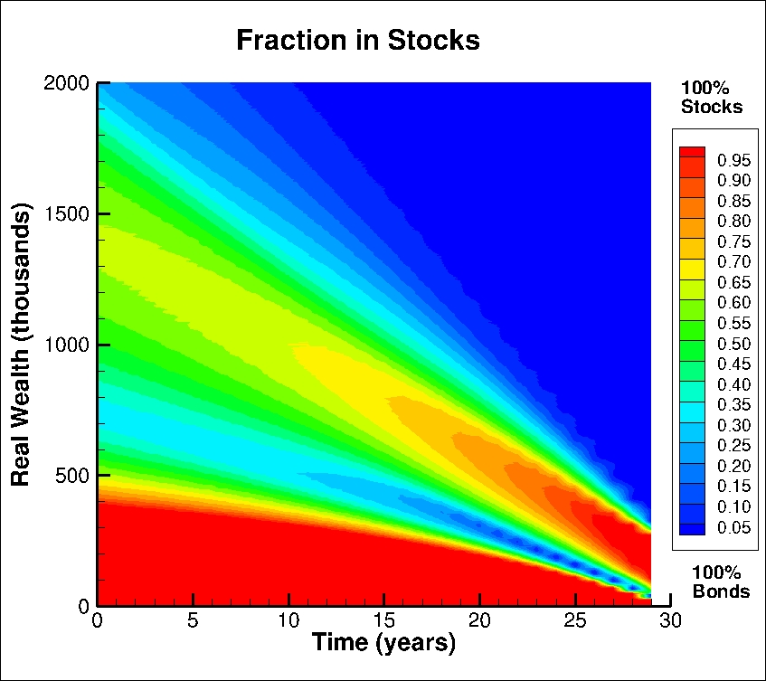
leads to the optimal strategy depicted in the heat map contained in Figure 10.3. For this example, if we set in problem (6.2), then . Recall that is set to be the value such that Prob as determined at time zero.2020 20 In all of our examples, we maximize ES at the level.
The structure of the heat map can be understood as follows. As , there are multiply-connected regions of all bond and all stock portfolios. For small values of wealth, the optimal strategy is to be fully invested in stocks, thus attempting to maximize ES. As wealth increases, Prob is small, and the investor switches to a portfolio that is heavily weighted towards the bond index to protect against the ES risk. If wealth increases further, the investor moves to investing more in stocks, in order to maximize withdrawals. Finally, for large values of wealth, there is little chance that . Since the withdrawals are capped at 80 per year, there is no incentive to take on any more risk. In this case, the stabilization term in equation (10.1) comes into effect. Since , this forces the strategy back into bonds.
It is useful to examine Figure 10.3 with reference to the median wealth shown in Figure 2(c). The initial wealth of is in the green region, with equity weight . As , the optimal control attempts to guide real wealth into the sweet spot between the lower blue zone and the upper red zone. The lower blue zone then acts as a barrier to lower wealth (i.e. running out of cash), since the portfolio becomes very stable with a large fraction of bonds. Above the lower blue zone, the allocation can vary considerably in an effort to maximize the total withdrawals, especially with a short time remaining.
Figure 10.3 also shows the effect of different starting values of wealth , keeping a minimum withdrawal of . For example, with the investor has no choice but to start with an investment of 100% in stocks and hope for the best. This is essentially a “Hail Mary” strategy, with little chance of success. On the other hand, if , the investor will start off being completely invested in bonds with very high probability of success.
11 Numerical Results: Historical Market
We continue to compute and store the optimal controls based on the parametric model (3.3-3.4) as in the synthetic market case. As a robustness test, we now calculate statistics using these stored controls, but with bootstrapped historical real return data rather than Monte Carlo simulations following the parametric model. We employ the stationary block bootstrap method (Politis and Romano 1994; Politis and White 2004) to generate many bootstrap simulated paths. A single path entails sampling randomly sized blocks from the historical data with replacement and pasting them together to cover the entire decumulation period of years.2121 21 Sampling in blocks helps to incorporate any serial correlation that is present in the data. The blocksize is generated randomly according to a geometric distribution with expected blocksize , which helps to mitigate the effects of a fixed block size.
We implement an algorithm from Patton et al. 2009 to determine the optimal expected blocksize for the bond and stock indexes separately. This indicates that the optimal expected blocksizes are 0.25 and 4.2 years for the stock and bond indexes respectively. However, to allow for possible contemporaneous dependence between the two indexes we use paired sampling to simultaneously draw returns from both series. Given the large difference in optimal expected blocksize for the two indexes, it is not obvious what should be done for paired sampling. One possibility is to use an average of the two estimates, suggesting about 2 years. We do this, but we also give results for a range of expected blocksizes as a robustness check.2222 22 Detailed pseudo-code for block bootstrap resampling can be found in Forsyth and Vetzal 2019.
In these bootstrap simulations, we continue to use the average historical real (uncompensated) drift for the T-bill index as the interest rate in the ARVA computation (2.3). This avoids the problem of fluctuating withdrawal amounts which are driven just by the bootstrap resampling methods. It is also a conservative approach since .
We first explore the effect of the expected blocksize . Table 11.1 shows the results computed by solving the pre-commitment EW-EW problem (6.2) in the synthetic market with and then using this control with block bootstrap resampling having various expected blocksizes . For ease of comparison, the table also provides the results for in the synthetic market that were previously shown in Table 10.4. The historical market results in Table 11.1 are generally similar to the corresponding synthetic market result, at least for values of between 0.5 and 2 years. The reported ES values for the historical market are consistently a bit better than in the synthetic market, while expected average withdrawals and median terminal wealth are quite comparable. However, the average of the median value of the equity weight is a bit higher, clustering at or above 0.4 for the historical market compared to 0.375 for the synthetic market. Results reported below use years, as this is (approximately) the average of the optimal expected blocksizes for the two indexes.
| ES () | ||||
| Synthetic Market (from Table 10.4) | ||||
| N/A | ||||
| Historical Market | ||||
| 0.25 years | ||||
| 0.5 years | ||||
| 1 year | ||||
| 2 years | ||||
| 5 years | ||||
Figure 11.1 shows the percentiles of the optimal controls, withdrawals and wealth throughout the decumulation period in the historical market with years. Figure 11.1 is very similar to the corresponding Figure 10.2 for the synthetic market. The median fraction invested in the stock index increases a little more sharply in Figure 11.1, and the 5th percentile of this fraction reaches zero a little later, but these are almost the only discernible differences. Overall, the close correspondence between the various panels of these two figures suggests that the parametric model used when solving for the optimal control is fairly robust as the historical market makes no assumptions about the processes followed by the stock and bond indexes.2323 23 However, this is not always true. In this case, ES (see Table 11.1 with years) is about . As we will see below, if we try to increase ES to higher values than this, then the controls do not appear to be robust.
We now compare in the historical market the same three strategies that were considered previously in the synthetic market of Section 10, i.e. constant withdrawals of with constant asset allocation weights, ARVA withdrawals with constant asset allocation weights, and ARVA withdrawals with optimal asset allocation. Appendix B provides tables of results for these strategies in the historical market with years; here we present plots based on those results.
The efficient frontiers of expected average withdrawals vs. ES in the historical market are plotted in Figure 2(a), which is analogous to Figure 1(a) for the synthetic market. As in Figure 1(a), Figure 2(a) shows that the ARVA withdrawal with constant weight asset allocation is a major improvement over the constant withdrawal with constant asset allocation weights. As expected, the optimal ARVA withdrawal strategy with optimal asset allocation continues to plot above the ARVA withdrawal strategy with constant weight asset allocation, indicating that optimal asset allocation can provide further significant enhancements. Although the general picture is the same here in the historical market as it was in the synthetic market, it is worth pointing out a couple of specific differences. First, consider the constant withdrawal strategy with constant asset allocation. In the synthetic market, the highest ES of about for an equity weight of 0.15 (see Table 10.1). This is the best available point, since withdrawals are constant. In the historical market, the corresponding ES is about for an equity weight of 0.40 (see Table B.1). However, Figure 1(a) indicates that in the synthetic market an ES of can be attained with expected average withdrawals of about 58 for the constant weight case and about 60 for the optimal asset allocation case. The corresponding values for the historical market in Figure 2(a) with an ES of are a little higher, about 61 for the constant weight case and around 63 for optimal asset allocation. These values do not constitute the largest gap between these two frontiers, but they do indicate that ARVA withdrawals (with either constant weight or optimal asset allocation) perform a bit better in the historical market relative to the synthetic market, at least for this level of ES. On the other hand, the performance of the constant withdrawal strategy is notably worse in the historical market.
A more direct comparison between the synthetic and historical markets is given in Figure 2(b) which plots the efficient frontiers of expected average withdrawals vs. ES for ARVA withdrawals with optimal asset allocation in both markets, with the optimal controls having of course been determined in the synthetic market. The frontier for the historical market plots above the frontier for the synthetic market if . However, the situation is reversed for . This suggests that it is unreliable to try to achieve very low ES risk in the actual market. This is not unreasonable, since in order to obtain ES values close to zero the optimal strategy will depend greatly on the stochastic market structure. Consequently, it appears that the synthetic market controls are not robust to parameter uncertainty for , although the controls do appear to be robust otherwise.
12 Conclusions
For both parametric model simulations and bootstrap resampling of the historical data, the ARVA withdrawal strategy with constant asset weights and minimum/maximum withdrawal constraints outperforms a constant withdrawal strategy with constant asset weights based on expected average withdrawals and expected shortfall criteria. This is consistent with results from the practitioner literature (Pfau 2015, e.g.) which show that withdrawal variability can significantly improve performance in cases with constant weight asset allocation. However, we also show that the ARVA withdrawal strategy can be further improved by dynamically choosing the equity weight. This strategy is determined by maximizing an expected total withdrawals/expected shortfall objective function using dynamic programming, assuming a parametric model of historical asset returns. As long as the desired expected shortfall is not unrealistically large, this strategy is robust to parameter misspecification, as verified by tests using bootstrapped resampled historical data.
Remarkably, the optimal dynamic ARVA strategy continues to outperform the constant withdrawal/constant weight strategy, even if the minimum ARVA withdrawal is set equal to the constant withdrawal in the latter strategy. These results indicate that if an investor in the decumulation stage of a DC plan is prepared to allow some variability in withdrawals, significant improvements can be obtained in both expected total withdrawals and expected shortfall.
Appendix
Appendix A Calibration of Model Parameters
This appendix discusses the estimation of the parameters of the jump diffusion processes for the stock and bond indexes given by equations (3.1), (3.3), (3.4), and (3.5). Recall that the equity index is the CRSP value-weighted stock index while the bond index is the CRSP 30-day T-bill index, and that both of these indexes are adjusted for inflation by using the CPI.
Jumps in the data are identified using the thresholding technique described in Mancini 2009 and Cont and Mancini 2011. Let be the detrended return in period , with period time interval . Suppose we have an estimate for the diffusive volatility component . Then we detect a jump in period if . We choose in this paper (note that is fixed). For justification for this parameter selection, see (Shimizu 2013; Dang and Forsyth 2016; Forsyth and Vetzal 2017). For details describing the recursive algorithm used to determine , see Forsyth and Vetzal 2017.
Figure 1(a) shows a histogram of the monthly returns from the value-weighted CRSP stock index, scaled to zero mean and unit standard deviation. We superimpose a standard normal density onto this histogram, as well as the fitted density for the double exponential jump diffusion model. Figure 1(b) shows the equivalent plot for the 30-day T-bill index.
During the sample period of 1926:1-2018:12 (monthly), the filtering algorithm identified 30 stock index jumps and 48 T-bill index jumps. Of these cases, just 5 were identified as occurring in the same month for both stocks and bonds, all in the 1930s. This supports our modelling assumption of no dependence between the jump intensities or jump distributions of the two indexes, though we do allow for correlated Brownian motion terms in the parametric model.
Appendix B Historical Market: Detailed Results
This appendix presents detailed results for the historical market bootstrap resampling tests with expected blocksize years. Table B.1 shows the results for a constant withdrawal () strategy with constant equity weight asset allocation, analogous to Table 10.1 in the synthetic market. Table B.2 gives results for ARVA withdrawals with constant equity weight asset allocation, analogous to Table 10.2 in the synthetic market. Finally, Table B.3 presents results in the historical market for ARVA withdrawals and optimal asset allocation (the optimal control is computed by solving the pre-commitment EW-ES problem (6.2) in the synthetic market). This table is analogous to Table 10.4 for the synthetic market.
| Equity Weight | ES () | Median |
|---|---|---|
| 0.0 | ||
| 0.1 | ||
| 0.2 | ||
| 0.3 | ||
| 0.4 | ||
| 0.5 | ||
| 0.6 | ||
| 0.7 | ||
| 0.8 | ||
| 0.9 | ||
| 1.0 |
| Equity Weight | ES () | Median[] | |
|---|---|---|---|
| 0.0 | |||
| 0.1 | |||
| 0.2 | |||
| 0.3 | |||
| 0.4 | |||
| 0.5 | |||
| 0.6 | |||
| 0.7 | |||
| 0.8 | |||
| 0.9 | |||
| 1.0 |
| ES () | Median[] | |||
|---|---|---|---|---|
| 0.1 | ||||
| 0.25 | ||||
| 0.4 | ||||
| 0.7 | ||||
| 1.0 | ||||
| 1.75 | ||||
| 2.5 | ||||
| 5.0 | ||||
| 10.0 | ||||
| 100.0 |
References
- Bengen (1994) Bengen, W. (1994). Determining withdrawal rates using historical data. Journal of Financial Planning 7, 171–180.
- Bengen (2001) Bengen, W. P. (2001). Conserving client portfolios during retirement, part IV. Journal of Financial Planning 14(5), 110–119.
- Carrick (2020) Carrick, R. (2020). Have a defined contribution pension plan? Here’s how to make the most of it. The Globe and Mail, Feb. 20, www.theglobeandmail.com/investing/personal-finance/article-how-not-to-mismanage-your-retirement-savings/.
- Cont and Mancini (2011) Cont, R. and C. Mancini (2011). Nonparametric tests for pathwise properties of semimartingales. Bernoulli 17, 781–813.
- Cui et al. (2019) Cui, X., J. Gao, Y. Shi, and S. Zhu (2019). Time-consistent and self-coordination strategies for multi-period mean-conditional-value-at-risk portfolio selection. European Journal of Operational Research 276, 781–789.
- Dang and Forsyth (2016) Dang, D.-M. and P. A. Forsyth (2016). Better than pre-commitment mean-variance portfolio allocation strategies: a semi-self-financing Hamilton-Jacobi-Bellman equation approach. European Journal of Operational Research 250, 827–841.
- Dang et al. (2017) Dang, D.-M., P. A. Forsyth, and K. R. Vetzal (2017). The 4% strategy revisited: a pre-commitment optimal mean-variance approach to wealth management. Quantitative Finance 17, 335–351.
- Finke et al. (2013) Finke, M., W. D. Pfau, and D. M. Blanchett (2013). The 4 percent rule is not safe in a low-yield world. Journal of Financial Planning 26(6), 46–55.
- Forsyth (2020a) Forsyth, P. A. (2020a). Multi-period mean CVAR asset allocation: Is it advantageous to be time consistent? SIAM Journal on Financial Mathematics 11:2, 358–384.
- Forsyth (2020b) Forsyth, P. A. (2020b). Optimal dynamic asset allocation for DC plan accumulation/decumulation: Ambition-CVAR. Insurance: Mathematics and Economics 93, 230–245.
- Forsyth (2020c) Forsyth, P. A. (2020c). A stochastic control approach to defined contribution plan decumulation: “the nastiest, hardest problem in finance”. Working paper, Cheriton School of Computer Science, University of Waterloo.
- Forsyth and Labahn (2019) Forsyth, P. A. and G. Labahn (2019). Monotone Fourier methods for optimal stochastic control in finance. Journal of Computational Finance 22:4, 25–71.
- Forsyth and Vetzal (2017) Forsyth, P. A. and K. R. Vetzal (2017). Dynamic mean variance asset allocation: Tests for robustness. International Journal of Financial Engineering 4, 1750021:1–1750021:37. DOI: 10.1142/S2424786317500219.
- Forsyth and Vetzal (2019) Forsyth, P. A. and K. R. Vetzal (2019). Optimal asset allocation for retirement savings: deterministic vs. time consistent adaptive strategies. Applied Mathematical Finance 26:1, 1–37.
- Forsyth et al. (2020) Forsyth, P. A., K. R. Vetzal, and G. Westmacott (2020). Optimal asset allocation for DC pension decumulation with a variable spending rule. ASTIN Bulletin 50, 419–447.
- Gao et al. (2016) Gao, J., Y. Xiong, and D. Li (2016). Dynamic mean-risk portfolio selection with multiple risk measures in continuous-time. European Journal of Operational Research 249, 647–656.
- Guyton and Klinger (2006) Guyton, J. T. and W. J. Klinger (2006). Decision rules and maximum initial withdrawal rates. Journal of Financial Planning 19(3), 48–58.
- Irlam (2014) Irlam, G. (2014). Portfolio size matters. Journal of Personal Finance 13(2), 9–16.
- Kou and Wang (2004) Kou, S. G. and H. Wang (2004). Option pricing under a double exponential jump diffusion model. Management Science 50, 1178–1192.
- Lin et al. (2015) Lin, Y., R. MacMinn, and R. Tian (2015). De-risking defined benefit plans. Insurance: Mathematics and Economics 63, 52–65.
- Ma and Forsyth (2016) Ma, K. and P. A. Forsyth (2016). Numerical solution of the Hamilton-Jacobi-Bellman formulation for continuous time mean variance asset allocation under stochastic volatility. Journal of Computational Finance 20(1), 1–37.
- MacDonald et al. (2013) MacDonald, B.-J., B. Jones, R. J. Morrison, R. L. Brown, and M. Hardy (2013). Research and reality: A literature review on drawing down retirement financial savings. North American Actuarial Journal 17, 181–215.
- MacMinn et al. (2014) MacMinn, R., P. Brockett, J. Wang, Y. Lin, and R. Tian (2014). The securitization of longevity risk and its implications for retirement security. In O. S. Mitchell, R. Maurer, and P. B. Hammond (Eds.), Recreating Sustainable Retirement, pp. 134–160. Oxford: Oxford University Press.
- Mancini (2009) Mancini, C. (2009). Non-parametric threshold estimation models with stochastic diffusion coefficient and jumps. Scandinavian Journal of Statistics 36, 270–296.
- Meeuwis (2020) Meeuwis, M. (2020). Wealth fluctations and risk preferences: Evidence from U.S. investor portfolios. Working paper, Washington University in St. Louis.
- Merton (2014) Merton, R. C. (2014). The crisis in retirement planning. Harvard Business Review July-August, 3–10.
- Milevsky and Young (2007) Milevsky, M. A. and V. R. Young (2007). Annuitization and asset allocation. Journal of Economic Dynamics and Control 31, 3138–3177.
- OECD (2019) OECD (2019). Pension Markets in Focus. www.oecd.org/daf/fin/private-pensions/pensionmarketsinfocus.htm.
- Patton et al. (2009) Patton, A., D. Politis, and H. White (2009). Correction to: automatic block-length selection for the dependent bootstrap. Econometric Reviews 28, 372–375.
- Peijnenburg et al. (2016) Peijnenburg, K., T. Nijman, and B. J. Werker (2016). The annuity puzzle remains a puzzle. Journal of Economic Dynamics and Control 70, 18–35.
- Pfau (2015) Pfau, W. D. (2015). Making sense out of variable spending strategies for retirees. Journal of Financial Planning 28(10), 42–51.
- Politis and Romano (1994) Politis, D. and J. Romano (1994). The stationary bootstrap. Journal of the American Statistical Association 89, 1303–1313.
- Politis and White (2004) Politis, D. and H. White (2004). Automatic block-length selection for the dependent bootstrap. Econometric Reviews 23, 53–70.
- Rockafellar and Uryasev (2000) Rockafellar, R. T. and S. Uryasev (2000). Optimization of conditional value-at-risk. Journal of Risk 2, 21–42.
- Shefrin and Thaler (1988) Shefrin, H. M. and R. H. Thaler (1988). The behavioral life-cycle hypothesis. Economic Inquiry 26, 609–643.
- Shimizu (2013) Shimizu, Y. (2013). Threshold estimation for stochastic differential equations with jumps. Proceedings of the 59th ISI World Statistics Conference, Hong Kong.
- Strub et al. (2019) Strub, M., D. Li, and X. Cui (2019). An enhanced mean-variance framework for robo-advising applications. SSRN 3302111.
- Thaler (1990) Thaler, R. H. (1990). Anomalies: Savings, fungibility, and mental accounts. Journal of Economic Perspectives 4(1), 193–205.
- Tretiakova and Yamada (2017) Tretiakova, I. and M. S. Yamada (2017). Autonomous portfolio: A decumulation investment strategy that will get you there. Journal of Retirement 5:2, 83–95.
- Van Staden et al. (2018) Van Staden, P., D.-M. Dang, and P. Forsyth (2018). Time-consistent mean-variance portfolio optimization: a numerical impulse control approach. Insurance: Mathematics and Economics 83, 9–28.
- Waring and Siegel (2015) Waring, M. B. and L. B. Siegel (2015). The only spending rule article you will ever need. Financial Analysts Journal 71(1), 91–107.
- Westmacott (2017) Westmacott, G. (2017). The retiree’s dilemma: the Deckards. PWL Capital White Paper, http://www.pwlcapital.com/retirees-dilemmma-deckards/.