¹¹footnotetext: School of Mathematical Sciences and Key Laboratory for Nonlinear Science, Fudan University, Shanghai 200433, P.R. China.

On asymptotic approximation of the modified Camassa-Holm equation in different space-time solitonic regions

Yiling YANG Thanks: Email address: 19110180006@fudan.edu.cn Engui FAN Thanks: Corresponding author and email address: faneg@fudan.edu.cn

Abstract

In this paper, we study the long time asymptotic behavior for the initial value problem of the modified Camassa-Holm (mCH) equation in the solitonic region

		$\displaystyle m_{t}+\left(m\left(u^{2}-u_{x}^{2}\right)\right)_{x}+\kappa u_{x}=0,\quad m=u-u_{xx},$
		$\displaystyle u(x,0)=u_{0}(x),$

where $\kappa$ is a positive constant. Based on the spectral analysis of the Lax pair associated with the mCH equation and scattering matrix, the solution of the Cauchy problem is characterized via the solution of a Riemann-Hilbert (RH) problem. Further using the $\overline{\partial}$ generalization of Deift-Zhou steepest descent method, we derive different long time asymptotic expansion of the solution $u(x,t)$ in different space-time solitonic region of $x/t$ . These asymptotic approximations can be characterized with an $N(\Lambda)$ -soliton whose parameters are modulated by a sum of localized soliton-soliton interactions as one moves through the region with diverse residual error order from $\overline{\partial}$ equation: $\mathcal{O}(|t|^{-1+2\rho})$ for $\xi=\frac{y}{t}\in(-\infty,-0.25)\cup(2,+\infty)$ and $\mathcal{O}(|t|^{-3/4})$ for $\xi=\frac{y}{t}\in(-0.25,2)$ . Our results also confirm the soliton resolution conjecture and asymptotically stability of N-soliton solutions for the mCH equation.

Keywords: Modified Camassa-Holm equation, Riemann-Hilbert problem, $\overline{\partial}$ steepest descent method, long time asymptotics, asymptotic stability, soliton resolution.

MSC: 35Q51; 35Q15; 37K15; 35C20.

1 Introduction

The inverse scattering transform (IST) procedure, as one of the most powerful tool to investigate solitons of nonlinear integrable models, was first discovered by Gardner, Green, Kruskal and Miura [1]. The modern version of IST is based on the dressing method proposed by Zakharov and Shabat, first in terms of the factorization of integral operators on a line into a product of two Volterra integral operators [2] and then using the Riemann-Hilbert (RH) problem [3]. In general, the initial value problems of integrable systems can be solved by suing IST or RH method only in the case of refectioness potentials. So a natural idea is to study the asymptotic behavior of solutions to integrable systems.

The study on the long-time behavior of nonlinear wave equations was first carried out with IST method by Manakov in 1974 [4]. Later, by using this method, Zakharov and Manakov gave the first result on the large-time asymptotic of solutions for the NLS equation with decaying initial value [5]. The IST method also worked for long-time behavior of integrable systems such as KdV, Landau-Lifshitz and the reduced Maxwell-Bloch system [6, 7, 8]. In 1993, Deift and Zhou developed a nonlinear steepest descent method to rigorously obtain the long-time asymptotics behavior of the solution for the MKdV equation by deforming contours to reduce the original Riemann-Hilbert (RH) problem to a model one whose solution is calculated in terms of parabolic cylinder functions [9]. Since then this method has been widely applied to the focusing NLS equation, KdV equation, Camassa-Holm equation,Degasperis-Procesi, Fokas-Lenells equation, Sasa-Satuma equation, short-pulse equation etc. [10, 11, 12, 13, 14, 15, 16, 17, 18, 19].

In recent years, McLaughlin and Miller further presented a $\bar{\partial}$ steepest descent method which combine steepest descent with $\bar{\partial}$ -problem rather than the asymptotic analysis of singular integrals on contours to analyze asymptotic of orthogonal polynomials with non-analytical weights [20, 21]. When it is applied to integrable systems, the $\bar{\partial}$ steepest descent method also has displayed some advantages, such as avoiding delicate estimates involving $L^{p}$ estimates of Cauchy projection operators, and leading the non-analyticity in the RH problem reductions to a $\bar{\partial}$ -problem in some sectors of the complex plane. Dieng and McLaughin used it to study the defocusing NLS equation under essentially minimal regularity assumptions on finite mass initial data [22]; This method was also successfully applied to prove asymptotic stability of N-soliton solutions to focusing NLS equation [23]; Jenkins et.al studied soliton resolution for the derivative nonlinear NLS equation for generic initial data in a weighted Sobolev space [24]. For finite density initial data, Cussagna and Jenkins improved $\bar{\partial}$ steepest descent method to study the asymptotic stability for defocusing NLS equation with non-zero boundary conditions [25]. Recently $\bar{\partial}$ steepest descent method has been successfully used to study the short pulse, three-wave, modifed Camassa-Holm and Fokas-Lenells equations [26, 27, 28, 29].

In the present paper, we study the long time asymptotic behavior for the initial value problem for the modified Camassa-Holm (mCH) equation:

		$\displaystyle m_{t}+\left(m\left(u^{2}-u_{x}^{2}\right)\right)_{x}+\kappa u_{x}=0,\quad m=u-u_{xx},$		(1.1)
		$\displaystyle u(x,0)=u_{0}(x),\quad x\in\mathbb{R},\ t>0,$		(1.2)

where $\kappa$ is a positive constant, and $u=u(x,t)$ is a real-valued function of $x$ and $t$ . The mCH equation (1.1) as a new integrable system was derived independently by Fokas [30], Fuchssteiner [31], Olver and Rosenau [32], and Qiao [33], where the equation was derived from the two-dimensional Euler system, and Lax pair, the M/W-shape solitons and peakon/cuspon solutions were presented. So the mCH equation (1.1) is also referred to as the Fokas-Olver-Rosenau-Qiao equation [34], but is mostly known as the mCH equation.

In recent years, the mCH equation (1.1) has attracted considerable interest due to its rich mathematical structure and remarkable properties such as algebro-geometric quasiperiodic solutions [34], Backlund transformation [35], conservative peakons [36, 37], local well-posedness for classical solutions and global weak solutions to (1.1) in Lagrangian coordinates [38] and solitary wave solutions [39]. Under a simple transformation

\displaystyle x=\tilde{x},\ \ t=\frac{2}{\kappa}\tilde{t},\ \ u(x,t)=\sqrt{\frac{\kappa}{2}}\tilde{u}(\tilde{x},\tilde{t}),

(1.3)

the mCH equation (1.1) becomes

\tilde{m}_{\tilde{t}}+\left(\tilde{m}\left(\tilde{u}^{2}-\tilde{u}_{\tilde{x}}^{2}\right)\right)_{\tilde{x}}+2\tilde{u}_{\tilde{x}}=0,\quad\tilde{m}=\tilde{u}-\tilde{u}_{xx}.

(1.4)

So without loss of generally, we fix $\kappa=2$ . Applying the scaling transformation

\displaystyle x=\epsilon\hat{x},\ \ t={\hat{t}}/{\epsilon},\ \ u(x,t)=\epsilon^{2}\hat{u}(\hat{x},\hat{t}),

(1.5)

and let $\epsilon\to 0$ , then the mCH reduces short pulse equation

\displaystyle u_{xt}=u+\frac{1}{6}(u^{3})_{xx}.

(1.6)

Recently, Boutet de Monvel, Kostenko, Shepelsky and Teschl developed a RH approach to the mCH equation (1.1) with nonzero boundary conditions [40]. They further present the results of the asymptotic analysis in the solitonless case for the two sectors $\frac{3}{4}<\frac{x}{t}<1,\ 1<\frac{x}{t}<3$ [42]. Xu and Fan applied Deift-Zhou steepest decedent method to obtain long-time asymptotic behavior of (1.1) with zero boundary conditions [41].

\displaystyle u(x,t)=f(x,t,\xi)t^{-1/2}+\mathcal{O}(t^{-1}\log t),

(1.7)

where $\xi=\frac{x}{t}$ , and $f$ has different structure for $\xi$ in different cases respectively.

In our results, for the weighted Sobolev initial data $u_{0}(x)\in H^{1,1}(\mathbb{R})$ , we obtain the leading order asymptotic approximation for the mCH equation (1.1) (see Theorem 1 in the section 9): when $\xi\in(-\infty,-0.25)\cup(2,+\infty)$ ,

\displaystyle u(x,t)=

\displaystyle=u^{r}(x,t;\tilde{\mathcal{D}})+\mathcal{O}(t^{-1+2\rho}),

(1.8)

and when $\xi\in(-0.25,2)$ ,

\displaystyle u(x,t)=u^{r}(x,t;\tilde{\mathcal{D}})+f_{11}t^{-1/2}+\mathcal{O}(t^{-3/4}).

(1.9)

Our results is different from it in [42, 41].

This paper is arranged as follows. In section 2, we recall some main results on the construction process of RH problem [41], which will be used to analyze long-time asymptotics of the mCH equation in our paper. In section 3, we shown that the reflection coefficient $r(z)$ belongs in $H^{1,1}(\mathbb{R})$ . In section 4, a $T(z)$ function is introduced to define a new RH problem for $M^{(1)}(z)$ , which admits a regular discrete spectrum and two triangular decompositions of the jump matrix near 0. In section 5, by introducing a matrix-valued function $R(z)$ , we obtain a mixed $\bar{\partial}$ -RH problem for $M^{(2)}(z)$ by continuous extension of $M^{(1)}(z)$ . In section 6, we decompose $M^{(2)}(z)$ into a model RH problem for $M^{R}(z)$ and a pure $\bar{\partial}$ Problem for $M^{(3)}(z)$ . The $M^{R}(z)$ can be obtained via an modified reflectionless RH problem $M^{(r)}(z)$ for the soliton components which is solved in Section 7 and an inner model $M^{lo}(z)$ for the stationary phase point $\xi_{k}$ which are approximated by parabolic cylinder model obtained in Section 10 when $\xi=\frac{y}{t}\in(-0.25,2)$ . But when $\xi=\frac{y}{t}\in(-\infty,-0.25)\cup(2,+\infty)$ , $M^{R}(z)=M^{(r)}(z)$ . This is a more simple case. In section 9, the error function can be computed with a small-norm RH problem. In Section 10, we analyze the $\bar{\partial}$ -problem for $M^{(3)}$ . Finally, in Section 11, based on the result obtained above, a relation formula is found

\displaystyle M(z)=M^{(3)}(z)E(z)M^{(r)}(z)R^{(2)}(z)^{-1}T(z)^{-\sigma_{3}},

from which we then obtain the long-time asymptotic behavior for the mch equation (1.1) via reconstruction formula.

2 The spectral analysis and the RH problem

2.1 Some notations

In this subsection, we fix some notations used this paper. $\sigma_{1}$ , $\sigma_{2}$ and $\sigma_{3}$ are Pauli matrices

\sigma_{1}=\left(\begin{array}[]{cc}0&1\\ 1&0\end{array}\right),\hskip 14.22636pt\sigma_{2}=\left(\begin{array}[]{cc}0&-i\\ i&0\end{array}\right),\hskip 14.22636pt\sigma_{3}=\left(\begin{array}[]{cc}1&0\\ 0&-1\end{array}\right).\hskip 14.22636pt

If $I$ is an interval on the real line $\mathbb{R}$ and $X$ is a Banach space, then $C^{0}(I,X)$ denotes the space of continuous functions on $I$ taking values in $X$ . It is equipped with the norm

\|f\|_{C^{0}(I,X)}=\sup_{x\in I}\|f(x)\|_{X}.

Moreover, denote $C^{0}_{B}(X)$ as a space of bounded continuous functions on $X$ .

If the entries $f_{1}$ and $f_{2}$ are in space $X$ , then we call vector $\vec{f}=(f_{1},f_{2})^{T}$ is in space $X$ with $\parallel\vec{f}\parallel_{X}\triangleq\parallel f_{1}\parallel_{X}+\parallel f_{2}\parallel_{X}$ . Similarly, if every entries of matrix $A$ are in space $X$ , then we call $A$ is also in space $X$ .

We introduce the normed spaces:

•

A weighted $L^{p}(\mathbb{R})$ space is specified by

$L^{p,s}(\mathbb{R})=\left\{f(x)\in L^{p}(\mathbb{R})|\hskip 2.84544pt|x|^{s}f(x)\in L^{p}(\mathbb{R})\right\};$

•

A Sobolev space is defined by

W^{k,p}(\mathbb{R})=\left\{f(x)\in L^{p}(\mathbb{R})|\hskip 2.84544pt\partial^{j}f(x)\in L^{p}(\mathbb{R})\text{ for }j=1,2,...,k\right\};

•

A weighted Sobolev space is defined by

H^{k,s}(\mathbb{R})=\left\{f(x)\in L^{2}(\mathbb{R})|\hskip 2.84544pt(1+|x|^{s})\partial^{j}f(x)\in L^{2}(\mathbb{R}),\text{ for }j=1,...,k\right\}.

And the norm of $f(x)\in L^{p}(\mathbb{R})$ and $g(x)\in L^{p,s}(\mathbb{R})$ are abbreviated to $\parallel f\parallel_{p}$ , $\parallel g\parallel_{p,s}$ respectively. In our paper, we only need the initial value $m(x,0)=u(x,0)-u_{xx}(x,0)$ in $H^{2,2}(\mathbb{R})$ .

2.2 Spectral analysis on the Lax pair

The mCH equation (1.1) is completely integrable and admits the Lax pair [41]

\Phi_{x}=X\Phi,\hskip 14.22636pt\Phi_{t}=T\Phi,

(2.1)

where

X=-\frac{k}{2}\sigma_{3}+\frac{i\lambda m(x,t)}{2}\sigma_{2},

T=\frac{k}{\lambda^{2}}\sigma_{3}+\frac{k}{2}\left(u^{2}-u_{x}^{2}\right)\sigma_{3}-i\left(\frac{u-ku_{x}}{\lambda}+\frac{\lambda}{2}\left(u^{2}-u_{x}^{2}\right)m\right)\sigma_{2},

with $k=\sqrt{1-\lambda^{2}}$ and $\lambda\in\mathbb{C}$ being a spectral parameter. The $X$ and $T$ of above Lax pair are traceless matrices, so it implies that the determinant of a matrix solution to (2.1) is independent of $x$ and $t$ . To avoid multi-valued case of eigenvalue $\lambda$ , we introduce a uniformization variable

z=k+\lambda,

(2.2)

and obtain two single-valued functions

k(z)=\frac{i}{2}(z-\frac{1}{z}),\hskip 14.22636pt\lambda(z)=\frac{1}{2}(z+\frac{1}{z}).

(2.3)

Usually we only use the $x$ -part of Lax pair to analyze the initial value problem. For example in section 3, we consider the case of $t=0$ to obtain the relationship of reflection coefficient and initial data. And the $t$ -part is often used to determine the time evolution of the scattering data by inverse scattering transform method. Here different from NLS and derivative NLS equations [22, 25, 23], the Lax pair (2.1) for the mCH equation has singularities at $\lambda=0,\infty$ and branch cut points $z=\pm i$ in the extended complex $\lambda$ -plane, so the asymptotic behavior of their eigenfunctions should be controlled. But the asymptotic behaviors of Lax pair (2.1) as $z\to\infty$ can’t be directly obtained. This difficulty is also appear in other WKI-type equation, and it is solved by appropriate transformation due to Boutet de Monvel and Shepelsky [46, 47]. This idea was also applied in [48, 41]. By using her consequence directly, we need to use different transformations respectively to analyze these singularities $z=i$ , $z=0$ and $z=\infty$ , and give a new scale to construct RH problem. Now we first consider the case $z=\infty$ , which is corresponding to $\lambda=\infty$ .

Case I: $z=\infty$
In order to control asymptotic behavior of the Lax pair (2.1) as $z\to\infty$ , we define

\displaystyle F(x,t)=\sqrt{\frac{q+1}{2q}}\left(\begin{array}[]{cc}1&\frac{-im}{q+1}\\ \frac{-im}{q+1}&1\end{array}\right),

and

p(x,t,z)=x-\int_{x}^{\infty}(q-1)dy-\frac{2t}{\lambda(z)^{2}},\ \ \ q=\sqrt{m^{2}+1}.

(2.6)

Making a transformation

\Phi_{\pm}=F\mu_{\pm}e^{-\frac{i}{4}(z-\frac{1}{z})p\sigma_{3}},

(2.7)

then we obtain a new Lax pair

		$\displaystyle(\mu_{\pm})_{x}=-\frac{i}{4}(z-\frac{1}{z})p_{x}[\sigma_{3},\mu_{\pm}]+P\mu_{\pm},$		(2.8)
		$\displaystyle(\mu_{\pm})_{t}=-\frac{i}{4}(z-\frac{1}{z})p_{t}[\sigma_{3},\mu_{\pm}]+L\mu_{\pm},$		(2.9)

where

		$\displaystyle P=\frac{im_{x}}{2q^{2}}\sigma_{1}+\frac{m}{2zq}\left(\begin{array}[]{cc}-im&1\\ -1&im\end{array}\right),$
		$\displaystyle L=\frac{im_{t}}{2q^{2}}\sigma_{1}-\frac{m\left(u^{2}-u_{x}^{2}\right)}{2zq}\left(\begin{array}[]{cc}-im&1\\ -1&im\end{array}\right)+\frac{\left(z^{2}-1\right)u_{x}}{z^{2}+1}\sigma_{1}$
		$\displaystyle-\frac{2zu}{\left(z^{2}+1\right)q}\left(\begin{array}[]{cc}-im&1\\ -1&im\end{array}\right)+\frac{2iz\left(z^{2}-1\right)}{\left(z^{2}+1\right)^{2}}\left(\begin{array}[]{cc}\frac{1}{q}-1&\frac{-im}{q}\\ \frac{im}{q}&1-\frac{1}{q}\end{array}\right).$

Moreover

\displaystyle\mu_{\pm}\sim I,\hskip 14.22636ptx\rightarrow\pm\infty.

(2.18)

The Lax pair (2.8)-(2.9) can be written in to a total differential form

d\left(e^{\frac{i}{4}(z-\frac{1}{z})p\hat{\sigma}_{3}}\mu_{\pm}\right)=e^{\frac{i}{4}(z-\frac{1}{z})p\hat{\sigma}_{3}}\left(Pdx+Ldt\right)\mu_{\pm},

(2.19)

which leads to two Volterra type integrals

\mu_{\pm}=I+\int_{x}^{\pm\infty}e^{-\frac{i}{4}(z-\frac{1}{z})(p(x)-p(y))\hat{\sigma}_{3}}P(y)\mu_{\pm}(y)dy.

(2.20)

Denote

\mu_{\pm}=\left(\left[\mu_{\pm}\right]_{1},\left[\mu_{\pm}\right]_{2}\right),

where $\left[\mu_{\pm}\right]_{1}$ and $\left[\mu_{\pm}\right]_{2}$ are the first and second columns of $\mu_{\pm}$ respectively. Then from (2.20), we can show that $\left[\mu_{-}\right]_{1}$ and $\left[\mu_{+}\right]_{2}$ are analysis in $\mathbb{C}^{+}$ ; $\left[\mu_{+}\right]_{1}$ and $\left[\mu_{-}\right]_{2}$ are analysis in $\mathbb{C}^{-}$ .

Proposition 1.

Jost functions $\mu_{\pm}$ admit three reduction conditions on the $z$ -plane:

The first symmetry reduction:

\mu_{\pm}(z)=\sigma_{2}\overline{\mu_{\pm}(\bar{z})}\sigma_{2}=\sigma_{1}\overline{\mu_{\pm}(-z)}\sigma_{1}.

(2.21)

The second symmetry reduction:

\mu_{\pm}(z)=F^{-2}\sigma_{2}\mu_{\pm}(-z^{-1})\sigma_{2},

(2.22)

Since $\Phi_{\pm}$ are two fundamental matrix solutions of the Lax pair (2.1), there exists a linear relation between $\Phi_{+}$ and $\Phi_{-}$ , namely

\Phi_{-}(z;x,t)=\Phi_{+}(z;x,t)S(z),\hskip 14.22636ptz\in\mathbb{R}\hskip 14.22636pt,

(2.23)

where $S(z)$ is called scattering matrix, and it is only depended on $z$

S(z)=\left(\begin{array}[]{cc}a(z)&-\overline{b(\bar{z})}\\[4.0pt] b(z)&\overline{a(\bar{z})}\end{array}\right),\hskip 14.22636pt\det[S(z)]=1.

(2.24)

Combing with (2.7), above equation trans to

\displaystyle\mu_{-}(z)=\mu_{+}(z)e^{-\frac{i}{4}(z-\frac{1}{z})p\hat{\sigma}_{3}}S(z).

(2.25)

Then $S(z)$ has following symmetry reduction:

S(z)=\overline{S(\bar{z}^{-1})}=\sigma_{3}S\left(-z^{-1}\right)\sigma_{3}.

(2.26)

And the reflection coefficients is defined by

r(z)=\frac{b(z)}{a(z)},

(2.27)

with symmetry reduction:

r(z)=\overline{r(\bar{z}^{-1})}=r(-z^{-1})=-\overline{r(-\bar{z})}.

(2.28)

From (2.23), $a(z)$ , $b(z)$ can be expressed by $\mu_{\pm}$ as

\displaystyle a(z)=\mu_{-}^{11}\overline{\mu_{+}^{11}}+\mu_{-}^{21}\overline{\mu_{+}^{21}},\hskip 14.22636ptb(z)=\overline{\mu_{-}^{11}\mu_{+}^{21}}-\overline{\mu_{-}^{21}\mu_{+}^{11}}.

(2.29)

So $a(z)$ is analytic on $\mathbb{C}^{+}$ . In addition, $\mu_{\pm}$ admit the asymptotics

\displaystyle\mu_{\pm}=I+\dfrac{D_{1}}{z}+\mathcal{O}(z^{-2}),\hskip 14.22636ptz\rightarrow\infty,

(2.30)

where the off-diagonal entries of the matrix $D_{1}(x,t)$ are

D_{12}(x,t)=-D_{21}(x,t)=\dfrac{m_{x}}{(1+m^{2})^{3/2}}.

(2.31)

From (2.30) and (2.34), we obtain the asymptotic of $a(z)$

\displaystyle a(z)=1+\mathcal{O}(z^{-1}),\hskip 14.22636ptz\rightarrow\infty.

(2.32)

The zeros of $a(z)$ on $\mathbb{R}$ are known to occur and they correspond to spectral singularities. They are excluded from our analysis in the this paper. To deal with our following work, we assume our initial data satisfy this assumption.

Assumption 1.

The initial data $u\in H^{4,2}(\mathbb{R})$ and it generates generic scattering data which satisfy that

1. a(z) has no zeros on $\mathbb{R}$ .

2. a(z) only has finite number of simple zeros.

And the proof of following proposition wil be given is section 3.

Proposition 2.

If the initial data $u\in H^{4,2}(\mathbb{R})$ , then $r(z)$ belongs to $H^{1,1}(\mathbb{R})$ .

Suppose that $a(z)$ has $N_{1}$ simple zeros $z_{1},...,z_{N_{1}}$ on $\{z\in\mathbb{C}^{+}:{\rm Im}z>0,|z|>1\}$ , and $N_{2}$ simple zeros $w_{1},...,w_{m}$ on the circle $\{z=e^{i\varphi}:\frac{\pi}{2}<\varphi<\pi\}$ . The symmetries (2.26) imply that

a(z_{n})=0\Leftrightarrow a(-\bar{z}_{n})=0\Leftrightarrow a\left(-\frac{1}{z_{n}}\right)=0\Leftrightarrow a\left(\frac{1}{\bar{z}}\right)=0,\hskip 14.22636ptn=1,...,N_{1},

and on the circle

a(w_{m})=0\Leftrightarrow a(-\bar{w}_{m})=0,\hskip 14.22636ptm=1,...,N_{2}.

So the zeros of $a(z)$ come in pairs. It is convenient to define zeros of $a(z)$ as $\zeta_{n}=z_{n}$ , $\zeta_{n}+N_{1}=-\bar{z}_{n}$ , $\zeta_{n+2N_{1}}=\bar{z}_{n}^{-1}$ and $\zeta_{n+3N_{1}}=-z_{n}^{-1}$ for $n=1,\cdot\cdot\cdot,N_{1}$ ; $\zeta_{m+4N_{1}}=w_{m}$ and $\zeta_{m+4N_{1}+N_{2}}=-\bar{w}_{m}$ for $m=1,\cdot\cdot\cdot,N_{2}$ . Then $\bar{\zeta}_{n}$ is the zeros of $\overline{a(\bar{z})}$ . Therefore, the discrete spectrum is

\mathcal{Z}=\left\{\zeta_{n},\ \bar{\zeta}_{n}\right\}_{n=1}^{4N_{1}+2N_{2}},

(2.33)

with $\zeta_{n}\in\mathbb{C}^{+}$ and $\bar{\zeta}_{n}\in\mathbb{C}^{-}$ . And the distribution of $\mathcal{Z}$ on the $z$ -plane is shown in Figure 1.

Figure 1: Distribution of the discrete spectrum

\mathcal{Z}

. The red one is unit circle.

Moreover, from trace formulae we have

a(z)=\prod_{j=1}^{4N_{1}+2N_{2}}\frac{z-\zeta_{j}}{z-\bar{\zeta}_{j}}\exp\left\{-\frac{1}{2\pi i}\int_{\mathbb{R}}\frac{\log(1+|r(s)|^{2})}{s-z}ds\right\}.

(2.34)

Then by taking $z\to\infty$ , it implies

0=\frac{1}{2\pi i}\int_{\mathbb{R}}\frac{\log(1+|r(s)|^{2})}{s}ds.

(2.35)

Case II: $z=0$ (corresponding to $\lambda\to\infty$ ).
From the symmetry condition in Proposition 1, we can obtain the property of $\mu(z)$ as $z\to 0$ . In addition, (2.32) and (2.26) imply $a(0)=1$ , which means $r(0)=0$ .

Case III: $z=\pm i$ (corresponding to $\lambda=0$ ).
Consider the Jost solutions of the Lax pair (2.1), which are restricted by the boundary conditions

\Phi_{\pm}\sim e^{(-\frac{k}{2}x+\frac{k}{\lambda^{2}}t)\sigma_{3}},\hskip 14.22636ptx\to\pm\infty.

(2.36)

Define a new transformation:

\mu^{0}_{\pm}=\Phi_{\pm}e^{(\frac{k}{2}x-\frac{k}{\lambda^{2}}t)\sigma_{3}},

(2.37)

with

\mu^{0}_{\pm}\sim I,\hskip 14.22636ptx\rightarrow\pm\infty.

Then the Lax pair (2.1) change to

		$\displaystyle(\mu^{0}_{\pm})_{x}=-\frac{k}{2}[\sigma_{3},\mu^{0}_{\pm}]+L_{0}\mu^{0}_{\pm},$		(2.38)
		$\displaystyle(\mu^{0}_{\pm})_{t}=\frac{k}{\lambda^{2}}[\sigma_{3},\mu^{0}_{\pm}]+M_{0}\mu^{0}_{\pm},$		(2.39)

with

		$\displaystyle L_{0}=\frac{\lambda mi}{2}\sigma_{2},$		(2.40)
		$\displaystyle M_{0}=\frac{\left(u^{2}-u_{x}^{2}\right)}{2}\left(\begin{array}[]{cc}k&-\lambda m\\ \lambda m&-k\end{array}\right)+\frac{u}{\lambda}\left(\begin{array}[]{cc}0&-1\\ 1&0\end{array}\right)+\frac{k}{\lambda}u_{x}\sigma_{1}.$

Similarly, we denote $\mu_{\pm}^{0}=\left(\left[\mu_{\pm}^{0}\right]_{1},\left[\mu^{0}_{\pm}\right]_{2}\right)$ . To reconstruct $u(x,t)$ , we analyze its asymptotic behavior as $z\to i$ :

\displaystyle\mu^{0}=I+(z-i)\left(\begin{array}[]{cc}0&-\frac{1}{2}(u+u_{x})\\ -\frac{1}{2}(u-u_{x})&0\end{array}\right)+\mathcal{O}\left((z-i)^{2}\right).

The relations (2.37) and (2.7) is

\mu_{\pm}(x,t,z)=F^{-1}(x,t)\mu^{0}_{\pm}e^{\frac{i}{4}(z-\frac{1}{z})c_{\pm}(x,t)\sigma_{3}},

(2.47)

where

\displaystyle c_{\pm}(x,t)=\int_{\pm\infty}^{x}(q-1)dy.

(2.48)

Further, taking $z\rightarrow i$ in (2.47) and combining it to (2.2), we get the asymptotic of $a(z)$ at $z\rightarrow i$ :

\displaystyle a(z)=e^{\frac{1}{2}\int_{\mathbb{R}}(q-1)dx}\left(1+\mathcal{O}\left((z-i)^{2}\right)\right),\hskip 8.5359pt\text{as }z\to i.

(2.49)

2.3 A RH problem

As shown in [41], denote norming constant $c_{n}=b_{n}/a^{\prime}(z_{n})$ . Then we have residue conditions as

\displaystyle\res_{z=z_{n}}\left[\frac{[\mu_{-}]^{1}(z)}{a(z)}\right]=c_{n}e^{-2k(z_{n})p(z_{n})}[\mu_{+}]^{2}(z_{n}),

(2.50)

For $m=1,...,N_{2}$ , there also have $c_{N_{1}+m}=b_{N_{1}+m}/a^{\prime}(w_{m})$ and

\displaystyle\res_{z=w_{m}}\left[\frac{[\mu_{-}]^{1}(z)}{a(z)}\right]=c_{N_{1}+m}e^{-2k(w_{n})p(w_{n})}[\mu_{+}]^{2}(w_{m}).

(2.51)

The symmetry of $a(z)$ and $\mu(z)$ in Proposition 1 leads to other norming constant for zeros of $a(z)$ . For brevity, we introduce a new constant $C_{n}$ as: for $n=1,...,N_{1}$ , $C_{n}=c_{n}$ , $C_{n+N_{1}}=\bar{c}_{n}$ $C_{n+2N_{1}}=-\bar{z}_{n}^{-2}\bar{c}_{n}$ and $C_{n+3N_{1}}=-z^{-2}_{n}c_{n}$ ; for $m=1,...,N_{2}$ , $C_{m+4N_{1}}=\bar{C}_{m+4N_{1}+N_{2}}=c_{m+N_{1}}$ , and the collection $\sigma_{d}=\left\{\zeta_{n},C_{n}\right\}^{4N_{1}+2N_{2}}_{n=1}$ is called the scattering data. define a sectionally meromorphic matrix

N(z)\triangleq N(z;x,t)=\left\{\begin{array}[]{ll}\left(\frac{\left[\mu_{-}\right]_{1}}{a(z)},\left[\mu_{+}\right]_{2}\right),&\text{as }z\in\mathbb{C}^{+},\\[12.0pt] \left(\left[\mu_{+}\right]_{1},\frac{\left[\mu_{-}\right]_{2}}{\overline{a(\bar{z})}}\right),&\text{as }z\in\mathbb{C}^{-},\\ \end{array}\right.

(2.52)

which solves the following RHP.

RHP 1.

Find a matrix-valued function $N(z)\triangleq N(z;x,t)$ which satisfies:

$\blacktriangleright$ Analyticity: $N(z)$ is meromorphic in $\mathbb{C}\setminus\mathbb{R}$ and has single poles;

$\blacktriangleright$ Symmetry: $N(z)=\sigma_{3}\overline{N(-\bar{z})}\sigma_{3}$ = $\sigma_{2}\overline{N(\bar{z})}\sigma_{2}$ = $F^{-2}\overline{N(-\bar{z}^{-1})}$ ;

$\blacktriangleright$ Jump condition: $N$ has continuous boundary values $N_{\pm}(z)$ on $\mathbb{R}$ and

N_{+}(z)=N_{-}(z)\tilde{V}(z),\hskip 14.22636ptz\in\mathbb{R},

(2.53)

where

\tilde{V}(z)=\left(\begin{array}[]{cc}1+|r(z)|^{2}&e^{-kp}\overline{r(z)}\\ e^{kp}r(z)&1\end{array}\right);

(2.54)

$\blacktriangleright$ Asymptotic behaviors:

		$\displaystyle N(z)=I+\mathcal{O}(z^{-1}),\hskip 14.22636ptz\rightarrow\infty,$		(2.55)
		$\displaystyle N(z)=F^{-1}\left[I+(z-i)\left(\begin{array}[]{cc}0&-\frac{1}{2}(u+u_{x})\\ -\frac{1}{2}(u-u_{x})&0\end{array}\right)\right]e^{\frac{1}{2}c_{+}\sigma_{3}}+\mathcal{O}\left((z-i)^{2}\right);$

$\blacktriangleright$ Residue conditions: $N(z)$ has simple poles at each point in $\mathcal{Z}\cup\bar{\mathcal{Z}}$ with:

		$\displaystyle\res_{z=\zeta_{n}}N(z)=\lim_{z\to\zeta_{n}}N(z)\left(\begin{array}[]{cc}0&0\\ c_{n}e^{-\sqrt{1-\lambda(\zeta_{n})^{2}}p(\zeta_{n})}&0\end{array}\right),$
		$\displaystyle\res_{z=\bar{\zeta}_{n}}N(z)=\lim_{z\to\bar{\zeta}_{n}}N(z)\left(\begin{array}[]{cc}0&-\bar{c}_{n}e^{\sqrt{1-\lambda(\bar{\zeta}_{n})^{2}}p(\bar{\zeta}_{n})}\\ 0&0\end{array}\right).$

The solution of mCH equation (1.1) is difficult to reconstruct , since $p(x,t,z)$ is still unknown. It has been a difficult problem when construct RHP of Camassa-Holm type equation until Boutet de Monvel and Shepelsky give the idea of changing the spatial variable in [46, 47] which successfully applied to short-wave-type equations in [48]. So following [41], to make the jump matrix become explicit, we introduce a new scale

y(x,t)=x-\int_{x}^{+\infty}\left(\sqrt{m(k,t)^{2}+1}-1\right)dk=x-c_{+}(x,t).

(2.62)

The price to pay for this is that the solution of the initial problem can be given only implicitly, or parametrically: it will be given in terms of functions in the new scale, whereas the original scale will also be given in terms of functions in the new scale. By the definition of the new scale $y(x,t)$ , we define

M(z)=M(z;y,t)\triangleq N(z;x(y,t),t),

(2.63)

Denote the phase function

\theta(z)=-\frac{1}{4}(z-\frac{1}{z})\left[\frac{y}{t}-\frac{8}{(z+\frac{1}{z})^{2}}\right],

(2.64)

and for convenience we denote $\theta_{n}=\theta(\zeta_{n})$ . Then, we can get the RH problem for the new variable $(y,t)$ .

RHP 2.

Find a matrix-valued function $M(z)=M(z;y,t)$ which satisfies:

$\blacktriangleright$ Analyticity: $M(z)$ is meromorphic in $\mathbb{C}\setminus\mathbb{R}$ and has single poles;

$\blacktriangleright$ Symmetry: $M(z)=\sigma_{3}\overline{M(-\bar{z})}\sigma_{3}$ = $\sigma_{2}\overline{M(\bar{z})}\sigma_{2}$ = $F^{-2}\overline{M(-\bar{z}^{-1})}$ ;

$\blacktriangleright$ Jump condition: $M$ has continuous boundary values $M_{\pm}$ on $\mathbb{R}$ and

M_{+}(z)=M_{-}(z)V(z),\hskip 14.22636ptz\in\mathbb{R},

(2.65)

where

V(z)=\left(\begin{array}[]{cc}1+|r(z)|^{2}&e^{2it\theta}\overline{r(z)}\\ e^{-2it\theta}r(z)&1\end{array}\right);

(2.66)

$\blacktriangleright$ Asymptotic behaviors:

		$\displaystyle M(z)=I+\mathcal{O}(z^{-1}),\hskip 14.22636ptz\rightarrow\infty,$		(2.67)
		$\displaystyle M(z)=F^{-1}\left[I+(z-i)\left(\begin{array}[]{cc}0&-\frac{1}{2}(u+u_{x})\\ -\frac{1}{2}(u-u_{x})&0\end{array}\right)\right]e^{\frac{1}{2}c_{+}\sigma_{3}}+\mathcal{O}\left((z-i)^{2}\right);$

$\blacktriangleright$ Residue conditions: $M(z)$ has simple poles at each point in $\mathcal{Z}$ with:

		$\displaystyle\res_{z=\zeta_{n}}M(z)=\lim_{z\to\zeta_{n}}M(z)\left(\begin{array}[]{cc}0&0\\ c_{n}e^{-2it\theta_{n}}&0\end{array}\right),$
		$\displaystyle\res_{z=\bar{\zeta}_{n}}M(z)=\lim_{z\to\bar{\zeta}_{n}}M(z)\left(\begin{array}[]{cc}0&-\bar{c}_{n}e^{2it\theta_{n}}\\ 0&0\end{array}\right).$

From the asymptotic behavior of the functions $\mu_{\pm}$ and (2), we arrive at following reconstruction formula of $u(x,t)=u(y(x,t),t)$ :

u(x,t)=u(y(x,t),t)=\lim_{z\to i}\frac{1}{z-i}\left(1-\dfrac{(M_{11}(z)+M_{21}(z))(M_{12}(z)+M_{22}(z))}{(M_{11}(i)+M_{21}(i))(M_{12}(i)+M_{22}(i))}\right),

(2.74)

where

x(y,t)=y+c_{+}(x,t)=y-\ln\left(\frac{M_{12}(i)+M_{22}(i)}{M_{11}(i)+M_{21}(i)}\right).

(2.75)

3 The reflection coefficient

We only consider the $x$ -part of Lax pair to give the proof of proposition (2) in this section. In fact, taking account of $t$ -part of Lax pair and though the standard direct scattering transform, then it deduce that $r(z)$ have linear time evolution: $r(z,t)=e^{\frac{i}{4\lambda^{2}(z)}(z-\frac{1}{z})}r(z,0)$ . So we can rewrite the steps as we shown in (Case I: $z=\infty$ ) at $t=0$ . Recall

\displaystyle F(x)=\sqrt{\frac{q+1}{2q}}\left(\begin{array}[]{cc}1&\frac{-im}{q+1}\\ \frac{-im}{q+1}&1\end{array}\right),

and

p(x)=x-\int_{x}^{\infty}\sqrt{m^{2}+1}-1dy.

(3.3)

Making a transformation

\Phi_{\pm}(x,z)=F(x)\mu_{\pm}(x,z)e^{-\frac{i}{4}(z-\frac{1}{z})p(x)\sigma_{3}},

(3.4)

then we obtain a new Lax pair

\displaystyle(\mu_{\pm})_{x}=-\frac{i}{4}(z-\frac{1}{z})p_{x}[\sigma_{3},\mu_{\pm}]+P\mu_{\pm},

(3.5)

where

\displaystyle P(x)=\frac{im_{x}}{2\left(M^{(2)}+1\right)}\sigma_{1}+\frac{1}{2z}\frac{m}{q}\left(\begin{array}[]{cc}-im&1\\ -1&im\end{array}\right).

Moreover

\displaystyle\mu_{\pm}\sim I,\hskip 14.22636ptx\rightarrow\pm\infty.

(3.8)

The standard AKNS method starts with the following two Volterra integral equations

\mu_{\pm}(x,z)=I+\int_{x}^{\pm\infty}e^{-\frac{i}{4}(z-\frac{1}{z})(p(x)-p(y))\hat{\sigma}_{3}}P(y)\mu_{\pm}(y,z)dy.

(3.9)

To obtain our result, we need estimates on the $L^{2}$ -integral property of $\mu_{\pm}(z)$ and their derivatives. However, because of the factor $1/z$ in the spectral problem (3.5), we divided our approach into two cases: $|z|>1$ and $|z|<1$ . And following functional analysis results, namely estimates for Volterra-type integral equations (3.9) useful in the analysis of direct scattering map.

Lemma 1.

For $f(x)\in L^{1}(\mathbb{R})$ , following inequality hold.

		$\displaystyle\sup_{\pm x>0}\left(\int_{1}^{+\infty}\|\int_{x}^{\pm\infty}\frac{f(y)}{z}dy\|^{2}dz\right)^{1/2}\lesssim\parallel f\parallel_{1};$		(3.10)
		$\displaystyle\left(\int_{0}^{\pm\infty}\int_{1}^{+\infty}\|\int_{x}^{\pm\infty}\frac{f(y)}{z}dy\|^{2}dzdx\right)^{1/2}\lesssim\parallel f\parallel_{1,1/2}.$		(3.11)

Lemma 2.

$f(k)$ is a function on ( $\mathbb{R}$ ). Denote $\eta=z-\frac{1}{z}$ , with $dz=\left(\frac{1}{2}+\frac{\eta}{\sqrt{4+\eta^{2}}}\right)d\eta$ .Let $f(z)=g(z-\frac{1}{z})=g(\eta)$ , then

\displaystyle\int_{1}^{+\infty}|f(z)|^{2}dz=\int_{0}^{+\infty}|g(\eta)|^{2}\left(\frac{1}{2}+\frac{\eta}{\sqrt{4+\eta^{2}}}\right)d\eta\lesssim\int_{\mathbb{R}}|g(\eta)|^{2}d\eta.

(3.12)

Lemma 3.

For $\psi(\eta)\in L^{2}(\mathbb{R})$ , $f(x)\in L^{2,1/2}(\mathbb{R})$ , following inequality hold.

$\displaystyle\|\int_{\mathbb{R}}\int_{x}^{\pm\infty}f(y)e^{-\frac{i}{2}\eta(p(x)-p(y))}\psi(\eta)dyd\eta\|$	$\displaystyle=\|\int_{x}^{\pm\infty}f(y)\psi(\frac{1}{2}(p(x)-p(y)))dy\|$
	$\displaystyle\lesssim\left(\int_{x}^{\pm\infty}\|f(y)\|^{2}dy\right)^{1/2}\parallel\psi\parallel_{2};$	(3.13)
$\displaystyle\int_{0}^{\pm\infty}\int_{\mathbb{R}}\|\int_{x}^{\pm\infty}f(y)e^{-\frac{i}{2}\eta(p(x)-p(y))}$	$\displaystyle dy\|^{2}d\eta dx\leq\parallel f\parallel_{2,1/2}^{2}.$	(3.14)

The proof of above lemmas are trivial. In lemma 3, let $s=\frac{p(x)-p(y)}{2}$ with $ds=\sqrt{m^{2}+1}dy$ , then

\displaystyle\left(\int_{x}^{\pm\infty}|\psi(\frac{p(x)-p(y)}{2})|^{2}dy\right)^{1/2}\leq\left(\int_{\mathbb{R}}\frac{|\psi(s)|^{2}}{\sqrt{m^{2}+1}}ds\right)^{1/2}\lesssim\parallel\psi\parallel_{2}.

(3.15)

And we omit the rest part of prove.

3.1 Large-z Estimates

From the symmetry reduction (2.21), we will only consider $[\mu_{\pm}]_{1}(x,z)$ for $z\in(1,+\infty)$ . For the sake of brevity, denote

\displaystyle[\mu_{\pm}]_{1}(x,z)-e_{1}\triangleq n_{\pm}(x,z)=\left(\begin{array}[]{cc}n_{\pm}^{1}\\ n_{\pm}^{2}\end{array}\right),

where $e_{1}$ is identity vector $(1,0)^{T}$ . And we abbreviate $C_{B}^{0}(\mathbb{R}^{\pm}\times(1,+\infty))$ , $C^{0}(\mathbb{R}^{\pm},L^{2}(1,+\infty))$ , $L^{2}(\mathbb{R}^{\pm}\times(1,+\infty))$ to $C_{B}^{0}$ , $C^{0}$ , $L^{2}_{xz}$ respectively. Introduce the integral operator $T_{\pm}$ :

\displaystyle T_{\pm}(f)(x,z)=\int_{x}^{\pm\infty}K_{\pm}(x,y,z)f(y,z)dy,

(3.18)

where integral kernel $K_{\pm}(x,y,z)$ is

		$\displaystyle K_{\pm}(x,y,z)=\left(\begin{array}[]{cc}1&0\\ 0&e^{-\frac{i}{2}(z-1/z)(p(x)-p(y))}\end{array}\right)P$
		$\displaystyle=\frac{im_{x}}{2\left(M^{(2)}+1\right)}\left(\begin{array}[]{cc}0&1\\ -e^{-\frac{i}{2}(z-1/z)(p(x)-p(y))}&0\end{array}\right)$
		$\displaystyle+\frac{1}{2z}\frac{m}{q}\left(\begin{array}[]{cc}-im&1\\ -e^{-\frac{i}{2}(z-1/z)(p(x)-p(y))}&e^{-\frac{i}{2}(z-1/z)(p(x)-p(y))}im\end{array}\right).$

Then (3.5) trans to

\displaystyle n_{\pm}=T_{\pm}(e_{1})+T_{\pm}(n_{\pm}).

(3.25)

To obtain the $z$ -derivative property of $n_{\pm}$ , we take the $z$ -derivative of above equation and get

\displaystyle[n_{\pm}]_{z}=n_{\pm}^{1}+T_{\pm}([n_{\pm}]_{z}),\hskip 14.22636ptn_{\pm}^{1}=[T_{\pm}]_{z}(e_{1})+[T_{\pm}]_{z}(n_{\pm}).

(3.26)

$[T_{\pm}]_{z}$ is also a integral operator with integral kernel $[K_{\pm}]_{z}(x,y,z)$ :

	$\displaystyle[K_{\pm}]_{z}(x,y,z)=$	$\displaystyle-\frac{i(p(x)-p(y))}{2}\frac{im_{x}}{2\left(M^{(2)}+1\right)}\left(\begin{array}[]{cc}0&0\\ -e^{-\frac{i}{2}(z-1/z)(p(x)-p(y))}&0\end{array}\right)$
		$\displaystyle-\frac{1}{z}\frac{mi}{4q}(p(x)-p(y))e^{-\frac{i}{2}(z-1/z)(p(x)-p(y))}\left(\begin{array}[]{cc}0&0\\ -1&im\end{array}\right)$
		$\displaystyle-\frac{1}{z^{2}}\frac{i(p(x)-p(y))}{2}\frac{im_{x}}{2\left(M^{(2)}+1\right)}\left(\begin{array}[]{cc}0&0\\ -e^{-\frac{i}{2}(z-1/z)(p(x)-p(y))}&0\end{array}\right)$
		$\displaystyle-\frac{1}{z^{2}}\frac{m}{q}\left(\begin{array}[]{cc}-im&1\\ -e^{-\frac{i}{2}(z-1/z)(p(x)-p(y))}&e^{-\frac{i}{2}(z-1/z)(p(x)-p(y))}im\end{array}\right)$
		$\displaystyle-\frac{1}{z^{3}}\frac{mi}{4q}(p(x)-p(y))e^{-\frac{i}{2}(z-1/z)(p(x)-p(y))}\left(\begin{array}[]{cc}0&0\\ -1&im\end{array}\right).$

Lemma 4.

$T_{\pm}$ and $[T_{\pm}]_{z}$ are integral operators defined above, then $T_{\pm}(e_{1})(x,z)\in C_{B}^{0}\cap C^{0}\cap L^{2}_{xz}$ and $[T_{\pm}]_{z}(e_{1})(x,z)\in C^{0}\cap L^{2}_{xz}$ .

Proof.

$T_{\pm}(e_{1})(x,z)$ is given by

	$\displaystyle T_{\pm}(e_{1})(x,z)=$	$\displaystyle\int_{x}^{\pm\infty}\frac{im_{x}}{2\left(M^{(2)}+1\right)}\left(\begin{array}[]{cc}0\\ -e^{-\frac{i}{2}(z-1/z)(p(x)-p(y))}\end{array}\right)dy$
		$\displaystyle+\frac{1}{2z}\int_{x}^{\pm\infty}\frac{m}{q}\left(\begin{array}[]{cc}-im\\ -e^{-\frac{i}{2}(z-1/z)(p(x)-p(y))}\end{array}\right)dy.$

It immediately derives to

\displaystyle|T_{\pm}(e_{1})(x,z)|\lesssim\parallel m\parallel_{2}^{2}+\parallel m\parallel_{1}.

(3.41)

And from lemma 1, we only need to estimate the first item of $T_{\pm}(e_{1})(x,z)$ . Let $\eta=z-\frac{1}{z}$ , with $dk=\left(\frac{1}{2}+\frac{\eta}{\sqrt{4+\eta^{2}}}\right)d\eta$ . Then from lemma 2, we only need to prove the first integral of (3.1):

H_{1}(x,\eta)\triangleq\int_{x}^{\pm\infty}\frac{im_{x}}{2\left(M^{(2)}+1\right)}e^{-\frac{i}{2}\eta(p(x)-p(y))}dy\in C^{0}(\mathbb{R}^{\pm},L^{2}(\mathbb{R}))\cap L^{2}(\mathbb{R}^{\pm}\times\mathbb{R}).

From lemma 3,

\displaystyle\parallel H_{1}(x,\eta)\parallel_{C^{0}}\lesssim\parallel m_{x}\parallel_{2},\hskip 14.22636pt\parallel H_{1}(x,\eta)\parallel_{L^{2}_{xz}}\lesssim\parallel m_{x}\parallel_{2,1/2}.

(3.42)

And $[T_{\pm}]_{z}(e_{1})(x,z)$ is given by

	$\displaystyle[T_{\pm}]_{z}(e_{1})(x,z)=$	$\displaystyle-\int_{x}^{\pm\infty}\frac{i(p(x)-p(y))}{2}\frac{im_{x}}{2\left(M^{(2)}+1\right)}\left(\begin{array}[]{cc}0&0\\ -e^{-\frac{i}{2}(z-1/z)(p(x)-p(y))}&0\end{array}\right)dy$
		$\displaystyle-\int_{x}^{\pm\infty}\frac{1}{z}\frac{mi}{4q}(p(x)-p(y))e^{-\frac{i}{2}(z-1/z)(p(x)-p(y))}\left(\begin{array}[]{cc}0&0\\ -1&im\end{array}\right)$
		$\displaystyle-\frac{1}{z^{2}}\frac{i(p(x)-p(y))}{2}\frac{im_{x}}{2\left(M^{(2)}+1\right)}\left(\begin{array}[]{cc}0&0\\ -e^{-\frac{i}{2}(z-1/z)(p(x)-p(y))}&0\end{array}\right)$
		$\displaystyle-\frac{1}{z^{2}}\frac{m}{q}\left(\begin{array}[]{cc}-im&1\\ -e^{-\frac{i}{2}(z-1/z)(p(x)-p(y))}&e^{-\frac{i}{2}(z-1/z)(p(x)-p(y))}im\end{array}\right)$
		$\displaystyle-\frac{1}{z^{3}}\frac{mi}{4q}(p(x)-p(y))e^{-\frac{i}{2}(z-1/z)(p(x)-p(y))}\left(\begin{array}[]{cc}0&0\\ -1&im\end{array}\right)dy.$

Similarly from lemma 1, we only need to evaluate the first integral. Denote $\eta=z-\frac{1}{z}$ and

H_{2}(x,\eta)=\int_{x}^{\pm\infty}\frac{i}{2}(p(x)-p(y))\frac{im_{x}}{2\left(M^{(2)}+1\right)}e^{-\frac{i}{2}\eta(p(x)-p(y))}dy.

Note that $|p(x)-p(y)|\leq|x-y|+\parallel m\parallel_{1}.$ Then it can be bound by analogy with $H_{1}$

		$\displaystyle\parallel H_{2}(x,\eta)\parallel_{C^{0}}\lesssim\parallel m_{x}\parallel_{2,1}+\parallel m_{x}\parallel_{2}\parallel m\parallel_{1},$		(3.53)
		$\displaystyle\parallel H_{2}(x,\eta)\parallel_{L^{2}_{xz}}\lesssim\parallel m_{x}\parallel_{2,3/2}+\parallel m_{x}\parallel_{2,1/2}\parallel m\parallel_{1}.$		(3.54)

∎

The operator $T_{\pm}$ , and $[T_{\pm}]_{k}$ induce linear mappings, which proposition are given in next lemma.

Lemma 5.

The integral operator $T_{\pm}$ maps $C_{B}^{0}\cap C^{0}\cap L^{2}_{xz}$ to itself while its $z$ -derivative $[T_{\pm}]_{k}$ is a integral operator on $C^{0}\cap L^{2}_{xz}$ . Moreover, $(I-T^{\pm})^{-1}$ exists as a bounded operator on $C_{B}^{0}\cap C^{0}\cap L^{2}_{xz}$ .

Proof.

In fact, (3.1) leads to

\displaystyle|K_{\pm}(x,y,z)|=|P(y,z)|.

(3.55)

Accordingly, for any $f(x,z)\in C_{B}^{0}(\mathbb{R}^{\pm}\times(1,+\infty))$ ,

\displaystyle|T_{\pm}(f)(x,z)|\leq\int_{x}^{\pm\infty}|P(y,z)|dy\parallel f\parallel_{C_{B}^{0}}.

(3.56)

Denote $K^{n}_{\pm}$ is the integral kernel of Volterra operator $[T_{\pm}]^{n}$ as

\displaystyle K^{n}_{\pm}(x,y,z)=\int_{x}^{y}\int_{y_{1}}^{y}...\int_{y_{n-2}}^{z}K_{\pm}(x,y_{1},z)K_{\pm}(y_{1},y_{2},z)...K_{\pm}(y_{n-1},y,z)dy_{n-1}...dy_{1},

(3.57)

with

\displaystyle|K^{n}_{\pm}(x,y,z)|\leq\frac{1}{(n-1)!}\left(\int_{x}^{\pm\infty}|P(y,z)|dy\right)^{n-1}|P(y,z)|.

(3.58)

Then the standard Volterra theory gives the following operator norm:

\displaystyle\parallel(I-T_{\pm})^{-1}\parallel_{\mathcal{B}(C_{B}^{0})}\leq e^{\int_{0}^{\pm\infty}|P(y,1)|dy}.

(3.59)

Analogously, $T_{\pm}$ is a bounded operator on $C^{0}$ with

\displaystyle\parallel(I-T_{\pm})^{-1}\parallel_{\mathcal{B}(C^{0})}\leq e^{\int_{\mathbb{R}}|P(y,1)|dy}.

(3.60)

By some minute modifications, there is similar boundedness result for $T_{\pm}$ on $L^{2}_{xz}$ with

		$\displaystyle\parallel T_{\pm}\parallel_{\mathcal{B}(L^{2}_{xz})}\leq\int_{\mathbb{R}}\|yP^{2}(y,1)\|dy;$		(3.61)
		$\displaystyle\parallel(I-T_{\pm})^{-1}\parallel_{\mathcal{B}(L^{2}_{xz})}\leq e^{\int_{\mathbb{R}}\|P(y,1)\|dy}\int_{\mathbb{R}}\|yP^{2}(y,1)\|dy.$		(3.62)

∎

Then from above lemma,

\parallel[T_{\pm}]_{z}(n_{\pm})\parallel_{C^{0}}\leq\parallel[T_{\pm}]_{z}\parallel_{\mathcal{B}(C^{0})}\parallel n_{\pm}\parallel_{L^{2}_{xz}},\parallel[T_{\pm}]_{z}(n_{\pm})\parallel_{L^{2}_{xz}}\leq\parallel[T_{\pm}]_{z}\parallel_{\mathcal{B}(L^{2}_{xz})}\parallel n_{\pm}\parallel_{C_{B}^{0}},

which implies $n_{\pm}^{1}\in C^{0}\cap L^{2}_{xz}$ . Since the operator $(I-T_{\pm})^{-1}$ exist, the equations (3.25)-(3.26) are solvable with:

		$\displaystyle n_{\pm}(x,z)=(I-T_{\pm})^{-1}(T_{\pm}(e_{1}))(x,z),$		(3.63)
		$\displaystyle n_{z}^{\pm}(x,z)=(I-T_{\pm})^{-1}([T_{\pm}]_{z}(e_{1})+T_{\pm}([n_{\pm}]_{z}))(x,z).$		(3.64)

Combining above Lemmas and the definition of $n_{\pm}$ (3.1), we immediately obtain the following property of $\mu_{\pm}(x,z)$ .

Proposition 3.

Suppose that $u\in H^{4,2}(\mathbb{R})$ , then $\mu_{\pm}(0,z)-I$ belongs in $C_{B}^{0}(1,+\infty)\cap L^{2}(1,+\infty)$ , while its $z$ -derivative $[\mu_{\pm}(0,z)]_{z}$ is in $L^{2}(1,+\infty)$ .

3.2 Small-z Estimates

Analogously, we will only consider $n_{\pm}(x,z)$ for $z\in(0,1)$ . Consider the change of variable: $z\in(0,1)\to\gamma=\frac{1}{z}\in(1,+\infty)$ . From proposition 1, we have

\displaystyle|[\mu_{\pm}]_{1}(x,z)|=|[\sigma_{2}F(x)^{2}\mu_{\pm}(x,\gamma)\sigma_{2}]_{1}|\lesssim|[\mu_{\pm}]_{1}(x,\gamma)|.

(3.65)

Then the boundedness of $n_{\pm}(x,z)$ of $z\in(0,1)$ follows immediately. Simple calculation gives that for $f(\gamma)\triangleq g(\frac{1}{z})$ ,

\displaystyle\int_{0}^{1}|g(\frac{1}{z})|^{2}dz=\int_{1}^{+\infty}\frac{|f(\gamma)|^{2}}{\gamma^{2}}d\gamma\leq\int_{1}^{+\infty}|f(\gamma)|^{2}d\gamma.

(3.66)

So $n_{\pm}(x,z)\in C^{0}(\mathbb{R}^{\pm},L^{2}(0,1))\cap L^{2}(\mathbb{R}^{\pm}\times(0,1))$ is equivalent to $\mu_{\pm}(x,\gamma)$ in $C^{0}(\mathbb{R}^{\pm},L^{2}(1,+\infty)_{\gamma})\cap L^{2}(\mathbb{R}^{\pm}\times(1,+\infty)_{\gamma})$ which obtained from proposition 3. However,

\displaystyle\int_{0}^{1}|g^{\prime}(\frac{1}{z})|^{2}dz=\int_{1}^{+\infty}|f^{\prime}(\gamma)|^{2}\gamma^{2}d\gamma.

(3.67)

Hence, our goal is to show that $[n_{\pm}]_{z}(x,\gamma)$ in $C^{0}(\mathbb{R}^{\pm},L^{2,1}(1,+\infty)_{\gamma})\cap L^{2,1}(\mathbb{R}^{\pm}\times(1,+\infty)_{\gamma})$ . From (3.26), it is sufficiently to show $\gamma[T_{\pm}]_{\gamma}(e_{1})$ and $\gamma[T_{\pm}]_{\gamma}(n_{\pm})$ in $C^{0}(\mathbb{R}^{\pm},L^{2}(1,+\infty)_{\gamma})\cap L^{2}(\mathbb{R}^{\pm}\times(1,+\infty)_{\gamma})$ . For any bounded continuous function $f(x,\gamma)$ on $C_{B}^{0}(\mathbb{R}^{\pm}\times(1,+\infty)_{\gamma})$ ,

\displaystyle|\gamma[T_{\pm}]_{\gamma}(f)(x,\gamma)|\leq|\int_{x}^{\pm\infty}\gamma[K_{\pm}]_{\gamma}(1,1)^{T}dy|\parallel f\parallel_{C_{B}^{0}(\mathbb{R}^{\pm}\times(1,+\infty)_{\gamma})}.

(3.68)

Consequently, we just need to prove the $L^{2}$ -integrability of $|\int_{x}^{\pm\infty}\gamma[K_{\pm}]_{\gamma}dy|$ in following lemma.

Lemma 6.

Suppose that $u\in H^{4,2}(\mathbb{R})$ , then $\int_{x}^{\pm\infty}\gamma[K_{\pm}]_{\gamma}(1,1)^{T}dy$ belongs to $C^{0}(\mathbb{R}^{\pm},L^{2}(1,+\infty)_{\gamma})\cap L^{2}(\mathbb{R}^{\pm}\times(1,+\infty)_{\gamma})$ .

Proof.

Recall (3.1) and have

$\displaystyle\gamma[K_{\pm}]_{\gamma}(x,y,\gamma)=$	$\displaystyle-\gamma\frac{i}{2}(p(x)-p(y))\frac{im_{x}}{2\left(M^{(2)}+1\right)}\left(\begin{array}[]{cc}0&0\\ -e^{-\frac{i}{2}(\gamma-1/\gamma)(p(x)-p(y))}&0\end{array}\right)$
	$\displaystyle-\frac{mi}{4q}(p(x)-p(y))e^{-\frac{i}{2}(\gamma-1/\gamma)(p(x)-p(y))}\left(\begin{array}[]{cc}0&0\\ -1&im\end{array}\right)$
	$\displaystyle-\frac{1}{\gamma}K^{0}_{\pm}(x,y,\gamma),$	(3.73)

where

	$\displaystyle K^{0}_{\pm}(x,y,\gamma)=$	$\displaystyle-\frac{i(p(x)-p(y))}{2}\frac{im_{x}}{2\left(M^{(2)}+1\right)}\left(\begin{array}[]{cc}0&0\\ -e^{-\frac{i}{2}(\gamma-1/\gamma)(p(x)-p(y))}&0\end{array}\right)$
		$\displaystyle-\frac{m}{q}\left(\begin{array}[]{cc}-im&1\\ -e^{-\frac{i}{2}(\gamma-1/\gamma)(p(x)-p(y))}&e^{-\frac{i}{2}(\gamma-1/\gamma)(p(x)-p(y))}im\end{array}\right)$
		$\displaystyle-\frac{1}{\gamma}\frac{mi}{4q}(p(x)-p(y))e^{-\frac{i}{2}(\gamma-1/\gamma)(p(x)-p(y))}\left(\begin{array}[]{cc}0&0\\ -1&im\end{array}\right).$

Then from lemma 1, we have $\int_{x}^{\pm\infty}\frac{1}{\gamma}K^{0}_{\pm}(x,y,\gamma)(1,1)^{T}dy\in C^{0}(\mathbb{R}^{\pm},L^{2}(1,+\infty)_{\gamma})\cap L^{2}(\mathbb{R}^{\pm}\times(1,+\infty)_{\gamma})$ right away. For the second item of $\gamma[K_{\pm}]_{\gamma}$ , we multiply it by $(1,1)^{T}$ and obtain

\displaystyle\gamma[K_{\pm}]_{\gamma}(1,1)^{T}=-\frac{mi}{4q}(p(x)-p(y))e^{-\frac{i}{2}(\gamma-1/\gamma)(p(x)-p(y))}\left(\begin{array}[]{cc}0\\ -1+im\end{array}\right).

Then we denote

\displaystyle f_{1}(x,y)=\frac{mi}{4q}(p(x)-p(y))(1-im).

(3.82)

Introduce a new variable $\eta=\gamma-1/\gamma$ , with $d\gamma=\left(\frac{1}{2}+\frac{\eta}{\sqrt{4+\eta^{2}}}\right)d\eta$ . Then from lemma 2, our goal change to seek the $L^{2}$ -integrability for $\eta\in\mathbb{R}$ . For any $\psi(\eta)\in L^{2}(\mathbb{R})$ ,

	$\displaystyle\|\int_{\mathbb{R}}\int_{x}^{\pm\infty}f(x,y)e^{-\frac{i}{2}\eta(p(x)-p(y))}\psi(\eta)dyd\eta\|$	$\displaystyle=\|\int_{x}^{\pm\infty}f(x,y)\psi(\frac{p(x)-p(y)}{2})dy\|$
		$\displaystyle\lesssim\left(\int_{x}^{\pm\infty}\|f(x,y)\|^{2}dy\right)^{1/2}\parallel\psi\parallel_{2},$		(3.83)

while

	$\displaystyle\left(\int_{x}^{\pm\infty}\|f(x,y)\|^{2}dy\right)^{1/2}$	$\displaystyle\lesssim\left(\int_{x}^{\pm\infty}\left(\|m\|+\|m\|^{2}\right)^{2}\left(\|x-y\|+\parallel m\parallel_{1}\right)^{2}dy\right)^{1/2}$
		$\displaystyle\lesssim\parallel m\parallel_{2,1}+\parallel m\parallel_{2}.$		(3.84)

And

$\displaystyle\int_{0}^{\pm\infty}$	$\displaystyle\int_{\mathbb{R}}\|\int_{x}^{\pm\infty}f(x,y)e^{-\frac{i}{2}\eta(p(x)-p(y))}dy\|^{2}d\eta dx\leq\int_{0}^{\pm\infty}\int_{x}^{\pm\infty}\|f(x,y)\|^{2}dydx$
	$\displaystyle\lesssim\int_{0}^{\pm\infty}\int_{x}^{\pm\infty}\left(\|m\|+\|m\|^{2}\right)^{2}\left(\|x-y\|+\parallel m\parallel_{1}\right)^{2}dydx$
	$\displaystyle\lesssim\int_{0}^{\pm\infty}\int_{0}^{y}(y-x)^{2}\|m\|^{2}+\|m\|^{2}dxdy\leq\parallel m\parallel_{2,3/2}+\parallel m\parallel_{2,1/2}.$	(3.85)

Finally, we deal with

\displaystyle H_{3}(x,\gamma)\triangleq\int_{x}^{\pm\infty}\gamma\frac{i}{2}(p(x)-p(y))\frac{im_{x}}{2\left(M^{(2)}+1\right)}e^{-\frac{i}{2}(\gamma-1/\gamma)(p(x)-p(y))}dy.

(3.86)

By partial integration,

$\displaystyle H_{3}(x,\gamma)=$	$\displaystyle\int_{x}^{\pm\infty}\frac{\partial}{\partial y}\left(\frac{im_{x}(p(x)-p(y))}{2\left(M^{(2)}+1\right)^{3/2}}\right)e^{-\frac{i}{2}(\gamma-1/\gamma)(p(x)-p(y))}dy$
	$\displaystyle-\frac{1}{\gamma}\int_{x}^{\pm\infty}\frac{im_{x}(p(x)-p(y))}{2\left(M^{(2)}+1\right)}e^{-\frac{i}{2}(\gamma-1/\gamma)(p(x)-p(y))}dy$
	$\displaystyle=H_{31}(x,\gamma)+\frac{1}{\gamma}H_{32}(x,y,\gamma).$	(3.87)

From lemma 1, only $H_{31}(x,\gamma)$ need to be control. Rewrite it as

	$\displaystyle\int_{x}^{\pm\infty}$	$\displaystyle\left(\frac{im_{xx}(p(x)-p(y))}{2\left(M^{(2)}+1\right)^{3/2}}-\frac{im_{x}}{2\left(M^{(2)}+1\right)}-\frac{3im_{x}^{2}m(p(x)-p(y))}{2\left(M^{(2)}+1\right)^{5/2}}\right)$
		$\displaystyle e^{-\frac{i}{2}(\gamma-1/\gamma)(p(x)-p(y))}dy.$		(3.88)

Analogously, it admit

	$\displaystyle\parallel$	$\displaystyle H_{31}\parallel_{C^{0}(\mathbb{R}^{\pm},L^{2}(1,+\infty)_{\gamma})}\lesssim\parallel m_{xx}\parallel_{2,1}+\parallel m_{x}\parallel_{2}+\parallel m\parallel_{2,1};$
		$\displaystyle\parallel H_{31}\parallel_{L^{2}(\mathbb{R}^{\pm}\times(1,+\infty)_{\gamma})}\lesssim\parallel m_{xx}\parallel_{2,3/2}+\parallel m_{x}\parallel_{2,1/2}+\parallel m\parallel_{2,3/2}.$		(3.89)

Combining above proof we obtain the result. ∎

Proposition 4.

Suppose that $u\in H^{4,2}(\mathbb{R})$ , then $\mu_{\pm}(0,z)-I$ belongs in $C_{B}^{0}(0,1)\cap L^{2}(0,1)\cap L^{2,1}(1,\infty)$ , while its $z$ -derivative $[\mu_{\pm}(0,z)]_{z}$ is in $L^{2}(0,1)$ .

Then we begin to prove proposition 2. From (2.27), it is requisite to shown

r(z)=\frac{b(z)}{a(z)},\hskip 8.5359ptr^{\prime}(z)=\frac{b^{\prime}(z)}{a(z)}-\frac{b(z)a^{\prime}(z)}{a^{2}(z)},\hskip 8.5359ptzr(z)=\frac{zb(z)}{a(z)}\text{ in }L^{2}(\mathbb{R}).

Rewrite (2.29) as

		$\displaystyle a(z)=(n_{-}^{1}(0,z)+1)\overline{(n_{+}^{1}(0,z)+1)}+n_{-}^{2}(0,z)\overline{n_{+}^{2}(0,z)},$
		$\displaystyle\overline{b(z)}=n_{+}^{2}(0,z)-n_{-}^{2}(0,z)+n_{+}^{2}(0,z)n_{-}^{1}(0,z)-n_{-}^{2}(0,z)n_{+}^{1}(0,z).$		(3.90)

Then proposition 3 and 4 give the boundedness of $a(z)$ , $a^{\prime}(z)$ , $b(z)$ , $b^{\prime}(z)$ and the $L^{2}$ -integrability of $b(z)$ , $b^{\prime}(z)$ . So we just need to show $zb(z)\in L^{2}(\mathbb{R})$ . For $|z|>1$ , proposition 3 and 4 provide $zb(z)\in L^{2}(1,+\infty)$ . For $|z|<1$ , by change of variable: $z\in(0,1)\to\gamma=\frac{1}{z}\in(1,+\infty)$ , simple calculation gives that for $f(\gamma)\triangleq g(\frac{1}{z})$

\displaystyle\int_{0}^{1}|zg(\frac{1}{z})|^{2}dz=\int_{1}^{+\infty}\frac{|f(\gamma)|^{2}}{\gamma^{4}}d\gamma\leq\int_{1}^{+\infty}|f(\gamma)|^{2}d\gamma.

(3.91)

Together with (3.65), we have $zn_{\pm}(0,z)\in L^{2}(0,1)$ . Then from the symmetry (2.21), we conclude that $zb(z)\in L^{2}(\mathbb{R})$ and finally obtain proposition 2.

4 Deformation of the RH problem

The long-time asymptotic of RHP 2 is affected by the growth and decay of the exponential function

e^{\pm 2it\theta},\ with\ \theta(z)=-\frac{1}{4}(z-\frac{1}{z})\left[\frac{y}{t}-\frac{8}{(z+\frac{1}{z})^{2}}\right],

which is appearing in both the jump relation and the residue conditions. So we need control the real part of $\pm 2it\theta$ . Therefore, in this section, we introduce a new transform $M(z)\to M^{(1)}(z)$ , which make that the $M^{(1)}(z)$ is well behaved as $t\to\infty$ along any characteristic line. Let $\xi=\frac{y}{t}$ . To obtain asymptotic behavior of $e^{2it\theta}$ as $t\to\infty$ , we consider the real part of $2it\theta$ :

		$\displaystyle\text{Re}(2it\theta)=-2t\text{Im}\theta$
		$\displaystyle=-2t\text{Im}z\left[-\frac{\xi}{4}\left(1+\|z\|^{-2}\right)+2\dfrac{-\|z\|^{6}+2\|z\|^{4}+(3\text{Re}^{2}z-\text{Im}^{2}z)(1+\|z\|^{2})+2\|z\|^{2}-1}{\left((\text{Re}^{2}z-\text{Im}^{2}z+1)^{2}+4\text{Re}^{2}z\text{Im}^{2}z\right)^{2}}\right].$		(4.1)

The property of $\text{Im}\theta$ are shown in Figure 2.

Refer to caption — Figure 2: In these figure we take $\xi=2.5,2,1.5,0,-0.1,-0.25,-0.3$ respectively to show all type of $\text{Im}\theta$ . The red curve is unit circle. In the green region, $\text{Im}\theta>0$ . It implies that $|e^{2it\theta}|\to 0$ as $t\to\infty$ . And $\text{Im}\theta<0$ in the white region, which implies $|e^{-2it\theta}|\to 0$ as $t\to\infty$ . Moreover, $\text{Im}\theta=0$ on the green curve.

According to the figure, in our paper, we divide $\xi$ in four case:

Case I: $\xi>2$ (Figure 2 (a)), Case II: $0\leq\xi<2$ (Figure 2 (c) and (d)),

Case III: $-\frac{1}{4}<\xi<0$ (Figure 2 (e)), Case IV: $\xi<-\frac{1}{4}$ (Figure 2 (g)).
In Case I $\xi>2$ and Case IV $\xi<-\frac{1}{4}$ , the stationary phase point absents, while in Case II $0\leq\xi<2$ and Case III $-\frac{1}{4}<\xi<0$ , there exist four and eight stationary phase points denoted as $\xi_{1}>...>\xi_{4}$ and $\xi_{1}>...>\xi_{8}$ respectively (see figure 3). Moreover, denote $\xi_{0}=-\infty$ , $\xi_{n(\xi)+1}=+\infty$ , and introduce some intervals when $j=1,...,n(\xi)$ , for $0\leq\xi<2$

	$\displaystyle I_{j1}=I_{j2}=\left\{\begin{array}[]{ll}\left(\frac{\xi_{j}+\xi_{j+1}}{2},\xi_{j}\right),&j\text{ is odd number},\\[10.0pt] \left(\xi_{j},\frac{\xi_{j}+\xi_{j-1}}{2}\right),&j\text{ is even number},\end{array}\right.$
	$\displaystyle I_{j3}=I_{j4}=\left\{\begin{array}[]{ll}\left(\xi_{j},\frac{\xi_{j}+\xi_{j-1}}{2}\right),&j\text{ is odd number},\\[10.0pt] \left(\frac{\xi_{j}+\xi_{j+1}}{2},\xi_{j}\right),&j\text{ is even number},\end{array}\right.$

and for $-\frac{1}{4}<\xi<0$ ,

	$\displaystyle I_{j1}=I_{j2}=\left\{\begin{array}[]{ll}\left(\xi_{j},\frac{\xi_{j}+\xi_{j-1}}{2}\right),&j\text{ is odd number},\\[10.0pt] \left(\frac{\xi_{j}+\xi_{j+1}}{2},\xi_{j}\right),&j\text{ is even number},\end{array}\right.$
	$\displaystyle I_{j3}=I_{j4}=\left\{\begin{array}[]{ll}\left(\frac{\xi_{j}+\xi_{j+1}}{2},\xi_{j}\right),&j\text{ is odd number},\\[10.0pt] \left(\xi_{j},\frac{\xi_{j}+\xi_{j-1}}{2}\right),&j\text{ is even number},\end{array}\right..$

Figure 3: Figure (a) and (b) are corresponding to the

0\leq\xi<2

and

-\frac{1}{4}<\xi<0

respectively. In (a), there are four stationary phase points

\xi_{1},...\xi_{4}

with

\xi_{1}=-\xi_{4}=1/\xi_{2}=-1/\xi_{3}

. And in (b), there are eight stationary phase points

\xi_{1},...\xi_{8}

with

\xi_{1}=-\xi_{8}=1/\xi_{4}=-1/\xi_{5}

and

\xi_{2}=-\xi_{7}=1/\xi_{3}=-1/\xi_{6}

For brevity, we denote

\displaystyle n(\xi)=\left\{\begin{array}[]{ll}0,&\text{as }\xi>2\text{ and }\xi<-\frac{1}{4},\\[10.0pt] 4,&\text{as }0\leq\xi<2,\\[10.0pt] 8,&\text{as }-\frac{1}{4}<\xi<0,\end{array}\right.

as the number of stationary phase points, and $\mathcal{N}\triangleq\left\{1,...,4N_{1}+2N_{2}\right\}$ . Moreover, we introduce a small positive constant $\delta_{0}$ to give the partitions $\Delta,\nabla$ and $\Lambda$ of $\mathcal{N}$ as follow:

\displaystyle\nabla=\left\{n\in\mathcal{N};\text{Im}\theta_{n}<0\right\},\Delta=\left\{n\in\mathcal{N};\text{Im}\theta_{n}>0\right\},\Lambda=\left\{n\in\mathcal{N};|\text{Im}\theta_{n}|\leq\delta_{0}\right\}.

(4.13)

For $\zeta_{n}$ with $n\in\Delta$ , the residue of $M(z)$ at $\zeta_{n}$ in (2) grows without bound as $t\to\infty$ . Similarly, for $\zeta_{n}$ with $n\in\nabla$ , the residue are approaching to $0$ . Denote two constants $\mathcal{N}(\Lambda)=|\Lambda|$ and

\rho_{0}=\min_{n\in\mathcal{N}\setminus\Lambda}\left\{|\text{Im}\theta_{n}|\right\}>\delta_{0}.

(4.14)

To distinguish different type of zeros, we further give

		$\displaystyle\nabla_{1}=\left\{j\in\left\{1,...,N_{1}\right\};\text{Im}\theta(z_{j})<0\right\},\Delta_{1}=\left\{j\in\left\{1,...,N_{1}\right\};\text{Im}\theta(z_{j})>0\right\},$		(4.15)
		$\displaystyle\nabla_{2}=\left\{i\in\left\{1,...,N_{2}\right\};\text{Im}\theta(w_{i})<0\right\},\Delta_{2}=\left\{i\in\left\{1,...,N_{2}\right\};\text{Im}\theta(w_{i})>0\right\},$		(4.16)
		$\displaystyle\Lambda_{1}=\left\{j_{0}\in\left\{1,...,N_{1}\right\};\|\text{Im}\theta(z_{j_{0}})\|\leq\delta_{0}\right\},\Lambda_{2}=\left\{i_{0}\in\left\{1,...,N_{2}\right\};\|\text{Im}\theta(w_{i_{0})}\|\leq\delta_{0}\right\}.$		(4.17)

For the poles $\zeta_{n}$ with $n\notin\Lambda$ , we want to trap them for jumps along small closed loops enclosing themselves respectively. And the jump matrix $V(z)$ (2.66) also needs to be restricted. Recall the well known factorizations of $V(z)$ :

	$\displaystyle V(z)$	$\displaystyle=\left(\begin{array}[]{cc}1&\bar{r}e^{2it\theta}\\ 0&1\end{array}\right)\left(\begin{array}[]{cc}1&0\\ re^{-2it\theta}&1\end{array}\right)$
		$\displaystyle=\left(\begin{array}[]{cc}1&\\ \frac{re^{-2it\theta}}{1+\|r\|^{2}}&1\end{array}\right)(1+\|r\|^{2})^{\sigma_{3}}\left(\begin{array}[]{cc}1&\frac{\bar{r}e^{2it\theta}}{1+\|r\|^{2}}\\ 0&1\end{array}\right).$

We will utilize these factorizations to deform the jump contours so that the oscillating factor $e^{\pm 2it\theta}$ are decaying in corresponding region respectively. Note that, $\text{Im}\theta$ has different identities for different case. Namely, the functions which will be used following depend on $\xi$ . Denote

\displaystyle I(\xi)=\left\{\begin{array}[]{ll}\emptyset,&\text{as }\xi>2,\\[4.0pt] (\xi_{4},\xi_{3})\cup(\xi_{2},\xi_{1}),&\text{as }0\geq\xi<2,\\[4.0pt] (-\infty,\xi_{8})\cup_{j=1}^{3}(\xi_{2j+1},\xi_{2j})\cup(\xi_{1},+\infty),&\text{as }-\frac{1}{4}<\xi<0,\\[4.0pt] \mathbb{R},&\text{as }\xi<-\frac{1}{4}.\\ \end{array}\right.

Define functions

$\displaystyle\nu(z)$	$\displaystyle=-\frac{1}{2\pi}\log(1+\|r(z)\|^{2}),\delta(z)=\delta(z,\xi)=\exp\left(-i\int_{I(\xi)}\dfrac{\nu(s)ds}{s-z}\right);$	(4.30)
$\displaystyle T(z)$	$\displaystyle=T(z,\xi)=\prod_{n\in\Delta}\dfrac{z-\zeta_{n}}{\bar{\zeta}_{n}^{-1}z-1}\delta(z,\xi)$
	$\displaystyle=\prod_{j\in\Delta_{1}}\dfrac{z-z_{j}}{\bar{z}_{j}^{-1}z-1}\dfrac{z+\bar{z}_{j}}{z_{j}^{-1}z+1}\dfrac{z-\bar{z}_{j}^{-1}}{z_{j}z-1}\dfrac{z+z_{j}^{-1}}{\bar{z}_{j}z+1}\prod_{i\in\Delta_{2}}\dfrac{z-w_{i}}{w_{i}z-1}\dfrac{z+\bar{w}_{i}}{\bar{w}_{i}z+1}\delta(z,\xi).$	(4.31)

In the above formulas, we choose the principal branch of power and logarithm functions.

Proposition 5.

The function defined by (4.31) has following properties:
(a) $T$ is meromorphic in $\mathbb{C}\setminus\mathbb{R}$ , and for each $n\in\Delta$ , $T(z)$ has a simple pole at $\zeta_{n}$ and a simple zero at $\bar{\zeta}_{n}$ ;
(b) $T(z)=\overline{T(-\bar{z})}=T(-z^{-1})=\overline{T^{-1}(\bar{z})}$ ;
(c) For $z\in I(\xi)$ , as z approaching the real axis from above and below, $T$ has boundary values $T_{\pm}$ , which satisfy:

T_{-}(z)=(1+|r(z)|^{2})T_{+}(z),\hskip 14.22636ptz\in I(\xi);

(4.32)

(d) $\lim_{z\to\infty}T(z)\triangleq T(\infty)$ with $T(\infty)=1$ ;
(e) for $z=i$ ,

T(i)=\prod_{j\in\Delta_{1}}\left(\dfrac{i-z_{j}}{i-\bar{z}_{j}}\dfrac{i+\bar{z}_{j}}{i+z_{j}}\right)\prod_{h\in\Delta_{2}}\dfrac{i-w_{h}}{i+w_{h}}\dfrac{i+\bar{w}_{h}}{i-\bar{w}_{h}}\delta(i,\xi),

(4.33)

and as $z\to i$ , $T(z)$ has asymptotic expansion as

T(z)=T(i)\left(1-I_{0}(\xi)(z-i)\right)+\mathcal{O}((z-i)^{2}),

(4.34)

with

I_{0}(\xi)=\frac{1}{2\pi i}\int_{I(\xi)}\dfrac{\log(1+|r(s)|^{2})}{(s-i)^{2}}ds;

(4.35)

(f) $T(z)$ is continuous at $z=0$ , and

T(0)=T(\infty)=1;

(4.36)

(g) As $z\to\xi_{j}$ along any ray $\xi_{j}+e^{i\phi}\mathbb{R}^{+}$ with $|\phi|<\pi$ ,

\displaystyle|T(z,\xi)-T_{j}(\xi)(z-\xi_{j})^{i\nu(\xi_{j})}|\lesssim\parallel r\parallel_{H^{1,1}(\mathbb{R})}|z-\xi_{j}|^{1/2},

(4.37)

where $T_{j}(\xi)$ is the complex unit

\displaystyle T_{j}(\xi)=\prod_{n\in\Delta}\dfrac{z-\zeta_{n}}{\bar{\zeta}_{n}^{-1}z-1}e^{i\beta(\xi_{j},\xi)},

(4.38)

for $j=1,...,n(\xi)$ . In above function,

\displaystyle\beta_{j}(z,\xi)=\int_{I(\xi)}\frac{\nu(s)}{s-z}ds-\log(z-\xi_{j})\nu(\xi_{j}).

(4.39)

Proof.

Properties (a), (b), (d) and (f) can be obtain by simple calculation from the definition of $T(z)$ in (4.31). And (c) follows from the Plemelj formula. By the Laurent expansion (e) can be obtained immediately. And for (g), analogously to [23], rewrite

\displaystyle\delta(z,\xi)=\exp\left(i\beta_{j}(z,\xi)+i\log(z-\xi_{j})\nu(\xi_{j})\right),

(4.40)

and note the fact that

\displaystyle|(z-\xi_{j})^{i\nu(\xi_{j})}|\leq e^{-\pi\nu(\xi_{j})=\sqrt{1+|r(\xi_{j})|^{2}}},

(4.41)

and

|\beta_{j}(z,\xi)-\beta_{j}(\xi_{j},\xi)|\lesssim\parallel r\parallel_{H^{1,0}(\mathbb{R})}|z-\xi_{j}|^{1/2}.

The result then follows promptly. For brevity, we omit computation. ∎

Additionally, Introduce a positive constant $\varrho$ :

\varrho=\frac{1}{2}\min\left\{\min_{j\in\mathcal{N}}\left\{|\text{Im}\zeta_{j}|,\right\},\min_{j\in\mathcal{N}\setminus\Lambda,\text{Im}\theta(z)=0}|\zeta_{j}-z|,\min_{j\in\mathcal{N}}|\zeta_{j}-i|\right\}.

(4.42)

By above definition, for every $n\in\mathcal{N}$ , $\mathbb{D}_{n}\triangleq\mathbb{D}(\zeta_{n},\varrho)$ are pairwise disjoint and are disjoint with $\left\{z\in\mathbb{C}|\text{Im}\theta(z)=0\right\}$ and $\mathbb{R}$ . Moreover, $i\notin\mathbb{D}_{n}$ . Further, from the symmetry of poles and $\theta$ , this definition guarantee $\overline{\mathbb{D}}_{n}\triangleq\mathbb{D}(\bar{\zeta}_{n},\varrho)$ have same property. Denote a piecewise matrix function

G(z)=\left\{\begin{array}[]{ll}\left(\begin{array}[]{cc}1&0\\ -C_{n}(z-\zeta_{n})^{-1}e^{-2it\theta_{n}}&1\end{array}\right),&\text{as }z\in\mathbb{D}_{n},n\in\nabla;\\[12.0pt] \left(\begin{array}[]{cc}1&-C_{n}^{-1}(z-\zeta_{n})e^{2it\theta_{n}}\\ 0&1\end{array}\right),&\text{as }z\in\mathbb{D}_{n},n\in\Delta;\\ \left(\begin{array}[]{cc}1&\bar{C}_{n}(z-\bar{\zeta}_{n})^{-1}e^{2it\bar{\theta}_{n}}\\ 0&1\end{array}\right),&\text{as }z\in\overline{\mathbb{D}}_{n},n\in\nabla;\\ \left(\begin{array}[]{cc}1&0\\ \bar{C}_{n}^{-1}(z-\bar{\zeta}_{n})e^{-2it\bar{\theta}_{n}}&1\end{array}\right),&\text{as }z\in\overline{\mathbb{D}}_{n},n\in\Delta;\\ I&\text{as }z\text{ in elsewhere};\end{array}\right..

(4.43)

Then by using $T(z)$ and $G(z)$ , the new matrix-valued function $M^{(1)}(z)$ is defined as

M^{(1)}(z;y,t)\triangleq M^{(1)}(z)=M(z)G(z)T(z)^{\sigma_{3}},

(4.44)

which then satisfies the following RH problem.

RHP 3.

Find a matrix-valued function $M^{(1)}(z)$ which satisfies:

$\blacktriangleright$ Analyticity: $M^{(1)}(z)$ is meromorphic in $\mathbb{C}\setminus\Sigma^{(1)}$ , where

\Sigma^{(1)}=\mathbb{R}\cup\left[\underset{n\in\mathcal{N}\setminus\Lambda}{\cup}\left(\overline{\mathbb{D}}_{n}\cup\mathbb{D}_{n}\right)\right],

(4.45)

is shown in Figure 4;

$\blacktriangleright$ Symmetry: $M^{(1)}(z)=\sigma_{3}\overline{M^{(1)}(-\bar{z})}\sigma_{3}=\sigma_{2}\overline{M^{(1)}(\bar{z})}\sigma_{2}$ = $F^{-2}\overline{M^{(1)}(-\bar{z}^{-1})}$ ;

$\blacktriangleright$ Jump condition: $M^{(1)}$ has continuous boundary values $M^{(1)}_{\pm}$ on $\Sigma^{(1)}$ and

M^{(1)}_{+}(z)=M^{(1)}_{-}(z)V^{(1)}(z),\hskip 14.22636ptz\in\Sigma^{(1)},

(4.46)

where

V^{(1)}(z)=\left\{\begin{array}[]{ll}\left(\begin{array}[]{cc}1&e^{2it\theta}\bar{r}(z)T^{-2}(z)\\ 0&1\end{array}\right)\left(\begin{array}[]{cc}1&0\\ e^{-2it\theta}r(z)T^{2}(z)&1\end{array}\right),&\text{as }z\in\mathbb{R}\setminus I(\xi);\\[12.0pt] \left(\begin{array}[]{cc}1&0\\ \frac{e^{-2it\theta}r(z)T_{-}^{2}(z)}{1+|r(z)|^{2}}&1\end{array}\right)\left(\begin{array}[]{cc}1&\frac{e^{2it\theta}\bar{r}(z)T_{+}^{-2}(z)}{1+|r(z)|^{2}}\\ 0&1\end{array}\right),&\text{as }z\in I(\xi);\\[12.0pt] \left(\begin{array}[]{cc}1&0\\ -C_{n}(z-\zeta_{n})^{-1}T^{2}(z)e^{-2it\theta_{n}}&1\end{array}\right),&\text{as }z\in\partial\mathbb{D}_{n},n\in\nabla;\\[12.0pt] \left(\begin{array}[]{cc}1&-C_{n}^{-1}(z-\zeta_{n})T^{-2}(z)e^{2it\theta_{n}}\\ 0&1\end{array}\right),&\text{as }z\in\partial\mathbb{D}_{n},n\in\Delta;\\ \left(\begin{array}[]{cc}1&\bar{C}_{n}(z-\bar{\zeta}_{n})^{-1}T^{-2}(z)e^{2it\bar{\theta}_{n}}\\ 0&1\end{array}\right),&\text{as }z\in\partial\overline{\mathbb{D}}_{n},n\in\nabla;\\ \left(\begin{array}[]{cc}1&0\\ \bar{C}_{n}^{-1}(z-\bar{\zeta}_{n})e^{-2it\bar{\theta}_{n}}T^{2}(z)&1\end{array}\right),&\text{as }z\in\partial\overline{\mathbb{D}}_{n},n\in\Delta;\\ \end{array}\right.;

(4.47)

$\blacktriangleright$ Asymptotic behaviors:

$\displaystyle M^{(1)}(z;y,t)=$	$\displaystyle I+\mathcal{O}(z^{-1}),\hskip 14.22636ptz\rightarrow\infty,$	(4.48)
$\displaystyle M^{(1)}(z;y,t)=$	$\displaystyle F^{-1}\left[I+(z-i)\left(\begin{array}[]{cc}0&-\frac{1}{2}(u+u_{x})\\ -\frac{1}{2}(u-u_{x})&0\end{array}\right)\right]$
	$\displaystyle e^{\frac{1}{2}c_{+}\sigma_{3}}T(i)^{\sigma_{3}}\big(I-I_{0}\sigma_{3}(z-i)\big)+\mathcal{O}\left((z-i)^{2}\right);$	(4.51)

$\blacktriangleright$ Residue conditions: $M^{(1)}$ has simple poles at each point $\zeta_{n}$ and $\bar{\zeta}_{n}$ for $n\in\Lambda$ with:

		$\displaystyle\res_{z=\zeta_{n}}M^{(1)}(z)=\lim_{z\to\zeta_{n}}M^{(1)}(z)\left(\begin{array}[]{cc}0&0\\ C_{n}e^{-2it\theta_{n}}T^{2}(\zeta_{n})&0\end{array}\right),$
		$\displaystyle\res_{z=\bar{\zeta}_{n}}M^{(1)}(z)=\lim_{z\to\bar{\zeta}_{n}}M^{(1)}(z)\left(\begin{array}[]{cc}0&-\bar{C}_{n}T^{-2}(\bar{\zeta}_{n})e^{2it\bar{\theta}_{n}}\\ 0&0\end{array}\right).$

Proof.

The triangular factors (4.43) trades poles $\zeta_{n}$ and $\bar{\zeta}_{n}$ to jumps on the disk boundaries $\partial\mathbb{D}_{n}$ and $\partial\overline{\mathbb{D}}_{n}$ respectively for $n\in\mathcal{N}\setminus\Lambda$ . Then by simple calculation we can obtain the residues condition and jump condition from (2), (2) (2.66), (4.43) and (4.44). The analyticity and symmetry of $M^{(1)}(z)$ is directly from its definition, the Proposition 5, (4.43) and the identities of $M$ . As for asymptotic behaviors, from $\lim_{z\to i}G(z)=\lim_{z\to\infty}G(z)=I$ and Proposition 5 (e), we obtain the asymptotic behaviors of $M^{(1)}(z)$ . ∎

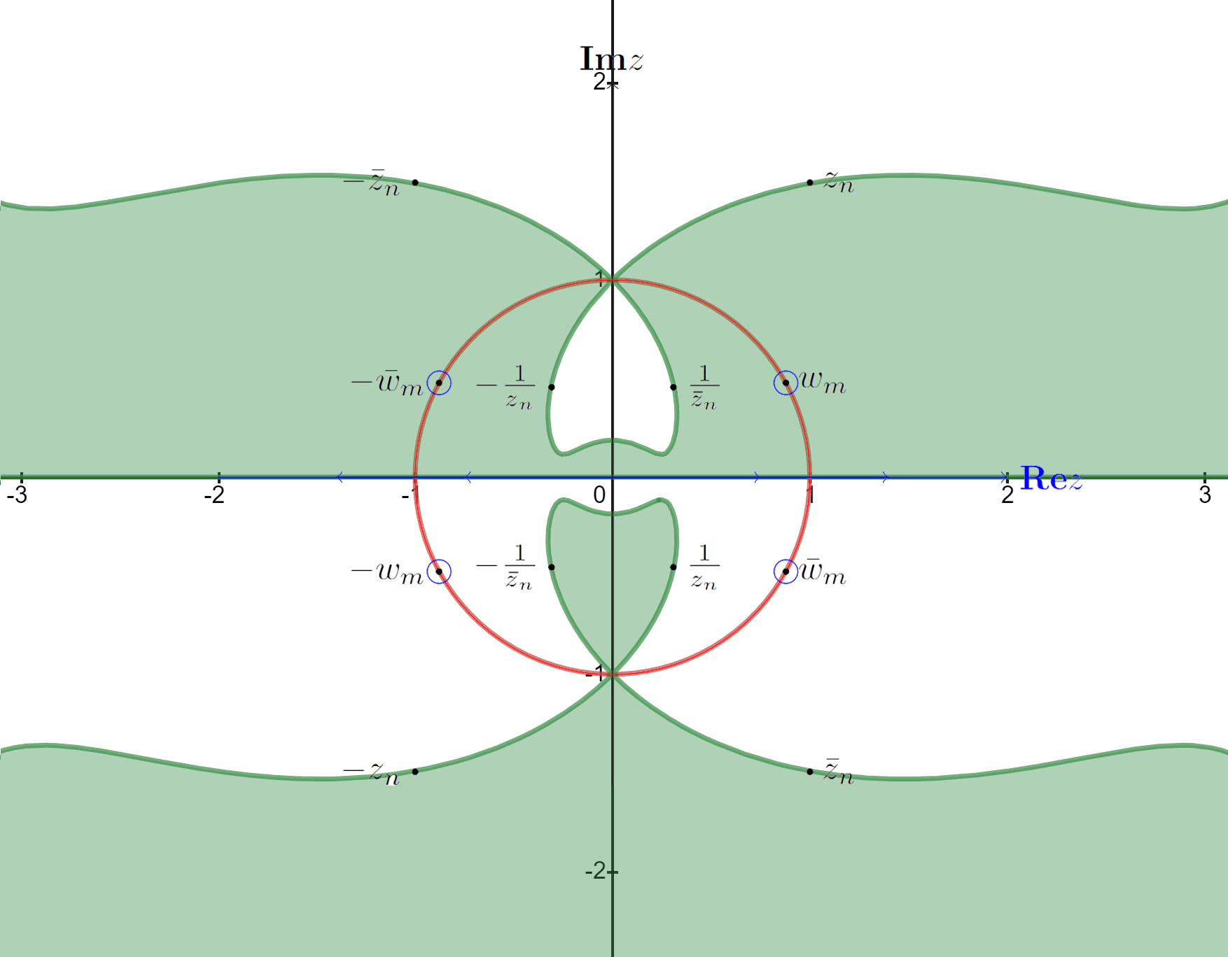
5 Mixed $\bar{\partial}$ -RH Problem

In this section, we make continuous extension to the jump matrix $V^{1}$ to remove the jump from $\mathbb{R}$ . Besides, the new problem is hoped to takes advantage of the decay/growth of $e^{2it\theta(z)}$ for $z\notin\mathbb{R}$ . For this purpose, we introduce some new regions and contours relyed on $\xi$ :

1. for the case $\xi<-\frac{1}{4}$ and $\xi>2$ ,

		$\displaystyle\Omega_{2n+1}=\left\{z\in\mathbb{C}\|n\pi\leq\arg z\leq n\pi+\varphi\right\},$		(5.1)
		$\displaystyle\Omega_{2n+2}=\left\{z\in\mathbb{C}\|(n+1)\pi-\varphi\leq\arg z\leq(n+1)\pi\right\},$		(5.2)

where $n=0,1$ . And

		$\displaystyle\Sigma_{k}=e^{(k-1)i\pi/2+i\varphi}R_{+},\hskip 14.22636ptk=1,3,$		(5.3)
		$\displaystyle\Sigma_{k}=e^{ki\pi/2-i\varphi}R_{+},\hskip 14.22636ptk=2,4,$		(5.4)

which is the boundary of $\Omega_{k}$ respectively. In addition, for these cases, let

		$\displaystyle\Omega(\xi)=\underset{k=1,...,4}{\cup}\Omega_{k},$		(5.5)
		$\displaystyle\Sigma^{(2)}(\xi)=\underset{n\in\mathcal{N}\setminus\Lambda}{\cup}\left(\partial\overline{\mathbb{D}}_{n}\cup\partial\mathbb{D}_{n}\right),\ \tilde{\Sigma}(\xi)=\Sigma_{1}\cup\Sigma_{2}\cup\Sigma_{3}\cup\Sigma_{4},$		(5.6)

which are shown in Figure 6. And $\frac{\pi}{8}>\varphi>0$ is an fixed sufficiently small angle achieving following conditions:
a. $\cos 2\varphi>\frac{4}{\xi}-1$ for $\xi>2$ ;
b. $\cos 2\varphi>-\frac{1}{2\xi}-1$ for $\xi<-\frac{1}{4}$ ;
c. each $\Omega_{i}$ doesn’t intersect $\left\{z\in\mathbb{C}|\text{Im }\theta(z)=0\right\}$ and any of $\mathbb{D}_{n}$ or $\overline{\mathbb{D}}_{n}$ .

2. for the case $-\frac{1}{4}<\xi<2$ , $l\in(0,\frac{|\xi_{j+(-1)^{j}}-\xi_{j}|}{2\cos\varphi})$

		$\displaystyle\Sigma_{jk}(\xi)=\left\{\begin{array}[]{lll}\xi_{j}+e^{i[(k/2+1/2+j)\pi+(-1)^{j+1}\varphi]}l,&\ 0>\xi>-0.25\\ \xi_{j}+e^{i[(k/2+j)\pi+(-1)^{j}\varphi]}l,&\ 0\leq\xi<2\end{array}\right.,\hskip 5.69046ptk=1,3,$
		$\displaystyle\Sigma_{jk}(\xi)=\left\{\begin{array}[]{lll}\xi_{j}+e^{i[(k/2+j)\pi+(-1)^{j}\varphi]}l,&\ 0>\xi>-0.25\\ \xi_{j}+e^{i[(k/2+1/2+j)\pi+(-1)^{j+1}\varphi]}l,&\ 0\leq\xi<2\end{array}\right.,\hskip 5.69046ptk=2,4,$

where $j=2,...,n(\xi)-1$ and for $j=1,n(\xi)$

		$\displaystyle\Sigma_{j1}(\xi)=\left\{\begin{array}[]{lll}\xi_{j}+e^{(1+j)\pi i+(-1)^{j+1}i\varphi}\mathbb{R}^{+},&\ 0>\xi>-0.25\\ \xi_{j}+e^{j\pi i+(-1)^{j}i\varphi}l,&\ 0\leq\xi<2\end{array}\right.,$
		$\displaystyle\Sigma_{j2}(\xi)=\left\{\begin{array}[]{lll}\xi_{j}+e^{(1+j)\pi i+(-1)^{j}i\varphi}\mathbb{R}^{+},&\ 0>\xi>-0.25\\ \xi_{j}+e^{j\pi i+(-1)^{j+1}i\varphi}l,&\ 0\leq\xi<2\end{array}\right.,$
		$\displaystyle\Sigma_{j3}(\xi)=\left\{\begin{array}[]{lll}\xi_{j}+e^{j\pi i+(-1)^{j+1}i\varphi}l,&\ 0>\xi>-0.25\\ \xi_{j}+e^{(1+j)\pi i+(-1)^{j}i\varphi}\mathbb{R}^{+},&\ 0\leq\xi<2\end{array}\right.,$
		$\displaystyle\Sigma_{j4}(\xi)=\left\{\begin{array}[]{lll}\xi_{j}+e^{j\pi i+(-1)^{j}i\varphi}l,&\ 0>\xi>-0.25\\ \xi_{j}+e^{(1+j)\pi i+(-1)^{j+1}i\varphi}\mathbb{R}^{+},&\ 0\leq\xi<2\end{array}\right..$

Moreover, for $l\in(0,\frac{|\xi_{j+(-1)^{j}}-\xi_{j}|}{2\cos\varphi})$ ,

\displaystyle\Sigma_{j\pm}^{\prime}=\left\{\begin{array}[]{lll}\frac{\xi_{j+1}+\xi_{j}}{2}+e^{i\pi}l,&\ 0>\xi>-0.25,\ j=1,...,n(\xi)-1\\ \frac{\xi_{j-1}+\xi_{j}}{2}-e^{i\pi}l,&\ 0\leq\xi<2,\ j=2,...,n(\xi)\end{array}\right..

For convenience, denote $\Sigma_{n(\xi)\pm}^{\prime}=\emptyset$ when $0>\xi>-0.25$ and $\Sigma_{1\pm}^{\prime}=\emptyset$ when $0\leq\xi<2$ . And $\frac{\pi}{8}>\varphi>0$ is an fixed sufficiently small angle achieving following conditions:
1. each $\Omega_{i}$ doesn’t intersect $\left\{z\in\mathbb{C};\text{Im }\theta(z)=0\right\}$ and any of $\mathbb{D}_{n}$ or $\overline{\mathbb{D}}_{n}$ ,
2. $2\tan\varphi>\xi_{n(\xi)/2}-\xi_{n(\xi)/2+1}$ .
This contours separate complex plane $\mathbb{C}$ into sectors shown in Figure 5.

Figure 5: Figure (a) and (b) are corresponding to the

0\leq\xi<2

and

-\frac{1}{4}<\xi<0

respectively.

\Sigma_{ij}

separate complex plane

\mathbb{C}

into some sectors denoted by

\Omega_{ij}

In addition, for these two cases, let

		$\displaystyle\Omega(\xi)=\underset{j=1,..,n(\xi)}{\underset{k=1,...,4,}{\cup}}\Omega_{jk},\hskip 14.22636pt\Omega_{\pm}(\xi)=\mathbb{C}\setminus\Omega,$		(5.21)
		$\displaystyle\tilde{\Sigma}(\xi)=\left(\underset{j=1,..,n(\xi)}{\underset{k=1,...,4,}{\cup}}\Sigma_{jk}\right)\cup\left(\underset{j=1,...,n(\xi)}{\cup}\Sigma^{\prime}{j\pm}\right),\hskip 14.22636pt$		(5.22)
		$\displaystyle\Sigma^{(2)}(\xi)=\tilde{\Sigma}(\xi)\underset{n\in\mathcal{N}\setminus\Lambda}{\cup}\left(\partial\overline{\mathbb{D}}_{n}\cup\partial\mathbb{D}_{n}\right).$		(5.23)

Figure 6: The yellow region is

\Omega(\xi)

. The blue circle around poles not on

\left\{z\in\mathbb{C}|\text{Im }\theta(z)=0\right\}

(here take

z_{n}

as an example) constitute

\Sigma^{(2)}(\xi)

together.

Lemma 7.

Set $\xi=\frac{y}{t}\in(-\infty,-0.25)\cup(2,+\infty)$ . And $f(x)=x+\frac{1}{x}$ is a real-valued function for $x\in\mathbb{R}$ . Then the imaginary part of phase function (4.1) $\text{Im }\theta(z)$ have following estimation:

Case I: for $\xi=\frac{y}{t}\in(2,+\infty)$ ,

		$\displaystyle\text{Im }\theta(z)\geq\|\sin\varphi\|f(l)\left(\frac{\xi}{4}-\frac{1}{\cos 2\varphi+1}\right),\hskip 14.22636pt\text{as }z\in\Omega_{3},\Omega_{4};$		(5.24)
		$\displaystyle\text{Im }\theta(z)\leq-\|\sin\varphi\|f(l)\left(\frac{\xi}{4}-\frac{1}{\cos 2\varphi+1}\right),\hskip 14.22636pt\text{as }z\in\Omega_{1},\Omega_{2}.$		(5.25)

Case IV: for $\xi=\frac{y}{t}\in(-\infty,-0.25)$ ,

		$\displaystyle\text{Im }\theta(z)\geq\|\sin\varphi\|f(l)\left(-\frac{\xi}{4}-\frac{1}{8(\cos 2\varphi+1)}\right),\hskip 14.22636pt\text{as }z\in\Omega_{1},\Omega_{2};$		(5.26)
		$\displaystyle\text{Im }\theta(z)\leq-\|\sin\varphi\|f(l)\left(-\frac{\xi}{4}-\frac{1}{8(\cos 2\varphi+1)}\right),\hskip 14.22636pt\text{as }z\in\Omega_{3},\Omega_{4}.$		(5.27)

Proof.

We take $z\in\Omega_{1}$ as an example, and the other regions are similarly. From (4.1), for $z=le^{i\phi}$ , rewrite $\text{Im }\theta(z)$ as

\displaystyle\text{Im }\theta(z)=f(l)\sin\phi\left(-\frac{\xi}{4}+2\frac{2\cos 2\phi+6-f(l)^{2}}{\left(f(l)^{2}+2\cos 2\phi-2\right)^{2}}\right).

(5.28)

Denote

\displaystyle h(x;a)=\frac{2a+6-x}{\left(x+2a-2\right)^{2}},

(5.29)

with $x\geq 4$ and $0<a\leq 1$ . Then

\displaystyle\frac{\partial h}{\partial x}=\frac{x-(6a+10)}{\left(x+2a-2\right)^{3}}.

(5.30)

So $h(x;a)$ has minimum value

\displaystyle h(6a+10;a)=-\frac{1}{8(a+1)}.

(5.31)

Together with

\displaystyle h(4;a)=\frac{1}{2(a+1)},\hskip 14.22636pt\lim_{x\to+\infty}h(x;a)=0,

(5.32)

we have that $h(x;a)\in\left(-\frac{1}{8(a+1)},\frac{1}{2(a+1)}\right)$ . Then the result is obtained. ∎

Corollary 1.

Set $\xi=\frac{y}{t}\in(-\infty,-0.25)\cup(2,+\infty)$ . There exist a constant $c(\xi)>0$ relied on $\xi$ that the imaginary part of phase function (4.1) $\text{Im }\theta(z)$ have following evaluation for $z=le^{i\phi}=u+vi$ :

Case I: for $\xi=\frac{y}{t}\in(2,+\infty)$ ,

		$\displaystyle\text{Im }\theta(z)\geq c(\xi)v,\hskip 14.22636pt\text{as }z\in\Omega_{3},\Omega_{4};$		(5.33)
		$\displaystyle\text{Im }\theta(z)\leq-c(\xi)v,\hskip 14.22636pt\text{as }z\in\Omega_{1},\Omega_{2}.$		(5.34)

Case IV: for $\xi=\frac{y}{t}\in(-\infty,-0.25)$

		$\displaystyle\text{Im }\theta(z)\geq c(\xi)v,\hskip 14.22636pt\text{as }z\in\Omega_{1},\Omega_{2};$		(5.35)
		$\displaystyle\text{Im }\theta(z)\leq-c(\xi)v,\hskip 14.22636pt\text{as }z\in\Omega_{3},\Omega_{4}.$		(5.36)

Lemma 8.

There exist a constant $c(\xi)>0$ relied on $\xi=\frac{y}{t}\in(-0.25,2)$ that the imaginary part of phase function (4.1) $\text{Im }\theta(z)$ have following estimation for $i=1,...,n(\xi)$ :

		$\displaystyle\text{Im }\theta(z)\geq c(\xi)\text{Im}z\frac{\|z\|^{2}-\xi_{i}^{2}}{4+\|z\|^{2}},\hskip 14.22636pt\text{as }z\in\Omega_{i1},\Omega_{i3};$		(5.37)
		$\displaystyle\text{Im }\theta(z)\leq-c(\xi)\text{Im}z\frac{\|z\|^{2}-\xi_{i}^{2}}{4+\|z\|^{2}},\hskip 14.22636pt\text{as }z\in\Omega_{i2},\Omega_{i4}.$		(5.38)

Proof.

We only give the detail of Case III( $\xi=\frac{y}{t}\in(-0.25,0)$ ) and take $z\in\Omega_{11}$ as an example, and the other regions are similarly. Denote $z=u+\xi_{1}+vi$ with $u,v\in\mathbb{R}$ and

\displaystyle k=-\frac{1}{4}\left(z-\frac{1}{z}\right),\hskip 14.22636ptk_{1}=-\frac{1}{4}\left(\xi_{1}-\frac{1}{\xi_{1}}\right).

(5.39)

Take notice of that $\xi_{1}>1$ , so $k_{1}<1$ . Moreover,

\displaystyle\xi=2\frac{1-4k_{1}^{2}}{(1+4k_{1}^{2})^{2}}<0.

(5.40)

And denote

		$\displaystyle x\triangleq\text{Re}(k-k_{1})=-\frac{1}{4}\left[u+\frac{u^{2}+2\xi_{1}u+v^{2}}{\xi_{1}^{2}[(u+\xi_{1})^{2}+v^{2}]}\right],$		(5.41)
		$\displaystyle y\triangleq\text{Im}(k-k_{1})=-\frac{1}{4}v\left(1+\frac{1}{\|z\|^{2}}\right).$		(5.42)

Then the imaginary part of phase function (4.1) $\text{Im }\theta(z)$ can be rewrite as

\displaystyle\text{Im }\theta(z)=y\left[\xi-2\frac{1-4|k|^{2}}{|1+4k^{2}|^{2}}\right].

(5.43)

Obviously, a simple calculation gives that $\frac{1-4|k|^{2}}{|1+4k^{2}|^{2}}$ is a monotone increasing function of $y$ , so

\displaystyle\text{Im }\theta(z)\geq y\left[\xi-2\frac{1-4(x+k_{1})^{2}}{(1+4(x+k_{1})^{2})^{2}}\right].

(5.44)

Substitute (5.40) into $\xi-2\frac{1-4(x+k_{1})^{2}}{(1+4(x+k_{1})^{2})^{2}}$ and obtained

\displaystyle\xi-2\frac{1-4(x+k_{1})^{2}}{(1+4(x+k_{1})^{2})^{2}}=8\left[(x+k_{1})^{2}-k_{1}^{2}\right]\frac{3-16k_{1}^{2}(x+k_{1})^{2}+4(k_{1}^{2}+(x+k_{1})^{2})}{\left[1+4(x+k_{1})^{2}\right]^{2}(1+4k_{1}^{2})^{2}}

(5.45)

In the product above, the last item has nonzero upper and lower bound for $x\geq 0$ , so

	$\displaystyle\text{Im }\theta(z)$	$\displaystyle\gtrsim v\left(1+\frac{1}{\|z\|^{2}}\right)\frac{(x+k_{1})^{2}-k_{1}^{2}}{1+4(x+k_{1})^{2}}$
		$\displaystyle\gtrsim v\frac{\|z\|^{2}-\xi_{1}^{2}}{1+4\|k\|^{2}}\gtrsim v\frac{\|z\|^{2}-\xi_{1}^{2}}{4+\|z\|^{2}}.$		(5.46)

∎

For Case I and Case VI, introduce following functions for brief:

		$\displaystyle p_{1}(z,\xi)=p_{2}(z,\xi)=\left\{\begin{array}[]{lll}-\dfrac{\bar{r}(z)}{1+\|r(z)\|^{2}},\text{ for }\xi<-0.25\\ -r(z),\text{ for }\xi>2\end{array}\right.,$
		$\displaystyle p_{3}(z,\xi)=p_{4}(z,\xi)=\left\{\begin{array}[]{lll}\dfrac{r(z)}{1+\|r(z)\|^{2}},\text{ for }\xi<-0.25\\ \bar{r}(z),\text{ for }\xi>2\end{array}\right..$

As in Case II and Case III, for $j=1,...,n(\xi)$ ,

		$\displaystyle p_{j1}(z,\xi)=-\dfrac{\bar{r}(z)}{1+\|r(z)\|^{2}},\hskip 14.22636ptp_{j3}(z,\xi)=-r(z),$		(5.51)
		$\displaystyle p_{j2}(z,\xi)=\dfrac{r(z)}{1+\|r(z)\|^{2}},\hskip 17.07182ptp_{j4}(z,\xi)=\bar{r}(z).$		(5.52)

Besides, from $r\in W^{2,2}(\mathbb{R})$ , it also has that $p_{1}^{\prime}(z)$ and $p_{3}^{\prime}(z)$ exist and are in $L^{2}(\mathbb{R})\cup L^{\infty}(\mathbb{R})$ . And $\parallel p_{1}^{\prime}(z)\parallel_{p}\lesssim\parallel r^{\prime}(z)\parallel_{p}$ for $p=2,\infty$ . Then the next step is to construct a matrix function $R^{(2)}$ . We need to remove jump on $\mathbb{R}$ and $i\mathbb{R}$ , and have some mild control on $\bar{\partial}R^{(2)}$ sufficient to ensure that the $\bar{\partial}$ -contribution to the long-time asymptotics of $q(x,t)$ is negligible. Note that $\theta(z)$ has different property in different cases, so the construction of $R^{(2)}(z)$ depend on $x\xi$ . Then we choose $R^{(2)}(z,\xi)$ as:

Case I: for $\xi=\frac{y}{t}\in(2,+\infty)$ ,

R^{(2)}(z,\xi)=\left\{\begin{array}[]{lll}\left(\begin{array}[]{cc}1&0\\ R_{j}(z,\xi)e^{-2it\theta}&1\end{array}\right),&z\in\Omega_{j},j=1,2;\\ \\ \left(\begin{array}[]{cc}1&R_{j}(z,\xi)e^{2it\theta}\\ 0&1\end{array}\right),&z\in\Omega_{j},j=3,4;\\ \\ I,&elsewhere;\\ \end{array}\right.

(5.53)

Case VI: for $\xi=\frac{y}{t}\in(-\infty,-0.25)$ ,

R^{(2)}(z,\xi)=\left\{\begin{array}[]{lll}\left(\begin{array}[]{cc}1&R_{j}(z,\xi)e^{2it\theta}\\ 0&1\end{array}\right),&z\in\Omega_{j},j=1,2;\\ \\ \left(\begin{array}[]{cc}1&0\\ R_{j}(z,\xi)e^{-2it\theta}&1\end{array}\right),&z\in\Omega_{j},j=3,4;\\ \\ I,&elsewhere;\\ \end{array}\right.

(5.54)

where the functions $R_{j}$ , $j=1,2,..,8$ , is defined in following Proposition.

Proposition 6.

$R_{j}$ : $\bar{\Omega}_{j}\to C$ , $j=1,2,..,8$ have boundary values as follow:

Case I: for $\xi=\frac{y}{t}\in(-\infty,-0.25)$ ,

		$\displaystyle R_{1}(z,\xi)=\Bigg\{\begin{array}[]{ll}p_{1}(z,\xi)T_{+}(z)^{-2}&z\in\mathbb{R}^{+},\\ 0&z\in\Sigma_{1},\\ \end{array},\hskip 17.07182ptR_{2}(z,\xi)=\Bigg\{\begin{array}[]{ll}0&z\in\Sigma_{2},\\ p_{2}(z,\xi)T_{+}(z)^{-2}&z\in\mathbb{R}^{-},\\ \end{array}$
		$\displaystyle R_{3}(z,\xi)=\Bigg\{\begin{array}[]{ll}p_{3}(z,\xi)T_{-}(z)^{2}&z\in\mathbb{R}^{-},\\ 0&z\in\Sigma_{3},\\ \end{array},\hskip 17.07182ptR_{4}(z,\xi)=\Bigg\{\begin{array}[]{ll}0&z\in\Sigma_{4},\\ p_{4}(z,\xi)T_{-}(z)^{2}&z\in\mathbb{R}^{+},\\ \end{array}.$

Case II: for $\xi=\frac{y}{t}\in(2,+\infty)$ ,

		$\displaystyle R_{1}(z,\xi)=\Bigg\{\begin{array}[]{ll}p_{1}(z,\xi)T(z)^{2}&z\in\mathbb{R}^{+},\\ 0&z\in\Sigma_{1},\\ \end{array},\hskip 17.07182ptR_{2}(z,\xi)=\Bigg\{\begin{array}[]{ll}0&z\in\Sigma_{2},\\ p_{2}(z,\xi)T(z)^{2}&z\in\mathbb{R}^{-},\\ \end{array}$
		$\displaystyle R_{3}(z,\xi)=\Bigg\{\begin{array}[]{ll}p_{3}(z,\xi)T(z)^{-2}&z\in\mathbb{R}^{-},\\ 0&z\in\Sigma_{3},\\ \end{array},\hskip 17.07182ptR_{4}(z,\xi)=\Bigg\{\begin{array}[]{ll}0&z\in\Sigma_{4},\\ p_{4}(z,\xi)T(z)^{-2}&z\in\mathbb{R}^{+},\\ \end{array}.$

And $R_{j}$ have following property: for $j=1,2,3,4,$

\displaystyle|\bar{\partial}R_{j}(z)|\lesssim|p_{j}^{\prime}(|z|)|+|z|^{-1/2},\text{for all $z\in\Omega_{j}$,}

(5.71)

moreover

\displaystyle|\bar{\partial}R_{j}(z)|\lesssim|p_{j}^{\prime}(|z|)|+|z|^{-1},\text{for all $z\in\Omega_{j}$.}

(5.72)

And

\bar{\partial}R_{j}(z)=0,\hskip 14.22636pt\text{if }z\in elsewhere.

(5.73)

Proof.

For brief, we only proof case I. Taking $R_{1}(z)$ as an example, its extensions can be constructed by:

R_{1}(z)=p_{1}(|z|)T^{-2}(z)\cos(k_{0}\arg z),\hskip 14.22636ptk_{0}=\frac{\pi}{2\varphi}.

(5.74)

The other cases are easily inferred. Denote $z=le^{i\phi}$ , then we have $\bar{\partial}=\frac{e^{i\phi}}{2}\left(\partial_{r}+\frac{i}{r}\partial_{\phi}\right)$ . So

\displaystyle\bar{\partial}R_{1}(z)=\frac{e^{i\phi}}{2}T^{2}(z)\left(p_{1}^{\prime}(r)\cos(k_{0}\phi)-\frac{i}{l}p_{1}(l)k_{0}\sin(k_{0}\phi)\right).

(5.75)

There are two way to bound second term. First we use Cauchy-Schwarz inequality and obtain

|p_{1}(l)|=|p_{1}(l)-p_{1}(0)|=|\int_{0}^{l}p_{1}^{\prime}(s)ds|\leq\parallel p_{1}^{\prime}(s)\parallel_{L^{2}}l^{1/2}\lesssim l^{1/2}.

(5.76)

And note that $T(z)$ is a bounded function in $\bar{\Omega}_{1}$ . Then the boundedness of (5.71) follows immediately. On the side, $p_{1}(l)\in L^{\infty}$ , which implies (5.72). ∎

As in Case II( $\xi=\frac{y}{t}\in[0,2)$ ) and Case III( $\xi=\frac{y}{t}\in(-0.25,0)$ ),

R^{(2)}(z,\xi)=\left\{\begin{array}[]{lll}\left(\begin{array}[]{cc}1&R_{kj}(z,\xi)e^{2it\theta}\\ 0&1\end{array}\right),&z\in\Omega_{kj},j=1,3,\ k=1,...,n(\xi);\\ \\ \left(\begin{array}[]{cc}1&0\\ R_{kj}(z,\xi)e^{-2it\theta}&1\end{array}\right),&z\in\Omega_{kj},j=2,4\ k=1,...,n(\xi);\\ \\ I,&elsewhere;\\ \end{array}\right.

(5.77)

where the functions $R_{kj}$ , $j=1,2,3,4$ , $k=1,...,n(\xi)$ are defined in following Proposition.

Proposition 7.

As in Case II( $\xi=\frac{y}{t}\in[0,2)$ ) and Case III( $\xi=\frac{y}{t}\in(-0.25,0)$ ), the functions $R_{kj}$ : $\bar{\Omega}_{kj}\to\mathbb{C}$ , $j=1,2,3,4$ , $k=1,...,n(\xi)$ have boundary values as follow:

		$\displaystyle R_{k1}(z,\xi)=\Bigg\{\begin{array}[]{ll}p_{k1}(z,\xi)T_{+}(z)^{-2}&z\in I_{k1},\\ p_{k1}(\xi_{k},\xi)T_{k}(\xi)^{-2}(z-\xi_{k})^{-2i\nu(\xi_{k})}&z\in\Sigma_{k1},\\ \end{array},$
		$\displaystyle R_{k2}(z,\xi)=\Bigg\{\begin{array}[]{ll}p_{k2}(\xi_{k},\xi)T_{k}(\xi)^{2}(z-\xi_{k})^{2i\nu(\xi_{k})}&z\in\Sigma_{k2},\\ p_{k2}(z,\xi)T_{-}(z)^{2}&z\in I_{k2},\\ \end{array}$
		$\displaystyle R_{k3}(z,\xi)=\Bigg\{\begin{array}[]{ll}p_{k3}(z,\xi)T(z)^{-2}&z\in I_{k3},\\ p_{k3}(\xi_{k},\xi)T_{k}(\xi)^{-2}(z-\xi_{k})^{-2i\nu(\xi_{k})}&z\in\Sigma_{k3},\\ \end{array}$
		$\displaystyle R_{k4}(z,\xi)=\Bigg\{\begin{array}[]{ll}p_{k4}(\xi_{k},\xi)T_{k}(\xi)^{2}(z-\xi_{k})^{2i\nu(\xi_{k})}&z\in\Sigma_{k4},\\ p_{k4}(z,\xi)T(z)^{2}&z\in I_{k4},\\ \end{array},$

where $I_{kj}$ is specified in (4)-(4). And $R_{kj}$ have following property:

		$\displaystyle\|R_{kj}(z,\xi)\|\lesssim\sin^{2}(k_{0}\arg(z-\xi_{k}))+\left(1+\text{Re}(z)^{2}\right)^{-1/2},\text{for all $z\in\Omega_{kj}$},$		(5.86)
		$\displaystyle\|\bar{\partial}R_{kj}(z,\xi)\|\lesssim\|p_{kj}^{\prime}(\text{Re}z)\|+\|z-\xi_{k}\|^{-1/2},\text{for all $z\in\Omega_{kj}$.}$		(5.87)

And

\bar{\partial}R_{kj}(z,\xi)=0,\hskip 14.22636pt\text{if }z\in elsewhere.

(5.88)

Proof.

We give the details for $R_{11}$ only. The other cases are easily inferred. Using the constants $T_{k}(\xi)$ defined in proposition 5, give the extension of $R_{11}(z,\xi)$ on $\Omega_{11}$ :

	$\displaystyle R_{11}(z,\xi)=$	$\displaystyle p_{11}(\xi_{1},\xi)T_{1}(\xi)^{-2}(z-\xi_{1})^{-2i\nu(\xi_{1})}\left[1-\cos\big(k_{0}\arg(z-\xi_{1})\big)\right]$		(5.89)
		$\displaystyle+\cos\big(k_{0}\arg(z-\xi_{1})\big)p_{11}(\text{Re}z,\xi)T(z)^{-2}.$		(5.90)

Let $z-\xi_{1}=le^{i\psi}=u+vi$ , $l,\psi,u,v\in\mathbb{R}$ . And from $r\in H^{1,1}(\mathbb{R})$ , which means $p_{11}\in H^{1,1}(R)$ we have $|p_{11}(u)|\lesssim(1+u^{2})^{-1/2}$ . Together with (4.41) we have (5.86). Since

\bar{\partial}=\frac{1}{2}\left(\partial_{u}+i\partial_{v}\right)=\frac{e^{i\psi}}{2}\left(\partial_{l}+il^{-1}\partial_{\psi}\right),

we have

	$\displaystyle\bar{\partial}R_{11}$	$\displaystyle=\left(p_{11}(u,\xi)T(z)^{-2}-p_{11}(\xi_{1},\xi)T_{1}(\xi)^{-2}(z-\xi_{1})^{-2i\nu(\xi_{1})}\right)\bar{\partial}\cos(k_{0}\psi)$		(5.91)
		$\displaystyle+\frac{1}{2}T(z)^{-2}p_{11}^{\prime}(u,\xi)\cos(k_{0}\psi).$		(5.92)

Substitute (4.37) into above equation, (5.87) comes immediately. ∎

In addition, from Proposition 1, $R^{(2)}$ achieve the symmetry:

R^{(2)}(z)=\sigma_{3}\overline{R^{(2)}(-\bar{z})}\sigma_{3}=\overline{R^{(2)}(-1/\bar{z})}=\sigma_{3}R^{(2)}(-1/z)\sigma_{3}.

(5.93)

We now use $R^{(2)}$ to define the new transformation

M^{(2)}(z;y,t)\triangleq M^{(2)}(z)=M^{(1)}(z)R^{(2)}(z),

(5.94)

which satisfies the following mixed $\bar{\partial}$ -RH problem.

RHP 4.

Find a matrix valued function $M^{(2)}(z)$ with following properties:

$\blacktriangleright$ Analyticity: $M^{(2)}(z)$ is continuous in $\mathbb{C}$ , sectionally continuous first partial derivatives in $\mathbb{C}\setminus\left(\Sigma^{(2)}\cup\left\{\zeta_{n},\bar{\zeta}_{n}\right\}_{n\in\Lambda}\right)$ and meromorphic out $\bar{\Omega}$ ;

$\blacktriangleright$ Symmetry: $M^{(2)}(z)=\sigma_{3}\overline{M^{(2)}(-\bar{z})}\sigma_{3}$ = $F^{-2}\overline{M^{(2)}(-\bar{z}^{-1})}$ = $F^{2}\sigma_{3}M^{(2)}(-z^{-1})\sigma_{3}$ ;

$\blacktriangleright$ Jump condition: $M^{(2)}$ has continuous boundary values $M^{(2)}_{\pm}$ on $\Sigma^{(2)}$ and

M^{(2)}_{+}(z)=M^{(2)}_{-}(z)V^{(2)}(z),\hskip 14.22636ptz\in\Sigma^{(2)},

(5.95)

where for $\xi=\frac{y}{t}\in(2,+\infty)$ or $\xi=\frac{y}{t}\in(-\infty,-0.25)$

V^{(2)}(z)=\left\{\begin{array}[]{ll}\left(\begin{array}[]{cc}1&0\\ -C_{n}(z-\zeta_{n})^{-1}T^{2}(z)e^{-2it\theta_{n}}&1\end{array}\right),&\text{as }z\in\partial\mathbb{D}_{n},n\in\nabla;\\[12.0pt] \left(\begin{array}[]{cc}1&-C_{n}^{-1}(z-\zeta_{n})T^{-2}(z)e^{2it\theta_{n}}\\ 0&1\end{array}\right),&\text{as }z\in\partial\mathbb{D}_{n},n\in\Delta;\\ \left(\begin{array}[]{cc}1&\bar{C}_{n}(z-\bar{\zeta}_{n})^{-1}T^{-2}(z)e^{2it\bar{\theta}_{n}}\\ 0&1\end{array}\right),&\text{as }z\in\partial\overline{\mathbb{D}}_{n},n\in\nabla;\\ \left(\begin{array}[]{cc}1&0\\ \bar{C}_{n}^{-1}(z-\bar{\zeta}_{n})e^{-2it\bar{\theta}_{n}}T^{2}(z)&1\end{array}\right),&\text{as }z\in\partial\overline{\mathbb{D}}_{n},n\in\Delta;\\ \end{array}\right.,

(5.96)

and for $\xi=\frac{y}{t}\in(-0.25,2)$

V^{(2)}(z)=\left\{\begin{array}[]{ll}R^{(2)}(z)|_{\Sigma_{k1}\cup\Sigma_{k4}}&\text{as }z\in\Sigma_{k1}\cup\Sigma_{k4};\\[12.0pt] R^{(2)}(z)^{-1}|_{\Sigma_{k2}\cup\Sigma_{k3}}&\text{as }z\in\Sigma_{k2}\cup\Sigma_{k3};\\[12.0pt] R^{(2)}(z)^{-1}|_{\Sigma_{k\ (3\pm 1)/2}}R^{(2)}(z)|_{\Sigma_{(k-1)\ (3\pm 1)/2}}&\text{as }z\in\Sigma_{k\pm}^{\prime},\ k\text{ is even};\\[12.0pt] R^{(2)}(z)^{-1}|_{\Sigma_{k\ (7\pm 1)/2}}R^{(2)}(z)|_{\Sigma_{(k-1)\ (7\pm 1)/2}}&\text{as }z\in\Sigma_{k\pm}^{\prime},\ k\text{ is odd};\\[12.0pt] \left(\begin{array}[]{cc}1&0\\ -C_{n}(z-\zeta_{n})^{-1}T^{2}(z)e^{-2it\theta_{n}}&1\end{array}\right),&\text{as }z\in\partial\mathbb{D}_{n},n\in\nabla;\\[12.0pt] \left(\begin{array}[]{cc}1&-C_{n}^{-1}(z-\zeta_{n})T^{-2}(z)e^{2it\theta_{n}}\\ 0&1\end{array}\right),&\text{as }z\in\partial\mathbb{D}_{n},n\in\Delta;\\ \left(\begin{array}[]{cc}1&\bar{C}_{n}(z-\bar{\zeta}_{n})^{-1}T^{-2}(z)e^{2it\bar{\theta}_{n}}\\ 0&1\end{array}\right),&\text{as }z\in\partial\overline{\mathbb{D}}_{n},n\in\nabla;\\ \left(\begin{array}[]{cc}1&0\\ \bar{C}_{n}^{-1}(z-\bar{\zeta}_{n})e^{-2it\bar{\theta}_{n}}T^{2}(z)&1\end{array}\right),&\text{as }z\in\partial\overline{\mathbb{D}}_{n},n\in\Delta;\\ \end{array}\right.;

(5.97)

$\blacktriangleright$ Asymptotic behaviors:

$\displaystyle M^{(2)}(z)=$	$\displaystyle I+\mathcal{O}(z^{-1}),\hskip 14.22636ptz\rightarrow\infty,$	(5.98)
$\displaystyle M^{(2)}(z)=$	$\displaystyle F^{-1}\left[I+(z-i)\left(\begin{array}[]{cc}0&-\frac{1}{2}(u+u_{x})\\ -\frac{1}{2}(u-u_{x})&0\end{array}\right)\right]$
	$\displaystyle e^{\frac{1}{2}c_{+}\sigma_{3}}T(i)^{\sigma_{3}}\big(I-I_{0}\sigma_{3}(z-i)\big)+\mathcal{O}\left((z-i)^{2}\right)+\mathcal{O}\left((z-i)^{2}\right);$	(5.101)

$\blacktriangleright$ $\bar{\partial}$ -Derivative: For $z\in\mathbb{C}$ we have

\displaystyle\bar{\partial}M^{(2)}=M^{(2)}\bar{\partial}R^{(2)},

(5.102)

where Case I: for $\xi=\frac{y}{t}\in(-\infty,-0.25)$

\bar{\partial}R^{(2)}(z,\xi)=\left\{\begin{array}[]{lll}\left(\begin{array}[]{cc}0&\bar{\partial}R_{j}(z,\xi)e^{2it\theta}\\ 0&0\end{array}\right),&z\in\Omega_{j},j=1,2;\\ \\ \left(\begin{array}[]{cc}0&0\\ \bar{\partial}R_{j}(z,\xi)e^{-2it\theta}&0\end{array}\right),&z\in\Omega_{j},j=3,4;\\ \\ 0,&elsewhere;\\ \end{array}\right.

(5.103)

Case II: for $\xi=\frac{y}{t}\in(2,+\infty)$

\bar{\partial}R^{(2)}(z,\xi)=\left\{\begin{array}[]{lll}\left(\begin{array}[]{cc}0&0\\ \bar{\partial}R_{j}(z,\xi)e^{-2it\theta}&0\end{array}\right),&z\in\Omega_{j},j=1,2;\\ \\ \left(\begin{array}[]{cc}0&\bar{\partial}R_{j}(z,\xi)e^{2it\theta}\\ 0&0\end{array}\right),&z\in\Omega_{j},j=3,4;\\ \\ 0,&elsewhere;\\ \end{array}\right.

(5.104)

Case II( $\xi=\frac{y}{t}\in[0,2)$ ) and Case III( $\xi=\frac{y}{t}\in(-0.25,0)$ )

\bar{\partial}R^{(2)}(z,\xi)=\left\{\begin{array}[]{lll}\left(\begin{array}[]{cc}0&0\\ \bar{\partial}R_{kj}(z,\xi)e^{-2it\theta}&0\end{array}\right),&z\in\Omega_{kj},j=1,3,\ k=1,...,n(\xi);\\ \\ \left(\begin{array}[]{cc}0&\bar{\partial}R_{kj}(z,\xi)e^{2it\theta}\\ 0&0\end{array}\right),&z\in\Omega_{kj},j=2,4\ k=1,...,n(\xi);\\ \\ 0,&elsewhere;\\ \end{array}\right.

(5.105)

$\blacktriangleright$ Residue conditions: $M^{(2)}$ has simple poles at each point $\zeta_{n}$ and $\bar{\zeta}_{n}$ for $n\in\Lambda$ with:

		$\displaystyle\res_{z=\zeta_{n}}M^{(2)}(z)=\lim_{z\to\zeta_{n}}M^{(2)}(z)\left(\begin{array}[]{cc}0&0\\ C_{n}e^{-2it\theta_{n}}T^{2}(\zeta_{n})&0\end{array}\right),$
		$\displaystyle\res_{z=\bar{\zeta}_{n}}M^{(2)}(z)=\lim_{z\to\bar{\zeta}_{n}}M^{(2)}(z)\left(\begin{array}[]{cc}0&-\bar{C}_{n}T^{-2}(\bar{\zeta}_{n})e^{2it\bar{\theta}_{n}}\\ 0&0\end{array}\right).$

6 Decomposition of the mixed $\bar{\partial}$ -RH problem

To solve RHP2, we decompose it into a model RH problem for $M^{R}(z;y,t)\triangleq M^{R}(z)$ with $\bar{\partial}R^{(2)}\equiv 0$ and a pure $\bar{\partial}$ -Problem with nonzero $\bar{\partial}$ -derivatives. First we establish a RH problem for the $M^{R}(z)$ as follows.

RHP 5.

Find a matrix-valued function $M^{R}(z)$ with following properties:

$\blacktriangleright$ Analyticity: $M^{R}(z)$ is meromorphic in $\mathbb{C}\setminus\Sigma^{(2)}$ ;

$\blacktriangleright$ Jump condition: $M^{R}$ has continuous boundary values $M^{R}_{\pm}$ on $\Sigma^{(2)}$ and

M^{R}_{+}(z)=M^{R}_{-}(z)V^{(2)}(z),\hskip 14.22636ptz\in\Sigma^{(2)};

(6.1)

$\blacktriangleright$ Symmetry: $M^{R}(z)=\sigma_{3}\overline{M^{R}(-\bar{z})}\sigma_{3}$ = $F^{-2}\overline{M^{R}(-\bar{z}^{-1})}$ = $F^{2}\sigma_{3}M^{R}(-z^{-1})\sigma_{3}$ ;

$\blacktriangleright$ $\bar{\partial}$ -Derivative: $\bar{\partial}R^{(2)}=0$ , for $z\in\mathbb{C}$ ;

$\blacktriangleright$ Asymptotic behaviors:

$\displaystyle M^{R}(z)=$	$\displaystyle I+\mathcal{O}(z^{-1}),\hskip 14.22636ptz\rightarrow\infty,$	(6.2)
$\displaystyle M^{R}(z)=$	$\displaystyle F^{-1}\left[I+(z-i)\left(\begin{array}[]{cc}0&-\frac{1}{2}(u+u_{x})\\ -\frac{1}{2}(u-u_{x})&0\end{array}\right)\right]$
	$\displaystyle e^{\frac{1}{2}c_{+}\sigma_{3}}T(i)^{\sigma_{3}}\big(I-I_{0}\sigma_{3}(z-i)\big)+\mathcal{O}\left((z-i)^{2}\right);$	(6.5)

$\blacktriangleright$ Residue conditions: $M^{R}$ has simple poles at each point $\zeta_{n}$ and $\bar{\zeta}_{n}$ for $n\in\Lambda$ with:

		$\displaystyle\res_{z=\zeta_{n}}M^{R}(z)=\lim_{z\to\zeta_{n}}M^{R}(z)\left(\begin{array}[]{cc}0&0\\ C_{n}e^{-2it\theta_{n}}T^{2}(\zeta_{n})&0\end{array}\right),$
		$\displaystyle\res_{z=\bar{\zeta}_{n}}M^{R}(z)=\lim_{z\to\bar{\zeta}_{n}}M^{R}(z)\left(\begin{array}[]{cc}0&-\bar{C}_{n}T^{-2}(\bar{\zeta}_{n})e^{2it\bar{\theta}_{n}}\\ 0&0\end{array}\right).$

In the case of $\xi=\frac{y}{t}\in(-0.25,2)$ , it can be found that compared with $\xi=\frac{y}{t}\in(2,+\infty)\cup(-\infty,-0.25)$ , its jump matrix $V^{(2)}$ has additional portion on $\Sigma_{jk}$ and $\Sigma_{j\pm}$ . So this case is more difficult to deal with. And denote $U(\xi)$ as the union set of neighborhood of $\xi_{j}$ for $j=1,...,n(\xi)$

U(\xi)=\underset{j=1,...,n(\xi)}{\cup}U_{\xi_{j}},\ U_{\xi_{j}}=\left\{z:|z-\xi_{j}|\leq\min\left\{\varrho,\frac{1}{3}\min_{j\neq i\in\mathcal{N}}|\zeta_{i}-\zeta_{j}|\right\}\right\}.

(6.10)

Then this additional part of jump matrix $V^{(2)}$ has following estimation.

Proposition 8.

As $t\to\infty$ , for $1\leq p\leq+\infty$ , there exist a positive constant $K_{p}$ relied on $p$ satisfies that the jump matrix $V^{(2)}$ defined in (5.97) admits

\displaystyle\parallel V^{(2)}-I\parallel_{L^{p}(\Sigma_{kj}\setminus U(\xi_{k}))}=\mathcal{O}(e^{-K_{p}t}),

(6.11)

for $k=1,...,n(\xi)$ and $j=1,...,4$ . And when $1\leq p<+\infty$ , there also exist a positive constant $K_{p}^{\prime}$ relied on $p$ satisfies that the jump matrix $V^{(2)}$ admits

\displaystyle\parallel V^{(2)}-I\parallel_{L^{p}(\Sigma_{k\pm}^{\prime})}=\mathcal{O}(e^{-K_{p}^{\prime}t}),

(6.13)

for $k=1,...,n(\xi)$ .

Proof.

We prove the case $\xi=\frac{y}{t}\in(-0.25,0)$ , and the another case can be proved in similar way. For $z\in\Sigma_{11}\setminus U_{\xi_{1}}$ , when $1\leq p<+\infty$ , by using definition of $V^{(2)}$ and (5.86), we have

	$\displaystyle\parallel V^{(2)}-I\parallel_{L^{p}(\Sigma_{11}\setminus U_{\xi_{1}})}$	$\displaystyle=\parallel p_{11}(\xi_{1},\xi)T_{1}(\xi)^{-2}(z-\xi_{1})^{-2i\nu(\xi_{1})}e^{2it\theta}\parallel_{L^{p}(\Sigma_{11}\setminus U_{\xi_{1}})}$
		$\displaystyle\lesssim\parallel e^{2it\theta}\parallel_{L^{p}(\Sigma_{11}\setminus U_{\xi_{1}})}.$		(6.15)

For $z\in\Sigma_{11}\setminus U_{\xi_{1}}$ , denote $z=\xi_{1}+le^{i\varphi}$ , $l\in(\varrho,+\infty)$ . Then lemma 8 gives that

	$\displaystyle\parallel V^{(2)}-I\parallel_{L^{p}(\Sigma_{11}\setminus U_{\xi_{1}})}^{p}$	$\displaystyle\lesssim\int_{\Sigma_{11}\setminus U_{\xi_{1}}}\exp\left(-pc(\xi)t\text{Im}z\frac{\|z\|^{2}-\xi_{1}^{2}}{4+\|z\|^{2}}\right)dz$
		$\displaystyle\lesssim\int_{\varrho}^{+\infty}\exp\left(-pc^{\prime}(\xi)tl\right)dl\lesssim t^{-1}\exp\left(-pc^{\prime}(\xi)t\varrho\right).$		(6.16)

The second step is from $\frac{|z|^{2}-\xi_{1}^{2}}{4+|z|^{2}}$ has nonzero boundary on $\Sigma_{11}\setminus U_{\xi_{1}}$ . And when $p=+\infty$ is obviously. For $z\in\Sigma_{k\pm}^{\prime}$ , we only give the details of $\Sigma_{1+}^{\prime}$ . there also has that

	$\displaystyle\parallel V^{(2)}-I\parallel_{L^{p}(\Sigma_{1+}^{\prime})}$	$\displaystyle=\parallel(R_{24}-R_{14})e^{-2it\theta}\parallel_{L^{p}(\Sigma_{1+}^{\prime})}\lesssim\parallel e^{-2it\theta}\parallel_{L^{p}(\Sigma_{1+}^{\prime})}$
		$\displaystyle\lesssim t^{-1/p}\exp\left(-c^{\prime\prime}(\xi)t\right).$		(6.17)

∎

This proposition means that the jump matrix $V^{(2)}(z)$ uniformly goes to $I$ on $\tilde{\Sigma}\setminus U(\xi)$ . So outside the $U(\xi)$ there is only exponentially small error (in $t$ ) by completely ignoring the jump condition of $M^{R}(z)$ . And this proposition enlightens us to construct the solution $M^{R}(z)$ as follow:

M^{R}(z)=\left\{\begin{array}[]{ll}E(z,\xi)M^{(r)}(z)&z\notin U(\xi)\\ E(z,\xi)M^{(r)}(z)M^{lo}(z)&z\in U(\xi)\\ \end{array}\right..

(6.18)

Note that, when $\xi=\frac{y}{t}\in(2,+\infty)$ or $\xi=\frac{y}{t}\in(-\infty,-0.25)$ , $M^{(r)}(z)$ has no jump except the circle around poles not in $\Lambda$ , and it has no phase point. So $U(\xi)=\emptyset$ in these case, which means $M^{R}(z)=M^{(r)}(z)$ . And it is more easy. And for the case $\xi=\frac{y}{t}\in(-0.25,2)$ , from the definition we can easily find that $M^{R}$ is pole free. This construction decomposes $M^{R}$ to two part: $M^{(o)}$ solves the pure RHP obtained by ignoring the jump conditions of RHP 5, which is shown in Section 7; $M^{lo}$ uses parabolic cylinder functions to build a matrix to match jumps of $M^{(2)}$ in a neighborhood of each critical point $\xi_{j}$ which is shown in Section 8. And $E(z,\xi)$ is the error function, which will be different in different case of $\xi$ and is a solution of a small-norm Riemann-Hilbert problem shown in Section 9.

We now use $M^{R}(z)$ to construct a new matrix function

M^{(3)}(z;y,t)\triangleq M^{(3)}(z)=M^{(2)}(z)M^{R}(z)^{-1}.

(6.19)

which removes analytical component $M^{R}$ to get a pure $\bar{\partial}$ -problem.

$\bar{\partial}$ -problem. Find a matrix-valued function $M^{(3)}(z;y,t)\triangleq M^{(3)}(z)$ with following identities:

$\blacktriangleright$ Analyticity: $M^{(3)}(z)$ is continuous and has sectionally continuous first partial derivatives in $\mathbb{C}$ .

$\blacktriangleright$ Asymptotic behavior:

\displaystyle M^{(3)}(z)\sim I+\mathcal{O}(z^{-1}),\hskip 14.22636ptz\rightarrow\infty;

(6.20)

$\blacktriangleright$ $\bar{\partial}$ -Derivative: We have

\bar{\partial}M^{(3)}=M^{(3)}W^{(3)},\ \ z\in\mathbb{C},

where

W^{(3)}=M^{R}(z)\bar{\partial}R^{(2)}(z)M^{R}(z)^{-1}.

(6.21)

Proof.

By using properties of the solutions $M^{(2)}$ and $M^{R}$ for RHP 5 and $\bar{\partial}$ -problem , the analyticity is obtained immediately. Since $M^{(2)}$ and $M^{R}$ achieve same jump matrix, we have

	$\displaystyle M_{-}^{(3)}(z)^{-1}M_{+}^{(3)}(z)$	$\displaystyle=M_{-}^{(2)}(z)^{-1}M_{-}^{R}(z)M_{+}^{R}(z)^{-1}M_{+}^{(2)}(z)$
		$\displaystyle=M_{-}^{(2)}(z)^{-1}V^{(2)}(z)^{-1}M_{+}^{(2)}(z)=I,$

which means $M^{(3)}$ has no jumps and is everywhere continuous. We also can show that $M^{(3)}$ has no pole. For $\lambda\in\left\{\zeta_{n},\bar{\zeta}_{n}\right\}_{n\in\Lambda}$ , let $\mathcal{W}$ denote the nilpotent matrix which appears in the left side of the corresponding residue condition of RHP 4 and RHP 5, we have the Laurent expansions in $z-\lambda$

		$\displaystyle M^{(2)}(z)=a(\lambda)\left[\dfrac{\mathcal{W}}{z-\lambda}+I\right]+\mathcal{O}(z-\lambda),$
		$\displaystyle M^{R}(z)=A(\lambda)\left[\dfrac{\mathcal{W}}{z-\lambda}+I\right]+\mathcal{O}(z-\lambda),$

where $a(\lambda)$ and $A(\lambda)$ are the constant matrix in their respective expansions. Then

	$\displaystyle M^{(3)}(z)$	$\displaystyle=\left\{a(\lambda)\left[\dfrac{\mathcal{W}}{z-\lambda}+I\right]\right\}\left\{\left[\dfrac{-\mathcal{W}}{z-\lambda}+I\right]\sigma_{2}A(\lambda)^{T}\sigma_{2}\right\}+\mathcal{O}(z-\lambda)$
		$\displaystyle=\mathcal{O}(1),$		(6.22)

which implies that $M^{(3)}(z)$ has removable singularities at $\lambda$ . And the $\bar{\partial}$ -derivative of $M^{(3)}(z)$ come from $M^{(3)}(z)$ due to analyticity of $M^{R}(z)$ . ∎

The unique existence and asymptotic of $M^{(3)}(z)$ will shown in section 9.

7 The asymptotic $\mathcal{N}(\Lambda)$ -soliton solution

In this subsection, we build a reflectionless case of RHP 2 to show that its solution can approximated with $M^{(r)}(z)$ . As $W^{(3)}(z)\equiv 0$ , RHP 4 reduces to RHP 5 for the sectionally meromorphic function $M^{(r)}(z)$ with jump discontinuities on the union of circles. Then, by relate $M^{(r)}(z)$ with original Riemann Hilbert problem 2, we show the existence and uniqueness of solution of the above RHP 5.

Proposition 9.

If $M^{(r)}(z)$ is the solution of the RH problem 5 with scattering data $\mathcal{D}=\left\{r(z),\left\{\zeta_{n},C_{n}\right\}_{n\in\mathcal{N}}\right\}$ , $M^{(r)}(z)$ exists unique.

Proof.

To transform $M^{(r)}(z)$ to the soliton-solution of RHP 2, the jumps and poles need to be restored. We reverses the triangularity effected in (4.44) and (5.94):

N(z;\tilde{\mathcal{D}})=\left(\prod_{n\in\Delta}\zeta_{n}\right)^{-\sigma_{3}}M^{(r)}(z)T^{-\hat{\sigma}_{3}}G^{-1}(z)\left(\prod_{n\in\Delta}\dfrac{z-\zeta_{n}}{\bar{\zeta}_{n}^{-1}z-1}\right)^{-\sigma_{3}},

(7.1)

with $G(z)$ defined in (4.43) and $\tilde{\mathcal{D}}=\left\{r(z),\left\{\zeta_{n},C_{n}\delta(\zeta_{n})\right\}_{n\in\mathcal{N}}\right\}$ . First we verify $N(z;\tilde{\mathcal{D}})$ satisfying RHP 2. This transformation to $N(z;\tilde{\mathcal{D}})$ preserves the normalization conditions at the origin and infinity obviously. And comparing with (4.44), this transformation restore the jump on $\overline{\mathbb{D}}_{n}$ and $\mathbb{D}_{n}$ to residue for $n\notin\Lambda$ . As for $n\in\Lambda$ , take $\zeta_{n}$ as an example. Substitute (5) into the transformation:

	$\displaystyle\res_{z=\zeta_{n}}N(z;\tilde{\mathcal{D}})=$	$\displaystyle\left(\prod_{n\in\Delta}\zeta_{n}\right)^{-\sigma_{3}}\res_{z=\zeta_{n}}M^{(r)}(z)T^{-\hat{\sigma}_{3}}G(z)^{-1}\left(\prod_{n\in\Delta}\dfrac{z-\zeta_{n}}{\bar{\zeta}_{n}^{-1}z-1}\right)^{-\sigma_{3}}$
	$\displaystyle=$	$\displaystyle\lim_{z\to\zeta_{n}}-\left(\prod_{n\in\Delta}\zeta_{n}\right)^{-\sigma_{3}}M^{(r)}(z)\left(\begin{array}[]{cc}0&0\\ C_{n}e^{-2it\theta_{n}}T^{2}(\zeta_{n})&0\end{array}\right)\left(\prod_{n\in\Delta}\dfrac{z-\zeta_{n}}{\bar{\zeta}_{n}^{-1}z-1}\right)^{-\sigma_{3}}$
	$\displaystyle=$	$\displaystyle\lim_{z\to\zeta_{n}}N(z;\tilde{\mathcal{D}})\left(\begin{array}[]{cc}0&0\\ C_{n}\delta(\zeta_{n})e^{-2it\theta_{n}}&0\end{array}\right).$

Its analyticity and symmetry follow from the Proposition of $M^{(r)}(z)$ , $T(z)$ and $G(z)$ immediately. Although $N(z;\tilde{\mathcal{D}})$ doesn’t preserve the normalization conditions at $z=i$ as (2), $z=i$ isn’t the pole of $N(z)$ . So it make no difference. Then $N(z;\tilde{\mathcal{D}})$ is solution of RHP 2 with absence of reflection, whose exact solution exists and can be obtained as described similarly in [25] Appendix A. And its uniqueness comes from Liouville’s theorem. Then the uniqueness and existences of $M^{(r)}(z)$ come from (7.1). ∎

Although $M^{(r)}(z)$ has uniqueness and existence, not all discrete spectra have contribution as $t\to\infty$ . Following Lemma give that the jump matrices is uniformly near identity and do not meaningfully, contribute to the asymptotic behavior of the solution.

Lemma 9.

The jump matrix $V^{(2)}(z)$ in (5.96) satisfies

\displaystyle\parallel V^{(2)}(z)-I\parallel_{L^{\infty}(\Sigma^{(2)})}=\mathcal{\mathcal{O}}(e^{-2\rho_{0}t}),\hskip 14.22636pt\text{ with $\rho_{0}$ specified in (\ref{rho0}).}

(7.6)

Proof.

Take $z\in\partial\mathbb{D}_{n},$ $n\in\nabla$ as an example.

$\displaystyle\parallel V^{(2)}(z)-I\parallel_{L^{\infty}(\partial\mathbb{D}_{n})}$	$\displaystyle=\|C_{n}(z-\zeta_{n})^{-1}T^{2}(z)e^{-2it\theta_{n}}\|$
	$\displaystyle\lesssim\varrho^{-1}e^{-\text{Re}(2it\theta_{n})}\lesssim e^{2t\text{Im}(\theta_{n})}$
	$\displaystyle\leq e^{-2\rho_{0}t}.$	(7.7)

The last step follows from that for $n\in\nabla$ , $\text{Im}\theta_{n}<0$ . ∎

Corollary 2.

For $1\leq p\leq+\infty$ , the jump matrix $V^{(2)}(z)$ satisfies

\parallel V^{(2)}(z)-I\parallel_{L^{p}(\Sigma^{(2)})}\leq K_{p}e^{-2\rho_{0}t},

(7.8)

for some constant $K_{p}\geq 0$ depending on $p$ .

This estimation of $V^{(2)}(z)$ inspires us to consider to completely ignore the jump condition on $M^{(r)}(z)$ , because there is only exponentially small error (in t). We decompose $M^{(r)}(z)$ as

M^{(r)}(z)=\tilde{E}(z)M^{(r)}_{\Lambda}(z).

(7.9)

$\tilde{E}(z)$ is a error function, which is a solution of a small-norm RH problem and we will discuss it in next subsection 7.1. And $M^{(r)}_{\Lambda}(z)$ solves RHP 5 with $V^{(2)}(z)\equiv 0$ .

Then the RHP 5 reduces to the following RH problem.

RHP 6.

Find a matrix-valued function $M^{(r)}_{\Lambda}(z)$ with following properties:

$\blacktriangleright$ Analyticity: $M^{(r)}_{\Lambda}(z)$ is analytical in $\mathbb{C}\setminus\left\{\zeta_{n},\bar{\zeta}_{n}\right\}_{n\in\Lambda}$ ;

$\blacktriangleright$ Symmetry: $M^{(r)}_{\Lambda}(z)=\sigma_{3}\overline{M^{(r)}_{\Lambda}(-\bar{z})}\sigma_{3}$ = $F^{-2}\overline{M^{(r)}_{\Lambda}(-\bar{z}^{-1})}$ = $F^{2}\sigma_{3}M^{(r)}_{\Lambda}(-z^{-1})\sigma_{3}$ ;

$\blacktriangleright$ Asymptotic behaviors:

\displaystyle M^{(r)}_{\Lambda}(z)=

\displaystyle I+\mathcal{O}(z^{-1}),\hskip 14.22636ptz\rightarrow\infty;

(7.10)

$\blacktriangleright$ Residue conditions: $M^{(r)}_{\Lambda}$ has simple poles at each point $\zeta_{n}$ and $\bar{\zeta}_{n}$ for $n\in\Lambda$ with:

		$\displaystyle\res_{z=\zeta_{n}}M^{(r)}_{\Lambda}(z)=\lim_{z\to\zeta_{n}}M^{(r)}_{\Lambda}(z)\left(\begin{array}[]{cc}0&0\\ C_{n}e^{-2it\theta_{n}}T^{2}(\zeta_{n})&0\end{array}\right),$
		$\displaystyle\res_{z=\bar{\zeta}_{n}}M^{(r)}_{\Lambda}(z)=\lim_{z\to\bar{\zeta}_{n}}M^{(r)}_{\Lambda}(z)\left(\begin{array}[]{cc}0&-\bar{C}_{n}T^{-2}(\bar{\zeta}_{n})e^{2it\bar{\theta}_{n}}\\ 0&0\end{array}\right).$

For convenience, denote the asymptotic expansion of $M^{(r)}_{\Lambda}(z)$ as $z\to i$ :

\displaystyle M^{(r)}_{\Lambda}(z)=M^{(r)}_{\Lambda}(i)+M^{(r)}_{\Lambda,1}(z-i)+\mathcal{O}((z-i)^{-2}).

(7.15)

Proposition 10.

The RHP 6 exists an unique solution. Moreover, $M^{(r)}_{\Lambda}(z)$ is equivalent to a reflectionless solution of the original RHP 2 with modified scattering data $\tilde{\mathcal{D}}_{\Lambda}=\left\{0,\left\{\zeta_{n},C_{n}T^{2}(\zeta_{n})\right\}_{n\in\Lambda}\right\}$ as follows:
Case I: if $\Lambda=\varnothing$ , then

M^{(r)}_{\Lambda}(z)=I;

(7.16)

Case I: if $\Lambda\neq\varnothing$ with $\Lambda=\left\{\zeta_{j_{k}}\right\}_{k=1}^{\mathcal{N}}$ , then

\displaystyle M^{(r)}_{\Lambda}(z)

\displaystyle=I+\sum_{k=1}^{\mathcal{N}}\left(\begin{array}[]{cc}\frac{\beta_{k}}{z-\zeta_{j_{k}}}&\frac{-\overline{\varsigma_{k}}}{z-\bar{\zeta}_{j_{k}}}\\ \frac{\varsigma_{k}}{z-\zeta_{j_{k}}}&\frac{\overline{\beta_{k}}}{z-\bar{\zeta}_{j_{k}}}\end{array}\right),

where $\beta_{s}=\beta_{s}(x,t)$ and $\varsigma_{s}=\varsigma_{s}(x,t)$ with linearly dependant equations:

	$\displaystyle c_{j_{k}}^{-1}T(z_{j_{k}})^{-2}e^{-2i\theta(z_{j_{k}})t}\beta_{k}$	$\displaystyle=\sum_{h=1}^{\mathcal{N}}\frac{-\overline{\varsigma_{h}}}{\zeta_{j_{k}}-\bar{\zeta}_{j_{h}}},$		(7.19)
	$\displaystyle c_{j_{k}}^{-1}T(z_{j_{k}})^{-2}e^{-2i\theta(z_{j_{k}})t}\varsigma_{k}$	$\displaystyle=1+\sum_{h=1}^{\mathcal{N}}\frac{\overline{\beta_{h}}}{\zeta_{j_{k}}-\bar{\zeta}_{j_{h}}},$		(7.20)

for $k=1,...,\mathcal{N}$ respectively.

Proof.

The uniqueness of solution follows from the Liouville’s theorem. Case I can be simple obtain. As for Case II, the symmetries of $M^{(r)}_{\Lambda}(z)$ means that it admits a partial fraction expansion of following form as above. And in order to obtain $\beta_{k}$ , $\varsigma_{k}$ , $\alpha_{s}$ and $\kappa_{s}$ , we substitute (10) into (6) and obtain four linearly dependant equations set above. ∎

Corollary 3.

When $r(s)\equiv 0$ , the scattering matrices $S(z)\equiv I$ . Denote $u^{r}(x,t;\tilde{\mathcal{D}})$ is the $\mathcal{N}(\Lambda)$ -soliton with scattering data $\tilde{\mathcal{D}}_{\Lambda}=\left\{0,\left\{\zeta_{n},C_{n}T^{2}(\zeta_{n})\right\}_{n\in\Lambda}\right\}$ . By the reconstruction formula (2.74) and (2.75), the solution $u^{r}(x,t;\tilde{\mathcal{D}})$ of (1.1) with scattering data $\tilde{\mathcal{D}}_{\Lambda}=\left\{0,\left\{\zeta_{n},C_{n}T^{2}(\zeta_{n})\right\}_{n\in\Lambda}\right\}$ is given by:

	$\displaystyle u^{r}(x,t;\tilde{\mathcal{D}}_{\Lambda})$	$\displaystyle=u^{r}(y(x,t),t;\tilde{\mathcal{D}}_{\Lambda})$
		$\displaystyle=\lim_{z\to i}\frac{1}{z-i}\left(1-\dfrac{([M^{(r)}_{\Lambda}]_{11}(z)+[M^{(r)}_{\Lambda}]_{21}(z))([M^{(r)}_{\Lambda}]_{12}(z)+[M^{(r)}_{\Lambda}]_{22}(z))}{([M^{(r)}_{\Lambda}]_{11}(i)+[M^{(r)}_{\Lambda}]_{21}(i))([M^{(r)}_{\Lambda}]_{12}(i)+[M^{(r)}_{\Lambda}]_{22}(i))}\right),$		(7.21)

where

x(y,t;\tilde{\mathcal{D}}_{\Lambda})=y+c_{+}^{r}(x,t;\tilde{\mathcal{D}}_{\Lambda})=y-\ln\left(\frac{[M^{(r)}_{\Lambda}]_{12}(i)+[M^{(r)}_{\Lambda}]_{22}(i)}{[M^{(r)}_{\Lambda}]_{11}(i)+[M^{(r)}_{\Lambda}]_{21}(i)}\right).

(7.22)

Then in case I,

u^{r}(x,t;\tilde{\mathcal{D}}_{\Lambda})=c_{+}^{r}(x,t;\tilde{\mathcal{D}}_{\Lambda})=0.

(7.23)

As for case II,

$\displaystyle u^{r}(x,t;\tilde{\mathcal{D}}_{\Lambda})$	$\displaystyle=\lim_{z\to i}\frac{1}{z-i}\left(1-\dfrac{([M^{(r)}_{\Lambda}]_{11}(z)+[M^{(r)}_{\Lambda}]_{21}(z))([M^{(r)}_{\Lambda}]_{12}(z)+[M^{(r)}_{\Lambda}]_{22}(z))}{([M^{(r)}_{\Lambda}]_{11}(i)+[M^{(r)}_{\Lambda}]_{21}(i))([M^{(r)}_{\Lambda}]_{12}(i)+[M^{(r)}_{\Lambda}]_{22}(i))}\right)$
	$\displaystyle=\left[\sum_{k=1}^{\mathcal{N}}\left(\frac{-\overline{\varsigma_{k}}}{(i-\bar{\zeta}_{j_{k}})^{2}}+\frac{\overline{\beta_{k}}}{(i-\bar{\zeta}_{j_{k}})^{2}}\right)\right]/\left[1+\sum_{k=1}^{\mathcal{N}}\left(\frac{-\overline{\varsigma_{k}}}{i-\bar{\zeta}_{j_{k}}}+\frac{\overline{\beta_{k}}}{i-\bar{\zeta}_{j_{k}}}\right)\right]$
	$\displaystyle+\left[\sum_{k=1}^{\mathcal{N}}\frac{\beta_{k}}{(i-\zeta_{j_{k}})^{2}}+\frac{\varsigma_{k}}{(i-\zeta_{j_{k}})^{2}}\right]/\left[1+\sum_{k=1}^{\mathcal{N}}\left(\frac{\beta_{k}}{i-\zeta_{j_{k}}}+\frac{\varsigma_{k}}{i-\zeta_{j_{k}}}\right)\right],$	(7.24)

and

	$\displaystyle x(y,t;\tilde{\mathcal{D}}_{\Lambda})$	$\displaystyle=y+c_{+}^{r}(x,t;\tilde{\mathcal{D}}_{\Lambda})=y-\ln\left(\frac{[M^{(r)}_{\Lambda}]_{12}(i)+[M^{(r)}_{\Lambda}]_{22}(i)}{[M^{(r)}_{\Lambda}]_{11}(i)+[M^{(r)}_{\Lambda}]_{21}(i)}\right)$
		$\displaystyle=y-\ln\left(\frac{1+\sum_{k=1}^{\mathcal{N}}\left(\frac{-\overline{\varsigma_{k}}}{i-\bar{\zeta}_{j_{k}}}+\frac{\overline{\beta_{k}}}{i-\bar{\zeta}_{j_{k}}}\right)}{1+\sum_{k=1}^{\mathcal{N}}\left(\frac{\beta_{k}}{i-\zeta_{j_{k}}}+\frac{\varsigma_{k}}{i-\zeta_{j_{k}}}\right)}\right).$		(7.25)

7.1 The error function $\tilde{E}(z)$ between $M^{(r)}$ and $M^{(r)}_{\Lambda}$

In this section, we consider the error matrix-function $\tilde{E}(z)$ and show that the error function $\tilde{E}(z)$ solves a small norm RH problem which can be expanded asymptotically for large times. From the definition (7.9), we can obtain a RH problem for the matrix function $\tilde{E}(z)$ .

RHP 7.

Find a matrix-valued function $\tilde{E}(z)$ with following identities:

$\blacktriangleright$ Analyticity: $\tilde{E}(z)$ is analytical in $\mathbb{C}\setminus\Sigma^{(2)}$ ;

$\blacktriangleright$ Asymptotic behaviors:

\displaystyle\tilde{E}(z)\sim I+\mathcal{O}(z^{-1}),\hskip 14.22636pt|z|\rightarrow\infty;

(7.26)

$\blacktriangleright$ Jump condition: $\tilde{E}$ has continuous boundary values $\tilde{E}_{\pm}$ on $\Sigma^{(2)}$ satisfying

\tilde{E}_{+}(z)=\tilde{E}_{-}(z)V^{\tilde{E}}(z),

where the jump matrix $V^{\tilde{E}}(z)$ is given by

V^{\tilde{E}}(z)=M^{(r)}_{\Lambda}(z)V^{(2)}(z)M^{(r)}_{\Lambda}(z)^{-1}.

(7.27)

Proposition 10 implies that $M^{(r)}_{\Lambda}(z)$ is bound on $\Sigma^{(2)}$ . By using Lemma 9 and Corollary 2, we have the following evaluation

\parallel V^{\tilde{E}}(z)-I\parallel_{p}\lesssim\parallel V^{(2)}-I\parallel_{p}=\mathcal{O}(e^{-2\rho_{0}t}),\hskip 8.5359pt\text{for $1\leq p\leq+\infty$.}

(7.28)

This uniformly vanishing bound $\parallel V^{\tilde{E}}-I\parallel$ establishes RHP 7 as a small-norm RH problem. Therefore, the existence and uniqueness of the RHP 7 is shown by using a small-norm RH problem [10, 11] with

\tilde{E}(z)=I+\frac{1}{2\pi i}\int_{\Sigma^{(2)}}\dfrac{\left(I+\eta(s)\right)(V^{\tilde{E}}-I)}{s-z}ds,

(7.29)

where the $\eta\in L^{2}(\Sigma^{(2)})$ is the unique solution of following equation:

(1-C_{\tilde{E}})\eta=C_{\tilde{E}}\left(I\right).

(7.30)

Here $C_{\tilde{E}}$ : $L^{2}(\Sigma^{(2)})\to L^{2}(\Sigma^{(2)})$ is a integral operator defined by

C_{\tilde{E}}(f)(z)=C_{-}\left(f(V^{\tilde{E}}-I)\right),

(7.31)

with the Cauchy projection operator $C_{-}$ on $\Sigma^{(2)}$ :

C_{-}(f)(s)=\lim_{z\to\Sigma^{(2)}_{-}}\frac{1}{2\pi i}\int_{\Sigma^{(2)}}\dfrac{f(s)}{s-z}ds.

(7.32)

Then by (7.27) we have

\parallel C_{\tilde{E}}\parallel\leq\parallel C_{-}\parallel\parallel V^{\tilde{E}}-I\parallel_{\infty}\lesssim\mathcal{O}(e^{-2\rho_{0}t}),

(7.33)

which means $\parallel C_{\tilde{E}}\parallel<1$ for sufficiently large t, therefore $1-C_{\tilde{E}}$ is invertible, and $\eta$ exists and is unique. Moreover,

\parallel\eta\parallel_{L^{2}(\Sigma^{(2)})}\lesssim\dfrac{\parallel C_{\tilde{E}}\parallel}{1-\parallel C_{\tilde{E}}\parallel}\lesssim\mathcal{O}(e^{-2\rho_{0}t}).

(7.34)

Then we have the existence and boundedness of $\tilde{E}(z)$ . In order to reconstruct the solution $q(x,t)$ of (1.1), we need the asymptotic behavior of $\tilde{E}(z)$ as $z\to\infty$ and the long time asymptotic behavior of $\tilde{E}(i)$ .

Proposition 11.

For $\tilde{E}(z)$ defined in (7.29), it stratifies

|\tilde{E}(z)-I|\lesssim\mathcal{O}(e^{-2\rho_{0}t}).

(7.35)

When $z=i$ ,

\tilde{E}(i)=I+\frac{1}{2\pi i}\int_{\Sigma^{(2)}}\dfrac{\left(I+\eta(s)\right)(V^{\tilde{E}}-I)}{s-i}ds,

(7.36)

As $z\to i$ , $\tilde{E}(z)$ has expansion at $z=i$

\displaystyle\tilde{E}(z)=\tilde{E}(i)+\tilde{E}_{1}(z-i)+\mathcal{O}((z-i)^{2}),

(7.37)

where

\tilde{E}_{1}=\frac{1}{2\pi i}\int_{\Sigma^{(2)}}\frac{\left(I+\eta(s)\right)(V^{\tilde{E}}-I)}{(s-i)^{2}}ds.

(7.38)

Moreover, $\tilde{E}(i)$ and $\tilde{E}_{1}$ satisfy following long time asymptotic behavior condition:

|\tilde{E}(i)-I|\lesssim\mathcal{O}(e^{-2\rho_{0}t}),\hskip 14.22636pt\tilde{E}_{1}\lesssim\mathcal{O}(e^{-2\rho_{0}t}).

(7.39)

Proof.

By combining (7.34) and (7.28), we obtain

|\tilde{E}(z)-I|\leq|(1-C_{\tilde{E}})(\eta)|+|C_{\tilde{E}}(\eta)|\lesssim\mathcal{O}(e^{-2\rho_{0}t}).

(7.40)

And the asymptotic behavior $\tilde{E}(i)$ in (7.39) is obtained by taking $z=i$ in above estimation. As $z\to i$ , geometrically expanding $(s-z)^{-1}$ for $z$ large in (7.29) leads to (7.37). Finally for $\tilde{E}_{1}$ , noting that $|s-i|^{-2}$ is bounded on $\Sigma^{(2)}$ , then

\displaystyle|\tilde{E}_{1}|\lesssim\parallel V^{\tilde{E}}-I\parallel_{1}+\parallel\eta\parallel_{2}\parallel V^{\tilde{E}}-I\parallel_{2}\lesssim\mathcal{O}(e^{-2\rho_{0}t}).

(7.41)

∎

8 A local solvable RH model near phase points for $\xi\in(-0.25,2)$

When $\xi\in(-0.25,2)$ , proposition 8 gives that out of $U(\xi)$ , the jumps are exponentially close to the identity. Hence we need to continue our investigation near the stationary phase points in this section. Denote a new contour $\Sigma^{(0)}=(\underset{j=1,..,n(\xi)}{\underset{k=1,...,4,}{\cup}}\Sigma_{jk})\cap U(\xi)$ in Figure 7.

Figure 7: Figure (a) and (b) shows

\Sigma^{(0)}

, and are corresponding to the

0\leq\xi<2

and

-\frac{1}{4}<\xi<0

respectively.

Consider following RHP:

RHP 8.

Find a matrix-valued function $M^{lo}(z)$ with following properties:

$\blacktriangleright$ Analyticity: $M^{lo}(z)$ is analytical in $\mathbb{C}\setminus\Sigma^{(0)}$ ;

$\blacktriangleright$ Symmetry: $M^{lo}(z)=\sigma_{3}\overline{M^{lo}(-\bar{z})}\sigma_{3}$ = $F^{-2}\overline{M^{lo}(-\bar{z}^{-1})}$ = $F^{2}\sigma_{3}M^{lo}(-z^{-1})\sigma_{3}$ ;

$\blacktriangleright$ Jump condition: $M^{lo}$ has continuous boundary values $M^{lo}_{\pm}$ on $\Sigma^{(0)}$ and

M^{lo}_{+}(z)=M^{lo}_{-}(z)V^{(2)}(z),\hskip 14.22636ptz\in\Sigma^{(0)};

(8.1)

$\blacktriangleright$ Asymptotic behaviors:

\displaystyle M^{lo}(z)=

\displaystyle I+\mathcal{O}(z^{-1}),\hskip 14.22636ptz\rightarrow\infty;

(8.2)

This RHP only has jump condition and has no poles. The matrix $V^{(x)}(z)$ is a upper/lower matrix with l’s on the diagonal. For $k=1,...,n(\xi)$ , we denote

\displaystyle w_{kj}(z)=\left\{\begin{array}[]{lll}\left(\begin{array}[]{cc}0&-R_{kj}(z,\xi)e^{2it\theta}\\ 0&0\end{array}\right),&z\in\Sigma_{kj},j=1,3,\\[10.0pt] \left(\begin{array}[]{cc}0&0\\ -R_{kj}(z,\xi)e^{-2it\theta}&0\end{array}\right),&z\in\Sigma_{kj},j=2,4.\end{array}\right.

Then $V^{(2)}(z)=I-w_{kj}(z)$ for $z\in\Sigma_{kj}$ . Moreover, let $\Sigma^{(0)}_{k}=\cup_{j=1,...,4}\Sigma_{kj}$ , $w_{k}(z)=\sum_{j=1,...,4}w_{kj}(z)$ , $w_{kj}^{\pm}(z)=w_{kj}(z)|_{\mathbb{C}^{\pm}}$ , $w_{k}^{\pm}(z)=w_{k}(z)|_{\mathbb{C}^{\pm}}$ and $w^{\pm}(z)=w(z)|_{\mathbb{C}^{\pm}}$ . Recall the Cauchy projection operator $C_{\pm}$ on $\Sigma^{(2)}$ :

C_{\pm}(f)(s)=\lim_{z\to\Sigma^{(2)}_{\pm}}\frac{1}{2\pi i}\int_{\Sigma^{(2)}}\dfrac{f(s)}{s-z}ds.

(8.7)

By using it, define operator

\displaystyle C_{w}(f)=C_{+}(fw^{-})+C_{-}(fw^{+}),\hskip 14.22636ptC_{w_{k}}(f)=C_{+}(fw_{k}^{-})+C_{-}(fw_{k}^{+}).

(8.8)

Then $C_{w}=\sum_{k=1}^{n(\xi)}C_{w_{k}}$ .

Lemma 10.

The matrix functions $w_{kj}$ defined above admits following estimation:

\displaystyle\parallel w_{kj}\parallel_{L^{p}(\Sigma_{kj})}=\mathcal{O}(t^{-1/2}),\ 1\leq p<+\infty.

(8.9)

This lemma can be obtained by simple calculation. And it implies that $I-C_{w}$ and $I-C_{w_{k}}$ are reversible. So the solution of above RHP exist unique, and it can be written as

\displaystyle M^{lo}=I+\frac{1}{2\pi i}\int_{\Sigma^{(0)}}\frac{(I-C_{w})^{-1}I\ w}{s-z}ds.

(8.10)

Next, we show the contributions of every crosses $\Sigma^{(0)}_{k}$ can be separated out.

Corollary 4.

As $t\to+\infty$ ,

\displaystyle\parallel C_{w_{k}}C_{w_{j}}\parallel_{B(L^{2}(\Sigma^{(0)}))}\lesssim t^{-1},\hskip 14.22636pt\parallel C_{w_{k}}C_{w_{j}}\parallel_{L^{\infty}(\Sigma^{(0)})\to L^{2}(\Sigma^{(0)})}\lesssim t^{-1}.

(8.11)

Direct calculation establishes that

		$\displaystyle\left(I-C_{w}\right)\left(I+\sum_{k=1}^{n(\xi)}C_{w_{k}}(I-C_{w_{k}})^{-1}\right)=I-\sum_{1\leq k\neq j\leq n(\xi)}C_{w_{j}}C_{w_{k}}(I-C_{w_{k}})^{-1},$		(8.12)
		$\displaystyle\left(I+\sum_{k=1}^{n(\xi)}C_{w_{k}}(I-C_{w_{k}})^{-1}\right)\left(I-C_{w}\right)=I-\sum_{1\leq k\neq j\leq n(\xi)}(I-C_{w_{k}})^{-1}C_{w_{k}}C_{w_{j}}.$		(8.13)

Then following the step of [9], we derive the proposition:

Proposition 12.

As $t\to+\infty$ ,

\displaystyle\int_{\Sigma^{(0)}}\frac{(I-C_{w})^{-1}I\ w}{s-z}ds=\sum_{k=1}^{n(\xi)}\int_{\Sigma^{(0)}_{k}}\frac{(I-C_{w_{k}})^{-1}I\ w_{k}}{s-z}ds+\mathcal{O}(t^{-3/2}).

(8.14)

So as $t\to+\infty$ , we can only consider to reduce above RHP to a model RHP whose solution can be given explicitly in terms of parabolic cylinder functions on every contour $\Sigma^{(0)}_{k}$ respectively. And we only give the details of $\Sigma^{(0)}_{1}$ , the model of other critical point can be constructed similar. We denote $\hat{\Sigma}^{(0)}_{1}$ as the contour $\{z=\xi_{1}+le^{\pm\varphi i},\ l\in\mathbb{R}\}$ oriented from $\Sigma^{(0)}_{1}$ , and $\hat{\Sigma}_{1j}$ is the extension of $\Sigma_{1j}$ respectively. And for $z$ near $\xi_{1}$ , rewrite phase function as

\displaystyle\theta(z)=\theta(\xi_{1})+(z-\xi_{1})^{2}\theta^{\prime\prime}(\xi_{1})+\mathcal{O}((z-\xi_{1})^{3}).

(8.15)

When $\xi\in[0,2)$ , $\theta^{\prime\prime}(\xi_{1})<0$ and when $\xi\in(-0.25,0)$ , $\theta^{\prime\prime}(\xi_{1})>0$ .

Figure 8: The contour

\hat{\Sigma}^{(0)}_{1}

and the jump matrix on it in case

\xi\in[0,2)

and

\xi\in(-0.25,0)

respectively.

Consider following local RHP:

RHP 9.

Find a matrix-valued function $M^{lo,1}(z)$ with following properties:

$\blacktriangleright$ Analyticity: $M^{lo,1}(z)$ is analytical in $\mathbb{C}\setminus\hat{\Sigma}_{1}$ ;

$\blacktriangleright$ Jump condition: $M^{lo,1}$ has continuous boundary values $M^{lo,1}_{\pm}$ on $\hat{\Sigma}_{1}$ and

M^{lo,1}_{+}(z)=M^{lo,1}_{-}(z)V^{lo,1}(z),\hskip 14.22636ptz\in\hat{\Sigma}^{(0)}_{1},

(8.16)

where

\displaystyle V^{lo,1}(z)=\left\{\begin{array}[]{ll}\left(\begin{array}[]{cc}1&-\frac{\bar{r}(\xi_{1})}{1+|r(\xi_{1})|^{2}}T_{1}(\xi)^{-2}(z-\xi_{1})^{-2i\nu(\xi_{1})}e^{2it\theta}\\ 0&1\end{array}\right),&z\in\hat{\Sigma}_{11},\\[10.0pt] \left(\begin{array}[]{cc}1&0\\ \frac{r(\xi_{1})}{1+|r(\xi_{1})|^{2}}T_{1}(\xi)^{2}(z-\xi_{1})^{2i\nu(\xi_{1})}e^{-2it\theta}&1\end{array}\right),&z\in\hat{\Sigma}_{12},\\[10.0pt] \left(\begin{array}[]{cc}1&\bar{r}(\xi_{1})T_{1}(\xi)^{-2}(z-\xi_{1})^{-2i\nu(\xi_{1})}e^{2it\theta}\\ 0&1\end{array}\right),&z\in\hat{\Sigma}_{13},\\[10.0pt] \left(\begin{array}[]{cc}1&0\\ -r(\xi_{1})T_{1}(\xi)^{2}(z-\xi_{1})^{2i\nu(\xi_{1})}e^{-2it\theta}&1\end{array}\right),&z\in\hat{\Sigma}_{14}.\end{array}\right.

$\blacktriangleright$ Asymptotic behaviors:

\displaystyle M^{lo,1}(z)=

\displaystyle I+\mathcal{O}(z^{-1}),\hskip 14.22636ptz\rightarrow\infty;

(8.25)

RHP 9 does not possess the symmetry condition shared by preceding RHP, because it is a local model and will only be used for bounded values of $z$ . In order to motivate the model, let $\zeta=\zeta(z)$ denote the rescaled local variable

\displaystyle\zeta(z)=t^{1/2}\sqrt{4\eta(\xi)\theta^{\prime\prime}(\xi_{1})}(z-\xi_{1}),

(8.26)

where, $\eta(\xi)=-1$ , when $\xi\in[0,2)$ , and $\eta(\xi)=1$ when $\xi\in(-0.25,0)$ . This change of variable maps $U_{\xi_{1}}$ to an expanding neighborhood of $\zeta=0$ . Additionally, let

\displaystyle r_{\xi_{1}}=r(\xi_{1})T_{1}(\xi)^{2}e^{-2it\theta(\xi_{1})}\exp\left\{-i\nu(\xi_{1})\log\left(4t\theta^{\prime\prime}(\xi_{1})\eta(\xi_{1})\right)\right\},

(8.27)

with $|r_{\xi_{1}}|=|r(\xi_{1})|$ . In the above expression, the complex powers are defined by choosing the branch of the logarithm with $-\pi<\arg\zeta<\pi$ in the cases $\xi\in[0,2)$ , and the branch of the logarithm with $0<\arg\zeta<2\pi$ in the case $\xi\in(-0.25,0)$ .

Through this change of variable, the jump $V^{lo,1}(z)$ approximates to the jump of a parabolic cylinder model problem as follow:

RHP 10.

Find a matrix-valued function $M^{pc}(\zeta;\xi)$ with following properties:

$\blacktriangleright$ Analyticity: $M^{pc}(\zeta;\xi)$ is analytical in $\mathbb{C}\setminus\Sigma^{pc}$ with $\Sigma^{pc}=\left\{\mathbb{R}e^{\varphi i}\right\}\cup\left\{\mathbb{R}e^{(\pi-\varphi)i}\right\}$ shown in Figure 9;

$\blacktriangleright$ Jump condition: $M^{pc}$ has continuous boundary values $M^{pc}_{\pm}$ on $\Sigma^{pc}$ and

M^{pc}_{+}(\zeta;\xi)=M^{pc}_{-}(\zeta;\xi)V^{pc}(\zeta),\hskip 14.22636pt\zeta\in\Sigma^{\zeta},

(8.28)

where in the case $\xi\in[0,2)$

\displaystyle V^{pc}(\zeta;\xi)=\left\{\begin{array}[]{ll}\left(\begin{array}[]{cc}1&0\\ -r_{\xi_{1}}\zeta^{2i\nu(\xi_{1})}e^{-\frac{i}{2}\zeta^{2}}&1\end{array}\right),&\zeta\in\mathbb{R}^{+}e^{\varphi i},\\[10.0pt] \left(\begin{array}[]{cc}1&\bar{r}_{\xi_{1}}\zeta^{-2i\nu(\xi_{1})}e^{\frac{i}{2}\zeta^{2}}\\ 0&1\end{array}\right),&\zeta\in\mathbb{R}^{+}e^{-\varphi i},\\[10.0pt] \left(\begin{array}[]{cc}1&0\\ \frac{r_{\xi_{1}}}{1+|r_{\xi_{1}}|^{2}}\zeta^{2i\nu(\xi_{1})}e^{-\frac{i}{2}\zeta^{2}}&1\end{array}\right),&\zeta\in\mathbb{R}^{+}e^{(-\pi+\varphi)i},\\[10.0pt] \left(\begin{array}[]{cc}1&-\frac{\bar{r}_{\xi_{1}}}{1+|r_{\xi_{1}}|^{2}}\zeta^{-2i\nu(\xi_{1})}e^{\frac{i}{2}\zeta^{2}}\\ 0&1\end{array}\right),&\zeta\in\mathbb{R}^{+}e^{(\pi-\varphi)i}.\end{array}\right.

and in the case $\xi\in(-0.25,0)$

\displaystyle V^{pc}(\zeta;\xi)=\left\{\begin{array}[]{ll}\left(\begin{array}[]{cc}1&-\frac{\bar{r}_{\xi_{1}}}{1+|r_{\xi_{1}}|^{2}}\zeta^{-2i\nu(\xi_{1})}e^{\frac{i}{2}\zeta^{2}}\\ 0&1\end{array}\right),&\zeta\in\mathbb{R}^{+}e^{\varphi i},\\[10.0pt] \left(\begin{array}[]{cc}1&0\\ \frac{r_{\xi_{1}}}{1+|r_{\xi_{1}}|^{2}}\zeta^{2i\nu(\xi_{1})}e^{-\frac{i}{2}\zeta^{2}}&1\end{array}\right),&\zeta\in\mathbb{R}^{+}e^{(2\pi-\varphi)i},\\[10.0pt] \left(\begin{array}[]{cc}1&\bar{r}_{\xi_{1}}\zeta^{-2i\nu(\xi_{1})}e^{\frac{i}{2}\zeta^{2}}\\ 0&1\end{array}\right),&\zeta\in\mathbb{R}^{+}e^{(\pi+\varphi)i},\\[10.0pt] \left(\begin{array}[]{cc}1&0\\ -r_{\xi_{1}}\zeta^{2i\nu(\xi_{1})}e^{-\frac{i}{2}\zeta^{2}}&1\end{array}\right),&\zeta\in\mathbb{R}^{+}e^{(\pi-\varphi)i}.\end{array}\right.

$\blacktriangleright$ Asymptotic behaviors:

\displaystyle M^{pc}(\zeta;\xi)=

\displaystyle I+M^{pc}_{1}\zeta^{-1}+\mathcal{O}(\zeta^{-2}),\hskip 14.22636pt\zeta\rightarrow\infty.

(8.45)

Figure 9: The contour

\Sigma^{pc}

in case

\xi\in[0,2)

and

\xi\in(-0.25,0)

respectively.

Then [49] Theorem A.1-A.6 proved that

\displaystyle M^{lo,1}(z)=I+\frac{t^{-1/2}}{z-\xi_{1}}\frac{i\eta}{2}\left(\begin{array}[]{cc}0&[M^{pc}_{1}]_{12}\\ -[M^{pc}_{1}]_{21}&0\end{array}\right)+\mathcal{O}(t^{-1}).

And RHP 10 has an explicit solution $M^{pc}(\zeta)$ , which is expressed in terms of solutions of the parabolic cylinder equation $\left(\frac{\partial^{2}}{\partial z^{2}}+\left(\frac{1}{2}-\frac{z^{2}}{2}+a\right)\right)D_{a}(z)=0$ . In fact, Let

\displaystyle M^{pc}(\zeta;\xi)=\Psi(\zeta;\xi)P(\xi)e^{\frac{i}{4}\eta\zeta^{2}\sigma_{3}}\zeta^{-i\eta\nu(\xi_{1})\sigma_{3}},

(8.48)

where in the case $\xi\in[0,2)$

\displaystyle P(\xi)=\left\{\begin{array}[]{ll}\left(\begin{array}[]{cc}1&0\\ r_{\xi_{1}}&1\end{array}\right),&\arg\zeta\in(0,\varphi),\\[10.0pt] \left(\begin{array}[]{cc}1&\bar{r}_{\xi_{1}}\\ 0&1\end{array}\right),&\arg\zeta\in(-\varphi,0),\\[10.0pt] \left(\begin{array}[]{cc}1&0\\ \frac{r_{\xi_{1}}}{1+|r_{\xi_{1}}|^{2}}&1\end{array}\right),&\arg\zeta\in(-\pi,-\pi+\varphi),\\[10.0pt] \left(\begin{array}[]{cc}1&\frac{\bar{r}_{\xi_{1}}}{1+|r_{\xi_{1}}|^{2}}\\ 0&1\end{array}\right),&\arg\zeta\in(\pi-\varphi,\pi),\\[10.0pt] I,&else.\end{array}\right.

and in the case $\xi\in(-0.25,0)$

\displaystyle P(\xi)=\left\{\begin{array}[]{ll}\left(\begin{array}[]{cc}1&\frac{\bar{r}_{\xi_{1}}}{1+|r_{\xi_{1}}|^{2}}\\ 0&1\end{array}\right),&\arg\zeta\in(0,\varphi),\\[10.0pt] \left(\begin{array}[]{cc}1&0\\ \frac{r_{\xi_{1}}}{1+|r_{\xi_{1}}|^{2}}&1\end{array}\right),&\arg\zeta\in(2\pi-\varphi,2\pi),\\[10.0pt] \left(\begin{array}[]{cc}1&\bar{r}_{\xi_{1}}\\ 0&1\end{array}\right),&\arg\zeta\in(\pi,\pi+\varphi),\\[10.0pt] \left(\begin{array}[]{cc}1&0\\ r_{\xi_{1}}&1\end{array}\right),&\arg\zeta\in(\pi-\varphi,\pi),\\[10.0pt] I,&else.\end{array}\right.

By construction, the matrix $\Psi$ is continuous along the rays of $\Sigma^{pc}$ . And Due to the branch cut of the logarithmic function along $\eta\mathbb{R}^{+}$ , the matrix $\Psi$ has the same (constant) jump matrix along the negative and positive real axis. The function $\Psi(\zeta;\xi)$ satisfies the following model RHP.

RHP 11.

Find a matrix-valued function $\Psi(\zeta;\xi)$ with following properties:

$\blacktriangleright$ Analyticity: $\Psi(\zeta;\xi)$ is analytical in $\mathbb{C}\setminus\mathbb{R}$ ;

$\blacktriangleright$ Jump condition: $\Psi(\zeta;\xi)$ has continuous boundary values $\Psi_{\pm}(\zeta;\xi)$ on $\mathbb{R}$ and

\Psi_{+}(\zeta;\xi)=\Psi_{-}(\zeta;\xi)V^{\Psi}(\zeta),\hskip 14.22636pt\zeta\in\mathbb{R},

(8.67)

where

\displaystyle V^{\Psi}(\xi)=\left(\begin{array}[]{cc}1+|r_{\xi_{1}}|^{2}&\bar{r}_{\xi_{1}}\\ r_{\xi_{1}}&1\end{array}\right).

$\blacktriangleright$ Asymptotic behaviors:

\displaystyle\Psi(\zeta;\xi)\sim

\displaystyle\left(I+M^{pc}_{1}\zeta^{-1}\right)\zeta^{i\eta\nu(\xi_{1})\sigma_{3}}e^{-\frac{i}{4}\eta\zeta^{2}\sigma_{3}},\hskip 14.22636pt\zeta\rightarrow\infty.

(8.70)

For brevity, denote $\tilde{\beta}^{1}_{12}=i\eta[M^{pc}_{1}]_{12}$ and $\tilde{\beta}^{1}=-i\eta[M^{pc}_{1}]_{21}$ . The unique solution to Problem 11 is:

1. $\xi\in(-0.25,0)$ , when $\zeta\in\mathbb{C}^{+}$ ,

\displaystyle\Psi(\zeta;\xi)=\left(\begin{array}[]{cc}e^{\frac{3}{4}\pi\nu(\xi_{1})}D_{-i\nu(\xi_{1})}(e^{-\frac{3}{4}\pi i}\zeta)&\frac{i\nu(\xi_{1})}{\tilde{\beta}^{1}_{21}}e^{-\frac{\pi}{4}(\nu(\xi_{1})+i)}D_{i\nu(\xi_{1})-1}(e^{-\frac{\pi i}{4}}\zeta)\\ -\frac{i\nu(\xi_{1})}{\tilde{\beta}^{1}_{12}}e^{\frac{3\pi}{4}(\nu(\xi_{1})-i)}D_{-i\nu(\xi_{1})-1}(e^{-\frac{3\pi i}{4}}\zeta)&e^{-\frac{\pi}{4}\nu(\xi_{1})}D_{i\nu(\xi_{1})}(e^{-\frac{\pi}{4}i}\zeta)\end{array}\right),

when $\zeta\in\mathbb{C}^{-}$ ,

\displaystyle\Psi(\zeta;\xi)=\left(\begin{array}[]{cc}e^{\frac{7\pi}{4}\nu(\xi_{1})}D_{-i\nu(\xi_{1})}(e^{-\frac{7\pi}{4}i}\zeta)&\frac{i\nu(\xi_{1})}{\tilde{\beta}^{1}_{21}}e^{-\frac{5\pi}{4}(\nu(\xi_{1})+i)}D_{i\nu(\xi_{1})-1}(e^{-\frac{5\pi i}{4}}\zeta)\\ -\frac{i\nu(\xi_{1})}{\tilde{\beta}^{1}_{12}}e^{\frac{7\pi}{4}(\nu(\xi_{1})-i)}D_{-i\nu(\xi_{1})-1}(e^{-\frac{7\pi i}{4}}\zeta)&e^{-\frac{5}{4}\pi\nu(\xi_{1})}D_{i\nu(\xi_{1})}(e^{-\frac{5}{4}\pi i}\zeta)\end{array}\right).

2. $\xi\in[0,2)$ , when $\zeta\in\mathbb{C}^{+}$ ,

\displaystyle\Psi(\zeta;\xi)=\left(\begin{array}[]{cc}e^{-\frac{\pi}{4}\nu(\xi_{1})}D_{i\nu(\xi_{1})}(e^{-\frac{\pi}{4}i}\zeta)&-\frac{i\nu(\xi_{1})}{\tilde{\beta}^{1}_{21}}e^{\frac{3\pi}{4}(\nu(\xi_{1})-i)}D_{-i\nu(\xi_{1})-1}(e^{-\frac{3\pi i}{4}}\zeta)\\ \frac{i\nu(\xi_{1})}{\tilde{\beta}^{1}_{12}}e^{-\frac{\pi}{4}(\nu(\xi_{1})+i)}D_{i\nu(\xi_{1})-1}(e^{-\frac{\pi i}{4}}\zeta)&e^{\frac{3}{4}\pi\nu(\xi_{1})}D_{-i\nu(\xi_{1})}(e^{-\frac{3}{4}\pi i}\zeta)\end{array}\right),

when $\zeta\in\mathbb{C}^{-}$ ,

\displaystyle\Psi(\zeta;\xi)=\left(\begin{array}[]{cc}e^{\frac{3}{4}\pi\nu(\xi_{1})}D_{i\nu(\xi_{1})}(e^{\frac{3}{4}\pi i}\zeta)&-\frac{i\nu(\xi_{1})}{\tilde{\beta}^{1}_{21}}e^{-\frac{\pi}{4}(\nu(\xi_{1})-i)}D_{-i\nu(\xi_{1})-1}(e^{\frac{\pi i}{4}}\zeta)\\ \frac{i\nu(\xi_{1})}{\tilde{\beta}^{1}_{12}}e^{\frac{3\pi}{4}(\nu(\xi_{1})+i)}D_{i\nu(\xi_{1})-1}(e^{\frac{3\pi i}{4}}\zeta)&e^{-\frac{\pi}{4}\nu(\xi_{1})}D_{-i\nu(\xi_{1})}(e^{\frac{\pi}{4}i}\zeta)\end{array}\right).

And when $\xi\in(-0.25,0)$ ,

		$\displaystyle\tilde{\beta}^{1}_{21}=\frac{\sqrt{2\pi}e^{\frac{5}{2}\pi\nu(\xi_{1})}e^{-\frac{7\pi}{4}i}}{r_{\xi_{1}}\Gamma(-i\nu(\xi_{1}))},\hskip 14.22636pt\tilde{\beta}^{1}_{21}\tilde{\beta}^{1}_{12}=-\nu(\xi_{1}),$		(8.79)
		$\displaystyle\|\tilde{\beta}^{1}_{21}\|=-\frac{\nu(\xi_{1})}{(1+\|r(\xi_{1})\|^{2})^{3}},$		(8.80)
		$\displaystyle\arg(\tilde{\beta}^{1}_{21})=\frac{5}{2}\pi\nu(\xi_{1})-\frac{7\pi}{4}i-\arg r_{\xi_{1}}-\arg\Gamma(-i\nu(\xi_{1}));$		(8.81)

when $\xi\in[0,2)$ ,

		$\displaystyle\tilde{\beta}^{1}_{21}=\frac{\sqrt{2\pi}e^{\frac{\pi}{2}\nu(\xi_{1})}e^{-\frac{\pi}{4}i}}{r_{\xi_{1}}\Gamma(i\nu(\xi_{1}))},\hskip 14.22636pt\tilde{\beta}^{1}_{21}\tilde{\beta}^{1}_{12}=-\nu(\xi_{1}),$		(8.82)
		$\displaystyle\|\tilde{\beta}^{1}_{21}\|=-\frac{\nu(\xi_{1})}{1+\|r(\xi_{1})\|^{2}},$		(8.83)
		$\displaystyle\arg(\tilde{\beta}^{1}_{21})=\frac{\pi}{2}\nu(\xi_{1})-\frac{\pi}{4}i-\arg r_{\xi_{1}}-\arg\Gamma(i\nu(\xi_{1})).$		(8.84)

A derivation of this result is given in [9], and a direct verification of the solution is given in [24]. Substitute above consequence into (8) and obtain:

\displaystyle M^{lo,1}(z)=I+\frac{t^{-1/2}}{z-\xi_{1}}\left(\begin{array}[]{cc}0&\tilde{\beta}^{1}_{12}\\ \tilde{\beta}^{1}_{21}&0\end{array}\right)+\mathcal{O}(t^{-1}).

For the model around other stationary phase points, it also admits

\displaystyle M^{lo,k}(z)=I+\frac{t^{-1/2}}{z-\xi_{k}}\left(\begin{array}[]{cc}0&\tilde{\beta}^{k}_{12}\\ \tilde{\beta}^{k}_{21}&0\end{array}\right)+\mathcal{O}(t^{-1}),

for $k=2,...,n(\xi)$ . When $\xi\in(-0.25,0)$ , $k$ is odd number or $\xi\in[0,2)$ , $k$ is even number,

\displaystyle r_{\xi_{k}}=r(\xi_{k})T_{k}(\xi)^{2}e^{-2it\theta(\xi_{k})}\exp\left\{-i\nu(\xi_{k})\log\left(4t\theta^{\prime\prime}(\xi_{k})\right)\right\},

(8.89)

and

		$\displaystyle\tilde{\beta}^{k}_{21}=\frac{\sqrt{2\pi}e^{\frac{5}{2}\pi\nu(\xi_{k})}e^{-\frac{7\pi}{4}i}}{r_{\xi_{k}}\Gamma(-i\nu(\xi_{k}))},\hskip 14.22636pt\tilde{\beta}^{k}_{21}\tilde{\beta}^{k}_{12}=-\nu(\xi_{k}),$		(8.90)
		$\displaystyle\|\tilde{\beta}^{k}_{21}\|=-\frac{\nu(\xi_{k})}{(1+\|r(\xi_{k})\|^{2})^{3}},$		(8.91)
		$\displaystyle\arg(\tilde{\beta}^{k}_{21})=\frac{5}{2}\pi\nu(\xi_{k})-\frac{7\pi}{4}i-\arg r_{\xi_{k}}-\arg\Gamma(-i\nu(\xi_{k}));$		(8.92)

and when $\xi\in(-0.25,0)$ , $k$ is even number or $\xi\in[0,2)$ , $k$ is odd number,

\displaystyle r_{\xi_{k}}=r(\xi_{k})T_{k}(\xi)^{2}e^{-2it\theta(\xi_{k})}\exp\left\{-i\nu(\xi_{k})\log\left(-4t\theta^{\prime\prime}(\xi_{k})\right)\right\},

(8.93)

and

		$\displaystyle\tilde{\beta}^{k}_{21}=\frac{\sqrt{2\pi}e^{\frac{\pi}{2}\nu(\xi_{k})}e^{-\frac{\pi}{4}i}}{r_{\xi_{k}}\Gamma(i\nu(\xi_{k}))},\hskip 14.22636pt\tilde{\beta}^{k}_{21}\tilde{\beta}^{k}_{12}=-\nu(\xi_{k}),$		(8.94)
		$\displaystyle\|\tilde{\beta}^{k}_{21}\|=-\frac{\nu(\xi_{k})}{1+\|r(\xi_{k})\|^{2}},$		(8.95)
		$\displaystyle\arg(\tilde{\beta}^{k}_{21})=\frac{\pi}{2}\nu(\xi_{k})-\frac{\pi}{4}i-\arg r_{\xi_{k}}-\arg\Gamma(i\nu(\xi_{k})).$		(8.96)

Then together with proposition 12, wo final obtain

Proposition 13.

As $t\to+\infty$ ,

\displaystyle M^{lo}(z)=I+t^{-1/2}\sum_{k=1}^{n(\xi)}\frac{A_{k}(\xi)}{z-\xi_{k}}+\mathcal{O}(t^{-1}),

(8.97)

where

\displaystyle A_{k}(\xi)=\left(\begin{array}[]{cc}0&\tilde{\beta}^{k}_{12}\\ \tilde{\beta}^{k}_{21}&0\end{array}\right).

9 The small norm RH problem for error function

In this section, we consider the error matrix-function $E(z;\xi)$ . When $\xi\in(-\infty,-0.25)$ or $\xi\in(2,+\infty)$ , the definition (6.18) implies that $E(z;\xi)\equiv I$ , so only the case $\xi\in(-0.25,2)$ need to be investigate. And we can obtain a RH problem for the matrix function $E(z;\xi)$ for $\xi\in(-0.25,2)$ .

RHP11. Find a matrix-valued function $E(z;\xi)$ with following properties:

$\blacktriangleright$ Analyticity: $E(z;\xi)$ is analytical in $\mathbb{C}\setminus\Sigma^{(E)}$ , where

\Sigma^{(E)}=\partial U_{(}\xi)\cup(\Sigma^{(2)}\setminus U_{(}\xi);

$\blacktriangleright$ Asymptotic behaviors:

\displaystyle E(z;\xi)\sim I+\mathcal{O}(z^{-1}),\hskip 14.22636pt|z|\rightarrow\infty;

(9.1)

$\blacktriangleright$ Jump condition: $E(z;\xi)$ has continuous boundary values $E_{\pm}(z;\xi)$ on $\Sigma^{(E)}$ satisfying

E_{+}(z;\xi)=E_{-}(z;\xi)V^{(E)}(z),

where the jump matrix $V^{(E)}(z)$ is given by

V^{(E)}(z)=\left\{\begin{array}[]{llll}M^{(r)}(z)V^{(2)}(z)M^{(r)}(z)^{-1},&z\in\Sigma^{(2)}\setminus U_{(}\xi),\\[4.0pt] M^{(r)}(z)M^{lo}(z)M^{(r)}(z)^{-1},&z\in\partial U_{(}\xi),\end{array}\right.

(9.2)

which is shown in Figure 10.

We will show that for large times, the error function $E(z;\xi)$ solves following small norm RH problem.

Figure 10: The jump contour

\Sigma^{(E)}

for the

E(z;\xi)

. The red circles are

U(\xi)

By using Proposition 8, we have the following estimates of $V^{(E)}$ :

\parallel V^{(E)}(z)-I\parallel_{p}\lesssim\left\{\begin{array}[]{llll}\exp\left\{-tK_{p}\right\},&z\in\Sigma_{kj}\setminus U(\xi),\\[6.0pt] \exp\left\{-tK_{p}^{\prime}\right\},&z\in\Sigma^{\prime}_{k\pm}.\end{array}\right.

(9.3)

For $z\in\partial U(\xi)$ , $M^{(r)}(z)$ is bounded, so by using (13), we find that

|V^{(E)}(z)-I|=\big|M^{(r)}(z)^{-1}(M^{lo}(z)-I)M^{(r)}(z)\big|=\mathcal{O}(|t|^{-1/2}).

(9.4)

Therefore, the existence and uniqueness of the RHP11 can shown by using a small-norm RH problem [10, 11]. Moreover, according to Beal-Coifman theory, the solution of the RHP11 can be given by

E(z;\xi)=I+\frac{1}{2\pi i}\int_{\Sigma^{(E)}}\dfrac{\left(I+\varpi(s)\right)(V^{(E)}(s)-I)}{s-z}ds,

(9.5)

where the $\varpi\in L^{\infty}(\Sigma^{(E)})$ is the unique solution of following equation

(1-C_{E})\varpi=C_{E}\left(I\right).

(9.6)

And $C_{E}$ is a integral operator: $L^{\infty}(\Sigma^{(E)})\to L^{2}(\Sigma^{(E)})$ defined by

C_{E}(f)(z)=C_{-}\left(f(V^{(E)}(z)-I)\right),

(9.7)

where the $C_{-}$ is the usual Cauchy projection operator on $\Sigma^{(E)}$

C_{-}(f)(s)=\lim_{z\to\Sigma^{(E)}_{-}}\frac{1}{2\pi i}\int_{\Sigma^{(E)}}\dfrac{f(s)}{s-z}ds.

(9.8)

By (9.4), we have

\parallel C_{E}\parallel\leq\parallel C_{-}\parallel\parallel V^{(E)}(z)-I\parallel_{2}\lesssim\mathcal{O}(t^{-1/2}),

(9.9)

which implies that $1-C_{E}$ is invertible for sufficiently large $t$ . So $\varpi$ exists and is unique, moreover

\parallel\varpi\parallel_{L^{\infty}(\Sigma^{(E)})}\lesssim\dfrac{\parallel C_{E}\parallel}{1-\parallel C_{E}\parallel}\lesssim|t|^{-1/2}.

(9.10)

In order to reconstruct the solution $u(y,t)$ of (1.1), we need the asymptotic behavior of $E(z;\xi)$ as $z\to i$ and the long time asymptotic behavior of $E(i)$ . Note that when we estimate its asymptotic behavior, from (9.5) and (9.3) we only need to consider the calculation on $\partial U(\xi)$ because it approach zero exponentially on other boundary.

Proposition 14.

As $z\to i$ , we have

\displaystyle E(z;\xi)=E(i)+E_{1}(z-i)+\mathcal{O}((z-i)^{2}),

(9.11)

where

\displaystyle E(i)=I+\frac{1}{2\pi i}\int_{\Sigma^{(E)}}\dfrac{\left(I+\varpi(s)\right)(V^{(E)}-I)}{s-i}ds,

(9.12)

with long time asymptotic behavior

E(i)=I+t^{-1/2}H^{(0)}+\mathcal{O}(|t|^{-1}).

(9.13)

And

	$\displaystyle H^{(0)}$	$\displaystyle=\sum_{k=1}^{n(\xi)}\frac{1}{2\pi i}\int_{\partial U_{\xi_{k}}}\dfrac{M^{(r)}(s)^{-1}A_{k}(\xi)M^{(r)}(s)}{(s-i)(s-\xi_{k})}ds$
		$\displaystyle=\sum_{k=1}^{n(\xi)}\frac{1}{\xi_{k}-i}M^{(r)}(\xi_{k})^{-1}A_{k}(\xi)M^{(r)}(\xi_{k}).$		(9.14)

The last equality follows from a residue calculation. Moreover,

E_{1}=-\frac{1}{2\pi i}\int_{\Sigma^{(E)}}\dfrac{\left(I+\varpi(s)\right)(V^{(E)}-I)}{(z-i)^{2}}ds,

(9.15)

satisfying long time asymptotic behavior condition

E_{1}=|t|^{-1/2}H^{(1)}+\mathcal{O}(|t|^{-1}),

(9.16)

where

	$\displaystyle H^{(1)}=-$	$\displaystyle\sum_{k=1}^{n(\xi)}\frac{1}{2\pi i}\int_{\partial U_{\xi_{k}}}\dfrac{M^{(r)}(s)^{-1}A_{k}(\xi)M^{(r)}(s)}{(s-i)^{2}(s-\xi_{k})}ds$
	$\displaystyle=$	$\displaystyle-\sum_{k=1}^{n(\xi)}\frac{1}{(\xi_{k}-i)^{2}}M^{(r)}(\xi_{k})^{-1}A_{k}(\xi)M^{(r)}(\xi_{k}).$		(9.17)

In order to facilitate calculation, denote

\displaystyle f_{11}=[H^{(1)}]_{11}+[H^{(1)}]_{12}+[H^{(1)}]_{21}+[H^{(1)}]_{22},

(9.18)

and

	$\displaystyle f_{12}=$	$\displaystyle\frac{[M^{(r)}_{\Lambda}]_{11}([H^{(0)}]_{11}+[H^{(1)}]_{21})+[M^{(r)}_{\Lambda}]_{21}([H^{(0)}]_{12}+[H^{(1)}]_{22})}{[M^{(r)}_{\Lambda}]_{11}+[M^{(r)}_{\Lambda}]_{21}}$
		$\displaystyle-\frac{[M^{(r)}_{\Lambda}]_{12}([H^{(0)}]_{11}+[H^{(1)}]_{21})+[M^{(r)}_{\Lambda}]_{22}([H^{(0)}]_{12}+[H^{(1)}]_{22})}{[M^{(r)}_{\Lambda}]_{12}+[M^{(r)}_{\Lambda}]_{22}}.$		(9.19)

10 Analysis on the pure $\bar{\partial}$ -Problem

Now we consider the Proposition and the long time asymptotics behavior of $M^{(3)}$ . The $\bar{\partial}$ -problem4 of $M^{(3)}$ is equivalent to the integral equation

M^{(3)}(z)=I+\frac{1}{\pi}\iint_{\mathbb{C}}\dfrac{M^{(3)}(s)W^{(3)}(s)}{s-z}dm(s),

(10.1)

where $m(s)$ is the Lebesgue measure on the $\mathbb{C}$ . Denote $C_{z}$ as the left Cauchy-Green integral operator,

fC_{z}(z)=\frac{1}{\pi}\iint_{C}\dfrac{f(s)W^{(3)}(s)}{s-z}dm(s).

Then above equation can be rewritten as

M^{(3)}(z)=I\cdot\left(I-C_{z}\right)^{-1}.

(10.2)

As we discussing preceding, $W^{(3)}$ has different properties and structures in the case $\xi\in(-\infty,-0.25)\cup(2,+\infty)$ and $\xi\in(-0.25,2)$ . This means we need to research it respectively.

10.1 $\xi\in(-\infty,-0.25)\cup(2,+\infty)$ case

To prove the existence of operator $\left(I-C_{z}\right)^{-1}$ , we have following Lemma.

Lemma 11.

The norm of the integral operator $C_{z}$ decay to zero as $t\to\infty$ :

\parallel C_{z}\parallel_{L^{\infty}\to L^{\infty}}\lesssim|t|^{-1/2},

(10.3)

which implies that $\left(I-C_{z}\right)^{-1}$ exists.

Proof.

For any $f\in L^{\infty}$ ,

\displaystyle\parallel fC_{z}\parallel_{L^{\infty}}

\displaystyle\leq\parallel f\parallel_{L^{\infty}}\frac{1}{\pi}\iint_{C}\dfrac{|W^{(3)}(s)|}{|z-s|}dm(s).

Consequently, we only need to evaluate the integral $\frac{1}{\pi}\iint_{C}\dfrac{|W^{(3)}(s)|}{|z-s|}dm(s)$ . As $W^{(3)}(s)$ is a sectorial function, we only need to consider it on ever sector. Recall the definition of $W^{(3)}(s)=M^{(r)}(z)\bar{\partial}R^{(2)}(z)M^{(r)}(z)^{-1}$ . $W^{(3)}(s)\equiv 0$ out of $\bar{\Omega}$ . We only detail the case for matrix functions having support in the sector $\Omega_{1}$ as $\xi<-0.25$ . Proposition 14 and 10 implies the boundedness of $M^{(r)}(z)$ and $M^{(r)}(z)^{-1}$ for $z\in\bar{\Omega}$ , so

\frac{1}{\pi}\iint_{\Omega_{1}}\dfrac{|W^{(3)}(s)|}{|z-s|}dm(s)\lesssim\frac{1}{\pi}\iint_{\Omega_{1}}\dfrac{|\bar{\partial}R_{1}(s)e^{2it\theta}|}{|z-s|}dm(s).

(10.4)

Referring to (5.71) in proposition 6, the integral $\iint_{\Omega_{1}}\dfrac{|\bar{\partial}R_{1}(s)|}{|z-s|}dm(s)$ can be divided to two part:

\displaystyle\iint_{\Omega_{1}}\dfrac{|\bar{\partial}R_{1}(s)|e^{-2t\text{Im}\theta}}{|z-s|}dm(s)\lesssim I_{1}+I_{2},

(10.5)

with

\displaystyle I_{1}=\iint_{\Omega_{1}}\dfrac{|p_{1}^{\prime}(s)|e^{-2t\text{Im}\theta}}{|z-s|}dm(s),\hskip 14.22636ptI_{2}=\iint_{\Omega_{1}}\dfrac{|s|^{-1/2}e^{-2t\text{Im}\theta}}{|z-s|}dm(s).

(10.6)

Let $s=u+vi=le^{i\vartheta}$ , $z=x+yi$ . In the following computation, we will use the inequality

	$\displaystyle\parallel\|s-z\|^{-1}\parallel_{L^{q}(v,+\infty)}$	$\displaystyle=\left\{\int_{z_{0}}^{+\infty}\left[\left(\frac{u-x}{v-y}\right)^{2}+1\right]^{-q/2}d\left(\frac{u-x}{\|v-y\|}\right)\right\}^{1/q}\|v-y\|^{1/q-1}$
		$\displaystyle\lesssim\|v-y\|^{1/q-1},$		(10.7)

with $1\leq q<+\infty$ and $\frac{1}{p}+\frac{1}{q}=1$ . Moreover, by corollary 1, for $z\in\Omega_{1}$ ,

e^{-2t\text{Im}\theta}\leq e^{-c(\xi)tv}.

(10.8)

Therefore,

	$\displaystyle I_{1}$	$\displaystyle\leq\int_{0}^{+\infty}\int_{v}^{\infty}\dfrac{\|p_{1}^{\prime}(s)\|}{\|z-s\|}dudv\leq\parallel\|s-z\|^{-1}\parallel_{L^{2}(\mathbb{R}^{+})}\parallel p_{1}^{\prime}\parallel_{L^{2}(\mathbb{R}^{+})}e^{-c(\xi)tv}dv$
		$\displaystyle\lesssim\int_{0}^{+\infty}\|v-y\|^{-1/2}e^{-c(\xi)tv}dv\lesssim t^{-1/2}.$		(10.9)

Before we estimating the second item, we consider for $p>2$ ,

\displaystyle\left(\int_{v}^{+\infty}|\sqrt{u^{2}+v^{2}}|^{-\frac{p}{2}}du\right)^{\frac{1}{p}}

\displaystyle=\left(\int_{v}^{+\infty}|l|^{-\frac{p}{2}+1}u^{-1}dl\right)^{\frac{1}{p}}\lesssim v^{-\frac{1}{2}+\frac{1}{p}}.

(10.10)

By Cauchy-Schwarz inequality,

$\displaystyle I_{2}$	$\displaystyle\leq\int_{0}^{+\infty}\parallel\|s-z\|^{-1}\parallel_{L^{q}(\mathbb{R}^{+})}\parallel\|z\|^{-1/2}\parallel_{L^{p}(\mathbb{R}^{+})}e^{-c(\xi)tv}dv$
	$\displaystyle\lesssim\int_{0}^{+\infty}\|v-y\|^{1/q-1}v^{-\frac{1}{2}+\frac{1}{p}}e^{-c(\xi)tv}dv$
	$\displaystyle\lesssim\int_{0}^{+\infty}v^{-\frac{1}{2}}e^{-c(\xi)tv}dv\lesssim t^{-1/2}.$	(10.11)

So the proof is completed. ∎

Take $z=i$ in (10.1), then

M^{(3)}(i)=I+\frac{1}{\pi}\iint_{\mathbb{C}}\dfrac{M^{(3)}(s)W^{(3)}(s)}{s-i}dm(s).

(10.12)

To reconstruct the solution of (1.1), we need following proposition.

Proposition 15.

There exist a small positive constant $\frac{1}{4}>\rho$ such that the solution $M^{(3)}(z)$ of $\bar{\partial}$ -problem admits the following estimation:

\displaystyle\parallel M^{(3)}(i)-I\parallel=\parallel\frac{1}{\pi}\iint_{\mathbb{C}}\dfrac{M^{(3)}(s)W^{(3)}(s)}{s-i}dm(s)\parallel\lesssim t^{-1+2\rho}.

(10.13)

As $z\to i$ , $M^{(3)}(z)$ has asymptotic expansion:

M^{(3)}(z)=M^{(3)}(i)+M^{(3)}_{1}(x,t)(z-i)+\mathcal{O}((z-i)^{2}),

(10.14)

where $M^{(3)}_{1}(x,t)$ is a $z$ -independent coefficient with

M^{(3)}_{1}(x,t)=\frac{1}{\pi}\iint_{C}\dfrac{M^{(3)}(s)W^{(3)}(s)}{(s-i)^{2}}dm(s).

(10.15)

There exist constants $T_{1}$ , such that for all $t>T_{1}$ , $M^{(3)}_{1}(x,t)$ satisfies

|M^{(3)}_{1}(x,t)|\lesssim t^{-1+2\rho}.

(10.16)

Proof.

First we estimate (10.13). The proof proceeds along the same steps as the proof of above Proposition. Lemma 11 and (10.2) implies that for large $t$ , $\parallel M^{(3)}\parallel_{\infty}\lesssim 1$ . And for same reason, we only estimate the integral on sector $\Omega_{1}$ as $\xi<-0.25$ . Let $s=u+vi=le^{i\vartheta}$ . We also divide $M^{(3)}(i)-I$ to two parts, but this time we use another estimation (5.72):

\frac{1}{\pi}\iint_{\mathbb{C}}\dfrac{M^{(3)}(s)W^{(3)}(s)}{s-i}dm(s)\lesssim I_{3}+I_{4},

(10.17)

with

\displaystyle I_{3}=\iint_{\Omega_{1}}\dfrac{|p_{1}^{\prime}(s)|e^{-2t\text{Im}\theta}}{|i-s|}dm(s),\hskip 14.22636ptI_{4}=\iint_{\Omega_{1}}\dfrac{|s|^{-1}e^{-2t\text{Im}\theta}}{|i-s|}dm(s).

(10.18)

For $r\in H^{1,1}(\mathbb{R})$ , $r^{\prime}\in L^{1}(\mathbb{R})$ , which together with $|p_{1}^{\prime}|\lesssim|r^{\prime}|$ implies $p_{1}^{\prime}\in L^{1}(\mathbb{R})$ . So

$\displaystyle I_{3}\leq$	$\displaystyle\int_{0}^{+\infty}\int_{v}^{+\infty}\dfrac{\|p_{1}^{\prime}(s)\|e^{-c(\xi)tv}}{\|i-s\|}dudv$
	$\displaystyle\leq\int_{0}^{+\infty}\parallel p_{1}^{\prime}\parallel_{L^{1}(\mathbb{R}^{+})}\sqrt{2}e^{-c(\xi)tv}dv\lesssim\int_{0}^{+\infty}e^{-c(\xi)tv}dv$
	$\displaystyle\leq t^{-1}.$	(10.19)

The second inequality from $|i-s|\leq\frac{1}{\sqrt{2}}$ for $s\in\Omega_{1}$ . And we use the sufficiently small positive constant $\rho$ to bound $I_{4}$ . And we partition it to two parts:

\displaystyle I_{4}\leq\int_{0}^{\frac{1}{2}}\int_{v}^{+\infty}\dfrac{|s|^{-1}e^{-c(\xi)tv}}{|i-s|}dudv+\int_{\frac{1}{2}}^{+\infty}\int_{v}^{+\infty}\dfrac{|s|^{-1}e^{-c(\xi)tv}}{|i-s|}dudv.

(10.20)

For $0<v<\frac{1}{2}$ , $|s-i|^{2}=u^{2}+(v-1)^{2}>u^{2}+v^{2}=|s|^{2}$ , while as $v>\frac{1}{2}$ , $|s-i|^{2}<|s|^{2}$ . Then the first integral has:

		$\displaystyle\int_{0}^{\frac{1}{2}}\int_{v}^{+\infty}\dfrac{\|s\|^{-1}e^{-c(\xi)tv}}{\|i-s\|}dudv$
		$\displaystyle\leq\int_{0}^{\frac{1}{2}}\int_{v}^{+\infty}(u^{2}+v^{2})^{-\frac{1}{2}-\rho}(u^{2}+(v-1)^{2})^{-\frac{1}{2}+\rho}due^{-c(\xi)tv}dv$
		$\displaystyle\leq\int_{0}^{\frac{1}{2}}\left[\int_{v}^{+\infty}\left(1+\left(\frac{u}{v}\right)^{2}\right)^{-\frac{1}{2}-\rho}v^{-2\rho}d\frac{u}{v}\right](v^{2}+(v-1)^{2})^{-\frac{1}{2}+\rho}e^{-c(\xi)tv}dv$
		$\displaystyle\lesssim\int_{0}^{\frac{1}{2}}v^{-2\rho}(\frac{1}{2})^{-\frac{1}{2}+\rho}e^{-c(\xi)tv}dv\lesssim t^{-1+2\rho}.$		(10.21)

The second integral can be bounded in same way:

		$\displaystyle\int_{\frac{1}{2}}^{+\infty}\int_{v}^{+\infty}\dfrac{\|s\|^{-1}e^{-c(\xi)tv}}{\|i-s\|}dudv$
		$\displaystyle\leq\int_{\frac{1}{2}}^{+\infty}(2v^{2})^{-\frac{1}{2}+\rho}\|v-1\|^{-2\rho}e^{-c(\xi)tv}dv$
		$\displaystyle\lesssim\int_{\frac{1}{2}}^{1}(1-v)^{-2\rho}e^{-c(\xi)tv}dv+\int_{1}^{+\infty}(v-1)^{-2\rho}e^{-c(\xi)tv}dv$
		$\displaystyle\leq e^{-\frac{c(\xi)}{2}t}\int_{\frac{1}{2}}^{1}(1-v)^{-2\rho}dv+e^{-c(\xi)t}\int_{1}^{+\infty}(v-1)^{-2\rho}e^{-c(\xi)t(v-1)}d(v-1)$
		$\displaystyle\lesssim e^{-\frac{c(\xi)}{2}t}.$		(10.22)

This estimation is strong enough to obtain the result (10.13). And (10.16) is obtained by exploiting the fact $|i-s|\leq\frac{1}{\sqrt{2}}$ for $s\in\Omega_{1}$ . ∎

10.2 $\xi\in(-0.25,2)$ case

The first step also is to prove the existence of operator $\left(I-C_{z}\right)^{-1}$ .

Lemma 12.

The norm of the integral operator $C_{z}$ decay to zero as $t\to\infty$ :

\parallel C_{z}\parallel_{L^{\infty}\to L^{\infty}}\lesssim|t|^{-1/4},

(10.23)

which implies that $\left(I-C_{z}\right)^{-1}$ exists.

Proof.

For any $f\in L^{\infty}$ ,

\displaystyle\parallel fC_{z}\parallel_{L^{\infty}}

\displaystyle\leq\parallel f\parallel_{L^{\infty}}\frac{1}{\pi}\iint_{C}\dfrac{|W^{(3)}(s)|}{|z-s|}dm(s).

Consequently, we only need to evaluate the integral $\frac{1}{\pi}\iint_{C}\dfrac{|W^{(3)}(s)|}{|z-s|}dm(s)$ . As $W^{(3)}(s)$ is a sectorial function, it is just need to consider it on ever sector. Recall the definition of $W^{(3)}(s)=M^{R}(z)\bar{\partial}R^{(2)}(z)M^{R}(z)^{-1}$ . $W^{(3)}(s)\equiv 0$ out of $\bar{\Omega}$ . We only detail the case for matrix functions having support in the sector $\Omega_{11}$ as $\xi\in(-0.25,0)$ . Proposition 14, 10 and 13 implies the boundedness of $M^{R}(z)$ and $M^{R}(z)^{-1}$ for $z\in\bar{\Omega}$ , so

\frac{1}{\pi}\iint_{\Omega_{11}}\dfrac{|W^{(3)}(s)|}{|z-s|}dm(s)\lesssim\frac{1}{\pi}\iint_{\Omega_{11}}\dfrac{|\bar{\partial}R_{11}(s)e^{2it\theta}|}{|z-s|}dm(s).

(10.24)

Referring to (5.87) in proposition 7, the integral $\iint_{\Omega_{11}}\dfrac{|\bar{\partial}R_{11}(s)|}{|z-s|}dm(s)$ can be divided to two part:

\displaystyle\iint_{\Omega_{11}}\dfrac{|\bar{\partial}R_{11}(s)|e^{-2t\text{Im}\theta}}{|z-s|}dm(s)\lesssim\hat{I}_{1}+\hat{I}_{2},

(10.25)

with

		$\displaystyle\hat{I}_{1}=\iint_{\Omega_{11}}\dfrac{\|p_{11}^{\prime}(s)\|e^{-2t\text{Im}\theta}}{\|z-s\|}dm(s),$		(10.26)
		$\displaystyle\hat{I}_{2}=\iint_{\Omega_{11}}\dfrac{\|s-\xi_{1}\|^{-1/2}e^{-2t\text{Im}\theta}}{\|z-s\|}dm(s).$		(10.27)

Recall that $z=x+yi$ , $s=\xi_{1}+u+vi$ with $x,y,u,v\in\mathbb{R}$ , then lemma 8 gives that

$\displaystyle\hat{I}_{1}$	$\displaystyle\leq\int_{0}^{+\infty}\int_{v}^{+\infty}\dfrac{\|p_{11}^{\prime}(s)\|}{\|z-s\|}e^{-c(\xi)tv\frac{u^{2}+2u\xi_{1}+v^{2}}{4+\|s\|^{2}}}dudv$
	$\displaystyle\leq\int_{0}^{+\infty}\parallel p_{11}^{\prime}\parallel_{2}\parallel\|z-s\|^{-1}\parallel_{2}e^{-2c(\xi)tv^{2}\frac{u+\xi_{1}}{4+\xi_{1}^{2}+v^{2}}}dv$
	$\displaystyle\lesssim\int_{0}^{+\infty}\|v-y\|^{-1/2}e^{-2c(\xi)tv^{2}\frac{u+\xi_{1}}{4+\xi_{1}^{2}+v^{2}}}dv$
	$\displaystyle=\left(\int_{0}^{y}+\int_{y}^{+\infty}\right)\|v-y\|^{-1/2}e^{-2c(\xi)tv^{2}\frac{v+\xi_{1}}{4+\xi_{1}^{2}+v^{2}}}dv.$	(10.28)

For the first integral, we use the inequality $e^{-z}\lesssim z^{-1/4}$

\displaystyle\int_{0}^{y}(y-v)^{-1/2}e^{-2c(\xi)tv^{2}\frac{u+\xi_{1}}{4+\xi_{1}^{2}+v^{2}}}dv\lesssim\int_{0}^{y}(y-v)^{-1/2}v^{-1/2}dvt^{-1/4}\lesssim t^{-1/4}.

(10.29)

And for the second integral, we make the substitution $w=v-y:0\to+\infty$

$\displaystyle\int_{y}^{+\infty}(v-y)^{-1/2}e^{-2c(\xi)tv^{2}\frac{u+\xi_{1}}{4+\xi_{1}^{2}+v^{2}}}dv$	$\displaystyle=\int_{0}^{+\infty}w^{-1/2}e^{-2c(\xi)ty\frac{y+\xi_{1}}{4+\xi_{1}^{2}+y^{2}}(w+y)}dw$
	$\displaystyle=\int_{0}^{+\infty}w^{-1/2}e^{-2c(\xi)ty\frac{y+\xi_{1}}{4+\xi_{1}^{2}+y^{2}}w}dwe^{-2c(\xi)ty\frac{y+\xi_{1}}{4+\xi_{1}^{2}+y^{2}}y}$
	$\displaystyle\lesssim e^{-t2c(\xi)y\frac{y+\xi_{1}}{4+\xi_{1}^{2}+y^{2}}y}.$	(10.30)

And similar with lemma 11, we bound $\hat{I}_{2}$ . For $p>2$ , and $1/p+1/q=1$ ,

$\displaystyle\hat{I}_{2}$	$\displaystyle\leq\int_{0}^{+\infty}\parallel\|s-\xi_{1}\|^{-1/2}\parallel_{p}\parallel\|z-s\|^{-1}\parallel_{q}e^{-c(\xi)tv\frac{u^{2}+2u\xi_{1}+v^{2}}{4+\|s\|^{2}}}dv$
	$\displaystyle\lesssim\int_{0}^{+\infty}v^{1/p-1/2}\|y-v\|^{1/q-1}e^{-c(\xi)tv\frac{u^{2}+2u\xi_{1}+v^{2}}{4+\|s\|^{2}}}dv$
	$\displaystyle=\left(\int_{0}^{y}+\int_{y}^{+\infty}\right)v^{1/p-1/2}\|y-v\|^{1/q-1}e^{-c(\xi)tv\frac{u^{2}+2u\xi_{1}+v^{2}}{4+\|s\|^{2}}}dv.$	(10.31)

Analogously,

	$\displaystyle\int_{0}^{y}v^{1/p-1/2}\|y-v\|^{1/q-1}e^{-c(\xi)tv\frac{u^{2}+2u\xi_{1}+v^{2}}{4+\|s\|^{2}}}dv$	$\displaystyle\lesssim\int_{0}^{y}v^{1/p-1}(y-v)^{1/q-1}dvt^{-1/4}$
		$\displaystyle\lesssim t^{-1/4},$		(10.32)

and

		$\displaystyle\int_{y}^{+\infty}v^{1/p-1/2}\|y-v\|^{1/q-1}e^{-c(\xi)tv\frac{u^{2}+2u\xi_{1}+v^{2}}{4+\|s\|^{2}}}dv$
		$\displaystyle\leq\int_{y}^{+\infty}(v-y)^{-1/2}e^{-2c(\xi)ty\frac{y+\xi_{1}}{4+\xi_{1}^{2}+y^{2}}(v-y)}dve^{-2c(\xi)ty\frac{y+\xi_{1}}{4+\xi_{1}^{2}+y^{2}}y}$
		$\displaystyle\lesssim e^{-t2c(\xi)y\frac{y+\xi_{1}}{4+\xi_{1}^{2}+y^{2}}y}.$		(10.33)

Then the result is confirmed. ∎

Take $z=i$ in (10.1), then

M^{(3)}(i)=I+\frac{1}{\pi}\iint_{\mathbb{C}}\dfrac{M^{(3)}(s)W^{(3)}(s)}{s-i}dm(s).

(10.34)

To reconstruct the solution of (1.1), we need following proposition.

Proposition 16.

The solution $M^{(3)}(z)$ of $\bar{\partial}$ -problem admits the following estimation:

\displaystyle\parallel M^{(3)}(i)-I\parallel=\parallel\frac{1}{\pi}\iint_{\mathbb{C}}\dfrac{M^{(3)}(s)W^{(3)}(s)}{s-i}dm(s)\parallel\lesssim t^{-3/4}.

(10.35)

As $z\to i$ , $M^{(3)}(z)$ has asymptotic expansion:

M^{(3)}(z)=M^{(3)}(i)+M^{(3)}_{1}(x,t)(z-i)+\mathcal{O}((z-i)^{2}),

(10.36)

where $M^{(3)}_{1}(x,t)$ is a $z$ -independent coefficient with

M^{(3)}_{1}(x,t)=\frac{1}{\pi}\iint_{C}\dfrac{M^{(3)}(s)W^{(3)}(s)}{(s-i)^{2}}dm(s).

(10.37)

There exist constants $T_{1}$ , such that for all $t>T_{1}$ , $M^{(3)}_{1}(x,t)$ satisfies

|M^{(3)}_{1}(x,t)|\lesssim t^{-3/4}.

(10.38)

Proof.

Analogously in proposition 15, we first estimate (10.35). The proof proceeds along the same steps as the proof of above Proposition. Lemma 12 and (10.2) implies that for large $t$ , $\parallel M^{(3)}\parallel_{\infty}\lesssim 1$ . So it is just need to bound $\iint_{\mathbb{C}}\dfrac{|W^{(3)}(s)|}{s-i}dm(s)$ . And we only give the details on $\Omega_{11}$ , the integral on other region can be obtained in the same way. Referring to (5.87) in proposition 7, this integral can be divided to two part:

\frac{1}{\pi}\iint_{\mathbb{C}}\dfrac{M^{(3)}(s)W^{(3)}(s)}{s-i}dm(s)\lesssim\hat{I}_{3}+\hat{I}_{4},

(10.39)

with

		$\displaystyle\hat{I}_{3}=\iint_{\Omega_{11}}\dfrac{\|p_{11}^{\prime}(s)\|e^{-2t\text{Im}\theta}}{\|i-s\|}dm(s),$		(10.40)
		$\displaystyle\hat{I}_{4}=\iint_{\Omega_{11}}\dfrac{\|s-\xi_{1}\|^{-1/2}e^{-2t\text{Im}\theta}}{\|i-s\|}dm(s).$		(10.41)

For $\hat{I}_{3}$ , note that $|i-s|^{-1}$ has nonzero maximum

$\displaystyle\hat{I}_{3}$	$\displaystyle\leq\int_{0}^{+\infty}\int_{v}^{+\infty}\|p_{11}^{\prime}(s)\|e^{-c(\xi)tv\frac{u^{2}+2u\xi_{1}+v^{2}}{4+\|s\|^{2}}}dudv$
	$\displaystyle\leq\int_{0}^{+\infty}e^{-c(\xi)t\frac{v^{3}}{4+v^{2}+(v+\xi_{1})^{2}}}\parallel p_{11}^{\prime}(s)\parallel_{2}\left(\int_{v}^{+\infty}e^{-u2c(\xi)tv\frac{v+2\xi_{1}}{4+v^{2}+(v+\xi_{1})^{2}}}du\right)^{1/2}dv$
	$\displaystyle\lesssim t^{-1/2}\int_{0}^{+\infty}\left(v\frac{v+2\xi_{1}}{4+v^{2}+(v+\xi_{1})^{2}}\right)^{-1/2}e^{-2c(\xi)tv^{2}\frac{v+2\xi_{1}}{4+v^{2}+(v+\xi_{1})^{2}}}dv$
	$\displaystyle=t^{-1/2}\left(\int_{0}^{1}+\int_{1}^{+\infty}\right)\left(v\frac{v+2\xi_{1}}{4+v^{2}+(v+\xi_{1})^{2}}\right)^{-1/2}e^{-2c(\xi)tv^{2}\frac{v+2\xi_{1}}{4+v^{2}+(v+\xi_{1})^{2}}}dv.$	(10.42)

For the first integral, use that $\frac{4+v^{2}+(v+\xi_{1})^{2}}{v(v+2\xi_{1})}\lesssim v^{-1}$ , then

		$\displaystyle\int_{0}^{1}\left(v\frac{v+2\xi_{1}}{4+v^{2}+(v+\xi_{1})^{2}}\right)^{-1/2}e^{-2c(\xi)tv^{2}\frac{v+2\xi_{1}}{4+v^{2}+(v+\xi_{1})^{2}}}dv$
		$\displaystyle\lesssim\int_{0}^{1}v^{-1/2}e^{-c^{\prime}tv^{2}}dv$
		$\displaystyle\lesssim t^{-1/4}.$		(10.43)

As for the second item,

		$\displaystyle\int_{1}^{+\infty}\left(v\frac{v+2\xi_{1}}{4+v^{2}+(v+\xi_{1})^{2}}\right)^{-1/2}e^{-2c(\xi)tv^{2}\frac{v+2\xi_{1}}{4+v^{2}+(v+\xi_{1})^{2}}}dv$
		$\displaystyle\lesssim\int_{1}^{+\infty}e^{-c^{\prime}t(v+\xi_{1})}dv$
		$\displaystyle\lesssim t^{-1}e^{-c^{\prime}t(1+\xi_{1})}.$		(10.44)

So $\hat{I}_{3}\lesssim t^{-3/4}$ . And for $\hat{I}_{4}$ , similarly we take $2<p<4$ , and $1/p+1/q=1$ , then

$\displaystyle\hat{I}_{4}$	$\displaystyle\leq\int_{0}^{+\infty}\int_{v}^{+\infty}\|s-\xi_{1}\|^{-1/2}e^{-c(\xi)tv\frac{u^{2}+2u\xi_{1}+v^{2}}{4+\|s\|^{2}}}dudv$
	$\displaystyle\leq\int_{0}^{+\infty}e^{-c(\xi)t\frac{v^{3}}{4+v^{2}+(v+\xi_{1})^{2}}}\parallel\|s-\xi_{1}\|^{-1/2}\parallel_{p}\left(\int_{v}^{+\infty}e^{-uqc(\xi)tv\frac{v+2\xi_{1}}{4+v^{2}+(v+\xi_{1})^{2}}}du\right)^{1/q}dv$
	$\displaystyle\lesssim t^{-1/q}\int_{0}^{+\infty}v^{2/p-1/2}\left(v\frac{v+2\xi_{1}}{4+v^{2}+(v+\xi_{1})^{2}}\right)^{-1/q}e^{-qc(\xi)tv^{2}\frac{v+2\xi_{1}}{4+v^{2}+(v+\xi_{1})^{2}}}dv$
	$\displaystyle=t^{-1/q}\left(\int_{0}^{1}+\int_{1}^{+\infty}\right)v^{1/p-1/2}\left(v\frac{v+2\xi_{1}}{4+v^{2}+(v+\xi_{1})^{2}}\right)^{-1/q}e^{-qc(\xi)tv^{2}\frac{v+2\xi_{1}}{4+v^{2}+(v+\xi_{1})^{2}}}dv.$	(10.45)

The first item has evaluation as

		$\displaystyle\int_{0}^{1}v^{1/p-1/2}\left(v\frac{v+2\xi_{1}}{4+v^{2}+(v+\xi_{1})^{2}}\right)^{-1/q}e^{-qc(\xi)tv^{2}\frac{v+2\xi_{1}}{4+v^{2}+(v+\xi_{1})^{2}}}dv$
		$\displaystyle\int_{0}^{1}v^{2/p-3/2}e^{-c_{p}tv}dv$
		$\displaystyle\lesssim t^{1/4-1/p}.$		(10.46)

And

		$\displaystyle\int_{1}^{+\infty}v^{1/p-1/2}\left(v\frac{v+2\xi_{1}}{4+v^{2}+(v+\xi_{1})^{2}}\right)^{-1/q}e^{-qc(\xi)tv^{2}\frac{v+2\xi_{1}}{4+v^{2}+(v+\xi_{1})^{2}}}dv$
		$\displaystyle\lesssim\int_{1}^{+\infty}e^{-c_{p}^{\prime}t(v+\xi_{1})}dv$
		$\displaystyle\lesssim t^{-1}e^{-c_{p}^{\prime}t(1+\xi_{1})}.$		(10.47)

So $\hat{I}_{4}\lesssim t^{1/4-1/p-1/q}=t^{-3/4}$ . And (10.38) comes from $|M^{(3)}_{1}(x,t)|\lesssim\parallel M^{(3)}(i)-I\parallel$ . ∎

11 Asymptotic approximation for the mCH equation

Now we begin to construct the long time asymptotics of the mch equation (1.1). Inverting the sequence of transformations (4.44), (5.94), (6.19) and (7.9), we have

\displaystyle M(z)=

\displaystyle M^{(3)}(z)E(z;\xi)M^{(r)}(z)R^{(2)}(z)^{-1}T(z)^{-\sigma_{3}}.

(11.1)

To reconstruct the solution $u(x,t)$ by using (2.74), we take $z\to i$ out of $\bar{\Omega}$ . In this case, $R^{(2)}(z)=I$ . Further using Propositions 5 and 15, we can obtain that as $z\to i$ behavior

	$\displaystyle M(z)=$	$\displaystyle\left(M^{(3)}(i)+M^{(3)}_{1}(z)(z-i)\right)E(z;\xi)M^{(r)}_{\Lambda}(z)$
		$\displaystyle T(i)^{-\sigma_{3}}\left(1-\frac{1}{2\pi i}\int_{I(\xi)}\dfrac{\log(1+\|r(s)\|^{2})}{(s-i)^{2}}ds(z-i)\right)^{-\sigma_{3}}+\mathcal{O}((z-i)^{2}).$		(11.2)

Its long time asymptotics rely on different case of $\xi$ . For $\xi\in(-\infty,-0.25)\cup(2,+\infty)$ ,

	$\displaystyle M(z)=$	$\displaystyle M^{(r)}_{\Lambda}(z)T(i)^{-\sigma_{3}}\left(I-\frac{1}{2\pi i}\int_{I(\xi)}\dfrac{\log(1+\|r(s)\|^{2})}{(s-i)^{2}}ds(z-i)\right)^{-\sigma_{3}}$
		$\displaystyle+\mathcal{O}((z-i)^{-2})+\mathcal{O}(t^{-1+2\rho}),$		(11.3)

and

\displaystyle M(i)=

\displaystyle M^{(r)}_{\Lambda}(i)T(i)^{-\sigma_{3}}+\mathcal{O}(t^{-1+2\rho}).

(11.4)

Substitute above estimation into (2.74) and (2.75) and obtain

$\displaystyle u(x,t)=$	$\displaystyle u(y(x,t),t)=\lim_{z\to i}\frac{1}{z-i}\left(1-\dfrac{(M_{11}(z)+M_{21}(z))(M_{12}(z)+M_{22}(z))}{(M_{11}(i)+M_{21}(i))(M_{12}(i)+M_{22}(i))}\right)$
$\displaystyle=$	$\displaystyle\lim_{z\to i}\frac{1}{z-i}\left(1-\dfrac{([M^{(r)}_{\Lambda}]_{11}(z)+[M^{(r)}_{\Lambda}]_{21}(z))([M^{(r)}_{\Lambda}]_{12}(z)+[M^{(r)}_{\Lambda}]_{22}(z))}{([M^{(r)}_{\Lambda}]_{11}(i)+[M^{(r)}_{\Lambda}]_{21}(i))([M^{(r)}_{\Lambda}]_{12}(i)+[M^{(r)}_{\Lambda}]_{22}(i))}\right)$
	$\displaystyle+\mathcal{O}(t^{-1+2\rho})$
$\displaystyle=$	$\displaystyle u^{r}(x,t;\tilde{\mathcal{D}})+\mathcal{O}(t^{-1+2\rho}),$	(11.5)

and

	$\displaystyle x(y,t)$	$\displaystyle=y+c_{+}(x,t)=y-\ln\left(\frac{M_{12}(i)+M_{22}(i)}{M_{11}(i)+M_{21}(i)}\right)$
		$\displaystyle=y+2\ln\left(T(i)\right)+c_{+}^{r}(x,t;\tilde{\mathcal{D}})+\mathcal{O}(t^{-1+2\rho}),$		(11.6)

where $u^{r}(x,t;\tilde{\mathcal{D}})$ and $c_{+}^{r}(x,t;\tilde{\mathcal{D}})$ shown in Corollary 3. And when $\xi\in(-0.25,2)$ , Propositions 5, 14, 15 and (7.15) give that

$\displaystyle M(z)=$	$\displaystyle\left(M^{(3)}(i)+M^{(3)}_{1}(z-i)\right)\left(E(i)+E_{1}(z-i)\right)$
	$\displaystyle\left(M^{(r)}_{\Lambda}(i)+M^{(r)}_{\Lambda,1}(z-i)\right)T(i)^{-\sigma_{3}}\left(I-\frac{1}{2\pi i}\int_{I(\xi)}\dfrac{\log(1+\|r(s)\|^{2})}{(s-i)^{2}}ds\sigma_{3}(z-i)\right)$
	$\displaystyle+\mathcal{O}((z-i)^{-2})$
$\displaystyle=$	$\displaystyle\left(I+H^{(0)}t^{-1/2}+E_{1}(z-i)\right)\left(M^{(r)}_{\Lambda}(i)+M^{(r)}_{\Lambda,1}(z-i)\right)$
	$\displaystyle T(i)^{-\sigma_{3}}\left(I-\frac{1}{2\pi i}\int_{I(\xi)}\dfrac{\log(1+\|r(s)\|^{2})}{(s-i)^{2}}ds\sigma_{3}(z-i)\right)$
	$\displaystyle+\mathcal{O}((z-i)^{-2})+\mathcal{O}(t^{-3/4}).$	(11.7)

Therefore, we achieve main result of this paper.

Theorem 1.

Let $u(x,t)$ be the solution for the initial-value problem (1.1) with generic data $u_{0}(x)\in\mathcal{S}(\mathbb{R})$ and scatting data $\left\{r(z),\left\{\zeta_{n},C_{n}\right\}^{4N_{1}+2N_{2}}_{n=1}\right\}$ . Let $\xi=\frac{y}{t}$ and denote $q^{r}_{\Lambda}(x,t)$ be the $\mathcal{N}(\Lambda)$ -soliton solution corresponding to scattering data $\tilde{\mathcal{D}}=\left\{0,\left\{\zeta_{n},C_{n}T^{2}(\zeta_{n})\right\}_{n\in\Lambda}\right\}$ shown in Corollary 3. And $\Lambda$ is defined in (4.13). Then there exist a large constant $T_{1}=T_{1}(\xi)$ , for all $T_{1}<t\to\infty$ ,

1. when $\xi\in(-\infty,-0.25)\cup(2,+\infty)$ ,

$\displaystyle u(x,t)=$	$\displaystyle u(y(x,t),t)=\lim_{z\to i}\frac{1}{z-i}\left(1-\dfrac{(M_{11}(z)+M_{21}(z))(M_{12}(z)+M_{22}(z))}{(M_{11}(i)+M_{21}(i))(M_{12}(i)+M_{22}(i))}\right)$
$\displaystyle=$	$\displaystyle\lim_{z\to i}\frac{1}{z-i}\left(1-\dfrac{([M^{(r)}_{\Lambda}]_{11}(z)+[M^{(r)}_{\Lambda}]_{21}(z))([M^{(r)}_{\Lambda}]_{12}(z)+[M^{(r)}_{\Lambda}]_{22}(z))}{([M^{(r)}_{\Lambda}]_{11}(i)+[M^{(r)}_{\Lambda}]_{21}(i))([M^{(r)}_{\Lambda}]_{12}(i)+[M^{(r)}_{\Lambda}]_{22}(i))}\right)$
	$\displaystyle+\mathcal{O}(t^{-1+2\rho})$
$\displaystyle=$	$\displaystyle u^{r}(x,t;\tilde{\mathcal{D}})+\mathcal{O}(t^{-1+2\rho}),$	(11.8)

and

	$\displaystyle x(y,t)$	$\displaystyle=y+c_{+}(x,t)=y-\ln\left(\frac{M_{12}(i)+M_{22}(i)}{M_{11}(i)+M_{21}(i)}\right)$
		$\displaystyle=y+2\ln\left(T(i)\right)+c_{+}^{r}(x,t;\tilde{\mathcal{D}})+\mathcal{O}(t^{-1+2\rho}),$		(11.9)

where $T(z)$ and $u^{r}(x,t;\tilde{\mathcal{D}})$ and $c_{+}^{r}(x,t;\tilde{\mathcal{D}})$ are show in Propositions 5 and Corollary (3) respectively.

2. when $\xi\in(-0.25,2)$ ,

	$\displaystyle u(x,t)=$	$\displaystyle u(y(x,t),t)=\lim_{z\to i}\frac{1}{z-i}\left(1-\dfrac{(M_{11}(z)+M_{21}(z))(M_{12}(z)+M_{22}(z))}{(M_{11}(i)+M_{21}(i))(M_{12}(i)+M_{22}(i))}\right)$
	$\displaystyle=$	$\displaystyle u^{r}(x,t;\tilde{\mathcal{D}})+f_{11}t^{-1/2}+\mathcal{O}(t^{-3/4}),$		(11.10)

and

	$\displaystyle x(y,t)$	$\displaystyle=y+c_{+}(x,t)=y-\ln\left(\frac{M_{12}(i)+M_{22}(i)}{M_{11}(i)+M_{21}(i)}\right)$
		$\displaystyle=y-2\ln\left(T(i)\right)+c_{+}^{r}(x,t;\tilde{\mathcal{D}})+f_{12}t^{-1/2}+\mathcal{O}(t^{-3/4}),$		(11.11)

where $T(z)$ and $u^{r}(x,t;\tilde{\mathcal{D}})$ , $c_{+}^{r}(x,t;\tilde{\mathcal{D}})$ , $f_{11}$ and $f_{12}$ are show in Propositions 5, Corollary (3), (9.18) and (9.19) respectively.

Our results also show that the poles on curve soliton solutions of mCH equation has dominant contribution to the solution as $t\to\infty$ .

Acknowledgements

This work is supported by the National Science Foundation of China (Grant No. 11671095, 51879045).

References

[1] C.S. Gardner, J.M. Green, M.D. Kruskal and R.M. Miura, Method for solving the Korteweg-de Vries equation, Phys. Rev. Lett. 19(1967), 1095-1097.
[2] V.E. Zakharov and A.B. Shabat, A scheme for integrating the nonlinear equations of mathematical physics by the method of the inverse scattering problem, Funk. Anal. Pril. 6(1974), 43-53.
[3] V.E. Zakharov and A.B. Shabat, A scheme for integrating the nonlinear equations of mathematical physics by the method of the inverse scattering problem. II, Funk. Anal. Pril. 13(1979), 13-22.
[4] S.V. Manakov, Nonlinear Fraunhofer diffraction, Sov. Phys.-JETP 38(1974), 693-696.
[5] V. E. Zakharov, S. V. Manakov, Asymptotic behavior of nonlinear wave systems integrated by the inverse scattering method, Soviet Physics JETP, 44(1976), 106-112.
[6] P. C. Schuur, Asymptotic analysis of soliton products, Lecture Notes in Mathematics, 1232, 1986.
[7] R. F. Bikbaev, Asymptotic-behavior as t-infinity of the solution to the cauchy-problem for the landau-lifshitz equation, Theor. Math. Phys, 77(1988), 1117-1123.
[8] R. F. Bikbaev, Soliton generation for initial-boundary-value problems, Phys. Rev. Lett., 68(1992), 3117-3120.
[9] X. Zhou, P. Deift, A steepest descent method for oscillatory Riemann-Hilbert problems. Ann. Math., 137(1993), 295-368.
[10] X. Zhou, P. Deift, Long-time behavior of the non-focusing nonlinear Schr $\ddot{o}$ dinger equation–a case study, Lectures in Mathematical Sciences, Graduate School of Mathematical Sciences, University of Tokyo, 1994.
[11] P. Deift, X. Zhou, Long-time asymptotics for solutions of the NLS equation with initial data in a weighted Sobolev space, Comm. Pure Appl. Math., 56(2003), 1029-1077.
[12] K. Grunert, G. Teschl, Long-time asymptotics for the Korteweg de Vries equation via noninear steepest descent. Math. Phys. Anal. Geom., 12(2009), 287-324.
[13] A. B. de Monvel, A. Kostenko, D. Shepelsky, G. Teschl, Long-time asymptotics for the Camassa-Holm equation, SIAM J. Math. Anal, 41(2009), 1559-1588.
[14] Boutet de Monvel, A., Its, A., Kotlyarov, V.: Long-time asymptotics for the focusing NLS equation with time-periodic boundary condition on the half-line. Commun. Math. Phys. 290(2): 479¨C522 (2009)
[15] Boutet de Monvel, A., Lenells, J., Shepelsky, D.: Long-time asymptotics for the Degasperis-Procesi equation on the half-line. Ann. Inst. Fourier 69(2019), 171-230.
[16] J. Xu, E. G. Fan, Long-time asymptotics for the Fokas-Lenells equation with decaying initial value problem: Without solitons, J. Differential Equations, 259(2015), 1098-1148.
[17] J. Xu, Long-time asymptotics for the short pulse equation, J. Differential Equations, 265(2018), 3494-3532.
[18] Liu, H., Geng, X.G., Xue, B.: The Deift-Zhou steepest descent method to long-time asymptotics for the Sasa¨CSatsuma equation. J. Differential Equations 265(2018), 5984-6008
[19] J. Xu, E. G. Fan, Long-time asymptotic behavior for the complex short pulse equation JianXua, EnguiFanb. J. Differential Equations 269(2020), 10322-10349
[20] K. T. R. McLaughlin, P. D. Miller, The $\bar{\partial}$ steepest descent method and the asymptotic behavior of polynomials orthogonal on the unit circle with fixed and exponentially varying non-analytic weights, Int. Math. Res. Not., (2006), Art. ID 48673.
[21] K. T. R. McLaughlin, P. D. Miller, The $\bar{\partial}$ steepest descent method for orthogonal polynomials on the real line with varying weights, Int. Math. Res. Not., (2008), Art. ID 075.
[22] M. Dieng, K. D. T. McLaughlin, Dispersive asymptotics for linear and integrable equations by the Dbar steepest descent method, Nonlinear dispersive partial differential equations and inverse scattering, 253-291, Fields Inst. Commun., 83, Springer, New York, 2019
[23] M. Borghese, R. Jenkins, K. T. R. McLaughlin, Miller P, Long-time asymptotic behavior of the focusing nonlinear Schr $\ddot{o}$ dinger equation, Ann. I. H. Poincar $\acute{e}$ Anal, 35(2018), 887-920.
[24] R. Jenkins, J. Liu, P. Perry, C. Sulem, Soliton resolution for the derivative nonlinear Schr $\ddot{o}$ dinger equation, Commun. Math. Phys., 363(2018), 1003-1049.
[25] S. Cuccagna, R. Jenkins, On asymptotic stability of N-solitons of the defocusing nonlinear Schr $\ddot{o}$ dinger equation, Comm. Math. Phys, 343(2016), 921-969.
[26] Y. L. Yang, E. G. Fan, Soliton resolution for the short-pulse equation, J. Differential Equations, 280(2021), 644-689
[27] Y. L. Yang, E. G. Fan, Soliton resolution for the three-wave resonant interaction equation, arXiv:2101.03512
[28] Y. L. Yang, E. G. Fan, Long-time asymptotic behavior of the modified Camassa-Holm equation, arXiv:2101.02489
[29] Q.Y. Cheng, E. G. Fan, Soliton resolution for the focusing Fokas-Lenells equation with weighted Sobolev initial data, arXiv:2010.08714
[30] A. S. Fokas, On a class of physically important integrable equations, Phys. D, 87(1995), 145-150.
[31] B. Fuchssteiner, Some tricks from the symmetry-toolbox for nonlinear equations: generalizations of the Camassa-Holm equation, Physica D, 95(1996), 229-243.
[32] P. J. Plver and P. Rosenau, Tri-Hamiltonian duality between solitons and solitary-wave solutions having compact support, Phys. Rev. E., 53 (1996), 1900-1906.
[33] Z. Qiao, A new integrable equation with cuspons and W/M-shape-peaks solitons, J. Math. Phys., 47(2006), 112701.
[34] Y. Hou, E. Fan and Z. Qiao, The algebro-geometric solutions for the Fokas-Olver-Rosenau-Qiao (FORQ) hierarchy, J. Geom. Phys., 117(2017), 105-133.
[35] G.H. Wang, Q. P. Liu and H. Mao, The modified Camassa-Holm equation: Backlund transformation and nonlinear superposition formula, J. Phys. A: Math. Theor., 53 (2020) 294003 (15pp).
[36] X. K. Chang, J. Szmigielski, Lax integrability of the modified Camassa-Holm equation and the concept of peakons, J. Nonlinear Math. Phys., 23(2016), 563-572.
[37] X. K. Chang, J. Szmigielski, Lax integrability and the peakon problemfor the modified Camassa-Holm equation, Comm. Math. Phys., 358(2018), 295-341.
[38] Y. Gao and J. G. Liu, The modified Camassa-Holm equation in Lagrangian coordinates, Discrete Contin. Dyn. Syst. Ser. B, 23(2018), 2545-2592.
[39] G. Gui, Y. Liu, P. J. Olver and C. Qu, Wave-breaking and peakons for a modified Camassa-Holm equation, Comm. Math. Phys., 319(2013), 731-759.
[40] A. Boutet de Monvel, I. Karpenko, and D. Shepelsky, A Riemann-Hilbert approach to the modified Camassa-Holm equation with nonzero boundary conditions, J. Math. Phys., 61(2020), 031504.1-25.
[41] J. Xu and E. Fan, Long-time asyptotics behavior for the integrable modified camassa-holm equation with cubic nonlinearity, arXiv 1911.12554, 2020.
[42] A. Boutet de Monvel, I. Karpenko and D. Shepelsky, The modified Camassa-Holm equation on a nonzero background: Large-time asymptotics for the Cauchy problem, Arxiv, arXiv:2011.13235v1, 2020.
[43] Y. H. Ichikawa, K. Konno, M. Wadati, H. Sanuki, Spiky soliton in circular polarized Alfv $\acute{e}$ n wave, J. Phys. Soc. Jpn., 48(1980), 279-286.
[44] A. V. Kitaev, A. H. Vartanian Leading-order temporal asymptotics of the modified nonlinear Schr $\ddot{o}$ dinger equation: solitonless sector, Inverse Prooblems, 13(1997), 1311-1339.
[45] J. Xu, E. Fan, Y. Chen, Long-time asymptotic for for the derivative nonlinear Schr $\ddot{o}$ dinger equation with step-like initial value, Math. Phys. Anal. Geometry, 16(2013), 253-288.
[46] A. B. de Monvel, D. Shepelsky, Riemann-Hilbert approach for the Camassa-Holm equation on the line, Comptes Rendus Mathematique, 343(2006), 627-632.
[47] A. Boutet de Monvel, D. Shepelsky, Riemann-Hilbert problem in the inverse scattering for the Camassa-Holm equation on the line, Math. Sci. Res. Inst. Publ., 55(2007), 53-75.
[48] A. Boutet de Monvel, D. Shepelsky and L. Zielinski, The short pulse equation by a Riemann-Hilbert approach, Lett. Math. Phys., 107(2017), 1-29.
[49] H. Krüger and G. Teschl, Long-time asymptotics of the Toda lattice for decaying initial data revisited, Rev. Math. Phys., 21(2009), 61-109.

$\displaystyle\|\int_{\mathbb{R}}\int_{x}^{\pm\infty}f(y)e^{-\frac{i}{2}\eta(p(x)-p(y))}\psi(\eta)dyd\eta\|$	$\displaystyle=\|\int_{x}^{\pm\infty}f(y)\psi(\frac{1}{2}(p(x)-p(y)))dy\|$
	$\displaystyle\lesssim\left(\int_{x}^{\pm\infty}\|f(y)\|^{2}dy\right)^{1/2}\parallel\psi\parallel_{2};$	(3.13)
$\displaystyle\int_{0}^{\pm\infty}\int_{\mathbb{R}}\|\int_{x}^{\pm\infty}f(y)e^{-\frac{i}{2}\eta(p(x)-p(y))}$	$\displaystyle dy\|^{2}d\eta dx\leq\parallel f\parallel_{2,1/2}^{2}.$	(3.14)

	$\displaystyle\|\int_{\mathbb{R}}\int_{x}^{\pm\infty}f(x,y)e^{-\frac{i}{2}\eta(p(x)-p(y))}\psi(\eta)dyd\eta\|$	$\displaystyle=\|\int_{x}^{\pm\infty}f(x,y)\psi(\frac{p(x)-p(y)}{2})dy\|$
		$\displaystyle\lesssim\left(\int_{x}^{\pm\infty}\|f(x,y)\|^{2}dy\right)^{1/2}\parallel\psi\parallel_{2},$		(3.83)

$\displaystyle\int_{0}^{\pm\infty}$	$\displaystyle\int_{\mathbb{R}}\|\int_{x}^{\pm\infty}f(x,y)e^{-\frac{i}{2}\eta(p(x)-p(y))}dy\|^{2}d\eta dx\leq\int_{0}^{\pm\infty}\int_{x}^{\pm\infty}\|f(x,y)\|^{2}dydx$
	$\displaystyle\lesssim\int_{0}^{\pm\infty}\int_{x}^{\pm\infty}\left(\|m\|+\|m\|^{2}\right)^{2}\left(\|x-y\|+\parallel m\parallel_{1}\right)^{2}dydx$
	$\displaystyle\lesssim\int_{0}^{\pm\infty}\int_{0}^{y}(y-x)^{2}\|m\|^{2}+\|m\|^{2}dxdy\leq\parallel m\parallel_{2,3/2}+\parallel m\parallel_{2,1/2}.$	(3.85)

On asymptotic approximation of the modified Camassa-Holm equation in different space-time solitonic regions

Abstract

1 Introduction

2 The spectral analysis and the RH problem

2.1 Some notations

2.2 Spectral analysis on the Lax pair

Proposition 1.

Assumption 1.

Proposition 2.

2.3 A RH problem

RHP 1.

RHP 2.

3 The reflection coefficient

Lemma 1.

Lemma 2.

Lemma 3.

3.1 Large-z Estimates

Lemma 4.

Proof.

Lemma 5.

Proof.

Proposition 3.

3.2 Small-z Estimates

Lemma 6.

Proof.

Proposition 4.

4 Deformation of the RH problem

Proposition 5.

Proof.

RHP 3.

Proof.

5 Mixed ∂¯\bar{\partial}-RH Problem

Lemma 7.

Proof.

Corollary 1.

Lemma 8.

Proof.

Proposition 6.

Proof.

Proposition 7.

Proof.

RHP 4.

6 Decomposition of the mixed ∂¯\bar{\partial}-RH problem

RHP 5.

Proposition 8.

Proof.

Proof.

7 The asymptotic 𝒩⁡(Λ)\mathcal{N}(\Lambda)-soliton solution

Proposition 9.

Proof.

Lemma 9.

Proof.

Corollary 2.

RHP 6.

Proposition 10.

Proof.

Corollary 3.

7.1 The error function E~​(z)\tilde{E}(z) between M(r)M^{(r)} and MΛ(r)M^{(r)}_{\Lambda}

RHP 7.

Proposition 11.

Proof.

8 A local solvable RH model near phase points for ξ∈(−0.25,2)\xi\in(-0.25,2)

RHP 8.

Lemma 10.

Corollary 4.

Proposition 12.

RHP 9.

RHP 10.

RHP 11.

Proposition 13.

9 The small norm RH problem for error function

Proposition 14.

10 Analysis on the pure ∂¯\bar{\partial}-Problem

10.1 ξ∈(−∞,−0.25)∪(2,+∞)\xi\in(-\infty,-0.25)\cup(2,+\infty) case

Lemma 11.

Proof.

Proposition 15.

Proof.

10.2 ξ∈(−0.25,2)\xi\in(-0.25,2) case

Lemma 12.

5 Mixed $\bar{\partial}$ -RH Problem

6 Decomposition of the mixed $\bar{\partial}$ -RH problem

7 The asymptotic $\mathcal{N}(\Lambda)$ -soliton solution

7.1 The error function $\tilde{E}(z)$ between $M^{(r)}$ and $M^{(r)}_{\Lambda}$

8 A local solvable RH model near phase points for $\xi\in(-0.25,2)$

10 Analysis on the pure $\bar{\partial}$ -Problem

10.1 $\xi\in(-\infty,-0.25)\cup(2,+\infty)$ case

10.2 $\xi\in(-0.25,2)$ case