Copula Quadrant Similarity for Anomaly Scores
Abstract
Practical anomaly detection requires applying numerous approaches due to the inherent difficulty of unsupervised learning. Direct comparison between complex or opaque anomaly detection algorithms is intractable; we instead propose a framework for associating the scores of multiple methods. Our aim is to answer the question: how should one measure the similarity between anomaly scores generated by different methods? The scoring crux is the extremes, which identify the most anomalous observations. A pair of algorithms are defined here to be similar if they assign their highest scores to roughly the same small fraction of observations. To formalize this, we propose a measure based on extremal similarity in scoring distributions through a novel upper quadrant modeling approach, and contrast it with tail and other dependence measures. We illustrate our method with simulated and real experiments, applying spectral methods to cluster multiple anomaly detection methods and to contrast our similarity measure with others. We demonstrate that our method is able to detect the clusters of anomaly detection algorithms to achieve an accurate and robust ensemble algorithm.
1 Introduction
Unsupervised anomaly detection (no labeled data for training) is an especially hard problem because anomalies are ambiguously defined. As such, ensemble approaches are commonly utilized (Aggarwal 2015). We aim to understand the similarity and dependence among scores from multiple anomaly detection algorithms. This is necessary to better understand which algorithms tightly cluster their largest scores (and are largely redundant) and which have complementary strengths in identifying different anomalies. Quantifying similarity is also necessary to optimally design an ensemble of diverse anomaly detection scoring methods (Jaffe et al. 2016).
Simple correlation has limited use here, what is of interest is the association between extreme scores, which correspond to the relatively most anomalous observations as inferred by each algorithm. We propose a novel upper quadrant based similarity measure that is sensitive to upper tail dependence through a copula distribution. This similarity measure averages a new copula quadrant maximum likelihood estimator and a survival copula estimator, inheriting the strengths of both with minimal compromise. This average is robust in practice, which is necessary considering the varied and ambiguous nature of anomalies.
Extremal dependence measures are also important in related applications: empirical finance (Caillault and Guegan 2005), medical insurance claims (Cebrián et al. 2003), and weather extremes (Serinaldi 2008). Copula models have had success in modeling data with frequent co-extremes (Juri and Wüthrich 2002), and we build on this work but with additional focus on non-limiting tail dependence through the upper quadrant models defined below.
Related Methods.
There are many existing measures for extremal dependence (Beirlant et al. 2006), however, most are either distributionally holistic and not sufficiently sensitive specifically to tail dependence, or focus specifically on the limiting tail behavior as the quantiles approach . However we are interested in the more practical regime, where the expected anomaly fraction may range from 0 - 15%, for different applications. Chang et al. 2016 defines an overall dependence measure with respect to the L1 distance between a two dimensional copula and the uniform copula, however this gives little emphasis to tail dependence.
A natural tail dependence measure for a pair of random variables with continuous distributions and marginals , is given by , in which
| (1) |
where denotes the probability integral transformed marginal components. This (copula) upper tail limit is sometimes denoted as , but itself may also be taken as an dependence measure at any fixed . Coles et al. 1999 builds upon work by Joe 1997 and proposes an alternative dependence measure, , in which
| (2) |
This dependence measure is similar to except in the limiting behavior as , as shown in figure 1 with respect to Gaussian and Clayton copulas (defined below) with various association parameters. Sample estimates and are defined by equations 1 and 2 using empirical probabilities.
Our Approach.
We propose an upper quadrant based similarity measure tailored for comparing anomaly scores. Our upper quadrant measure is novel with excellent practical performance, and allows high sensitivity to extremal dependence while being agnostic to the scale and distribution differences commonly found between the scores of diverse anomaly detection algorithms. We introduce both model-based and empirical upper quadrant measures and find that an average of both is best across a wide range of anomaly scenarios and experiments.
Our focus on only joint upper quantiles is especially suited to the analysis of anomaly scores obtained from diverse methods, as many detection algorithms indiscriminately rank inliers among the lower quantiles of scores, whereas the association of outliers’ scores is the primary interest in comparing anomaly techniques. We thus derive similarity measures and define our upper quadrant model based on quantifying dependence withhin the portion of distribution of higher quantiles. Our main contributions include: (i) a novel similarity measure sensitive to tail dependence, emphasizing practical usage; (ii) a novel metric for comparing competing similarity measures, (iii) an empirical comparison of similarity measures applied to anomaly scoring methods across a variety of data.


2 Copula Definitions
A copula is a multivariate distribution (cumulative density function, or CDF) in which all univariate marginal distributions are standard uniform distributed on . For a -dimensinoal random variable with continuous and strictly monotonically increasing marginal cdfs , the transformed random variable has a CDF which is also a copula, since each is uniformly distributed. The copula function associated with is denoted and the corresponding density is denoted as . In fact any multivariate distribution can be written in terms of its copula function as described by Sklar’s Theorem (Rüschendorf 2009):
| (3) |
These relations illustrate the central properties of copulas; they can be used to separate the marginal distribution from the dependence structure between variables. That is, the copula contains all of the information about the dependencies between the variables , agnostic to the distributions .
2.1 Copula Families
There exists a rich literature on the theory of copulas, and many parametric families of copulas have been proposed (Ruppert and Matteson 2011; Joe 1997). Most commonly used is the Gaussian copula, shown in equation 4, although moving forward we will focus on the Clayton copula shown in equation 5. The bivariate Gaussian copula is defined as
| (4) |
Where is the CDF of a standard univariate normal, and is the bivariate CDF of a normal with unit variances and correlation (association) parameter . The bivariate Clayton copula with association parameter is defined as
| (5) |
The Clayton copula can be extended to include the range , but for , and are negatively correlated, which is not a setting of interest for us.
2.2 Survival Copula and Survival Function
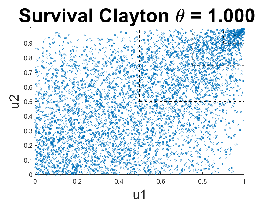
The Clayton copula above has large dependence at the corner. We instead define the so called ‘survival Clayton’ (SC) copula, in which the ‘survival’ relation holds for any copula, as:
| (6) |
and with copula density . Then, for distributed as the associated survival function (for the survival Clayton copula), , is defined as:
| (7) |
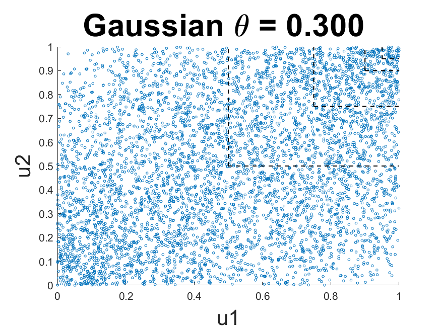
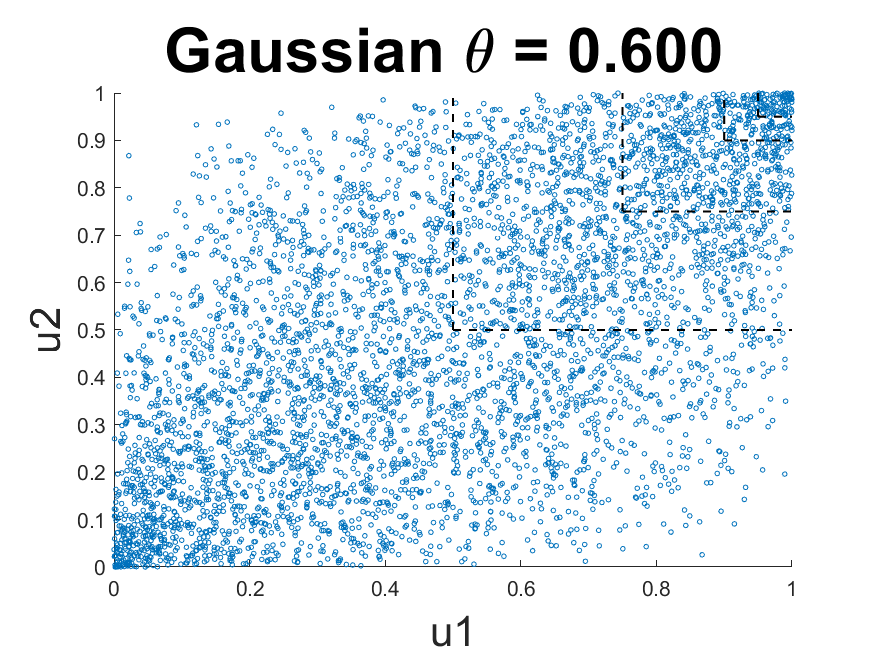
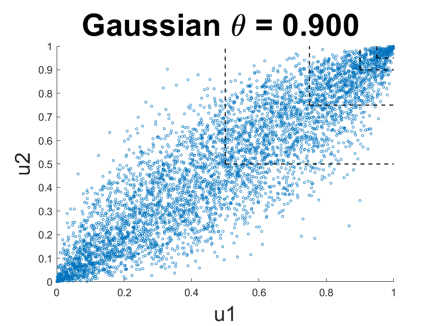
See figure 2 for sample draws from both the Gaussian copula and the survival Clayton copula.
3 Methodology
A motivating factor in analyzing anomaly scores with copulas is the removal of confounding marginal structure, especially in the tail where the precise marginal distribution is most difficult to estimate. We are interested in the similarity between variables, especially in the tails, not the marginal score distributions. And for anomaly scores in particular, we are only concerned with the score relationship in the upper quadrant only. Although where to define the upper quadrant requires further consideration below, working with copulas simplifies the situation through marginal standardization.
Let denote the (upper) q-quadrant As we are primarily interested in associations within we might attempt to fit the survival Clayton copula density only to sample points that lie in after marginal standardization, and estimate the association parameter . However, this has the undesirable property of simply favoring copula density models that have the greatest density inside of , regardless of the actual shape or fit within .
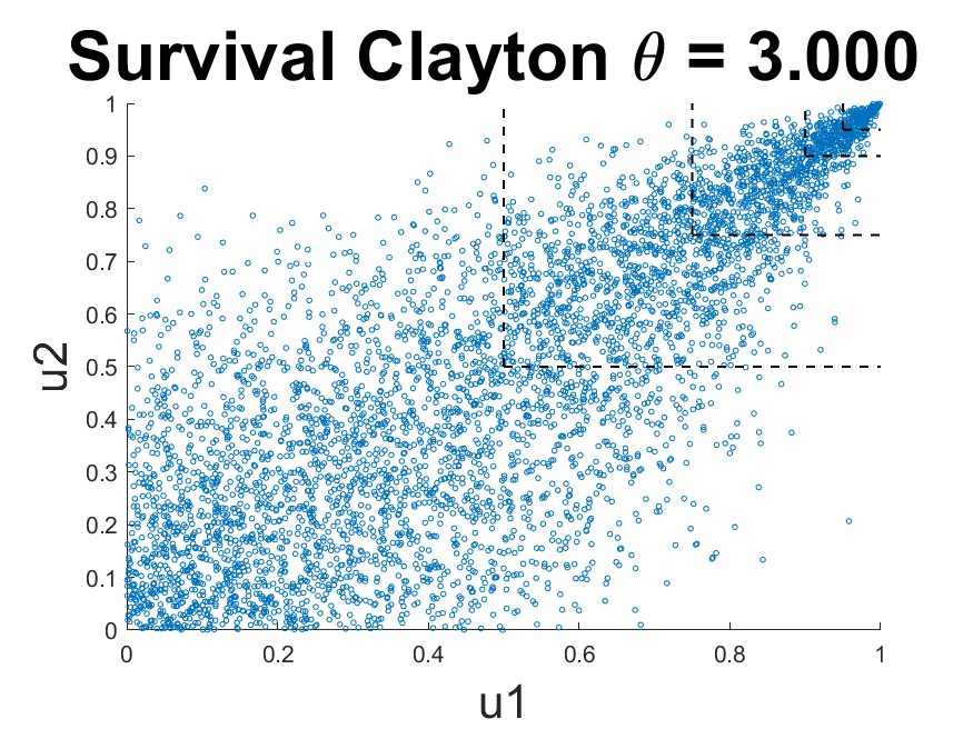
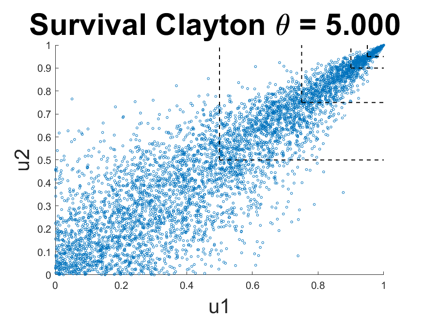
We thus propose deriving the conditional density specifically for the upper copula quadrant, and using properties of that density to define a similarity measure. Specifically, we define the q-quadrant conditional density of the survival Clayton copula as
| (8) |
We call the function the survival Clayton conditional (quantile or quadrant) density, and we note that it is not itself a copula, it is a conditional density derived from a copula. In particular the marginal distributions of are not uniform.
In practice, we do not expect samples directly from a copula. Instead, for a random sample , we apply variable-wise transformations (Ruppert and Matteson 2011) and define a semiparametric pseudo log-likelihood function as
| (9) |
in which
| (10) |
and is shorthand for .
3.1 Copula Quadrant Similarity
In order to create a similarity measure that is especially sensitive to upper tail dependence and agnostic to lower quadrant dependence, we utilize flexible copulae that can capture increasingly strong tail dependence. The survival Clayton copula exhibits varying degrees of increasing tail dependence as its single association parameter increases, and is shown to have superior tail dependence sensitivity to the Gaussian copula, see figures 3 and 4. In figure 3 we see the Clayton copula has faster changes of contours (both larger directional derivatives, as well as just generally higher density in this upper quadrant). For instance consider the directional derivative of the likelihoods in the [1,-1] direction: the Gaussian contours are nearly parallel to this, but the Clayton contours vary considerably, which shows they are sensitive to how dependent data are, that is, how close the data are to x=y line. Additionally, the Clayton copula possesses beneficial theoretical properties for modelling tail dependence: it is a natural limit for conditional bivariate extremes, which also have an Archimedean copula dependence structure; and is the only copula which is invariant under the upper q-quadrant conditioning we described above (Juri and Wüthrich 2002; Oakes 2005; Charpentier 2003).


To measure extremal similarity we propose using the association parameter that maximizes the log-likelihood given in equation 9, for a specific :
| (11) |
Although we have chosen the survival Clayton copula as our base measure, our definitions allow for the flexibility of choosing among other copula families, as long as an association parameter is indicative of tail dependence. The proposed will capture information about the shape of the tail dependence, how quickly it strengthens inside of . We find below that does well empirically for most values of , thus we propose using it as the first component of our similarity measure.
A weakness of is that it does not explicitly account for the fraction of points in , where . Whereas the empirical copula and empirical survival function , which are used to define , do (Coles et al. 1999). They are defined as
| (12) |
with , and . This last relation is only approximate due to both the finite and random nature of a sample. When using derived from the empirical distribution function (see equation 10), then there is at most an error of .
As an alternative copula quadrant similarity measure we propose matching the survival Clayton survival function with the empirical survival function to find the best association parameter . We define
| (13) |
There are many copulas that exhibit increasing tail dependence through increasing their sole association parameter (e.g., Joe, Clayton, Gumbel, Gaussian), with independence at a minimum and perfect dependence at a maximum (possibly infinite). For such copulae, the function is strictly monotonically increasing in . Thus as long as , that is there are more q-quadrant points than expected under independence, then equation 13 can be solved as an equality instead of minimization:
| (14) |
However, when , then the solution to equation 13, cannot be solved as an equality, but instead will have a boundary as the minimizer, which is where the copula family converges to the independent copula for the above mentioned copula families. In addition if then equation 13 cannot be solved as an equality, and in fact has no solution if the domain of is unbounded (informally is the solution). However it is guaranteed that if is computed using equation (10). One option if the is not computed using (10) is to bound the domain of , at least for the minimization in equation 13.
The similarity measures , , and are all based on a single measurement at of the empirical survival function or empirical copula. The proposed is model based, allowing it to inherit the tail dependent properties of the chosen model (i.e., the survival Clayton model), whereas and are model-free estimates of similarity using only and . Model based estimates such as and tend to have less variation than model free ones, and exhibit the tail dependence sensitivities of the base copula model from which they are derived from.
These two proposed estimators and complement each other well, capturing information about the strength of tail dependence inside of and the excess fraction inside of , respectively. The first, , is able to take into account tail shape (and dependence strength) information, but breaks down at larger , where there is not enough data to reliably estimate tail dependence. For these larger quantiles will be a more reliable estimator. In addition, assuming the survival Clayton model is well specified, the two estimators are consistent and asymptotically independent, which is proved in the Appendix (Khan 2004). Noting this asymptotic independence and the complementary strengths of both estimators, we define our Copula Quadrant Similarity Measure as the average of these two measures:
| (15) |
Larger values correspond to higher tail dependence or greater anomaly or extremal similarity, whereas value near imply tail independence.
The advantage of averaging the two estimators as opposed to either one individually is shown in figure 5. We see that the average is more stable over a broad range of , and often outperforms either one individually for values in desired range around . Empirical results shown below further demonstrate the effectiveness of as a measure of extremal or anomaly similarity, capturing the essential tail dependence through the survival Clayton copula.


4 Evaluation Details
A visual summary of the proposed methodological flow is shown in figure 6. The rest of this section goes over the details of each step.
4.1 Anomaly Score Similarity
We describe how this procedure is applied to measure the similarity between pairs of anomaly detection scoring algorithms. Anomalies are present in a given dataset where each is a datapoint in some not necessarily continuous space . We have access to anomaly detection algorithms , such that is the anomaly score given by algorithm on point (the higher the score, the more anomalous). We denote the matrix . Then the procedure discussed below can be applied, where the similarity between the pair of vector scores represents the similarity of algorithms and .
Using this dataset of scores, , we compute the pairwise column similarity. The first step is to transform the data onto the copula scale using the empirical cdf, equation 10. A value is chosen, we make the general recommendation of , but this can vary depending on application. For each pair of column indexes , the conditioned copula MLE estimator is fit on the pair [] using any convex optimization method (as the Clatyon copula density is convex in ). Similarly the estimator is fit on each pair by solving equation 14. The similarity measure is defined as in equation 15, as the average of the two estimators. We denote to be the matrix of pairwise similarity measures, is the similarity measure applied to columns and .
4.2 Alternative Similarity Measures
We want to compare our similarity measure, , with three main alternatives, , and “upper correlation” or “UCorr”. and were described in the introduction, see equations 1 and 2. We apply these to data by taking the empirical versions; the probabilities in equations 1 and 2 are replaced with the fraction of data in the relevant regions. “UCorr” is the correlation of the data in , which is called “uppertail conditional rank correlation” by Charpentier 2003. These alternatives will have the same flow as , in particular they are applied to the transformed variables and fit pairwise.

4.3 Spectral Clustering Visualization and Evaluation Metric
There is no clear choice to decide how good a certain similarity measure is since in general this is an unsupervised task. The approach we will take is to assume there is some ground truth clustering present. In the anomaly detection algorithm case this corresponds to the belief that a certain set of anomaly detection algorithms are similar to each other in that they give extreme scores to the same set of observations. In the data matrix case the belief is that certain variables (columns) are related to each other by having strong tail dependence. In order to evaluate our similarity measure using these assumed cluster assignments, we will first use our similarity measure to build a spectral embedding. A good description of spectral embedding is given by Von Luxburg 2007. Using the spectral embedding constructed from the pairwise similarity matrix , we can now quantitatively measure the performance of similarity measures when there is a clustering that is taken as ground truth. While there are many clustering objectives/loss functions to choose from, we employ the Davies-Bouldin index. The Davies-Bouldin index roughly measures the proportion of inter-cluster spread versus intra-cluster spread, see the Appendix.
5 Simulations and Experiments
5.1 Block Dataset
A scenario that is ideal to show the necessity of considering a similarity measure more complex than or is data generated from two blocks in the unit square. The lower left block will be on for , and data is uniformly distributed conditional on being inside the block. A more complex distribution is used for the upper block; we choose to create two clusters of four variables (columns) each. If a pair of variables come from the same cluster, then the upper block has the dependence of a Gaussian copula, see the left plot of figure 7. If the pair comes from variables of different clusters, than the two have an independent upper block, as in the right plot of figure 7. For , both and will be insensitive to that choice of upper right block, they will assign the same similarity measure if the upper block has tight dependence or is independent because they are simply a function of counting the number of points inside that block. By contrast our will strongly differentiate those two cases for any value of , since the shape and strength of tail dependence in the upper right quadrant strongly affects the copula fit. Spectral embeddings using the aforementioned similarity measures are shown in figure 7, and the DB-indexes of these embeddings shown in table 1. Both and fail to differentiate the red and blue clusters, they do not assign different similarities to the left and right plots in figure 7.


5.2 Mixture Dataset
A scenario that is motivated by anomaly detection is data generated from a mixture, with one mixture component considered anomalous, somewhat similar to copula mixtures defined by Tewari et al. 2011. The full description of this constructed dataset in is in the appendix, but in short the anomalous component is created by spiking only a subset of features. Pairs of these spiked features will possess stronger tail dependence due to these anomalies, whereas a pair of features containing one spiked dimension and one non-spiked dimension will lack tail dependence due to the lack of extreme anomaly features in the non-spiked dimension. The third type of pair, non-spiked vs non-spiked will have moderate tail dependence due to the general correlation of the non-anomalous component chosen for the dataset. These three types of pairs are shown in figure 9.


We show three different similarity measures, our , , and UCorr, all with the value in figure 10. A good similarity measure will assign significantly higher values of similarity of anomalous dimensions with other anomalous dimensions, which are those pairs show in red. We see that our proposed is the similarity measure that best separates these pairs, and is the only one that separates all three types of pairs. Our similarity measure is able to capture the tail dependence of the anomalous dimensions, although the anomalies are only a small fraction of the dataset. This was achieved due to the Clayton copula’s sensitivity to tail dependence. Results from the mixture dataset are also shown in table 1.


5.3 Two Anomaly Modes Dataset
We validate the proposed similarity measure to evaluate the similarity between anomaly detection algorithms on an ideal simulated dataset, which we name the TwoAnom dataset. This dataset is useful to analyze because it has two kinds of anomalies, whose anomalous behavior lie in two separate subspaces, see the appendix for the full description. In brief, for FAMD/PCA like algorithms, one kind of anomaly is revealed in the subspace containing the first few dimensions (first few principal coordinates), whereas the subspace containing the last few dimensions perform this separation for the second kind of anomaly. The anomaly scores for three example pairs are shown in figure 11. We expect a clustering of algorithms that use the first few dimensions, and a second cluster of algorithms that use the last few dimensions. We use these two clusters as ground truth and measure the Davies-Bouldin index across a variety of similarity measures, whose results are shown in table 1.


5.4 Experiments
We perform the full flow of the proposed methodology, as shown in figure 6, on several datasets. One is from the UCI machine learning repository (Dua and Graff 2017), and three from the ODDS anomaly detection repository Descriptions of these datasets are presented in the appendix. We apply PCA-like anomaly detection algorithms, where some of the algorithms make use of kurtosis, which has been shown to increase anomaly detection performance across several domains, see the appendix for more explanation of these algorithms (Davidow and Matteson 2020). We expect the kurtosis methods to be more accurate and similar to each other, as they extract similar features. Thus we expect a clustering of kurtosis methods, and measure the DB index based on this expected clustering, whose results are shown in table 1.
| Dataset | UCorr | |||
|---|---|---|---|---|
| Mnist | 0.072 | 0.075 | 0.313 | 0.321 |
| Ann | 0.063 | 0.114 | 0.111 | 0.114 |
| Two Anom | 0.001 | 0.037 | 0.004 | 0.005 |
| Mixture | 0.022 | 0.023 | 0.263 | 0.265 |
| Block | 0.016 | 0.047 | 4.804 | 4.838 |
| Musk | 0.762 | 1.059 | 1.015 | 1.023 |
| Shuttle | 0.611 | 1.086 | 0.841 | 0.842 |
6 Anomaly Score Combination
We illustrate how our similarity measure can be used to optimally combine anomalies scores from various methods in an unsupervised fashion Aggarwal and Sathe 2017; Aggarwal 2013. A principal component based unsupervised ensemble regression method is presented in Dror et al. 2017, however it is assumed predictors make independent errors, which is not a valid assumption in most realistic settings. A spectral clustering approach for an ensemble of unsupervised classifiers is shown in Jaffe et al. 2016. We present a similar method, except we have continuous anomaly scores, and these scores are on different scales. Thus we first put the anomaly scores on the same scale via equation 10. As we care most about the anomalies, i.e. the observations with the most extreme scores, we use our tail sensitive similarity measure to effectively cluster the scoring methods. This allows us to obtain a stronger signal within cluster, and to ignore methods which are not similar to any others, which are assumed to be noise.
We simulate a dataset by drawing from a t-distribution, chosen with a low number of degrees of freedom . This is chosen due to the heavy tailed property of this distribution, which will induce outliers which are many standard deviations from the mean. We note that a random variable is -distributed with degrees of freedom if where is a standard normal, and is independent of and chi-square distributed with degrees of freedom (Ruppert and Matteson 2011).
We partition variables into clusters and create dependence of variables within clusters by sharing the same within clusters. That is we let dimension of observation be: , where is the cluster index associated with . We create such clusters, each with three variables. I.e. We also create “noise” dimensions, which are chosen to be normally distributed instead of t-distributed. That is for , we define . We flag an observation as an outlier if its distance to the origin when projected to the subspace of the first 12 dimensions is among the top among all all observations. To simulate the scores of anomaly detection algorithms, we consider one algorithm per dimension of the dataset, whose score on observation is the absolute value of . That is we create 62 anomaly detectors, one for each dimension, where the anomaly detector uses the feature,
To effectively recover the ground truth clusters, a measure is required that is sensitive to tail dependence. We compute on all pairs of anomaly detection algorithms, forming the similarity matrix , where is the similarity defined by applied to the anomaly scores of ,. We transform this pairwise similarity matrix to a pairwise dissimilarity matrix with (exponential taken componentwise). We then employ the DBSCAN (Ester et al. 1996) clustering algorithm on this dissimilarity matrix. We find we can exactly recover the ground truth clusters.
We create an ensemble method by taking the mean rank within cluster, and the maximum rank across these means. This allows us to produce a stronger signal within cluster, while picking up different anomalies picked out by different clusters by choosing the max function (Aggarwal 2015). This is compared to taking the mean rank across all algorithms, and the max rank across all algorithms. We objectively measure the performance of these ensemble methods by computing the Area Under the Curve of the Receving Operating Characteristic (AUC ROC), which is the area under the curve of true positives rate versus false positive rate. The AUC ROC can be interpreted as the probability a random outlier is assigned a higher score than a random inlier.
| Combine Across/Within | All | Mean | Max |
| Mean | 0.692 | 0.864 | 0.684 |
| Max | 0.864 | 0.999 | 0.875 |
7 Discussion
Our model outperforms ,, and UCorr because the survival Clayton copula puts heavy mass in the upper right tail. The similarity measure using the upper quadrant of the survival Clayton copula has been demonstrated to be sensitive to tail dependence, which is often induced only by a small fraction of extreme anomalous observations. By constructing such a similarity measure that is sensitive to this small but important fraction, one can better solve downstream tasks, such as clustering the algorithms together, recognizing risk, and ultimately combining anomaly scoring algorithms together optimally.
Comparison with and . at a fixed level of is simply a function the fraction of points inside of . All points inside are counted equally for , despite the important additional information such as if they are in the top right versus the other corners. This is similar to our . However our full approach using the average of both and incorporates the shape and tail dependence strength information by making use of Clayton copula’s density function, assigning higher likelihood to points in the top right corner. It is for this reason that our method is able to better suited to measure similarity across a wide range of , even at values far lower than the anomaly percentage, which may be unknown.
Comparison with UCorr. The density of the Clayton copula is ideal to measure similarity that is sensitive to extreme value anomalies. Using UCorr is somewhat similar to our measure, however better captures upper tail dependence. In particular, UCorr is symmetric and does not focus on the upper tails. Further, correlation is not as sensitive to strong tail dependence and instead measures central tendencies, as compared with our highly sensitive proposed measure .
The similarity measure using the upper right quadrant of copulas is both novel and excellently sensitive to extreme value dependence. The survival Clayton copula is well suited for this context because of its large extreme value dependence, performing significantly better than the Gaussian copula. Upper correlation has inadequate sensitivity to tail dependency. and at fixed capture information only about the number of points in , which is also captured by our proposed . However our method includes the more complex , which when averaged with creates a robust measure of tail dependence.
Appendix
8 Davies Bouldin Index
We termed the spectral embedding space , thus is the coordinate of observation after spectral embedding. As all of the examples considered consisted of only two clusters, we used a one dimensional spectral embedding. However this can be modified to higher dimensional embeddings for different problems with more than two clusters. This one dimensional embedding is , it is the second column of , the first column of contains no useful information as it corresponds to the zero eigenvalue, and is proportional to the vector of all ones. Now we present the necessary definitions for the Davies-Bouldin Index.
For each cluster the inter-cluster spread is defined as , where is the centroid of cluster ,and is the set associated with cluster . The intra cluster distance is defined between cluster centers , . From this a pairwise loss function is defined between clusters , and the loss of a single cluster is defined as . The Davies-Bouldin index as defined as Where in our examples = 2 is the number of clusters. For clusters than are well separated, is small compared to , and thus the Davies-Bouldin index is small.
9 Data Description
9.1 Mixture Model
Tewari (2011) defines a copula generated from a Gaussian Mixture Model. We use a slightly different model; there are two mixture components, inliers generated from a dimensional multivariate normal with pairwise correlation , and anomalies generated with pairwise correlation , whose first dimensions are scaled by a factor . The reason for spiking only the first dimensions is to create a clustering of columns, the first columns have similar extreme points (the anomalies), whereas the rest of the columns have more independent extreme points. Absolute values are taken of the dataset so the anomalous behavior lies only in the upper tail. The data set is generated by drawing 5000 inliers and 200 anomalies from the above mentioned multivariate Gaussians, taking the absolute value of all features, then taking the empirical CDF transform, equation 10 in the main paper so the data is on the copula scale. There are three kinds of pairs generated from such a model, an anomalous column with another anomalous column, an anomalous column with a regular, and a regular with a regular.
9.2 Two Anom Dataset Description
We aim to create a dataset with two different kinds of anomalies picked up in two different subspaces. We create a dataset with latent dimension 100, where the main variation of the inliers is only among a 30 dimensional “true” subspace, variation on the remaining 70 dimensional subspace is a factor of 100 smaller. One set of anomalies has the same covariance structure on this 30 dimensional subspace, but more noise (larger magnitude by a factor of 30) on the remaining 70 dimensional subspace as compared to the inliers. The second set of inliers is “spiked” (larger magnitude by a factor of 3) on a 5 dimensional subspace of the 30 dimensional “true” subspace, with identical structure to the inliers on the remaining 95 dimensional subspace. We create such a dataset with 5000 inliers, and 200 total anomalies, 100 of each of these two types. The first type of anomaly is separated by the smallest principal components, as those are the noise components of inliers which these anomalies differ on. The second type of anomaly is separated by the largest principal components, since these anomalies contribute to these components making them the largest. We use a set of four anomaly detection algorithms that make use the first principal components, and a set of four anomaly detection algorithms that make use of the last principal components, as described in (Davidow, 2020).
9.3 Experimental Datasets
We use an anomaly detection dataset from the UCI machine learning repository, called the ann dataset. We use three different anomaly detection from the ODDS dataset, Mnist, Musk and Shuttle. More detailed descriptions of those are found at the ODDS site (Ray). We show summary statistics of these datsets in table 3.
| Dataset | Observations | Dimensions | Outliers(%) |
|---|---|---|---|
| Mnist | 7603 | 100 | 700 (9.2%) |
| Ann | 7200 | 21 | 533(7.4%) |
| Musk | 3062 | 166 | 97 (3.2%) |
| Shuttle | 49097 | 9 | 3511 (7.0%) |
We apply PCA-like anomaly detection algorithms, where some of the algorithms make use of kurtosis, which has been shown to be more accurate and similar to each other, as they extract similar features which has been shown to increase anomaly detection performance across several domains (Davidow, 2020).
9.4 Correlation between and
The claim was made in the original paper that the correlation between and is small when the survival Clayton model is well specified. We motivate this numerically by drawing survival clayton samples with three different values of with . For each sample and are computed. The sample correlation of and are computed for each using complete redraws of the samples. The resulting sample correlations of these redraws were for , respectively. These two estimators have small bias, and also do not have a large positive correlation, and thus a weighted combination of them will produce a superior estimator.
We prove that and are both unbiased up to order .
The setting is that independent samples are drawn with the survival Clayton distribution, equation 7 in the main paper, with true parameter . We begin by proving that has bias . As a reminder we defined with . Since each is iid, is binomially distributed, with trials and success parameter . Recall , and recall that can be solved by equation 14 in the main paper, thus if we denote then we see conditional on is a deterministic function of :
.
We know has an inverse because is strictly monotonic in . However there are boundary issues when and when , for these we define as and respectively for some arbitrary but finite . In order for and to have bias the true must satisfy .
Thus . At any fixed is w.r.t , so is also by the inverse function theorem, at least for (i.e. at least in some interval around ). Thus we can appeal to the results of Khan (2004), to conclude
where is the variance of the indicator variable . is independent of , and is the true since . Thus, the bias is .
Now we turn our attention to , and prove that it is unbiased up to . We again put a bound on the estimator, the space over which is optimizied is on , and this estimator is unbiased up to only when the true . We also let take the value when = 0, although this will happen with exponentially small probability in .
Of critical importance is that the definition of coincides with that of the maximum likelihood estimator for the distribution in equation 8 from the main paper. Thus when there are points inside of , is unbiased up to order That is
Where is the bias of the MLE when there are data, in particular is since is a maximum likelihood estimator, and is bounded since we have defined a bounded .
We first argue the first summation is less than . We use the central limit theorem approximation to the binomially distributed , which has mean and variance . The upper bound of the sum is standard deviations from the mean, and thus appealing to the normals cdf asymptotics, is , which in particular is .
The second summation is since is . To spell it out, we have for some , . For notational simplicity we let . As is a decreasing function, . Using this we can bound
This last bound is (since ), thus the bias of is also .
9.5 Asymptotic Independence
In fact we can prove along similar lines that and are asymptotically independent. To make this precise, we define the shifted and scaled estimators as indexed by : and .
The results of Khan (2004) also prove that the variance of decreases with , thus converges in distribution to for correctly chosen .
We let . We rely heavily on the fact that the definition of coincides with the definition of the maximum likelihood estimator of data drawn independently inside of according to equation (8) in the main paper. Thus corresponds to the cdf of a shifted and scaled maximum likelihood estimator, and thus with the correct choice of , , where is the standard normal’s cdf.
Theorem: and are asymptotically independent
Proof The definition of asymptotic independence is that the multivariate distribution of the pair of random sequences converges to the joint distribution of independent random variables. Thus we aim to prove the following convergence statement:
as , where is the two dimensional multivariate centered normal cumulative distribution function whose covariance matrix is the 2 by 2 identity matrix.
We need to show that and , that such that By the fact that and both converge in distribution to a standard normal, we know and such that , , and . We choose at least large enough so that , e.g. . We denote for notational simplicity. We proceed along the same lines as above to compute the probability of interest, , by conditioning on possible values of . Given the condition , the largest relevant value of is , obtained by solving from the equation defining , i.e. . Thus,
| (16) | ||||
| (17) | ||||
| (18) | ||||
| (19) |
In (16) we used the fact that conditional on the event = , is a deterministic monotonic function of (thus it is conditionally independent of conditioned on ), and (17) follows since when . In (18) we re-wrote the conditional cdf of using the definition of . In (19) we break this sum into the same two parts as done previously, from to , and to . The first part from to is along the same reasoning as shown in section 2.4. To be explicit, and so , and was shown to be in section 2.4, and thus can be made arbitrarily small with a large enough choice of . However we have made use of an implicit assumption that . This can always be made true with a large enough choice of (which importantly may depend on ), since choosing arbitrarily large one can make arbitrarily close to .
We focus on the second part,
Note that depends on since the upper bound depends on . Recall that for all , converges to , that is , the difference . We denote . Thus, we can bound the difference of and using the triangle inequality, . This can be further manipulated with the triangle inequality to bring us closer to our desired inequality relating and :
| (20) |
We now aim to bound , we use the fact that is a monotonic function of , thus We have shown is , thus is , or informally . Since , we know that , and thus (also informally):
Plugging this bound for into (20), we can bound the difference (by the triangle inequality):
As is bounded between and , and is allowed to depend on and , this error can be driven arbitrarily small for small enough choices of , and a large enough choice of . We recall that is the second portion of the sum of the probability of interest , but the first part was shown to be , and thus the error can be driven arbitrarily small, and so the estimators are asymptotically independent.
The intuition behind the asymptotic independence of and is that is estimating the “shape” inside, and the number of points inside does not influence the shape but only how densely the shape is filled in. This intuition suggests that the two estimators may be independent (not just asymptotically), but we conjecture this is not the case, mainly due to the numerically sampled correlations cited above, which we found to interestingly be consistently negative. This dependence between the two is possibly due to a dependence of the bias of on , it is only asymptotically unbiased, which is why the pair of estimators is only asymptotically independent.
10 Main Results
Due to brevity we only presented results at in the main paper. However here we show results for
| Dataset | UCorr | —— | UCorr | ||||||
|---|---|---|---|---|---|---|---|---|---|
| Mnist | 0.248 | 0.264 | 0.494 | 0.507 | —— | 0.072 | 0.075 | 0.313 | 0.321 |
| Ann | 0.251 | 0.139 | 0.475 | 0.521 | —— | 0.063 | 0.114 | 0.111 | 0.114 |
| Two Anom | 0.001 | 0.021 | 0.005 | 0.009 | —— | 0.001 | 0.037 | 0.004 | 0.005 |
| Mixture | 0.029 | 0.058 | 0.149 | 0.154 | —— | 0.022 | 0.023 | 0.263 | 0.265 |
| Block | 0.033 | 0.132 | 2.177 | 2.153 | —— | 0.016 | 0.047 | 4.804 | 4.838 |
| Musk | 0.804 | 0.870 | 0.966 | 1.123 | —— | 0.762 | 1.059 | 1.015 | 1.023 |
| Shuttle | 0.418 | 0.828 | 0.434 | 0.503 | —— | 0.611 | 1.086 | 0.841 | 0.842 |
| Dataset | UCorr | —— | UCorr | ||||||
|---|---|---|---|---|---|---|---|---|---|
| Mnist | 0.024 | 0.065 | 0.060 | 0.053 | —— | 0.030 | 0.072 | 0.151 | 0.117 |
| Ann | 0.069 | 0.104 | 0.112 | 0.100 | —— | 0.061 | 0.244 | 0.071 | 0.062 |
| Two Anom | 0.000 | 0.120 | 0.014 | 0.008 | —— | 0.075 | 0.575 | 0.024 | 0.007 |
| Mixture | 0.006 | 0.040 | 0.059 | 0.054 | —— | 0.003 | 0.434 | 0.039 | 0.028 |
| Block | 0.011 | 0.058 | 0.040 | 0.039 | —— | 0.009 | 0.174 | 0.041 | 0.034 |
| Musk | 0.777 | 1.148 | 0.956 | 0.952 | —— | 0.800 | 1.037 | 0.836 | 0.843 |
| Shuttle | 0.964 | 1.199 | 1.060 | 1.059 | —— | 0.913 | 6.234 | 1.199 | 1.212 |
References
- Aggarwal (2013) C. C. Aggarwal. Outlier ensembles: position paper. ACM SIGKDD Explorations Newsletter, 14(2):49–58, 2013.
- Aggarwal (2015) C. C. Aggarwal. Outlier analysis. In Data mining, pages 237–263. Springer, 2015.
- Aggarwal and Sathe (2017) C. C. Aggarwal and S. Sathe. Outlier ensembles: An introduction. Springer, 2017.
- Ahsen et al. (2019) M. E. Ahsen, R. M. Vogel, and G. A. Stolovitzky. Unsupervised evaluation and weighted aggregation of ranked classification predictions. Journal of Machine Learning Research, 20(166):1–40, 2019.
- Beirlant et al. (2006) J. Beirlant, Y. Goegebeur, J. Segers, and J. L. Teugels. Statistics of extremes: theory and applications. John Wiley & Sons, 2006.
- Bernard and Czado (2015) C. Bernard and C. Czado. Conditional quantiles and tail dependence. Journal of Multivariate Analysis, 138:104–126, 2015.
- Bücher et al. (2015) A. Bücher, S. Jäschke, and D. Wied. Nonparametric tests for constant tail dependence with an application to energy and finance. Journal of Econometrics, 187(1):154–168, 2015.
- Caillault and Guegan (2005) C. Caillault and D. Guegan. Empirical estimation of tail dependence using copulas: application to asian markets. Quantitative Finance, 5(5):489–501, 2005.
- Capéraà et al. (1997) P. Capéraà, A.-L. Fougères, and C. Genest. A nonparametric estimation procedure for bivariate extreme value copulas. Biometrika, 84(3):567–577, 1997.
- Cebrián et al. (2003) A. C. Cebrián, M. Denuit, P. Lambert, et al. Analysis of bivariate tail dependence using extreme value copulas: An application to the soa medical large claims database. Belgian Actuarial Journal, 3(1):33–41, 2003.
- Chang et al. (2016) Y. Chang, Y. Li, A. Ding, and J. Dy. A robust-equitable copula dependence measure for feature selection. In Artificial Intelligence and Statistics, pages 84–92, 2016.
- Charpentier (2003) A. Charpentier. Tail distribution and dependence measures. In Proceedings of the 34th ASTIN Conference, pages 1–25, 2003.
- Chesnay and Jondeau (2001) F. Chesnay and E. Jondeau. Does correlation between stock returns really increase during turbulent periods? Economic Notes, 30(1):53–80, 2001.
- Coles et al. (1999) S. Coles, J. Heffernan, and J. Tawn. Dependence measures for extreme value analyses. Extremes, 2(4):339–365, 1999.
- Coles and Powell (1996) S. G. Coles and E. A. Powell. Bayesian methods in extreme value modelling: a review and new developments. International Statistical Review/Revue Internationale de Statistique, pages 119–136, 1996.
- Currie (1999) J. Currie. “directory of coefficients of tail dependence,”department of mathematics and statistics technical report. Technical report, ST-99-06, Lancaster University, 1999.
- Davidow and Matteson (2020) M. Davidow and D. S. Matteson. Factor analysis of mixed data for anomaly detection. arXiv preprint arXiv:2005.12129, 2020.
- Davison and Smith (1990) A. C. Davison and R. L. Smith. Models for exceedances over high thresholds. Journal of the Royal Statistical Society: Series B (Methodological), 52(3):393–425, 1990.
- Dror et al. (2017) O. Dror, B. Nadler, E. Bilal, and Y. Kluger. Unsupervised ensemble regression. arXiv preprint arXiv:1703.02965, 2017.
- Dua and Graff (2017) D. Dua and C. Graff. UCI machine learning repository, 2017. URL http://archive.ics.uci.edu/ml.
- Ester et al. (1996) M. Ester, H.-P. Kriegel, J. Sander, X. Xu, et al. A density-based algorithm for discovering clusters in large spatial databases with noise. In Kdd, volume 96, pages 226–231, 1996.
- Hyvärinen and Oja (2000) A. Hyvärinen and E. Oja. Independent component analysis: algorithms and applications. Neural networks, 13(4-5):411–430, 2000.
- Jaffe et al. (2016) A. Jaffe, E. Fetaya, B. Nadler, T. Jiang, and Y. Kluger. Unsupervised ensemble learning with dependent classifiers. In Artificial Intelligence and Statistics, pages 351–360, 2016.
- Joe (1997) H. Joe. Multivariate models and multivariate dependence concepts. CRC Press, 1997.
- Jondeau and Rockinger (2006) E. Jondeau and M. Rockinger. The copula-garch model of conditional dependencies: An international stock market application. Journal of international money and finance, 25(5):827–853, 2006.
- Juri and Wüthrich (2002) A. Juri and M. V. Wüthrich. Copula convergence theorems for tail events. Insurance: Mathematics and Economics, 30(3):405–420, 2002.
- Khan (2004) R. A. Khan. Approximation for the expectation of a function of the sample mean. Statistics, 38(2):117–122, 2004.
- Ledford and Tawn (1996) A. W. Ledford and J. A. Tawn. Statistics for near independence in multivariate extreme values. Biometrika, 83(1):169–187, 1996.
- Mendes et al. (2007) B. V. Mendes, E. F. de Melo, and R. B. Nelsen. Robust fits for copula models. Communications in Statistics—Simulation and Computation®, 36(5):997–1017, 2007.
- Oakes (2005) D. Oakes. On the preservation of copula structure under truncation. The Canadian Journal of Statistics/La revue canadienne de statistique, pages 465–468, 2005.
- Parisi et al. (2014) F. Parisi, F. Strino, B. Nadler, and Y. Kluger. Ranking and combining multiple predictors without labeled data. Proceedings of the National Academy of Sciences, 111(4):1253–1258, 2014.
- Peng et al. (2005) H. Peng, F. Long, and C. Ding. Feature selection based on mutual information criteria of max-dependency, max-relevance, and min-redundancy. IEEE Transactions on pattern analysis and machine intelligence, 27(8):1226–1238, 2005.
- Poon et al. (2004) S.-H. Poon, M. Rockinger, and J. Tawn. Extreme value dependence in financial markets: Diagnostics, models, and financial implications. The Review of Financial Studies, 17(2):581–610, 2004.
- Poulin et al. (2007) A. Poulin, D. Huard, A.-C. Favre, and S. Pugin. Importance of tail dependence in bivariate frequency analysis. Journal of Hydrologic Engineering, 12(4):394–403, 2007.
- Ruppert and Matteson (2011) D. Ruppert and D. Matteson. Statistics and data analysis for financial engineering, volume 13. Springer, 2011.
- Rüschendorf (2009) L. Rüschendorf. On the distributional transform, sklar’s theorem, and the empirical copula process. Journal of Statistical Planning and Inference, 139(11):3921–3927, 2009.
- Serinaldi (2008) F. Serinaldi. Analysis of inter-gauge dependence by kendall’s k, upper tail dependence coefficient, and 2-copulas with application to rainfall fields. Stochastic Environmental Research and Risk Assessment, 22(6):671–688, 2008.
- Tewari et al. (2011) A. Tewari, M. J. Giering, and A. Raghunathan. Parametric characterization of multimodal distributions with non-gaussian modes. In 2011 IEEE 11th International Conference on Data Mining Workshops, pages 286–292. IEEE, 2011.
- Von Luxburg (2007) U. Von Luxburg. A tutorial on spectral clustering. Statistics and computing, 17(4):395–416, 2007.
- Wolpert and Wolf (1995) D. H. Wolpert and D. R. Wolf. Estimating functions of probability distributions from a finite set of samples. Physical Review E, 52(6):6841, 1995.
*