跳到论文正文
W Papers独立论文阅读器 arXiv:2101.02307 论文正文 计算阅读时间 · 0%
引用这篇论文根据当前论文元数据生成,正式投稿前建议核对。


License: arXiv.org perpetual non-exclusive license
arXiv:2101.02307v3 [stat.ML] 13 Sep 2022

Directed mixed membership stochastic blockmodel

Huan Qing qinghuan@cumt.edu.cn Affiliation: School of Mathematics Affiliation: China University of Mining and Technology Affiliation: Xuzhou, 221116, P.R. China    Jingli Wang jlwang@nankai.edu.cn Affiliation: School of Statistics and Data Science Affiliation: Nankai University Affiliation: Tianjin, 300071, P.R. China
Abstract

Mixed membership problem for undirected network has been well studied in network analysis recent years. However, the more general case of mixed membership for directed network in which nodes can belong to multiple communities remains a challenge. Here, we propose an interpretable and identifiable model: directed mixed membership stochastic blockmodel (DiMMSB) for directed mixed membership networks. DiMMSB allows that row nodes and column nodes of the adjacency matrix can be different and these nodes may have distinct community structure in a directed network. We also develop an efficient spectral algorithm called DiSP designed based on simplex structures inherent in the left and right singular vectors of the population adjacency matrix to estimate the mixed memberships for both row nodes and column nodes in a directed network. We show that DiSP is asymptotically consistent under mild conditions by providing error bounds for the inferred membership vectors of each row node and each column node using delicate spectral analysis. Numerical results on computer-generated directed mixed membership networks support our theoretical findings and show that our DiSP outperforms its competitor in both error rates and run-time. Applications of DiSP to real-world directed networks demonstrate the advantages of DiSP in studying the asymmetric structure of directed networks.

††shortheadings: DiMMSB / Qing and Wang††firstpage: 1
keywords
Community detection, Ideal Simplex, overlapping directed network, sparsity, spectral clustering, SVD.

1 Introduction

Networks with meaningful structures are ubiquitous in our daily life in the big data era. For example, the social networks generated by social platforms (such as, Facebook, Twitter, Wechat, Instagram, WhatsUp, Line, etc) provide relationships or friendships among users; the protein-protein interaction networks record the relationships among proteins; the citation networks reflect authors’ research preferences Dunne et al. 2002; Newman 2004; Notebaart et al. 2006; Pizzuti 2008; Gao et al. 2010; Lin et al. 2012; Su et al. 2010; Scott and Carrington 2014; Bedi and Sharma 2016; Wang et al. 2020. To analyze networks mathematically, researchers present them in a form of graph in which subjects/individuals are presented by nodes, and the relationships are measured by the edges, directions of edges and weights. Community detection is one of the major tools to extract structural information from these networks.

For simplification, most researchers study the undirected networks for community detection such as Lancichinetti and Fortunato 2009; Goldenberg et al. 2010; Karrer and Newman 2011; Qin and Rohe 2013; Lei and Rinaldo 2015; Jin 2015; Chen et al. 2018. The Stochastic Blockmodel (SBM) Holland et al. 1983 is a classical and widely used model to generate undirected networks. SBM assumes that one node only belongs to one community and the probability of a link between two nodes depends only on the communities memberships of the two nodes. SBM also assumes the nodes within each community have the same expected degrees. Abbe 2017 proposed a review on recent developments about SBM. While, in real cases some nodes may share among multiple communities with different degrees, which is known as mixed membership (also known as overlapping) networks. Airoldi et al. 2008 extended SBM to mixed membership networks and designed the Mixed Membership Stochastic Blockmodel (MMSB). Substantial algorithms have been developed based on MMSB, such as Gopalan and Blei 2013; Jin et al. 2017; Mao et al. 2017; Mao et al. 2020; Zhang et al. 2020.

Directed networks such as citation networks, protein-protein interaction networks and the hyperlink network of websites are also common in our life. Such directed networks are more complex since they often involve two types of information, sending nodes and receiving nodes. For instance, in a citation network, one paper may cite many other papers, then this paper can be labeled as ‘sending node’ and these cited papers can be labeled as ‘receiving nodes’. Several interesting works have been developed for directed networks. Rohe et al. 2016 proposed a model called Stochastic co-Blockmodel (ScBM) to model networks with directed (asymmetric) relationships where nodes have no mixed memberships (i.e., one node only belongs to one community). Wang et al. 2020 studied the theoretical guarantee for the algorithm D-SCORE Ji and Jin 2016 which is designed based on the degree-corrected version of ScBM. Lim et al. 2018 proposed a flexible noise tolerant graph clustering formulation based on non-negative matrix factorization (NMF), which solves graph clustering such as community detection for either undirected or directed graphs. In the bipartite setting some authors constructed new models by extending SBM, such as Zhou and Amini 2018; Razaee et al. 2019. The above models and algorithms for directed network community detection focus on non-mixed membership directed networks. Similar as in undirected networks, in reality, there exist a lot of directed networks such that their sending nodes and/or receiving nodes may belong to multiple clusters.

For the directed network with mixed memberships, Airoldi et al. 2013 proposed a multi-way stochastic blockmodel with Dirichlet distribution which is an extension of the MMSB model Airoldi et al. 2008, and applied the nonparametric methods, collapsed Gibbs sampling and variational Expectation-Maximization to make inference. In this paper, we focus on the directed network with mixed memberships and aim at developing a provably consistent spectral algorithm to estimate network memberships.

Our contributions in this paper are as follows:

  • (i)

    We propose a generative model for directed networks with mixed memberships, the Directed Mixed Membership Stochastic Blockmodel (DiMMSB for short). DiMMSB allows that nodes in a directed network can belong to multiple communities. The proposed model also allows that sending nodes (row nodes) and receiving nodes (column nodes) can be different, that is, the adjacency matrix could be an non-square matrix. The identifiability of DiMMSB is verified under common constraints for mixed membership models.

  • (ii)

    We construct a fast spectral algorithm, DiSP, to fit DiMMSB. DiSP is designed based on the investigation that there exist a Row Ideal Simplex structure and a Column Ideal Simplex structure in the right singular vectors and the left singular vectors of the population adjacency matrix. To scale the sparsity of a directed mixed membership network, we introduce the sparsity parameter. By taking the advantage of the recent row-wise singular vector deviation Chen et al. 2020 and the equivalence algorithm of DiSP, we obtain the upper bounds of error rates for each row node and each column node, and show that our method produces asymptotically consistent parameter estimations under mild conditions on the network sparsity by delicate spectral analysis. To our knowledge, this is the first work to establish consistent estimation for an estimation algorithm for directed mixed membership (overlapping) network models. Meanwhile, numerical results on substantial simulated directed mixed membership networks show that DiSP is useful and fast in estimating mixed memberships, and results on real-world data demonstrate the advantages on DiSP in studying the asymmetric structure and finding highly mixed nodes in a directed network.

Notations. We take the following general notations in this paper. For a vector xx, ‖x‖q\|x\|_{q} denotes its lql_{q}-norm. M′M^{\prime} is the transpose of the matrix MM, and ‖M‖\|M\| denotes the spectral norm, and ‖M‖F\|M\|_{F} denotes the Frobenius norm. ‖X‖2→∞\|X\|_{2\rightarrow\infty} denotes the maximum l2l_{2}-norm of all the rows of the matrix XX. Let σi​(M)\sigma_{i}(M) and λi​(M)\lambda_{i}(M) be the ii-th largest singular value and its corresponding eigenvalue of matrix MM ordered by the magnitude. M(i,:)M(i,:) and M(:,j)M(:,j) denote the ii-th row and the jj-th column of matrix MM, respectively. M(Sr,:)M(S_{r},:) and M(:,Sc)M(:,S_{c}) denote the rows and columns in the index sets SrS_{r} and ScS_{c} of matrix MM, respectively. For any matrix MM, we simply use Y=max⁡(0,M)Y=\mathrm{max}(0,M) to represent Yi​j=max⁡(0,Mi​j)Y_{ij}=\mathrm{max}(0,M_{ij}) for any i,ji,j.

2 The directed mixed membership stochastic blockmodel

In this section we introduce the directed mixed membership stochastic blockmodel. First we define a bi-adjacency matrix A∈{0,1}nr×ncA\in\{0,1\}^{n_{r}\times n_{c}} such that for each entry, A⁡(i,j)=1A(i,j)=1 if there is a directional edge from row node ii to column node jj, and A⁡(i,j)=0A(i,j)=0 otherwise, where nrn_{r} and ncn_{c} indicate the number of rows and the number of columns, respectively (the followings are similar). So, the ii-th row of AA records how row node ii sends edges, and the jj-th column of AA records how column node jj receives edges. Let Sr={i:iisarownode,1≤i≤nr}S_{r}=\{i:i\mathrm{~is~a~row~node},1\leq i\leq n_{r}\}, and Sc={j:jisacolumnnode,1≤j≤nc}S_{c}=\{j:j\mathrm{~is~a~column~node},1\leq j\leq n_{c}\}. In this paper, we assume that the row (sending) nodes can be different from the column (receiving) nodes, and the number of row nodes and the number of columns are not necessarily equal. We assume the row nodes of AA belong to KK perceivable communities (call row communities and we also call them sending clusters occasionally in this paper)

𝒞r(1),𝒞r(2),…,𝒞r(K),\displaystyle\mathcal{C}^{(1)}_{r},\mathcal{C}^{(2)}_{r},\ldots,\mathcal{C}^{(K)}_{r}, (1)

and the column nodes of AA belong to KK perceivable communities (call column communities and we also call them receiving clusters occasionally in this paper)

𝒞c(1),𝒞c(2),…,𝒞c(K).\displaystyle\mathcal{C}^{(1)}_{c},\mathcal{C}^{(2)}_{c},\ldots,\mathcal{C}^{(K)}_{c}. (2)

Let Πr∈ℝnr×K\Pi_{r}\in\mathbb{R}^{n_{r}\times K} and Πc∈ℝnc×K\Pi_{c}\in\mathbb{R}^{n_{c}\times K} be row nodes membership matrix and column nodes membership matrix respectively, such that Πr(i,:)\Pi_{r}(i,:) is a 1×K1\times K Probability Mass Function (PMF) for row node ii, Πc(j,:)\Pi_{c}(j,:) is a 1×K1\times K PMF for column node jj, and

Πr​(i,k)​is​the​weight​of​row​node​i​on​𝒞r(k),1≤k≤K,\displaystyle\Pi_{r}(i,k)\mathrm{~is~the~weight~of~row~node~}i~\mathrm{on~}\mathcal{C}^{(k)}_{r},1\leq k\leq K, (3)
Πc​(j,k)​is​the​weight​of​column​node​j​on​𝒞c(k),1≤k≤K.\displaystyle\Pi_{c}(j,k)\mathrm{~is~the~weight~of~column~node~}j~\mathrm{on~}\mathcal{C}^{(k)}_{c},1\leq k\leq K. (4)

We call row node ii ‘pure’ if Πr(i,:)\Pi_{r}(i,:) degenerates (i.e., one entry is 1, all others K−1K-1 entries are 0) and ‘mixed’ otherwise. Same definitions hold for column nodes.

Define a probability matrix P∈ℝK×KP\in\mathbb{R}^{K\times K} which is an nonnegative matrix and for any 1≤k,l≤K,1\leq k,l\leq K,

P⁡(k,l)∈[0,1].\displaystyle P(k,l)\in[0,1]. (5)

Note that since we consider directed mixed membership network in this paper, PP may be asymmetric. For all pairs of (i,j)(i,j) with 1≤i≤nr,1≤j≤nc1\leq i\leq n_{r},1\leq j\leq n_{c}, DiMMSB assumes that A⁡(i,j)A(i,j) are independent Bernoulli random variables satisfying

ℙ⁡(A⁡(i,j)=1)=∑k=1K∑l=1KΠr​(i,k)​Πc​(j,l)​P​(k,l).\displaystyle\mathbb{P}(A(i,j)=1)=\sum_{k=1}^{K}\sum_{l=1}^{K}\Pi_{r}(i,k)\Pi_{c}(j,l)P(k,l). (6)
Definition 1.

Call model (1)-(6) as the Directed Mixed Membership Stochastic Blockmodel (DiMMSB) and denote it by D​i​M​M​S​B​(nr,nc,K,P,Πr,Πc)DiMMSB(n_{r},n_{c},K,P,\Pi_{r},\Pi_{c}).

DiMMSB can be deemed as an extension of some previous models.

  • •

    When all row nodes and column nodes are pure, our DiMMSB reduces to ScBM with KK row clusters and KK column clusters Rohe et al. 2016.

  • •

    When Πr(i,:)\Pi_{r}(i,:) and Πc(j,:)\Pi_{c}(j,:) follow Dirichlet distribution for 1≤i≤nr1\leq i\leq n_{r} and 1≤j≤nc1\leq j\leq n_{c}, DiMMSB reduces to the two-way stochastic blockmodels with Bernoulli distribution Airoldi et al. 2013.

  • •

    When Πr=Πc\Pi_{r}=\Pi_{c} and P=P′P=P^{\prime}, Πr(i,:)\Pi_{r}(i,:) follow Dirichlet distribution for 1≤i≤nr1\leq i\leq n_{r}, and all row nodes and column nodes are the same, DiMMSB reduces to MMSB Airoldi et al. 2008.

  • •

    When Πr=Πc\Pi_{r}=\Pi_{c} and P=P′P=P^{\prime}, all row nodes and column nodes are the same, and all nodes are pure, DiMMSB reduces to SBM Holland et al. 1983.
Refer to caption
Refer to caption
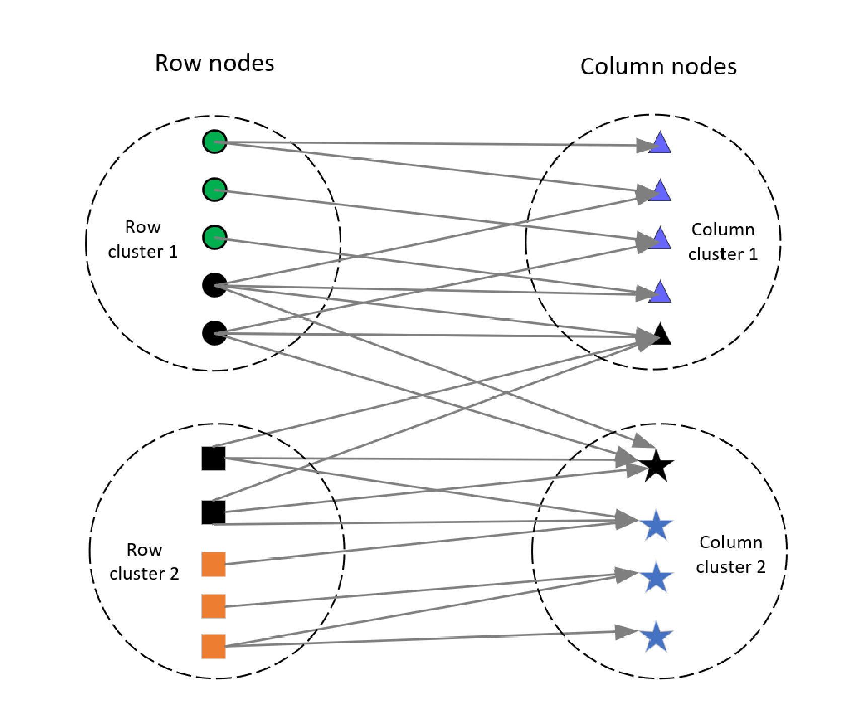
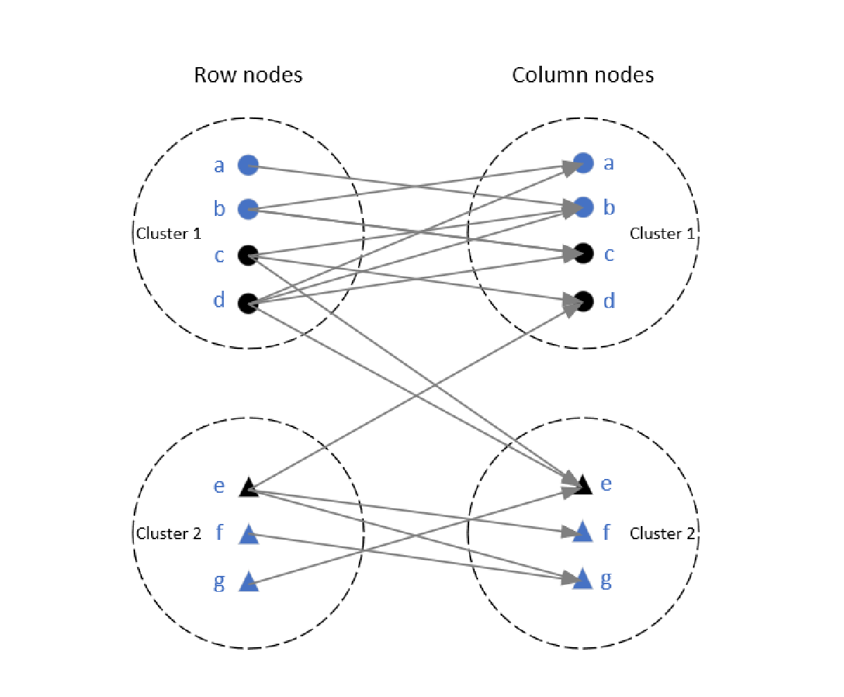
Figure 1: Two schematic diagrams for DiMMSB.

DiMMSB can model various networks, and the generality of DiMMSB can be laconically explained by the two schematic diagrams in Figure 1. In the figure, an arrow demonstrates a directed edge from one node to another, nodes in the same cluster are enclosed by dashed circle, and nodes in black have mixed memberships. In panel (a) of Figure 1, row nodes and column nodes are the same, 7 nodes in this network (i.e., A∈ℝ7×7A\in\mathbb{R}^{7\times 7}), nodes a,b,c,da,b,c,d belong to row cluster 1 and they also belong to column cluster 1, and nodes e,f,ge,f,g belong to row cluster 2 and column cluster 2. Since nodes cc and dd point to nodes ee, node ee points to node dd, these three nodes c,d,ec,d,e have mixed memberships. In panel (b), row nodes are different from column nodes. There are 10 row nodes where nodes referred by solid circle belong to row cluster 1, and nodes referred by solid square belong to row cluster 2. There are 9 column nodes where nodes referred by solid triangle belong to column cluster 1, and nodes referred by solid star belong to column cluster 2. The directed adjacency matrix AA in panel (b) is a 10×910\times 9 matrix, whose row nodes are different from column nodes. Meanwhile, for row nodes, since the black circles and the black squares point to the black triangle node and the black star node, they are mixed row nodes. Since the black triangle node and the black star node are pointed by mixed nodes, they are treated as mixed column nodes. Meanwhile, works in Rohe et al. 2016; Zhou and A.Amini 2019; Razaee et al. 2019; Zhou and Amini 2020; Ndaoud et al. 2021 also consider the general case when row nodes may differ column nodes for their theoretical analysis.

2.1 Identifiability

The parameters in the DiMMSB model obviously need to be constrained to guarantee identifiability of the model. All models with communities, are considered identifiable if they are identifiable up to a permutation of community labels Jin et al. 2017; Zhang et al. 2020; Mao et al. 2020. The following conditions are sufficient for the identifiability of DiMMSB:

  • •

    (I1) rank⁡(P)=K\mathrm{rank}(P)=K.

  • •

    (I2) There is at least one pure node for each of the KK row and KK column communities.

The full rank condition (I1) for connectivity matrix PP and pure nodes condition (I2) are popular conditions for models modeling network with mixed memberships, see Jin et al. 2017; Zhang et al. 2020; Mao et al. 2018; Mao et al. 2020. Now we decompose AA into a sum of a ‘signal’ part and a ‘noise’ part:

A=Ω+W,\displaystyle A=\Omega+W,

where the nr×ncn_{r}\times n_{c} matrix Ω\Omega is the expectation of the adjacency matrix AA, and WW is a generalized Wigner matrix. Then, under DiMMSB, we have

Ω=Πr​P​Πc′.\displaystyle\Omega=\Pi_{r}P\Pi_{c}^{\prime}. (7)

We refer Ω\Omega as the population adjacency matrix. By basic algebra, we know Ω\Omega is of rank KK. Thus Ω\Omega is a low-rank matrix (K<min⁡{nr,nc}K<\min\{n_{r},n_{c}\}) which is the key for why spectral clustering method works for DiMMSB.

Next proposition guarantees that when conditions (I1) and (I2) hold, DiMMSB is identifiable.

Proposition 1.

If conditions (I1) and (I2) hold, DiMMSB is identifiable, i.e., if a given matrix Ω\Omega corresponds to a set of parameters (nr,nc,K,P,Πr,Πc)(n_{r},n_{c},K,P,\Pi_{r},\Pi_{c}) through (7), these parameters are unique up to a permutation of community labels.

Unless specified, we treat conditions (I1) and (I2) as default from now on.

2.2 Sparsity scaling

Real-world large scale networks are usually sparse, in the sense that the number of edges from a node (the node degree) are very small compared to the total number of nodes. Generally speaking, community recovery is hard when the data set is sparse. As a result, an important criterion of evaluating a community recovery method is its performance under different levels of sparsity. In this paper, we capture the sparsity of a directed mixed membership network by the sparsity parameter ρ\rho such that

P=ρ​P~​where​max1≤k,l≤K​P~​(k,l)=1.\displaystyle P=\rho\tilde{P}\mathrm{~where~}\mathrm{max}_{1\leq k,l\leq K}\tilde{P}(k,l)=1.

Under D​i​M​M​S​B​(nr,nc,K,P,Πr,Πc)DiMMSB(n_{r},n_{c},K,P,\Pi_{r},\Pi_{c}), a smaller ρ\rho leads to a smaller probability to generate an edge from row node ii to column node jj, i.e., the sparsity parameter ρ\rho captures the sparsity behaviors for generating a directed mixed membership network. When building theoretical guarantee on estimation consistency of spectral clustering methods in community detection, controlling the sparsity of a network is common, see Lei and Rinaldo 2015; Jin 2015; Rohe et al. 2016; Mao et al. 2020; Wang et al. 2020. Especially, when DiMMSB degenerates to SBM, Assumption 1 matches the sparsity requirement in Theorem 3.1 Lei and Rinaldo 2015, and this guarantees the optimality of our sparsity condition. Meanwhile, as mentioned in Jin et al. 2017; Mao et al. 2020, σK​(P~)\sigma_{K}(\tilde{P}) is a measure of the separation between communities and a larger σK​(P~)\sigma_{K}(\tilde{P}) gives more well-separated communities. This paper also aims at studying the effect of ρ\rho and σK​(P~)\sigma_{K}(\tilde{P}) on the performance of spectral clustering by allowing them to be contained in the error bound. Therefore, our theoretical results allow model parameters K,ρ,σK​(P~)K,\rho,\sigma_{K}(\tilde{P}) to vary with nrn_{r} and ncn_{c}.

3 A spectral algorithm for fitting DiMMSB

The primary goal of the proposed algorithm is to estimate the row membership matrix Πr\Pi_{r} and column membership matrix Πc\Pi_{c} from the observed adjacency matrix AA with given KK. Considering the computational scalability, we focus on the idea of spectral clustering by spectral decomposition to design an efficient algorithm under DiMMSB in this paper.

We now discuss our intuition for the design of our algorithm. Under conditions (I1) and (I2), by basic algebra, we have rank⁡(Ω)=K\mathrm{rank}(\Omega)=K, which is much smaller than min​{nr,nc}\mathrm{min}\{n_{r},n_{c}\}. Let Ω=U​Λ​V′\Omega=U\Lambda V^{\prime} be the compact singular value decomposition (SVD) of Ω\Omega, where U∈ℝnr×K,Λ∈ℝK×K,V∈ℝnc×KU\in\mathbb{R}^{n_{r}\times K},\Lambda\in\mathbb{R}^{K\times K},V\in\mathbb{R}^{n_{c}\times K}, U′​U=IK,V′​V=IKU^{\prime}U=I_{K},V^{\prime}V=I_{K}, and IKI_{K} is a K×KK\times K identity matrix. For 1≤k≤K1\leq k\leq K, let ℐr(k)={i∈{1,2,…,nr}:Πr​(i,k)=1}\mathcal{I}^{(k)}_{r}=\{i\in\{1,2,\ldots,n_{r}\}:\Pi_{r}(i,k)=1\} and ℐc(k)={j∈{1,2,…,nc}:Πc​(j,k)=1}\mathcal{I}^{(k)}_{c}=\{j\in\{1,2,\ldots,n_{c}\}:\Pi_{c}(j,k)=1\}. By condition (I2), ℐr(k)\mathcal{I}^{(k)}_{r} and ℐc(k)\mathcal{I}^{(k)}_{c} are non empty for all 1≤k≤K1\leq k\leq K. For 1≤k≤K1\leq k\leq K, select one row node from ℐr(k)\mathcal{I}^{(k)}_{r} to construct the index set ℐr\mathcal{I}_{r}, i.e., ℐr\mathcal{I}_{r} is the indices of row nodes corresponding to KK pure row nodes, one from each community. And ℐc\mathcal{I}_{c} is defined similarly. W.L.O.G., let Πr(ℐr,:)=IK\Pi_{r}(\mathcal{I}_{r},:)=I_{K} and Πc(ℐc,:)=IK\Pi_{c}(\mathcal{I}_{c},:)=I_{K} (Lemma 2.1 in Mao et al. 2020 also has similar setting to design their spectral algorithms under MMSB.). The existences of the Row Ideal Simplex (RIS for short) structure inherent in UU and the Column Ideal Simplex (CIS for short) structure inherent in VV are guaranteed by the following lemma.

Lemma 1.

(Row Ideal Simplex and Column Ideal Simplex). Under D​i​M​M​S​B​(nr,nc,K,P,Πr,Πc)DiMMSB(n_{r},n_{c},K,P,\Pi_{r},\Pi_{c}), there exist an unique K×KK\times K matrix BrB_{r} and an unique K×KK\times K matrix BcB_{c} such that

  • •

    U=Πr​BrU=\Pi_{r}B_{r} where Br=U(ℐr,:)B_{r}=U(\mathcal{I}_{r},:). Meanwhile, U(i,:)=U(i¯,:)U(i,:)=U(\bar{i},:), if Πr(i,:)=Πr(i¯,:)\Pi_{r}(i,:)=\Pi_{r}(\bar{i},:) for 1≤i,i¯≤nr1\leq i,\bar{i}\leq n_{r}.

  • •

    V=Πc​BcV=\Pi_{c}B_{c} where Bc=V(ℐc,:)B_{c}=V(\mathcal{I}_{c},:). Meanwhile, V(j,:)=V(j¯,:)V(j,:)=V(\bar{j},:), if Πc(j,:)=Πc(j¯,:)\Pi_{c}(j,:)=\Pi_{c}(\bar{j},:) for 1≤j,j¯≤nc1\leq j,\bar{j}\leq n_{c}.

Lemma 1 says that the rows of UU form a KK-simplex in ℝK\mathbb{R}^{K} which we call the Row Ideal Simplex (RIS), with the KK rows of BrB_{r} being the vertices. Similarly, rows of VV form a KK-simplex in ℝK\mathbb{R}^{K} which we call the Column Ideal Simplex (CIS), with the KK rows of BcB_{c} being the vertices. Meanwhile, U(i,:)U(i,:) is a convex linear combination of Br(1,:),Br(2,:),…,Br(K,:)B_{r}(1,:),B_{r}(2,:),\ldots,B_{r}(K,:) for 1≤i≤nr1\leq i\leq n_{r}. If row node ii is pure, U(i,:)U(i,:) falls exactly on one of the vertices of the RIS. If row node ii is mixed, U(i,:)U(i,:) is in the interior or face of the RIS, but not on any of the vertices. Similar conclusions hold for column nodes.

Since BrB_{r} and BcB_{c} are full rank matrices, if U,V,BrU,V,B_{r} and BcB_{c} are known in advance ideally, we can exactly obtain Πr\Pi_{r} and Πc\Pi_{c} by setting Πr=U​Br′​(Br​Br′)−1\Pi_{r}=UB_{r}^{\prime}(B_{r}B_{r}^{\prime})^{-1} and Πc=V​Bc′​(Bc​Bc′)−1\Pi_{c}=VB_{c}^{\prime}(B_{c}B_{c}^{\prime})^{-1}.

While in practice, the estimation of U​Br′​(Br​Br′)−1UB_{r}^{\prime}(B_{r}B_{r}^{\prime})^{-1} and V​Bc′​(Bc​Bc′)−1VB_{c}^{\prime}(B_{c}B_{c}^{\prime})^{-1} may not have unit row norm, thus we need to make the following transformation: Set Yr=U​Br′​(Br​Br′)−1,Y_{r}=UB_{r}^{\prime}(B_{r}B_{r}^{\prime})^{-1}, and Yc=V​Bc′​(Bc​Bc′)−1Y_{c}=VB_{c}^{\prime}(B_{c}B_{c}^{\prime})^{-1}. Then the membership matrices can be estimated by

Πr(i,:)=Yr(i,:)∥Yr(i,:)∥1,Πc(j,:)=Yc(j,:)∥Yc(j,:)∥1,1≤i≤nr,1≤j≤nc.\displaystyle\Pi_{r}(i,:)=\frac{Y_{r}(i,:)}{\|Y_{r}(i,:)\|_{1}},\Pi_{c}(j,:)=\frac{Y_{c}(j,:)}{\|Y_{c}(j,:)\|_{1}},1\leq i\leq n_{r},1\leq j\leq n_{c}.

By the RIS structure U=ΠrBr≡ΠrU(ℐr,:)U=\Pi_{r}B_{r}\equiv\Pi_{r}U(\mathcal{I}_{r},:), as long as we can obtain the row corner matrix U(ℐr,:)U(\mathcal{I}_{r},:) (i.e., BrB_{r}), we can recover Πr\Pi_{r} exactly. As mentioned in Jin et al. 2017 and Mao et al. 2020, for such ideal simplex, the successive projection (SP) algorithm Gillis and Vavasis 2015 (for details of SP, see Algorithm 4) can be applied to UU with KK row communities to find BrB_{r}. The above analysis gives how to recover Πr\Pi_{r} with given Ω\Omega and KK under DiMMSB ideally. Similarly, Πc\Pi_{c} can be exactly recovered by applying SP on all rows of VV with KK column communities.

Based on the above analysis, we are now ready to give the following three-stage algorithm which we call Ideal DiSP. Input Ω\Omega and KK. Output: Πr\Pi_{r} and Πc\Pi_{c}.

  • •

    PCA step. Let Ω=U​Λ​V′\Omega=U\Lambda V^{\prime} be the compact SVD of Ω\Omega such that U∈ℝnr×K,V∈ℝnc×K,Λ∈ℝK×K,U′​U=I,V′​V=IU\in\mathbb{R}^{n_{r}\times K},V\in\mathbb{R}^{n_{c}\times K},\Lambda\in\mathbb{R}^{K\times K},U^{\prime}U=I,V^{\prime}V=I.

  • •

    Vertex Hunting (VH) step. Run SP algorithm on all rows of UU (and VV) assuming there are KK row (column) communities to obtain BrB_{r} (and BcB_{c}).

  • •

    Membership Reconstruction (MR) step. Set Yr=U​Br′​(Br​Br′)−1Y_{r}=UB_{r}^{\prime}(B_{r}B_{r}^{\prime})^{-1} and
    Yc=U​Bc′​(Bc​Bc′)−1Y_{c}=UB_{c}^{\prime}(B_{c}B_{c}^{\prime})^{-1}. Recover Πr\Pi_{r} and Πc\Pi_{c} by setting Πr(i,:)=Yr(i,:)∥Yr(i,:)∥1\Pi_{r}(i,:)=\frac{Y_{r}(i,:)}{\|Y_{r}(i,:)\|_{1}} for 1≤i≤nr1\leq i\leq n_{r}, and Πc(j,:)=Yc(j,:)∥Yc(j,:)∥1\Pi_{c}(j,:)=\frac{Y_{c}(j,:)}{\|Y_{c}(j,:)\|_{1}} for 1≤j≤nc1\leq j\leq n_{c}.

The following theorem guarantees that Ideal DiSP exactly recover nodes memberships and this also verifies the identifiability of DiMMSB in turn.

Theorem 1.

(Ideal DiSP). Under D​i​M​M​S​B​(nr,nc,K,P,Πr,Πc)DiMMSB(n_{r},n_{c},K,P,\Pi_{r},\Pi_{c}), the Ideal DiSP exactly recovers the row nodes membership matrix Πr\Pi_{r} and the column nodes membership matrix Πc\Pi_{c}.

We now extend the ideal case to the real case. Set A~=U^​Λ^​V^′\tilde{A}=\hat{U}\hat{\Lambda}\hat{V}^{\prime} be the top-KK-dimensional SVD of AA such that U^∈ℝnr×K,V^∈ℝnc×K,Λ^∈ℝK×K,U^′​U^=IK,V^′​V^=IK\hat{U}\in\mathbb{R}^{n_{r}\times K},\hat{V}\in\mathbb{R}^{n_{c}\times K},\hat{\Lambda}\in\mathbb{R}^{K\times K},\hat{U}^{\prime}\hat{U}=I_{K},\hat{V}^{\prime}\hat{V}=I_{K}, and Λ^\hat{\Lambda} contains the top KK singular values of AA. For the real case, we use B^r,B^c,Y^r,Y^c,Π^r,Π^c\hat{B}_{r},\hat{B}_{c},\hat{Y}_{r},\hat{Y}_{c},\hat{\Pi}_{r},\hat{\Pi}_{c} given in Algorithm 1 to estimate Br,Bc,Yr,Yc,Πr,ΠcB_{r},B_{c},Y_{r},Y_{c},\Pi_{r},\Pi_{c}, respectively. Algorithm 1 called DiSP is a natural extension of the Ideal DiSP to the real case.

Algorithm 1 DiSP
1: The adjacency matrix A∈ℝnr×ncA\in\mathbb{R}^{n_{r}\times n_{c}}, the number of row (column) communities KK.
2: The estimated nr×Kn_{r}\times K row membership matrix Π^r\hat{\Pi}_{r} and the estimated nc×Kn_{c}\times K column membership matrix Π^c\hat{\Pi}_{c}.
3: PCA step. Compute the left singular vectors U^∈ℝnr×K\hat{U}\in\mathbb{R}^{n_{r}\times K} and right singular vectors V^∈ℝnc×K\hat{V}\in\mathbb{R}^{n_{c}\times K} of AA.
4: Vertex Hunting (VH) step. Apply SP algorithm (i.e., Algorithm 4) on the rows of U^\hat{U} assuming there are KK row clusters to obtain the near-corners matrix U^(ℐ^r,:)∈ℝK×K\hat{U}(\mathcal{\hat{I}}_{r},:)\in\mathbb{R}^{K\times K}, where ℐ^r\mathcal{\hat{I}}_{r} is the index set returned by SP algorithm. Similarly, apply SP algorithm on the rows of V^\hat{V} with KK column clusters to obtain V^(ℐ^c,:)∈ℝK×K\hat{V}(\mathcal{\hat{I}}_{c},:)\in\mathbb{R}^{K\times K}, where ℐ^c\mathcal{\hat{I}}_{c} is the index set returned by SP algorithm. Set B^r=U^(ℐ^r,:),B^c=V^(ℐ^c,:)\hat{B}_{r}=\hat{U}(\mathcal{\hat{I}}_{r},:),\hat{B}_{c}=\hat{V}(\mathcal{\hat{I}}_{c},:).
5: Membership Reconstruction (MR) step. Compute the nr×Kn_{r}\times K matrix Y^r\hat{Y}_{r} such that Y^r=U^​B^r′​(B^r​B^r′)−1\hat{Y}_{r}=\hat{U}\hat{B}_{r}^{\prime}(\hat{B}_{r}\hat{B}_{r}^{\prime})^{-1}. Set Y^r=max⁡(0,Y^r)\hat{Y}_{r}=\mathrm{max}(0,\hat{Y}_{r}) and estimate Πr(i,:)\Pi_{r}(i,:) by Π^r(i,:)=Y^r(i,:)/∥Y^r(i,:)∥1,1≤i≤nr\hat{\Pi}_{r}(i,:)=\hat{Y}_{r}(i,:)/\|\hat{Y}_{r}(i,:)\|_{1},1\leq i\leq n_{r}. Similarly, compute the nc×Kn_{c}\times K matrix Y^c\hat{Y}_{c} such that Y^c=V^​B^c′​(B^c​B^c′)−1\hat{Y}_{c}=\hat{V}\hat{B}_{c}^{\prime}(\hat{B}_{c}\hat{B}_{c}^{\prime})^{-1}. Set Y^c=max⁡(0,Y^c)\hat{Y}_{c}=\mathrm{max}(0,\hat{Y}_{c}) and estimate Πc(j,:)\Pi_{c}(j,:) by Π^c(j,:)=Y^c(j,:)/∥Y^c(j,:)∥1,1≤j≤nc\hat{\Pi}_{c}(j,:)=\hat{Y}_{c}(j,:)/\|\hat{Y}_{c}(j,:)\|_{1},1\leq j\leq n_{c}.

In the MR step, we set the negative entries of Y^r\hat{Y}_{r} as 0 by setting Y^r=max⁡(0,Y^r)\hat{Y}_{r}=\mathrm{max}(0,\hat{Y}_{r}) for the reason that weights for any row node should be nonnegative while there may exist some negative entries of U^​B^r′​(B^r​B^r′)−1\hat{U}\hat{B}_{r}^{\prime}(\hat{B}_{r}\hat{B}_{r}^{\prime})^{-1}. Meanwhile, since B^r\hat{B}_{r} has KK distinct rows and nrn_{r} is always much lager than KK, the inverse of B^r​B^r′\hat{B}_{r}\hat{B}_{r}^{\prime} always exists in practice. Similar statements hold for column nodes.

Refer to caption
(a) UU
Refer to caption
(b) VV
Refer to caption
(c) U^\hat{U} when nr,0=60n_{r,0}=60
Refer to caption
(d) U^\hat{U} when nr,0=120n_{r,0}=120
Refer to caption
(e) U^\hat{U} when nr,0=180n_{r,0}=180
Refer to caption
(f) V^\hat{V} when nc,0=40n_{c,0}=40
Refer to caption
(g) V^\hat{V} when nc,0=100n_{c,0}=100
Refer to caption
(h) V^\hat{V} when nc,0=160n_{c,0}=160
Figure 2: Panel (a) shows the RIS in Experiment 4 when nc,0=nr,0=120n_{c,0}=n_{r,0}=120, where nc,0n_{c,0} and nr,0n_{r,0} are the numbers of pure nodes in row and column respectively (black: pure nodes; blue: mixed nodes. Each point is a row of UU. Many rows are equal, so a point may represent many rows). All mixed (both row and column) nodes evenly distributed in 4 groups, where the PMFs equal to (0.4,0.4,0.2),(0.4,0.2,0.4),(0.2,0.4,0.4)(0.4,0.4,0.2),(0.4,0.2,0.4),(0.2,0.4,0.4) and (1/3,1/3,1/3)(1/3,1/3,1/3). Panel (b) shows the CIS with same setting as (a). Panel (c): each point is a row of U^\hat{U} while black point is the vertex obtained by SP algorithm in Experiment 4 when setting nr,0=60n_{r,0}=60. Similar interpretations for Panels (d)-(h). Since K=3K=3 in Experiment 4, for visualization, we have projected and rotated these points from ℝ3\mathbb{R}^{3} to ℝ2\mathbb{R}^{2}.

To demonstrate the RIS and CIS, we drew Figure 2. Panel (a) supports that if row node ii is pure, then U(i,:)U(i,:) falls on the vertex of the RIS, otherwise U(i,:)U(i,:) falls in the interior of the RIS. Similar arguments hold for VV. In panels (c)-(h), we plot U^\hat{U} and V^\hat{V} under different settings of the number of pure nodes in row clusters and column clusters, where the data is generated by DiMMSB under the setting of Experiment 4. And in panels (c)-(h) of Figure 2, we also plot the B^r\hat{B}_{r} and B^c\hat{B}_{c}. From panels (c)-(e), we can find that points in U^\hat{U} generated from the same row cluster are always much closer than row nodes from different row clusters. Meanwhile, as the number of pure row nodes nr,0n_{r,0} increases for each row cluster, the number of points fall in the interior of the triangle decreases. Similar arguments hold for V^\hat{V}.

3.1 Equivalence algorithm

For the convenience of theoretical analysis, we introduce an equivalent algorithm DiSP-equivalence which returns same estimations as Algorithm 1 (see Remark 7 for details). Denote U2=U​U′∈ℝnr×nr,U^2=U^​U^′∈ℝnr×nr,V2=V​V′∈ℝnc×nc,V^2=V^​V^′∈ℝnc×ncU_{2}=UU^{\prime}\in\mathbb{R}^{n_{r}\times n_{r}},\hat{U}_{2}=\hat{U}\hat{U}^{\prime}\in\mathbb{R}^{n_{r}\times n_{r}},V_{2}=VV^{\prime}\in\mathbb{R}^{n_{c}\times n_{c}},\hat{V}_{2}=\hat{V}\hat{V}^{\prime}\in\mathbb{R}^{n_{c}\times n_{c}}. Next lemma guarantees that U2U_{2} and V2V_{2} have simplex structures.

Lemma 2.

Under D​i​M​M​S​B​(nr,nc,K,P,Πr,Πc)DiMMSB(n_{r},n_{c},K,P,\Pi_{r},\Pi_{c}), we have U2=ΠrU2(ℐr,:)U_{2}=\Pi_{r}U_{2}(\mathcal{I}_{r},:) and V2=ΠcV2(ℐc,:)V_{2}=\Pi_{c}V_{2}(\mathcal{I}_{c},:).

Since U2(ℐr,:)∈ℝK×nrU_{2}(\mathcal{I}_{r},:)\in\mathbb{R}^{K\times n_{r}} and V2(ℐc,:)∈ℝK×ncV_{2}(\mathcal{I}_{c},:)\in\mathbb{R}^{K\times n_{c}}, U2(ℐr,:)U_{2}(\mathcal{I}_{r},:) and V2(ℐc,:)V_{2}(\mathcal{I}_{c},:) are singular matrix with rank KK by condition (I1). Lemma 2 gives that

Πr=U2U2′(ℐr,:)(U2(ℐr,:)U2′(ℐr,:))−1,Πc=V2V2′(ℐc,:)(V2(ℐc,:)V2′(ℐc,:))−1.\displaystyle\Pi_{r}=U_{2}U^{\prime}_{2}(\mathcal{I}_{r},:)(U_{2}(\mathcal{I}_{r},:)U^{\prime}_{2}(\mathcal{I}_{r},:))^{-1},\Pi_{c}=V_{2}V^{\prime}_{2}(\mathcal{I}_{c},:)(V_{2}(\mathcal{I}_{c},:)V^{\prime}_{2}(\mathcal{I}_{c},:))^{-1}.

Based on the above analysis, we are now ready to give the Ideal DiSP-equivalence. Input Ω\Omega and KK. Output: Πr\Pi_{r} and Πc\Pi_{c}.

  • •

    PCA step. Obtain U2U_{2} and V2V_{2}.

  • •

    VH step. Apply SP algorithm on rows of U2U_{2} to obtain U2(ℐr,:)U_{2}(\mathcal{I}_{r},:) and on rows of V2V_{2} to obtain V2(ℐc,:)V_{2}(\mathcal{I}_{c},:) assuming there are KK row (column) communities.

  • •

    MR step. Recover Πr=U2U2′(ℐr,:)(U2(ℐr,:)U2′(ℐr,:))−1,Πc=V2V2′(ℐc,:)(V2(ℐc,:)V2′(ℐc,:))−1\Pi_{r}=U_{2}U^{\prime}_{2}(\mathcal{I}_{r},:)(U_{2}(\mathcal{I}_{r},:)U^{\prime}_{2}(\mathcal{I}_{r},:))^{-1},\Pi_{c}=V_{2}V^{\prime}_{2}(\mathcal{I}_{c},:)(V_{2}(\mathcal{I}_{c},:)V^{\prime}_{2}(\mathcal{I}_{c},:))^{-1}.

We now extend the ideal case to the real one as below.

Algorithm 2 DiSP-equivalence
1: The adjacency matrix A∈ℝnr×ncA\in\mathbb{R}^{n_{r}\times n_{c}}, the number of row (column) communities KK.
2: The estimated nr×Kn_{r}\times K row membership matrix Π^r,2\hat{\Pi}_{r,2} and the estimated nc×Kn_{c}\times K column membership matrix Π^c,2\hat{\Pi}_{c,2}.
3: PCA step. Compute U^2∈ℝnr×nr\hat{U}_{2}\in\mathbb{R}^{n_{r}\times n_{r}} and V^2∈ℝnc×nc\hat{V}_{2}\in\mathbb{R}^{n_{c}\times n_{c}} of AA.
4: VH step. Apply SP algorithm on U^2\hat{U}_{2} with KK row clusters to obtain U^2(ℐ^r,2,:)∈ℝK×nr\hat{U}_{2}(\hat{\mathcal{I}}_{r,2},:)\in\mathbb{R}^{K\times n_{r}} where ℐ^r,2\mathcal{\hat{I}}_{r,2} is the index set returned by SP algorithm. Similarly, apply SP algorithm on V^2\hat{V}_{2} with KK column clusters to obtain V^2(ℐ^c,2,:)∈ℝK×nc\hat{V}_{2}(\hat{\mathcal{I}}_{c,2},:)\in\mathbb{R}^{K\times n_{c}} where ℐ^c,2\mathcal{\hat{I}}_{c,2} is the index set returned by SP algorithm.
5: Membership Reconstruction (MR) step. Compute the nr×Kn_{r}\times K matrix Y^r,2\hat{Y}_{r,2} such that Y^r,2=U^2U^2′(ℐ^r,2,:)(U^2(ℐ^r,2,:)U^2′(ℐ^r,2,:))−1\hat{Y}_{r,2}=\hat{U}_{2}\hat{U}^{\prime}_{2}(\hat{\mathcal{I}}_{r,2},:)(\hat{U}_{2}(\hat{\mathcal{I}}_{r,2},:)\hat{U}^{\prime}_{2}(\hat{\mathcal{I}}_{r,2},:))^{-1}. Set Y^r,2=max⁡(0,Y^r,2)\hat{Y}_{r,2}=\mathrm{max}(0,\hat{Y}_{r,2}) and estimate Πr,2(i,:)\Pi_{r,2}(i,:) by Π^r,2(i,:)=Y^r,2(i,:)/∥Y^r,2(i,:)∥1,1≤i≤nr\hat{\Pi}_{r,2}(i,:)=\hat{Y}_{r,2}(i,:)/\|\hat{Y}_{r,2}(i,:)\|_{1},1\leq i\leq n_{r}. Similarly, compute the nc×Kn_{c}\times K matrix Y^c,2\hat{Y}_{c,2} such that Y^c,2=V^2V^2′(V^2(ℐ^c,2,:)V^2′(ℐ^c,2,:))−1\hat{Y}_{c,2}=\hat{V}_{2}\hat{V}^{\prime}_{2}(\hat{V}_{2}(\hat{\mathcal{I}}_{c,2},:)\hat{V}^{\prime}_{2}(\hat{\mathcal{I}}_{c,2},:))^{-1}. Set Y^c,2=max⁡(0,Y^c,2)\hat{Y}_{c,2}=\mathrm{max}(0,\hat{Y}_{c,2}) and estimate Πc,2(j,:)\Pi_{c,2}(j,:) by Π^c,2(j,:)=Y^c,2(j,:)/∥Y^c,2(j,:)∥1,1≤j≤nc\hat{\Pi}_{c,2}(j,:)=\hat{Y}_{c,2}(j,:)/\|\hat{Y}_{c,2}(j,:)\|_{1},1\leq j\leq n_{c}.

Lemma 3.2 in Mao et al. 2020 gives ℐ^r=ℐ^r,2\hat{\mathcal{I}}_{r}=\hat{\mathcal{I}}_{r,2} and ℐ^c=ℐ^c,2\hat{\mathcal{I}}_{c}=\hat{\mathcal{I}}_{c,2} (i.e., SP algorithm will return the same indices on both U^\hat{U} and U^2\hat{U}_{2} as well as V^\hat{V} and V^2\hat{V}_{2}), which gives that U^2U^2′(ℐ^r,2,:)=U^2U^2′(ℐ^r,:)=U^U^′((U^U^′)(ℐ^r,:))′=U^U^′(U^(ℐ^r,:)U^′)′=U^U^′U^U^′(ℐ^r,:)=U^U^′(ℐ^r,:)\hat{U}_{2}\hat{U}^{\prime}_{2}(\hat{\mathcal{I}}_{r,2},:)=\hat{U}_{2}\hat{U}^{\prime}_{2}(\hat{\mathcal{I}}_{r},:)=\hat{U}\hat{U}^{\prime}((\hat{U}\hat{U}^{\prime})(\hat{\mathcal{I}}_{r},:))^{\prime}=\hat{U}\hat{U}^{\prime}(\hat{U}(\hat{\mathcal{I}}_{r},:)\hat{U}^{\prime})^{\prime}=\hat{U}\hat{U}^{\prime}\hat{U}\hat{U}^{\prime}(\hat{\mathcal{I}}_{r},:)=\hat{U}\hat{U}^{\prime}(\hat{\mathcal{I}}_{r},:), and U^2(ℐ^r,2,:)U^2′(ℐ^r,2,:)=U^2(ℐ^r,:)U^2′(ℐ^r,:)=U^(ℐ^r,:)U^′(U^(ℐ^r,:)U^′)′=U^(ℐ^r,:)U^′(ℐ^r,:)\hat{U}_{2}(\hat{\mathcal{I}}_{r,2},:)\hat{U}^{\prime}_{2}(\hat{\mathcal{I}}_{r,2},:)=\hat{U}_{2}(\hat{\mathcal{I}}_{r},:)\hat{U}^{\prime}_{2}(\hat{\mathcal{I}}_{r},:)=\hat{U}(\hat{\mathcal{I}}_{r},:)\hat{U}^{\prime}(\hat{U}(\hat{\mathcal{I}}_{r},:)\hat{U}^{\prime})^{\prime}=\hat{U}(\hat{\mathcal{I}}_{r},:)\hat{U}^{\prime}(\hat{\mathcal{I}}_{r},:). Therefore, Y^r,2=Y^r,Π^r,2=Π^r\hat{Y}_{r,2}=\hat{Y}_{r},\hat{\Pi}_{r,2}=\hat{\Pi}_{r}. Following similar analysis, we also have Y^c,2=Y^c,\hat{Y}_{c,2}=\hat{Y}_{c}, and Π^c,2=Π^c\hat{\Pi}_{c,2}=\hat{\Pi}_{c}. Hence, the above analysis guarantees that the two algorithms 1 and 2 return same estimations for both row and column nodes’s memberships.

4 Main results for DiSP

In this section, we show the consistency of our algorithm, i.e., to show that the sample-based estimates Π^r\hat{\Pi}_{r} and Π^c\hat{\Pi}_{c} concentrate around the true mixed membership matrix Πr\Pi_{r} and Πc\Pi_{c}. Throughout this paper, KK is a known positive integer.

First, we bound ‖A−Ω‖\|A-\Omega\| based on the application of the rectangular version of Bernstein inequality in Tropp 2012. This technique allows us to deal with rectangular random matrices, and it is the corner stone for that our algorithm DiSP can fit DiMMSB when nr≠ncn_{r}\neq n_{c}. We assume that

Assumption 1.

ρ​max​(nr,nc)≥log⁡(nr+nc).\rho\mathrm{max}(n_{r},n_{c})\geq\mathrm{log}(n_{r}+n_{c}).

Assumption 1 means that the network can not be too sparse. Then we have the following lemma.

Lemma 3.

Under D​i​M​M​S​B​(nr,nc,K,P,Πr,Πc)DiMMSB(n_{r},n_{c},K,P,\Pi_{r},\Pi_{c}), when Assumption 1 holds, with probability at least 1−o⁡((nr+nc)−α)1-o((n_{r}+n_{c})^{-\alpha}) for any α>0\alpha>0, we have

‖A−Ω‖=O⁡(ρ​max​(nr,nc)​log​(nr+nc)).\displaystyle\|A-\Omega\|=O(\sqrt{\rho\mathrm{max}(n_{r},n_{c})\mathrm{log}(n_{r}+n_{c})}).

Then we can obtain the row-wise deviation bound for the singular eigenvectors of Ω\Omega.

Lemma 4.

(Row-wise singular eigenvector error) Under D​i​M​M​S​B​(nr,nc,K,P,Πr,Πc)DiMMSB(n_{r},n_{c},K,P,\Pi_{r},\Pi_{c}), when Assumption 1 holds, suppose σK​(Ω)≥C​ρ⁡(nr+nc)​log​(nr+nc)\sigma_{K}(\Omega)\geq C\sqrt{\rho(n_{r}+n_{c})\mathrm{log}(n_{r}+n_{c})}, with probability at least 1−o⁡((nr+nc)−α)1-o((n_{r}+n_{c})^{-\alpha}), we have

max⁡(‖U^​U^′−U​U′‖2→∞,‖V^​V^′−V​V′‖2→∞)=O⁡(K​(κ​(Ω)​max⁡(nr,nc)​μmin⁡(nr,nc)+log⁡(nr+nc))ρ​σK​(P~)​σK​(Πr)​σK​(Πc)),\displaystyle\mathrm{max}(\|\hat{U}\hat{U}^{\prime}-UU^{\prime}\|_{2\rightarrow\infty},\|\hat{V}\hat{V}^{\prime}-VV^{\prime}\|_{2\rightarrow\infty})=O(\frac{\sqrt{K}(\kappa(\Omega)\sqrt{\frac{\mathrm{max}(n_{r},n_{c})\mu}{\mathrm{min}(n_{r},n_{c})}}+\sqrt{\mathrm{log}(n_{r}+n_{c})})}{\sqrt{\rho}\sigma_{K}(\tilde{P})\sigma_{K}(\Pi_{r})\sigma_{K}(\Pi_{c})}),

where μ\mu is the incoherence parameter defined as μ=max⁡(nr​‖U‖2→∞2K,nc​‖V‖2→∞2K)\mu=\mathrm{max}(\frac{n_{r}\|U\|^{2}_{2\rightarrow\infty}}{K},\frac{n_{c}\|V\|^{2}_{2\rightarrow\infty}}{K}).

For convenience, set ϖ=max⁡(‖U^​U^′−U​U′‖2→∞,‖V^​V^′−V​V′‖2→∞)\varpi=\mathrm{max}(\|\hat{U}\hat{U}^{\prime}-UU^{\prime}\|_{2\rightarrow\infty},\|\hat{V}\hat{V}^{\prime}-VV^{\prime}\|_{2\rightarrow\infty}). When nr=nc=nn_{r}=n_{c}=n and Πr=Πc=Π\Pi_{r}=\Pi_{c}=\Pi, DiMMSB degenerates to MMSB. If we further assume that λK​(Π′​Π)=O⁡(nK)\lambda_{K}(\Pi^{\prime}\Pi)=O(\frac{n}{K}) and K=O⁡(1)K=O(1), the bound in Lemma 4 can be simplified as O⁡(1σK​(P~)​1n​log⁡(n)ρ​n)O(\frac{1}{\sigma_{K}(\tilde{P})}\frac{1}{\sqrt{n}}\sqrt{\frac{\mathrm{log}(n)}{\rho n}}). This simplified form is consistent with the Lemma 2.1 in Jin et al. 2017. In detail, by setting the Θ\Theta in Jin et al. 2017 as ρ​I\sqrt{\rho}I to degenerate their DCMM to MMSB, and translating their assumptions to λK​(Π′​Π)=O⁡(nK)\lambda_{K}(\Pi^{\prime}\Pi)=O(\frac{n}{K}), when K=O⁡(1)K=O(1), the row-wise deviation bound in the fourth bullet of Lemma 2.1 in Jin et al. 2017 is the same as our reduced bound. Then if we further assume that σK​(P~)=O​(1)\sigma_{K}(\tilde{P})=O(1), the bound is of order 1n​log⁡(n)ρ​n\frac{1}{\sqrt{n}}\sqrt{\frac{\mathrm{log}(n)}{\rho n}}, which is consistent with the row-wise eigenvector deviation of Lei 2019’s result shown in their Table 2.

Next we bound the vertex centers matrix obtained by SP algorithm.

Lemma 5.

Under D​i​M​M​S​B​(nr,nc,K,P,Πr,Πc)DiMMSB(n_{r},n_{c},K,P,\Pi_{r},\Pi_{c}), when conditions in Lemma 4 hold, there exist two permutation matrices 𝒫r,𝒫c∈ℝK×K\mathcal{P}_{r},\mathcal{P}_{c}\in\mathbb{R}^{K\times K} such that with probability at least 1−o⁡((nr+nc)−α)1-o((n_{r}+n_{c})^{-\alpha}), we have

max1≤k≤K∥ek′(U^2(ℐ^r,:)−𝒫r′U2(ℐr,:))∥F=O(ϖκ(Πr′Πr)),\displaystyle\mathrm{max}_{1\leq k\leq K}\|e^{\prime}_{k}(\hat{U}_{2}(\mathcal{\hat{I}}_{r},:)-\mathcal{P}^{\prime}_{r}U_{2}(\mathcal{I}_{r},:))\|_{F}=O(\varpi\kappa(\Pi^{\prime}_{r}\Pi_{r})),
max1≤k≤K∥ek′(V^2(ℐ^c,:)−𝒫c′V2(ℐc,:))∥F=O(ϖκ(Πc′Πc)).\displaystyle\mathrm{max}_{1\leq k\leq K}\|e^{\prime}_{k}(\hat{V}_{2}(\mathcal{\hat{I}}_{c},:)-\mathcal{P}^{\prime}_{c}V_{2}(\mathcal{I}_{c},:))\|_{F}=O(\varpi\kappa(\Pi^{\prime}_{c}\Pi_{c})).
Lemma 6.

Under D​i​M​M​S​B​(nr,nc,K,P,Πr,Πc)DiMMSB(n_{r},n_{c},K,P,\Pi_{r},\Pi_{c}), when conditions in Lemma 4 hold,, with probability at least 1−o⁡((nr+nc)−α)1-o((n_{r}+n_{c})^{-\alpha}), for 1≤i≤nr,1≤j≤nc1\leq i\leq n_{r},1\leq j\leq n_{c}, we have

‖ei′​(Y^r−Yr​𝒫r)‖F=O⁡(ϖ​κ​(Πr′​Πr)​K​λ1​(Πr′​Πr)),‖ej′​(Y^c−Yc​𝒫c)‖F=O⁡(ϖ​κ​(Πc′​Πc)​K​λ1​(Πc′​Πc)).\displaystyle\|e^{\prime}_{i}(\hat{Y}_{r}-Y_{r}\mathcal{P}_{r})\|_{F}=O(\varpi\kappa(\Pi^{\prime}_{r}\Pi_{r})\sqrt{K\lambda_{1}(\Pi^{\prime}_{r}\Pi_{r})}),\|e^{\prime}_{j}(\hat{Y}_{c}-Y_{c}\mathcal{P}_{c})\|_{F}=O(\varpi\kappa(\Pi^{\prime}_{c}\Pi_{c})\sqrt{K\lambda_{1}(\Pi^{\prime}_{c}\Pi_{c})}).

Next theorem gives theoretical bounds on estimations of memberships for both row and column nodes, which is the main theoretical result for our DiSP method.

Theorem 2.

Under D​i​M​M​S​B​(nr,nc,K,P,Πr,Πc)DiMMSB(n_{r},n_{c},K,P,\Pi_{r},\Pi_{c}), suppose conditions in Lemma 4 hold, with probability at least 1−o⁡((nr+nc)−α)1-o((n_{r}+n_{c})^{-\alpha}), for 1≤i≤nr,1≤j≤nc1\leq i\leq n_{r},1\leq j\leq n_{c}, we have

‖ei′​(Π^r−Πr​𝒫r)‖1=O⁡(ϖ​κ​(Πr′​Πr)​K​λ1​(Πr′​Πr)),\displaystyle\|e^{\prime}_{i}(\hat{\Pi}_{r}-\Pi_{r}\mathcal{P}_{r})\|_{1}=O(\varpi\kappa(\Pi^{\prime}_{r}\Pi_{r})K\sqrt{\lambda_{1}(\Pi^{\prime}_{r}\Pi_{r})}),
‖ej′​(Π^c−Πc​𝒫c)‖1=O⁡(ϖ​κ​(Πc′​Πc)​K​λ1​(Πc′​Πc)).\displaystyle\|e^{\prime}_{j}(\hat{\Pi}_{c}-\Pi_{c}\mathcal{P}_{c})\|_{1}=O(\varpi\kappa(\Pi^{\prime}_{c}\Pi_{c})K\sqrt{\lambda_{1}(\Pi^{\prime}_{c}\Pi_{c})}).

Similar as Corollary 3.1 in Mao et al. 2020, by considering more conditions, we have the following corollary.

Corollary 1.

Under D​i​M​M​S​B​(nr,nc,K,P,Πr,Πc)DiMMSB(n_{r},n_{c},K,P,\Pi_{r},\Pi_{c}), when conditions in Lemma 4 hold, suppose λK​(Πr′​Πr)=O⁡(nrK)\lambda_{K}(\Pi^{\prime}_{r}\Pi_{r})=O(\frac{n_{r}}{K}) and λK​(Πc′​Πc)=O⁡(ncK)\lambda_{K}(\Pi^{\prime}_{c}\Pi_{c})=O(\frac{n_{c}}{K}), with probability at least 1−o⁡((nr+nc)−α)1-o((n_{r}+n_{c})^{-\alpha}), for 1≤i≤nr,1≤j≤nc1\leq i\leq n_{r},1\leq j\leq n_{c}, we have

‖ei′​(Π^r−Πr​𝒫r)‖1=O⁡(K2​(C​max⁡(nr,nc)min⁡(nr,nc)+log⁡(nr+nc))σK​(P~)​ρ​nc),\displaystyle\|e^{\prime}_{i}(\hat{\Pi}_{r}-\Pi_{r}\mathcal{P}_{r})\|_{1}=O(\frac{K^{2}(\sqrt{C\frac{\mathrm{max}(n_{r},n_{c})}{\mathrm{min}(n_{r},n_{c})}}+\sqrt{\mathrm{log}(n_{r}+n_{c})})}{\sigma_{K}(\tilde{P})\sqrt{\rho n_{c}}}),
‖ej′​(Π^c−Πc​𝒫c)‖1=O⁡(K2​(C​max⁡(nr,nc)min⁡(nr,nc)+log⁡(nr+nc))σK​(P~)​ρ​nr),\displaystyle\|e^{\prime}_{j}(\hat{\Pi}_{c}-\Pi_{c}\mathcal{P}_{c})\|_{1}=O(\frac{K^{2}(\sqrt{C\frac{\mathrm{max}(n_{r},n_{c})}{\mathrm{min}(n_{r},n_{c})}}+\sqrt{\mathrm{log}(n_{r}+n_{c})})}{\sigma_{K}(\tilde{P})\sqrt{\rho n_{r}}}),

where CC is a positive constant. Meanwhile,

  • •

    when C​max⁡(nr,nc)min⁡(nr,nc)≤log⁡(nr+nc)C\frac{\mathrm{max}(n_{r},n_{c})}{\mathrm{min}(n_{r},n_{c})}\leq\mathrm{log}(n_{r}+n_{c}), we have

    ‖ei′​(Π^r−Πr​𝒫r)‖1=O⁡(K2​log⁡(nr+nc)σK​(P~)​ρ​nc),‖ej′​(Π^c−Πc​𝒫c)‖1=O⁡(K2​log⁡(nr+nc)σK​(P~)​ρ​nr).\displaystyle\|e^{\prime}_{i}(\hat{\Pi}_{r}-\Pi_{r}\mathcal{P}_{r})\|_{1}=O(\frac{K^{2}\sqrt{\mathrm{log}(n_{r}+n_{c})}}{\sigma_{K}(\tilde{P})\sqrt{\rho n_{c}}}),\|e^{\prime}_{j}(\hat{\Pi}_{c}-\Pi_{c}\mathcal{P}_{c})\|_{1}=O(\frac{K^{2}\sqrt{\mathrm{log}(n_{r}+n_{c})}}{\sigma_{K}(\tilde{P})\sqrt{\rho n_{r}}}).
  • •

    when nr=O⁡(n),nc=O⁡(n)n_{r}=O(n),n_{c}=O(n) (i.e., nrnc=O⁡(1)\frac{n_{r}}{n_{c}}=O(1)), we have

    ‖ei′​(Π^r−Πr​𝒫r)‖1=O⁡(K2σK​(P~)​log⁡(n)ρ​n),‖ej′​(Π^c−Πc​𝒫c)‖1=O⁡(K2σK​(P~)​log⁡(n)ρ​n).\displaystyle\|e^{\prime}_{i}(\hat{\Pi}_{r}-\Pi_{r}\mathcal{P}_{r})\|_{1}=O(\frac{K^{2}}{\sigma_{K}(\tilde{P})}\sqrt{\frac{\mathrm{log}(n)}{\rho n}}),\|e^{\prime}_{j}(\hat{\Pi}_{c}-\Pi_{c}\mathcal{P}_{c})\|_{1}=O(\frac{K^{2}}{\sigma_{K}(\tilde{P})}\sqrt{\frac{\mathrm{log}(n)}{\rho n}}).

Under the settings of Corollary 1, when K=O⁡(1)K=O(1), to ensure the consistency of estimation, for the case C​max⁡(nr,nc)min⁡(nr,nc)≤log⁡(nr+nc)C\frac{\mathrm{max}(n_{r},n_{c})}{\mathrm{min}(n_{r},n_{c})}\leq\mathrm{log}(n_{r}+n_{c}), σK​(P~)\sigma_{K}(\tilde{P}) should shrink slower than log⁡(nr+nc)ρ​min​(nr+nc)\sqrt{\frac{\mathrm{log}(n_{r}+n_{c})}{\rho\mathrm{min}(n_{r}+n_{c})}}; Similarly, for the case nrnc=O⁡(1)\frac{n_{r}}{n_{c}}=O(1), σK​(P~)\sigma_{K}(\tilde{P}) should shrink slower than log⁡(n)ρ​n\sqrt{\frac{\mathrm{log}(n)}{\rho n}}.

Remark 1.

By Lemma 10, we know σK​(Ω)≥ρ​σK​(P~)​σK​(Πr)​σK​(Πc)\sigma_{K}(\Omega)\geq\rho\sigma_{K}(\tilde{P})\sigma_{K}(\Pi_{r})\sigma_{K}(\Pi_{c}). To ensure the condition σK​(Ω)≥C​(ρ⁡(nr+nc)​log​(nr+nc))1/2\sigma_{K}(\Omega)\geq C(\rho(n_{r}+n_{c})\mathrm{log}(n_{r}+n_{c}))^{1/2} in lemma 4 hold, we need ρ​σK​(P~)​σK​(Πr)​σK​(Πc)≥C​(ρ⁡(nr+nc)​log​(nr+nc))1/2\rho\sigma_{K}(\tilde{P})\sigma_{K}(\Pi_{r})\sigma_{K}(\Pi_{c})\geq C(\rho(n_{r}+n_{c})\mathrm{log}(n_{r}+n_{c}))^{1/2}. Thus

σK​(P~)≥C​((nr+nc)​log​(nr+nc)ρ​λK​(Πr′​Πr)​λK​(Πc′​Πc))1/2.\displaystyle\sigma_{K}(\tilde{P})\geq C\big(\frac{(n_{r}+n_{c})\mathrm{log}(n_{r}+n_{c})}{\rho\lambda_{K}(\Pi^{\prime}_{r}\Pi_{r})\lambda_{K}(\Pi^{\prime}_{c}\Pi_{c})}\big)^{1/2}. (8)

When K=O⁡(1),λK​(Πr′​Πr)=O⁡(nrK),K=O(1),\lambda_{K}(\Pi^{\prime}_{r}\Pi_{r})=O(\frac{n_{r}}{K}), and λK​(Πc′​Πc)=O⁡(ncK)\lambda_{K}(\Pi^{\prime}_{c}\Pi_{c})=O(\frac{n_{c}}{K}), Eq (8) gives that σK​(P~)\sigma_{K}(\tilde{P}) should grow faster than log1/2​(nr+nc)/(ρ​min​(nr,nc))1/2\mathrm{log}^{1/2}(n_{r}+n_{c})/(\rho\mathrm{min}(n_{r},n_{c}))^{1/2}, which matches with the consistency requirement on σK​(P~)\sigma_{K}(\tilde{P}) obtained from Corollary 1.

Remark 2.

When DiMMSB degenerates to MMSB, for the network with nr=nc=nn_{r}=n_{c}=n and K=O⁡(1)K=O(1), the upper bound of error rate for DiSP is O⁡(1σK​(P~)​log⁡(n)ρ​n)O(\frac{1}{\sigma_{K}(\tilde{P})}\sqrt{\frac{\mathrm{log}(n)}{\rho n}}). Replacing the Θ\Theta in Jin et al. 2017 by Θ=ρ​I\Theta=\sqrt{\rho}I, their DCMM model degenerates to the MMSB. Then their conditions in Theorem 2.2 are the same as our assumption (1) and λK​(Π′​Π)=O⁡(nK)\lambda_{K}(\Pi^{\prime}\Pi)=O(\frac{n}{K}) where Π=Πr=Πc\Pi=\Pi_{r}=\Pi_{c} for MMSB. When K=O⁡(1)K=O(1), the error bound in Theorem 2.2 in Jin et al. 2017 is O⁡(1|λK​(P~)|​log⁡(n)ρ​n)O(\frac{1}{|\lambda_{K}(\tilde{P})|}\sqrt{\frac{\mathrm{log}(n)}{\rho n}}), which is consistent with ours since |λK​(P~)|=σK​(P~)|\lambda_{K}(\tilde{P})|=\sigma_{K}(\tilde{P}). This guarantees the optimality of our theoretical results.

Similarly, under the settings of Corollary 1, for the case C​max⁡(nr,nc)min⁡(nr,nc)≤log⁡(nr+nc)C\frac{\mathrm{max}(n_{r},n_{c})}{\mathrm{min}(n_{r},n_{c})}\leq\mathrm{log}(n_{r}+n_{c}), when σK​(P~)\sigma_{K}(\tilde{P}) is a constant, the upper bounds of error rates for both row clusters and column clusters are O⁡(K2​log⁡(nr+nc)ρ​min​(nr,nc))O(K^{2}\sqrt{\frac{\mathrm{log}(n_{r}+n_{c})}{\rho\mathrm{min}(n_{r},n_{c})}}). Therefore, for consistent estimation of DiSP, KK should grow slower than (ρ​min​(nr+nc)log⁡(nr+nc))1/4(\frac{\rho\mathrm{min}(n_{r}+n_{c})}{\mathrm{log}(n_{r}+n_{c})})^{1/4}. Similarly, under the settings of Corollary 1, for the case nrnc=O⁡(1)\frac{n_{r}}{n_{c}}=O(1), when σK​(P~)\sigma_{K}(\tilde{P}) is a constant, the upper bounds of error rates are O⁡(K2​log⁡(n)ρ​n)O(K^{2}\sqrt{\frac{\mathrm{log}(n)}{\rho n}}). For consistent estimation, KK should grow slower than (ρ​nlog⁡(n))1/4(\frac{\rho n}{\mathrm{log}(n)})^{1/4}.

Consider the balanced directed mixed membership network (i.e., λK​(Πr′​Πr)=O⁡(nrK),λK​(Πc′​Πc)=O⁡(ncK)\lambda_{K}(\Pi^{\prime}_{r}\Pi_{r})=O(\frac{n_{r}}{K}),\lambda_{K}(\Pi^{\prime}_{c}\Pi_{c})=O(\frac{n_{c}}{K}) and nr=O⁡(n),nc=O⁡(n)n_{r}=O(n),n_{c}=O(n)) in Corollary 1, we further assume that P~=β​IK+(1−β)​1K​1K′\tilde{P}=\beta I_{K}+(1-\beta)\textbf{1}_{K}\textbf{1}^{\prime}_{K} (where 1K\textbf{1}_{K} is a K×1K\times 1 vector with all entries being ones.) for 0<β<10<\beta<1 when K=O⁡(1)K=O(1) and call such directed network as standard directed mixed membership network. To obtain consistency estimation, β\beta should shrink slower than log⁡(n)ρ​n\sqrt{\frac{\mathrm{log}(n)}{\rho n}} since σK​(P~)=β\sigma_{K}(\tilde{P})=\beta. Let Pmax=maxk,l⁡P⁡(k,l),Pmin=mink,l​P​(k,l)P_{\mathrm{max}}=\max_{k,l}P(k,l),P_{\mathrm{min}}=\mathrm{min}_{k,l}P(k,l). Since P=ρ​P~P=\rho\tilde{P} , we have Pmax−Pmin=ρ​βP_{\mathrm{max}}-P_{\mathrm{min}}=\rho\beta (the probability gap) should shrink slower than ρ​log​(n)n\sqrt{\frac{\rho\mathrm{log}(n)}{n}} and Pmax−PminPmax=β​ρ\frac{P_{\mathrm{max}}-P_{\mathrm{min}}}{\sqrt{P_{\mathrm{max}}}}=\beta\sqrt{\rho} (the relative edge probability gap) should shrink slower than log⁡(n)n\sqrt{\frac{\mathrm{log}(n)}{n}}. Especially, for the sparest network ρ​n=log⁡(n)\rho n=\mathrm{log}(n) satisfying assumption (1), the probability gap should shrink slower than log⁡(n)n\frac{\mathrm{log}(n)}{n}.

5 Simulations

In this section, some simulations are conducted to investigate the performance of our DiSP. We measure the performance of the proposed method by Di-Mixed-Hamming error rate, row-Mixed-Hamming error rate and column-Mixed-Hamming error rate, and they are defined as:

  • •

    DiMHamm=min𝒫∈S​‖Π^r​𝒫−Πr‖1+min𝒫∈S​‖Π^c​𝒫​Πc‖1nr+nc=\frac{\mathrm{min}_{\mathcal{P}\in S}\|\hat{\Pi}_{r}\mathcal{P}-\Pi_{r}\|_{1}+\mathrm{min}_{\mathcal{P}\in S}\|\hat{\Pi}_{c}\mathcal{P}\Pi_{c}\|_{1}}{n_{r}+n_{c}},

  • •

    row-MHamm=min𝒫∈S​‖Π^r​𝒫−Πr‖1nr=\frac{\mathrm{min}_{\mathcal{P}\in S}\|\hat{\Pi}_{r}\mathcal{P}-\Pi_{r}\|_{1}}{n_{r}},

  • •

    column-MHamm=min𝒫∈S​‖Π^c​𝒫−Πc‖1nc=\frac{\mathrm{min}_{\mathcal{P}\in S}\|\hat{\Pi}_{c}\mathcal{P}-\Pi_{c}\|_{1}}{n_{c}},

where Πr​(Πc)\Pi_{r}~(\Pi_{c}) and Π^r​(Π^c)\hat{\Pi}_{r}~(\hat{\Pi}_{c}) are the true and estimated row (column) mixed membership matrices respectively, and SS is the set of K×KK\times K permutation matrices. Here, we also consider the permutation of labels since the measurement of error should not depend on how we label each of the K communities. DiMHamm is used to measure the DiSP’s performances on both row nodes and column nodes, while row-MHamm and column-MHamm are used to measure its performance on row nodes and column nodes respectively. Meanwhile, in the following 1-3 experiments, we compare DiSP with the variational expectation-maximization (vEM for short) algorithm Airoldi et al. 2013 for their two-way stochastic blockmodels with Bernoulli distribution. By Table 1 in Airoldi et al. 2013, we see that vEM under the two input Dirichlet parameters α=0.05,β=0.05\alpha=0.05,\beta=0.05 (by Airoldi et al. 2013’s notation) generally performs better than that under α=β=0.2\alpha=\beta=0.2. Therefore, in our simulations, we set the two Dirichlet parameters α\alpha and β\beta of vEM as 0.050.05.

For the first three simulations in this section, unless specified, the parameters (nr,nc,K,P,Πr,Πc)(n_{r},n_{c},K,P,\Pi_{r},\Pi_{c}) under DiMMSB are set as follows. For row nodes, nr=60n_{r}=60 and K=3K=3. Let each row block own nr,0n_{r,0} number of pure nodes. We let the top K​nr,0Kn_{r,0} row nodes {1,2,…,K​nr,0}\{1,2,\ldots,Kn_{r,0}\} be pure and the rest row nodes {K​nr,0+1,K​nr,0+2,…,nr}\{Kn_{r,0}+1,Kn_{r,0}+2,\ldots,n_{r}\} be mixed. Unless specified, let all the mixed row nodes have four different memberships (0.4,0.4,0.2),(0.4,0.2,0.4),(0.2,0.4,0.4)(0.4,0.4,0.2),(0.4,0.2,0.4),(0.2,0.4,0.4) and (1/3,1/3,1/3)(1/3,1/3,1/3), each with nr−K​nr,04\frac{n_{r}-Kn_{r,0}}{4} number of nodes when K=3K=3. For column nodes, set nc=80n_{c}=80. Let each column block own nc,0n_{c,0} number of pure nodes. Let the top K​nc,0Kn_{c,0} column nodes {1,2,…,K​nc,0}\{1,2,\ldots,Kn_{c,0}\} be pure and column nodes {K​nc,0+1,K​nc,0+2,…,nc}\{Kn_{c,0}+1,Kn_{c,0}+2,\ldots,n_{c}\} be mixed. The settings of column mixed memberships are same as row mixed memberships. When nr,0=nc,0n_{r,0}=n_{c,0}, denote n0=nr,0=nc,0n_{0}=n_{r,0}=n_{c,0} for convenience. The probability matrix PP is set independently for each experiment.

After obtaining P,Πr,ΠcP,\Pi_{r},\Pi_{c}, similar as the five simulation steps in Jin 2015, each simulation experiment contains the following steps:

(a) Set Ω=Πr​P​Πc′\Omega=\Pi_{r}P\Pi^{\prime}_{c}.

(b) Let WW be an nr×ncn_{r}\times n_{c} matrix such that W⁡(i,j)W(i,j) are independent centered-Bernoulli with parameters Ω⁡(i,j)\Omega(i,j). Let A~=Ω+W\tilde{A}=\Omega+W.

(c) Set S~r={i:∑j=1ncA~​(i,j)=0}\tilde{S}_{r}=\{i:\sum_{j=1}^{n_{c}}\tilde{A}(i,j)=0\} and S~c={j:∑i=1nrA~​(i,j)=0}\tilde{S}_{c}=\{j:\sum_{i=1}^{n_{r}}\tilde{A}(i,j)=0\}, i.e., S~r\tilde{S}_{r} (S~c\tilde{S}_{c}) is the set of row (column) nodes with 0 edges. Let AA be the adjacency matrix obtained by removing rows respective to nodes in S~r\tilde{S}_{r} and removing columns respective to nodes in S~c\tilde{S}_{c} from A~\tilde{A}. Similarly, update Πr\Pi_{r} by removing nodes in S~r\tilde{S}_{r} and update Πc\Pi_{c} by removing nodes in S~c\tilde{S}_{c}.

(d) Apply DiSP (and vEM) algorithm to AA. Record DiMHamm, row-MHamm, column-MHamm and running time under investigations.

(e) Repeat (b)-(d) for 50 times, and report the averaged DiMHamm, averaged row-MHamm, averaged column-MHamm and averaged running time over the 50 repetitions.

In our experiments, the number of rows of AA and the number of columns of AA are usually very close to nrn_{r} and ncn_{c}, therefore we do not report the exact values of the the number of rows and columns of AA .

Refer to caption
(a) Changing n0n_{0}: DiMHamm
Refer to caption
(b) Changing n0n_{0}: row-MHamm
Refer to caption
(c) Changing n0n_{0}:column-MHamm
Refer to caption
(d) Changing ρ\rho: DiMHamm
Refer to caption
(e) Changing ρ\rho: row-MHamm
Refer to caption
(f) Changing ρ\rho: column-MHamm
Refer to caption
(g) Changing β\beta: DiMHamm
Refer to caption
(h) Changing β\beta: row-MHamm
Refer to caption
(i) Changing β\beta: column-MHamm
Refer to caption
(j) Changing n0n_{0}: run-time
Refer to caption
(k) Changing ρ\rho: run-time
Refer to caption
(l) Changing β\beta: run-time
Figure 3: Numerical results of Experiments 1-3.

Experiment 1: Changing n0n_{0}. The probability matrix in this experiment is set as

P=[0.80.10.30.20.90.40.50.20.9].P=\begin{bmatrix}0.8&0.1&0.3\\ 0.2&0.9&0.4\\ 0.5&0.2&0.9\\ \end{bmatrix}.

Let n0n_{0} range in {4,8,12,16,20}\{4,8,12,16,20\}. A larger n0n_{0} indicates a case with higher fraction of pure nodes for both row clusters and column clusters. The numerical results of error rates are shown in Panels (a), (b) and (c) of Figure 3. From the three panels, we see that the three error rates look similar, and the fraction of pure nodes influences the performance of DiSP and vEM such that the two methods perform better with the increasing number of pure nodes in the simulated network. The plots of run-time are shown in panel (j) of Figure 3. Meanwhile, codes for all numerical results in this paper are written in MATLAB R2021b. The total run-time of Experiment 1 for vEM is roughly 8 hours, and it is roughly 1.5 seconds for DiSP. Sure, DiSP outperforms vEM on both error rates and run-time.

Experiment 2: Changing ρ\rho. Let the sparsity parameter ρ∈{0.1,0.2,…,1}\rho\in\{0.1,0.2,\ldots,1\}. The probability matrix in this experiment is set as

P=ρ​[10.40.40.6110.20.20.4].P=\rho\begin{bmatrix}1&0.4&0.4\\ 0.6&1&1\\ 0.2&0.2&0.4\\ \end{bmatrix}.

A larger ρ\rho indicates a denser simulated network. Here, PP is set much different as that in Experiment 1, because we aim to emphasize that DiMMSB has no strict constraints on PP as long as rank⁡(P)=K\mathrm{rank}(P)=K and all elements of PP are in [0,1][0,1]. Panels (d), (e) and (f) in Figure 3 display simulation results of this experiment and panel (k) records run-time. Meanwhile, the total run-time of Experiment 2 for vEM is roughly 16 hours, and it is roughly 3.44 seconds for DiSP. From these results, we see that DiSP outperforms vEM on DiMHamm, column-MHamm and run-time while vEM performs better than DiSP on row-MHamm.

Experiment 3: Changing β\beta. Let β∈{0.1,0.2,…,1}\beta\in\{0.1,0.2,\ldots,1\}. The probability matrix in this experiment is set as

P=[11−β1−β1−β11−β1−β1−β1].P=\begin{bmatrix}1&1-\beta&1-\beta\\ 1-\beta&1&1-\beta\\ 1-\beta&1-\beta&1\\ \end{bmatrix}.

Since σK​(P)=β\sigma_{K}(P)=\beta, increasing β\beta decreases error rates by the analysis for the balanced directed mixed membership network. Panels (g), (h) and (i) in Figure 3 display simulation results of this experiment and panel (l) records run-time. These three error rates are similar in this experiment. Meanwhile, the total run-time of Experiment 2 for vEM is roughly 16 hours, and it is roughly 2.9 seconds for DiSP. We see that, DiSP outperforms vEM on both error rates and run-time.

Remark 3.

For visuality, we plot AA generated under DiMMSB. Let nr=24,nc=30,K=2n_{r}=24,n_{c}=30,K=2, and

P=[0.80.050.10.7].P=\begin{bmatrix}0.8&0.05&\\ 0.1&0.7\\ \end{bmatrix}.

For row nodes, let Πr​(i,1)=1\Pi_{r}(i,1)=1 for 1≤i≤81\leq i\leq 8, Πr​(i,2)=1\Pi_{r}(i,2)=1 for 9≤i≤169\leq i\leq 16, and Πr(i,:)=[0.70.3]\Pi_{r}(i,:)=[0.7~~0.3] for 17≤i≤2417\leq i\leq 24 (i.e., there are 16 pure row nodes and 8 mixed row nodes). For column nodes, let Πc​(i,1)=1\Pi_{c}(i,1)=1 for 1≤i≤81\leq i\leq 8, Πc​(i,2)=1\Pi_{c}(i,2)=1 for 9≤i≤169\leq i\leq 16, and Πc(i,:)=[0.70.3]\Pi_{c}(i,:)=[0.7~~0.3] for 17≤i≤3017\leq i\leq 30 (i.e., there are 16 pure column nodes and 14 mixed column nodes). For above setting, we generate two random adjacency matrices in Figure 4 where we also report error rates and run-time of DiSP and vEM. Here, because AA is provided in Figure 4, and Πr,Πc\Pi_{r},\Pi_{c} and KK are known. readers can apply DiSP to AA in Figure 4 to check the effectiveness of the proposed algorithm.

Refer to caption
Refer to caption
Figure 4: For adjacency matrix in panel (a),DiMHamm,row−MHamm\mathrm{~DiMHamm},\mathrm{~row-MHamm},column−MHamm\mathrm{~column-MHamm} and run-time for DiSP (vEM) are 0.0948 (0.1674),0.1070 (0.1384), 0.0849 (0.0948) and 0.0021(3.7988), respectively. For adjacency matrix in panel (b),DiMHamm,row−MHamm\mathrm{~DiMHamm},\mathrm{~row-MHamm},column−MHamm\mathrm{~column-MHamm} and run-time for DiSP (vEM) are 0.0778 (0.1745),0.0643 (0.1290), 0.0886 (0.2109) and 0.0020 (5.3025) seconds, respectively. x-axis: row nodes; y-axis: column nodes.
Remark 4.

For visuality, we also plot a directed network generated under DiMMSB. Let nr=24,nc=24,K=2n_{r}=24,n_{c}=24,K=2, and

P=0.8​[10.10.20.6].P=0.8\begin{bmatrix}1&0.1\\ 0.2&0.6\\ \end{bmatrix}.

For row nodes, let Πr​(i,1)=1\Pi_{r}(i,1)=1 for 1≤i≤81\leq i\leq 8, Πr​(i,2)=1\Pi_{r}(i,2)=1 for 9≤i≤169\leq i\leq 16, and Πr(i,:)=[0.70.3]\Pi_{r}(i,:)=[0.7~~0.3] for 17≤i≤2417\leq i\leq 24 (i.e., there are 16 pure row nodes and 8 mixed row nodes). For column nodes, let Πc​(i,1)=1\Pi_{c}(i,1)=1 for 1≤i≤101\leq i\leq 10, Πc​(i,2)=1\Pi_{c}(i,2)=1 for 11≤i≤2011\leq i\leq 20, and Πc(i,:)=[0.70.3]\Pi_{c}(i,:)=[0.7~~0.3] for 21≤i≤2421\leq i\leq 24 (i.e., there are 20 pure column nodes and 4 mixed column nodes). For above setting, we generate one AA in panel (a) and (b) of Figure 5 and panels (b) and (c) of Figure 5 show the sending pattern side and receiving pattern side of this simulated directed network, respectively.

Refer to caption
(a) Adjacency matrix
Refer to caption
(b) Sending clusters
Refer to caption
(c) Receiving clusters
Figure 5: Illustration of a simulated directed network generated under DiMMSB. Panels (a), (b) and (c) show AA, the sending clusters and the receiving clusters of this simulated directed network, respectively. For this directed network, DiMHamm,row−MHamm\mathrm{~DiMHamm},\mathrm{~row-MHamm},column−MHamm\mathrm{~column-MHamm} and run-time for DiSP (vEM) are 0.0796 (0.0956),0.0786 (0.1340), 0.0806 (0.0572) and 0.0021 (2.5566) seconds, respectively. In panels (b) and (c), colors indicate clusters and square indicates mixed nodes, where the sending and receiving clusters are obtained by Πr\Pi_{r} and Πc\Pi_{c} given in Remark 4. x-axis: row nodes; y-axis: column nodes.

In Experiments 1-3, we mainly investigate the performances of DiSP by comparing it with vEM on small directed mixed membership networks. The numerical results show that DiSP performs much better than vEM on error rates, and DiSP is much faster than vEM. However, the error rates are always quite large in Experiments 1-3 because the directed mixed membership network with 60 row nodes and 80 column nodes is too small and a few edges can be generated for such small directed mixed membership network under the settings in Experiments 1-3. In next four experiments, we investigate the performances of DiSP on some larger (compared with those under Experiments 1-3) directed mixed membership networks. Because the run-time for vEM is too large for large network, we do not compare DiSP with vEM in next four experiments.

Refer to caption
(a) Changing n0n_{0}: DiMHamm
Refer to caption
(b) Changing n0n_{0}: row-MHamm
Refer to caption
(c) Changing n0n_{0}: column-MHamm
Refer to caption
(d) Changing ρ\rho: DiMHamm
Refer to caption
(e) Changing ρ\rho: row-MHamm
Refer to caption
(f) Changing ρ\rho: column-MHamm
Refer to caption
(g) Changing β\beta: DiMHamm
Refer to caption
(h) Changing β\beta: row-MHamm
Refer to caption
(i) Changing β\beta: column-MHamm
Refer to caption
(j) Changing KK: DiMHamm
Refer to caption
(k) Changing KK: row-MHamm
Refer to caption
(l) Changing KK: column-MHamm
Refer to caption
(m) Changing n0n_{0}: run-time
Refer to caption
(n) Changing ρ\rho: run-time
Refer to caption
(o) Changing β\beta: run-time
Refer to caption
(p) Changing KK: run-time
Figure 6: Numerical results of Experiments 4-7.

Experiment 4: Changing n0n_{0}. Let nr=600,nc=800n_{r}=600,n_{c}=800, n0n_{0} range in {40,60,…,200}\{40,60,\ldots,200\}, and all other parameters are set the same as Experiment 1. Panels (a), (b) and (c) of Figure 6 record the error rates of DiSP in Experiment 4, and panel (m) records the run-time. The total run-time for Experiment 4 is roughly 36 seconds. We see that as the fraction of pure nodes increases, error rates decreases. Meanwhile, since size of network is much larger than network in Experiment 1, error rates in Experiment 4 are much smaller than that of Experiment 1 (similar conclusions hold for Experiments 5-6).

Experiment 5: Changing ρ\rho. Let nr=600,nc=800,n0=120n_{r}=600,n_{c}=800,n_{0}=120 and all other parameters are set the same as Experiment 2. Panels (d), (e) and (f) of Figure 6 record the error rates of DiSP in Experiment 5, and panel (n) records the run-time. The total run-time for Experiment 5 is roughly 55 seconds. We see that as ρ\rho increases, error rates tends to decrease.

Experiment 6: Changing β\beta. Let nr=600,nc=800,n0=120n_{r}=600,n_{c}=800,n_{0}=120 and all other parameters are set the same as Experiment 3. Panels (g), (h) and (i) of Figure 6 record the error rates of DiSP in Experiment 6, and panel (o) records the run-time. The total run-time for Experiment 6 is roughly 40.6 seconds. We see that as β\beta increases, error rates decreases, and this is consistent with the theoretical results in the last paragraph of Section 4.

Experiment 7: Changing KK. Let nr=1200,nc=1600,n_{r}=1200,n_{c}=1600, and n0=120n_{0}=120. Set diagonal elements, upper triangular elements and lower triangular elements of PP as 0.5, 0.2, 0.3, respectively. KK is varied in the range {2,3,…,8}\{2,3,\ldots,8\}. For the nr−K​n0n_{r}-Kn_{0} mixed row nodes and the nc−K​n0n_{c}-Kn_{0} mixed column nodes, let them belong to each block with equal probability 1K\frac{1}{K}. Panels (j), (k) and (l) of Figure 6 record the error rates of DiSP in Experiment 7, and panel (p) records the run-time. The total run-time for Experiment 7 is roughly 407 seconds. From the numerical results, we see that as KK increases, error rates increases first and then decreases. This phenomenon occurs since nrn_{r} and ncn_{c} are fixed, for a small KK, the fraction of pure row (column) nodes 120​K1200\frac{120K}{1200} (120​K1600\frac{120K}{1600} for column node) is small while the fraction of mixed row (column) nodes is large. As KK increases in this experiment, the fraction of pure row (column) nodes increases, and this is the reason that the proposed method performs better as KK increases when K≥6K\geq 6.

6 Applications to real-world data sets

For real-world directed networks considered in this paper, row nodes are always same as column nodes, so we have nr=nc=nn_{r}=n_{c}=n. Set dr​(i)=∑j=1nA⁡(i,j)d_{r}(i)=\sum_{j=1}^{n}A(i,j) as the sending side degree of node ii, and dc​(i)=∑j=1nA⁡(j,i)d_{c}(i)=\sum_{j=1}^{n}A(j,i) as the receiving side degree of node ii. We find that there exist many nodes with zero degree in real-world directed networks. Before applying our DiSP on adjacency matrix of real-world directed network, we need to pre-process the original directed network by Algorithm 3.

Algorithm 3 Pre-processing
1: Real-world directed network 𝒩\mathcal{N}.
2: Set A0A_{0} as the adjacency matrix of the original directed network 𝒩\mathcal{N}.
3: Find the row nodes set in which row nodes have zero degree by setting Sr,0={i:∑j=1nA0​(i,j)=0}S_{r,0}=\{i:\sum_{j=1}^{n}A_{0}(i,j)=0\}. For column nodes, set Sc,0={i:∑j=1nA0​(j,i)=0}S_{c,0}=\{i:\sum_{j=1}^{n}A_{0}(j,i)=0\}.
4: Set S0=Sr,0​⋃Sc,0S_{0}=S_{r,0}\bigcup S_{c,0}
5: Update A0A_{0} by setting A0=A0​(S0,S0)A_{0}=A_{0}(S_{0},S_{0}).
6: Repeat step 1 and step 2 until all nodes in S0S_{0} is null set.
7: Set AA as the largest connected component of A0A_{0}.

After pre-processing, we let Π^r\hat{\Pi}_{r} and Π^c\hat{\Pi}_{c} obtained from applying DiSP on AA with nn nodes and KK row (column) communities. Let ℓ^r\hat{\ell}_{r} be an n×1n\times 1 vector such that ℓ^r​(i)=argmax1≤k≤K​Π^r​(i,k)\hat{\ell}_{r}(i)=\mathrm{argmax}_{1\leq k\leq K}\hat{\Pi}_{r}(i,k), where ℓ^r​(i)\hat{\ell}_{r}(i) is called the home base row community of node ii. ℓ^c\hat{\ell}_{c} is defined similarly by setting ℓ^c​(i)=argmax1≤k≤K​Π^c​(i,k)\hat{\ell}_{c}(i)=\mathrm{argmax}_{1\leq k\leq K}\hat{\Pi}_{c}(i,k). We also need below statistics to investigate the directed network.

  • •

    Fraction of estimated highly mixed row (column) nodes: For row node ii, we treat it as a highly mixed row node if max1≤k≤K​Π^​(i,k)≤0.8\mathrm{max}_{1\leq k\leq K}\hat{\Pi}(i,k)\leq 0.8. Let τr\tau_{r} be the proportion of highly mixed row nodes such that τr=|{i:max1≤k≤K​Π^r​(i,k)≤0.8}|n\tau_{r}=\frac{|\{i:\mathrm{max}_{1\leq k\leq K}\hat{\Pi}_{r}(i,k)\leq 0.8\}|}{n}. Let τc\tau_{c} be the proportion of highly mixed column nodes such that τc=|{i:max1≤k≤K​Π^c​(i,k)≤0.8}|n\tau_{c}=\frac{|\{i:\mathrm{max}_{1\leq k\leq K}\hat{\Pi}_{c}(i,k)\leq 0.8\}|}{n}.

  • •

    The measurement of asymmetric structure between row clusters and column clusters: Since row nodes and column nodes are the same, to see whether the structure of row clusters differs from the structure of column clusters, we use the mixed-Hamming error rate computed as

    MHamm=minO∈S​‖Π^r​O−Π^c‖1n.\displaystyle\mathrm{MHamm}=\frac{\mathrm{min}_{O\in S}\|\hat{\Pi}_{r}O-\hat{\Pi}_{c}\|_{1}}{n}.

    We see that a larger (or a smaller) MHamm\mathrm{MHamm} indicates a heavy (slight) asymmetric between row communities and column communities.

We are now ready to describe some real-world directed networks as below:
Poltical blogs: this data was collected at 2004 US presidential election Adamic and Glance 2005. Such political blogs data can be represented by a directed graph, in which each node in the graph corresponds to a web blog labelled either as liberal or conservative (i.e., K=2K=2 for this data). An directed edge from node ii to node jj indicates that there is a hyperlink from blog ii to blog jj. Clearly, such a political blog graph is directed due to the fact that there is a hyperlink from blog ii to jj does not imply there is also a hyperlink from blog jj to ii. This data can be downloaded from http://www-personal.umich.edu/~mejn/netdata/. The original data has 1490 nodes, after pre-processing by Algorithm 3, A∈{0,1}813,813A\in\{0,1\}^{813,813}.
Human proteins (Stelzl): this network can be downloaded from http://konect.cc/networks/maayan-Stelzl and it represents interacting pairs of protein in Humans (Homo sapiens) Stelzl et al. 2005. In this data, node means protein and edge means interaction. The original data has 1706 nodes, after pre-processing, A∈{0,1}1507×1507A\in\{0,1\}^{1507\times 1507}. The number of row (column) clusters is unknown, to estimate it, we plot the leading 20 singular values of AA in panel (b) of Figure 7 and find that the eigengap suggests K=2K=2. Meanwhile, Rohe et al. 2016 also uses the idea of eigengap to choose KK for directed networks.
Wikipedia links (crh): this data represents the wikilinks of the Wikipedia in the Crimean Turkish language (crh), and it can be downloaded from http://konect.cc/networks/wikipedia_link_crh/. In this network, node denotes article, and edge denotes wikilink Kunegis 2013. After pro-processing, there are 3555 nodes, i.e., A∈{0,1}3555×3555A\in\{0,1\}^{3555\times 3555}. Panel (c) of Figure 7 suggests K=2K=2 for this data.
Wikipedia links (dv): this data consists of the wikilinks of the Wikipedia in the Divehi language (dv) where nodes are Wikipedia articles, and directed edges are wikilinks Kunegis 2013. It can be downloaded from http://konect.cc/networks/wikipedia_link_dv/. After pre-processing, A∈{0,1}2394×2394A\in\{0,1\}^{2394\times 2394}. K=2K=2 for this data. Panel (d) of Figure 7 suggests K=2K=2 for this data.

Refer to caption
(a) Political blogs
Refer to caption
(b) Human proteins (Stelzl)
Refer to caption
(c) Wikipedia links (crh)
Refer to caption
(d) Wikipedia links (dv)
Figure 7: Leading 20 singular values of adjacency matrices for real world directed networks used in this paper.

After obtaining AA and KK for real-world directed networks analyzed in this paper, we apply our DiSP to AA, and report τr,τc\tau_{r},\tau_{c} and MHamm\mathrm{MHamm} in Table 1. The results show that there is a slight asymmetric structure between row and column clusters for Poltical blogs, Human proteins (Stelzl) and Wikipedia links (crh) networks, because their MHamm\mathrm{MHamm} is small, while row clusters differs a lot from column clusters for Wikipedia links (dv) for its large MHamm\mathrm{MHamm}. For Poltical blogs, there exist 813×0.0246≈20813\times 0.0246\approx 20 highly mixed nodes in the sending pattern side while there exist 813×0.1353≈110813\times 0.1353\approx 110 highly mixed nodes in the receiving pattern side. For Human proteins (Stelzl), it has 1507×0.2986≈4501507\times 0.2986\approx 450 (and 1507×0.2999≈4521507\times 0.2999\approx 452) highly mixed nodes in the sending (receiving) pattern side. For Wikipedia links (crh), there are 3555×0.0444≈1583555\times 0.0444\approx 158 (and 3555×0.1308≈4653555\times 0.1308\approx 465)highly mixed nodes in the sending (receiving) pattern side. For Wikipedia links (dv), it has a large proportion of highly mixed nodes in both sending and receiving pattern side. Meanwhile, for visualization, we plot the sending clusters and receiving clusters detected by DiSP for real-world directed networks used in this paper in Figure 8, where we also mark the highly mixed nodes by sauare. Generally, we see that DiSP is useful in finding the highly mixed nodes and studying the asymmetric structure between row and column clusters of a directed network.

Table 1: The proportion of highly mixed nodes and the asymmetric structure measured by MHamm\mathrm{MHamm} for real world directed networks used in this paper by applying DiSP to their adjacency matrices assuming that there are K=2K=2 row (column) communities.
data τr\tau_{r} τc\tau_{c} MHamm\mathrm{MHamm}
Political blogs 0.0246 0.1353 0.0901
Human proteins (Stelzl) 0.2986 0.2999 0.0115
Wikipedia links (crh) 0.0444 0.1308 0.0643
Wikipedia links (dv) 0.4089 0.3008 0.1804
Refer to caption
(a) Political blogs
Refer to caption
(b) Political blogs
Refer to caption
(c) Human proteins (Stelzl)
Refer to caption
(d) Human proteins (Stelzl)
Refer to caption
(e) Wikipedia links (crh)
Refer to caption
(f) Wikipedia links (crh)
Refer to caption
(g) Wikipedia links (dv)
Refer to caption
(h) Wikipedia links (dv)
Figure 8: Sending and receiving clusters detected by DiSP for directed networks considered in this paper. Colors indicate clusters and square indicates highly mixed nodes, where sending and receiving clusters are obtained by ℓ^r\hat{\ell}_{r} and ℓ^c\hat{\ell}_{c}, respectively.

7 Discussions

In this paper, we introduce a directed mixed membership stochastic blockmodel to model directed network with mixed memberships. DiMMSB allows that both row and column nodes have mixed memberships, but the numbers of row nodes and column nodes could be different. We propose a spectral algorithm DiSP based on the SVD, SP algorithm and membership reconstruction skills. The theoretical results of DiSP show that DiSP can consistently recover memberships of both row nodes and column nodes under mild conditions. Meanwhile, we also obtain the separation conditions of a standard directed mixed membership network. When DiMMSB degenerates to MMSB, our theoretical results match that of Theorem 2.2 Jin et al. 2017 when their DCMM degenerates to MMSB under mild conditions. Through the applications on some real-world directed networks, DiSP finds the highly mixed nodes, and it also reveals new insights on the asymmetries in the structure of these directed networks. The model DiMMSB developed in this paper is useful to model directed networks and generate directed mixed membership networks with true background membership matrices. The proposed algorithm DiSP designed is useful in studying the asymmetric structure between sending and receiving clusters for a directed network. We expect that the model DiMMSB and the algorithm DiSP will have applications beyond this paper and can be widely applied to study the properties of directed networks in network science.

Acknowledgements

The authors would like to thank Dr. Edoardo M. Airoldi and Dr. Xiaopei Wang for sharing codes of vEM Airoldi et al. 2013 with us.

Appendix A Proof for identifiability

A.1 Proof of Proposition 1

Proof.

To proof the identifiability, we follow similar idea as the proof of (a) in Theorem 2.1 Mao et al. 2020 which provides the proof of identifiability of MMSB. Let Ω=U​Λ​V′\Omega=U\Lambda V^{\prime} be the compact singular value decomposition of Ω\Omega. By Lemma 1, U=Πr​Br,V=Πc​BcU=\Pi_{r}B_{r},V=\Pi_{c}B_{c}. Thus, for any node ii, U(i,:)U(i,:) lies in the convex hull of the KK rows of BrB_{r}, i.e., U(i,:)⊆Conv(Br)U(i,:)\subseteq\mathrm{Conv}(B_{r}) for 1≤i≤nr1\leq i\leq n_{r}. Similarly, we have V(j,:)⊆Conv(Bc)V(j,:)\subseteq\mathrm{Conv}(B_{c}) for 1≤j≤nc1\leq j\leq n_{c}, where we use Conv⁡(M)\mathrm{Conv}(M) denote the convex hull of the rows of the matrix MM.

Now, if Ω\Omega can be generated by another set of parameters (Π~r,P~,Π~c)(\tilde{\Pi}_{r},\tilde{P},\tilde{\Pi}_{c}) (i.e., Ω=Πr​P​Πc′=Π~r​P~​Π~c′\Omega=\Pi_{r}P\Pi_{c}^{\prime}=\tilde{\Pi}_{r}\tilde{P}\tilde{\Pi}_{c}^{\prime}), where Π~r\tilde{\Pi}_{r} and Π~c\tilde{\Pi}_{c} have different pure nodes sets, with indices ℐ~r≠1:K,ℐ~c≠1:K\tilde{\mathcal{I}}_{r}\neq 1:K,\tilde{\mathcal{I}}_{c}\neq 1:K. By the previous argument, we have U(ℐ~r,:)⊆Conv(Br)U(\tilde{\mathcal{I}}_{r},:)\subseteq\mathrm{Conv}(B_{r}) and V(ℐ~c,:)⊆Conv(Bc)V(\tilde{\mathcal{I}}_{c},:)\subseteq\mathrm{Conv}(B_{c}). Since (Πr,P,Πc)(\Pi_{r},P,\Pi_{c}) and (Π~r,P~,Π~c)(\tilde{\Pi}_{r},\tilde{P},\tilde{\Pi}_{c}) generate the same Ω\Omega, they have the same compact singular value decomposition up to a permutation of communities. Thus, swapping the roles of Πr\Pi_{r} and Π~r\tilde{\Pi}_{r}, and reapplying the above argument, we have Br⊆Conv(U(ℐ~r,:))B_{r}\subseteq\mathrm{Conv}(U(\tilde{\mathcal{I}}_{r},:)). Then Conv(Br)⊆Conv(U(ℐ~r,:))⊆Conv(Br)\mathrm{Conv}(B_{r})\subseteq\mathrm{Conv}(U(\tilde{\mathcal{I}}_{r},:))\subseteq\mathrm{Conv}(B_{r}), therefore we must have Conv(Br)=Conv(U(ℐ~r,:))\mathrm{Conv}(B_{r})=\mathrm{Conv}(U(\tilde{\mathcal{I}}_{r},:)). This means that pure nodes in Πr\Pi_{r} and Π~r\tilde{\Pi}_{r} are aligned up to a permutation, i.e., U(ℐ~r,:)=MrBrU(\tilde{\mathcal{I}}_{r},:)=M_{r}B_{r}, where Mr∈ℝK×KM_{r}\in\mathbb{R}^{K\times K} is a permutation matrix. Similarly, we have V(ℐ~c,:)=McBcV(\tilde{\mathcal{I}}_{c},:)=M_{c}B_{c}, where Mc∈ℝK×KM_{c}\in\mathbb{R}^{K\times K} is a permutation matrix.

By Lemma 1, we have U=Πr​BrU=\Pi_{r}B_{r} and U=Π~rU(ℐ~r,:)U=\tilde{\Pi}_{r}U(\tilde{\mathcal{I}}_{r},:), combining with U(ℐ~r,:)=MrBrU(\tilde{\mathcal{I}}_{r},:)=M_{r}B_{r}, we have

(Πr−Π~r​Mr)​Br=0.\displaystyle(\Pi_{r}-\tilde{\Pi}_{r}M_{r})B_{r}=0.

Since rank⁡(P)=K\mathrm{rank}(P)=K based on Condition (I1), we have rank⁡(Br)=K\mathrm{rank}(B_{r})=K, i.e., BrB_{r} is full rank. So we have Πr=Π~r​Mr\Pi_{r}=\tilde{\Pi}_{r}M_{r}. Thus, Πr\Pi_{r} and Π~r\tilde{\Pi}_{r} are identical up to a permutation. Similarly, Πc=Π~c​Mc\Pi_{c}=\tilde{\Pi}_{c}M_{c}, i.e., Πc\Pi_{c} and Π~c\tilde{\Pi}_{c} are identical up to a permutation. To have the same Ω\Omega, we have

Πr​P​Πc′\displaystyle\Pi_{r}P\Pi_{c}^{\prime} =Π~r​P~​Π~c′\displaystyle=\tilde{\Pi}_{r}\tilde{P}\tilde{\Pi}_{c}^{\prime}
⇓\displaystyle\Downarrow
Π~r​Mr​P​(Π~c​Mc)′\displaystyle\tilde{\Pi}_{r}M_{r}P(\tilde{\Pi}_{c}M_{c})^{\prime} =Π~r​P~​Π~c′\displaystyle=\tilde{\Pi}_{r}\tilde{P}\tilde{\Pi}_{c}^{\prime}
⇓\displaystyle\Downarrow
Mr​P​Mc′\displaystyle M_{r}PM_{c}^{\prime} =P~,\displaystyle=\tilde{P},

where the last equality holds by Lemma 7 and condition (I2). Mr​P​Mc′=P~M_{r}PM_{c}^{\prime}=\tilde{P} gives that PP and P~\tilde{P} are identical up to a row permutation and a column permutation.

Lemma 7.

For any membership matrix Π∈ℝn×K\Pi\in\mathbb{R}^{n\times K} whose ii-th row [Π⁡(i,1),Π⁡(i,2),…,Π⁡(i,K)][\Pi(i,1),\Pi(i,2),\ldots,\Pi(i,K)] is the PMF of node ii for 1≤i≤n1\leq i\leq n, such that each community has at least one pure node, then for any X,X~∈ℝK×KX,\tilde{X}\in\mathbb{R}^{K\times K}, if Π​X=Π​X~\Pi X=\Pi\tilde{X}, we have X=X~X=\tilde{X}.

Proof.

Assume that node ii is a pure node such that Π⁡(i,k)=1\Pi(i,k)=1, then the ii-th row of Π​X\Pi X is [X⁡(k,1),X⁡(k,2),…,X⁡(k,K)][X(k,1),X(k,2),\ldots,X(k,K)] (i.e., the ii-th row of Π​X\Pi X is the kk-th row of XX if Π⁡(i,k)=1\Pi(i,k)=1); similarly, the ii-th row of Π​X~\Pi\tilde{X} is the kk-th row of X~\tilde{X}. Since Π​X=Π​X~\Pi X=\Pi\tilde{X}, we have [X⁡(k,1),X⁡(k,2),…,X⁡(k,K)]=[X~​(k,1),X~​(k,2),…,X~​(k,K)][X(k,1),X(k,2),\ldots,X(k,K)]=[\tilde{X}(k,1),\tilde{X}(k,2),\ldots,\tilde{X}(k,K)] for 1≤k≤K1\leq k\leq K, hence X=X~X=\tilde{X}. ∎

Remark 5.

Here, we propose an alternative proof of DiMMSB’s identifiability. As in the main text, we always set Πr(ℐr,:)=IK\Pi_{r}(\mathcal{I}_{r},:)=I_{K} and Πc(ℐc,:)=IK\Pi_{c}(\mathcal{I}_{c},:)=I_{K}. By Lemma 1, we have U=ΠrU(ℐr,:)=Π~rU(ℐr,:)U=\Pi_{r}U(\mathcal{I}_{r},:)=\tilde{\Pi}_{r}U(\mathcal{I}_{r},:) and U(ℐr,:)U(\mathcal{I}_{r},:) is invertible based on Conditions (I1) and (I2), which gives Πr=Π~r\Pi_{r}=\tilde{\Pi}_{r}. Similarly, we have Πc=Π~c\Pi_{c}=\tilde{\Pi}_{c}. By Lemma 7, we have P=P~P=\tilde{P}. here, there is no need to consider permutation since we set Πr(ℐr,:)=IK\Pi_{r}(\mathcal{I}_{r},:)=I_{K} and Πc(ℐc,:)=IK\Pi_{c}(\mathcal{I}_{c},:)=I_{K}. Note that, in this proof, the invertibility of U(ℐr,:)U(\mathcal{I}_{r},:) and V(ℐc,:)V(\mathcal{I}_{c},:) requires the number of row communities equals that of column communities, and this is the reason we do not model a directed mixed membership network whose number of row communities does no equal that of column communities in the definition of DiMMSB.

∎

Appendix B Ideal simplex

B.1 Proof of Lemma 1

Proof.

Since Ω=U​Λ​V′\Omega=U\Lambda V^{\prime} and V′​V=IKV^{\prime}V=I_{K}, we have U=Ω​V​Λ−1U=\Omega V\Lambda^{-1}. Recall that Ω=Πr​P​Πc′\Omega=\Pi_{r}P\Pi^{\prime}_{c}, we have U=Πr​P​Πc′​V​Λ−1=Πr​BrU=\Pi_{r}P\Pi^{\prime}_{c}V\Lambda^{-1}=\Pi_{r}B_{r}, where we set Br=P​Πc′​V​Λ−1B_{r}=P\Pi^{\prime}_{c}V\Lambda^{-1}. Since U(ℐr,:)=Πr(ℐr,:)Br=BrU(\mathcal{I}_{r},:)=\Pi_{r}(\mathcal{I}_{r},:)B_{r}=B_{r}, we have Br=U(ℐr,:)B_{r}=U(\mathcal{I}_{r},:). For 1≤i≤nr1\leq i\leq n_{r}, U(i,:)=ei′ΠrBr=Πr(i,:)BrU(i,:)=e^{\prime}_{i}\Pi_{r}B_{r}=\Pi_{r}(i,:)B_{r}, so sure we have U(i,:)=U(i¯,:)U(i,:)=U(\bar{i},:) when Πr(i,:)=Πr(i¯,:)\Pi_{r}(i,:)=\Pi_{r}(\bar{i},:). Follow similar analysis for VV, and this lemma holds surely. ∎

B.2 Proof of Theorem 1

Proof.

For column nodes, Remark 6 guarantees that SP algorithm returns ℐr\mathcal{I}_{r} when the input is UU with KK row communities, hence Ideal DiSP recovers Πr\Pi_{r} exactly. Similar for recovering Πc\Pi_{c} from VV, and this theorem follows. ∎

B.3 Proof of Lemma 2

Proof.

By Lemma 1, we know that U=ΠrU(ℐr,:)U=\Pi_{r}U(\mathcal{I}_{r},:), which gives that U2=UU′=ΠrU(ℐr,:)U′=Πr(UU′)(Ir,:)=ΠrU2(ℐr,:)U_{2}=UU^{\prime}=\Pi_{r}U(\mathcal{I}_{r},:)U^{\prime}=\Pi_{r}(UU^{\prime})(I_{r},:)=\Pi_{r}U_{2}(\mathcal{I}_{r},:). Similar for V2V_{2}, thus this lemma holds. ∎

Appendix C Basic properties of Ω\Omega

Lemma 8.

Under D​i​M​M​S​B​(nr,nc,K,P,Πr,Πc)DiMMSB(n_{r},n_{c},K,P,\Pi_{r},\Pi_{c}), we have

1K​λ1​(Πr′​Πr)≤∥U(i,:)∥F≤1λK​(Πr′​Πr),1≤i≤nr,\displaystyle\sqrt{\frac{1}{K\lambda_{1}(\Pi^{\prime}_{r}\Pi_{r})}}\leq\|U(i,:)\|_{F}\leq\sqrt{\frac{1}{\lambda_{K}(\Pi^{\prime}_{r}\Pi_{r})}},\qquad 1\leq i\leq n_{r},
1K​λ1​(Πc′​Πc)≤∥V(j,:)∥F≤1λK​(Πc′​Πc),1≤j≤nc.\displaystyle\sqrt{\frac{1}{K\lambda_{1}(\Pi^{\prime}_{c}\Pi_{c})}}\leq\|V(j,:)\|_{F}\leq\sqrt{\frac{1}{\lambda_{K}(\Pi^{\prime}_{c}\Pi_{c})}},\qquad 1\leq j\leq n_{c}.
Proof.

For ∥U(i,:)∥F\|U(i,:)\|_{F}, since U=Πr​BrU=\Pi_{r}B_{r}, we have

mini​‖ei′​U‖F2\displaystyle\mathrm{min}_{i}\|e^{\prime}_{i}U\|^{2}_{F} =miniei′UU′ei=miniΠr(i,:)BrBr′Πr′(i,:)=mini∥Πr(i,:)∥F2Πr(i,:)∥Πr(i,:)∥FBrBr′Π′r(i,:)∥Πr(i,:)∥F\displaystyle=\mathrm{min}_{i}e^{\prime}_{i}UU^{\prime}e_{i}=\mathrm{min}_{i}\Pi_{r}(i,:)B_{r}B^{\prime}_{r}\Pi^{\prime}_{r}(i,:)=\mathrm{min}_{i}\|\Pi_{r}(i,:)\|^{2}_{F}\frac{\Pi_{r}(i,:)}{\|\Pi_{r}(i,:)\|_{F}}B_{r}B^{\prime}_{r}\frac{\Pi^{\prime}_{r}(i,:)}{\|\Pi_{r}(i,:)\|_{F}}
≥mini∥Πr(i,:)∥F2min‖x‖F=1x′BrBr′x=mini∥Πr(i,:)∥F2λK(BrBr′)=By​Lemma​9mini∥Πr(i,:)∥2Fλ1​(Πr′​Πr)\displaystyle\geq\mathrm{min}_{i}\|\Pi_{r}(i,:)\|^{2}_{F}\mathrm{min}_{\|x\|_{F}=1}x^{\prime}B_{r}B^{\prime}_{r}x=\mathrm{min}_{i}\|\Pi_{r}(i,:)\|^{2}_{F}\lambda_{K}(B_{r}B^{\prime}_{r})\overset{\mathrm{By~Lemma~}\ref{P3}}{=}\frac{\mathrm{min}_{i}\|\Pi_{r}(i,:)\|^{2}_{F}}{\lambda_{1}(\Pi^{\prime}_{r}\Pi_{r})}
≥1K​λ1​(Πr′​Πr),\displaystyle\geq\frac{1}{K\lambda_{1}(\Pi^{\prime}_{r}\Pi_{r})},

where the last inequality holds because ∥Πr(i,:)∥F≥∥Πr(i,:)∥1/K=1/K\|\Pi_{r}(i,:)\|_{F}\geq\|\Pi_{r}(i,:)\|_{1}/\sqrt{K}=1/\sqrt{K} for 1≤i≤nr1\leq i\leq n_{r}. Meanwhile,

maxi​‖ei′​U‖F2\displaystyle\mathrm{max}_{i}\|e^{\prime}_{i}U\|^{2}_{F} =maxi∥Πr(i,:)∥F2Πr(i,:)∥Πr(i,:)∥FBrBr′Π′r(i,:)∥Πr(i,:)∥F≤maxi∥Πr(i,:)∥F2max‖x‖F=1x′BrBr′x\displaystyle=\mathrm{max}_{i}\|\Pi_{r}(i,:)\|^{2}_{F}\frac{\Pi_{r}(i,:)}{\|\Pi_{r}(i,:)\|_{F}}B_{r}B^{\prime}_{r}\frac{\Pi^{\prime}_{r}(i,:)}{\|\Pi_{r}(i,:)\|_{F}}\leq\mathrm{max}_{i}\|\Pi_{r}(i,:)\|^{2}_{F}\mathrm{max}_{\|x\|_{F}=1}x^{\prime}B_{r}B^{\prime}_{r}x
=maxi∥Πr(i,:)∥F2λ1(BrBr′)=By​Lemma​9maxi∥Πr(i,:)∥2FλK​(Πr′​Πr)≤1λK​(Πr′​Πr).\displaystyle=\mathrm{max}_{i}\|\Pi_{r}(i,:)\|^{2}_{F}\lambda_{1}(B_{r}B^{\prime}_{r})\overset{\mathrm{By~Lemma~}\ref{P3}}{=}\frac{\mathrm{max}_{i}\|\Pi_{r}(i,:)\|^{2}_{F}}{\lambda_{K}(\Pi^{\prime}_{r}\Pi_{r})}\leq\frac{1}{\lambda_{K}(\Pi^{\prime}_{r}\Pi_{r})}.

This lemma holds by following similar proof for ∥V(j,:)∥F\|V(j,:)\|_{F}. ∎

Lemma 9.

Under D​i​M​M​S​B​(nr,nc,K,P,Πr,Πc)DiMMSB(n_{r},n_{c},K,P,\Pi_{r},\Pi_{c}), we have

λ1​(Br​Br′)=1λK​(Πr′​Πr),λK​(Br​Br′)=1λ1​(Πr′​Πr),and​λ1​(Bc​Bc′)=1λK​(Πc′​Πc),λK​(Bc​Bc′)=1λ1​(Πc′​Πc).\displaystyle\lambda_{1}(B_{r}B^{\prime}_{r})=\frac{1}{\lambda_{K}(\Pi^{\prime}_{r}\Pi_{r})},\lambda_{K}(B_{r}B^{\prime}_{r})=\frac{1}{\lambda_{1}(\Pi^{\prime}_{r}\Pi_{r})},\mathrm{and~}\lambda_{1}(B_{c}B^{\prime}_{c})=\frac{1}{\lambda_{K}(\Pi^{\prime}_{c}\Pi_{c})},\lambda_{K}(B_{c}B^{\prime}_{c})=\frac{1}{\lambda_{1}(\Pi^{\prime}_{c}\Pi_{c})}.
Proof.

Recall that U=Πr​BrU=\Pi_{r}B_{r} and U′​U=IU^{\prime}U=I, we have I=Br′​Πr′​Πr​BrI=B^{\prime}_{r}\Pi^{\prime}_{r}\Pi_{r}B_{r}. As BrB_{r} is full rank, we have Πr′​Πr=(Br​Br′)−1\Pi^{\prime}_{r}\Pi_{r}=(B_{r}B^{\prime}_{r})^{-1}, which gives

λ1​(Br​Br′)=1λK​(Πr′​Πr),λK​(Br​Br′)=1λ1​(Πr′​Πr).\displaystyle\lambda_{1}(B_{r}B^{\prime}_{r})=\frac{1}{\lambda_{K}(\Pi^{\prime}_{r}\Pi_{r})},\lambda_{K}(B_{r}B^{\prime}_{r})=\frac{1}{\lambda_{1}(\Pi^{\prime}_{r}\Pi_{r})}.

Follow similar proof for Bc​Bc′B_{c}B^{\prime}_{c}, this lemma follows. ∎

Lemma 10.

Under D​i​M​M​S​B​(nr,nc,K,P,Πr,Πc)DiMMSB(n_{r},n_{c},K,P,\Pi_{r},\Pi_{c}), we have

σK​(Ω)≥ρ​σK​(P~)​σK​(Πr)​σK​(Πc)​and​σ1​(Ω)≤ρ​σ1​(P~)​σ1​(Πr)​σ1​(Πc).\displaystyle\sigma_{K}(\Omega)\geq\rho\sigma_{K}(\tilde{P})\sigma_{K}(\Pi_{r})\sigma_{K}(\Pi_{c})\mathrm{~and~}\sigma_{1}(\Omega)\leq\rho\sigma_{1}(\tilde{P})\sigma_{1}(\Pi_{r})\sigma_{1}(\Pi_{c}).
Proof.

For σK​(Ω)\sigma_{K}(\Omega), we have

σK2​(Ω)=λK​(Ω​Ω′)\displaystyle\sigma^{2}_{K}(\Omega)=\lambda_{K}(\Omega\Omega^{\prime}) =λK​(Πr​P​Πc′​Πc​P′​Πr′)=λK​(Πr′​Πr​P​Πc′​Πc​P′)\displaystyle=\lambda_{K}(\Pi_{r}P\Pi^{\prime}_{c}\Pi_{c}P^{\prime}\Pi^{\prime}_{r})=\lambda_{K}(\Pi^{\prime}_{r}\Pi_{r}P\Pi^{\prime}_{c}\Pi_{c}P^{\prime})
≥λK​(Πr′​Πr)​λK​(P​Πc′​Πc​P′)=λK​(Πr′​Πr)​λK​(Πc′​Πc​P′​P)\displaystyle\geq\lambda_{K}(\Pi^{\prime}_{r}\Pi_{r})\lambda_{K}(P\Pi^{\prime}_{c}\Pi_{c}P^{\prime})=\lambda_{K}(\Pi^{\prime}_{r}\Pi_{r})\lambda_{K}(\Pi^{\prime}_{c}\Pi_{c}P^{\prime}P)
≥λK​(Πr′​Πr)​λK​(Πc′​Πc)​λK​(P​P′)=ρ2​σK2​(Πr)​σK2​(Πc)​σK2​(P~),\displaystyle\geq\lambda_{K}(\Pi^{\prime}_{r}\Pi_{r})\lambda_{K}(\Pi^{\prime}_{c}\Pi_{c})\lambda_{K}(PP^{\prime})=\rho^{2}\sigma^{2}_{K}(\Pi_{r})\sigma^{2}_{K}(\Pi_{c})\sigma^{2}_{K}(\tilde{P}),

where we have used the fact for any matrices X,YX,Y, the nonzero eigenvalues of X​YXY are the same as the nonzero eigenvalues of Y​XYX.

For σ1​(Ω)\sigma_{1}(\Omega), since Ω=Πr​P​Πc′=ρ​Πr​P~​Πc′\Omega=\Pi_{r}P\Pi^{\prime}_{c}=\rho\Pi_{r}\tilde{P}\Pi^{\prime}_{c}, we have

σ1​(Ω)=‖Ω‖=ρ​‖Πr​P~​Πc′‖≤ρ​‖Πr‖​‖P~‖|Πc|=ρ​σ1​(P)​σ1​(Πr)​σ1​(Πc).\displaystyle\sigma_{1}(\Omega)=\|\Omega\|=\rho\|\Pi_{r}\tilde{P}\Pi^{\prime}_{c}\|\leq\rho\|\Pi_{r}\|\|\tilde{P}\|\|\Pi_{c}\|=\rho\sigma_{1}(P)\sigma_{1}(\Pi_{r})\sigma_{1}(\Pi_{c}).

∎

Appendix D Proof of consistency of DiSP

D.1 Proof of Lemma 3

Proof.

We use the rectangular version of Bernstein inequality in Tropp 2012 to bound ‖A−Ω‖\|A-\Omega\|. First, we write the rectangular version of Bernstein inequality as follows:

Theorem 3.

Consider a sequence {Xk}\{X_{k}\} of d1×d1d_{1}\times d_{1} random matrices that satisfy the assumptions

𝔼⁡(Xk)=0​and​‖Xk‖≤R​almost​surely,\displaystyle\mathbb{E}(X_{k})=0~~~\mathrm{and}~~~\|X_{k}\|\leq R~~~\mathrm{almost~surely},

then

ℙ⁡(‖∑kXk‖≥t)≤(d1+d2)⋅exp⁡(−t2/2σ2+R​t/3),\displaystyle\mathbb{P}(\|\sum_{k}X_{k}\|\geq t)\leq(d_{1}+d_{2})\cdot\mathrm{exp}(\frac{-t^{2}/2}{\sigma^{2}+Rt/3}),

where the variance parameter

σ2:=max⁡(‖∑k𝔼⁡(Xk​Xk′)‖,‖∑k𝔼⁡(Xk′​Xk)‖).\displaystyle\sigma^{2}:=\mathrm{max}(\|\sum_{k}\mathbb{E}(X_{k}X^{\prime}_{k})\|,\|\sum_{k}\mathbb{E}(X^{\prime}_{k}X_{k})\|).

Let eie_{i} be an nr×1n_{r}\times 1 vector, where ei​(i)=1e_{i}(i)=1 and 0 elsewhere, for row nodes 1≤i≤nr1\leq i\leq n_{r}, and e~j\tilde{e}_{j} be an nc×1n_{c}\times 1 vector, where e~j​(j)=1\tilde{e}_{j}(j)=1 and 0 elsewhere, for column nodes 1≤j≤nc1\leq j\leq n_{c}. Then we can write WW as W=∑i=1nr∑j=1ncW⁡(i,j)​ei​e~j′W=\sum_{i=1}^{n^{r}}\sum_{j=1}^{n_{c}}W(i,j)e_{i}\tilde{e}^{\prime}_{j}, where W=A−ΩW=A-\Omega. Set W(i,j)W^{(i,j)} as the nr×ncn_{r}\times n_{c} matrix such that W(i,j)=W⁡(i,j)​ei​e~j′W^{(i,j)}=W(i,j)e_{i}\tilde{e}^{\prime}_{j}, for 1≤i≤nr,1≤j≤nc1\leq i\leq n_{r},1\leq j\leq n_{c}. Surely, we have 𝔼⁡(W(i,j))=0\mathbb{E}(W^{(i,j)})=0. By the definition of the matrix spectral norm, for 1≤i≤nr,1≤j≤nc1\leq i\leq n_{r},1\leq j\leq n_{c}, we have

‖W(i,j)‖\displaystyle\|W^{(i,j)}\| =‖W⁡(i,j)​ei​e~j′‖=|W⁡(i,j)|​‖ei​e~j′‖=|W⁡(i,j)|=|A⁡(i,j)−Ω⁡(i,j)|≤1.\displaystyle=\|W(i,j)e_{i}\tilde{e}^{\prime}_{j}\|=|W(i,j)|\|e_{i}\tilde{e}^{\prime}_{j}\|=|W(i,j)|=|A(i,j)-\Omega(i,j)|\leq 1.

Next we consider the variance parameter

σ2:=max⁡(‖∑i=1nr∑j=1nc𝔼⁡(W(i,j)​(W(i,j))′)‖,‖∑i=1nr∑j=1nc𝔼⁡((W(i,j))′​W(i,j))‖).\displaystyle\sigma^{2}:=\mathrm{max}(\|\sum_{i=1}^{n_{r}}\sum_{j=1}^{n_{c}}\mathbb{E}(W^{(i,j)}(W^{(i,j)})^{\prime})\|,\|\sum_{i=1}^{n_{r}}\sum_{j=1}^{n_{c}}\mathbb{E}((W^{(i,j)})^{\prime}W^{(i,j)})\|).

Since Ω⁡(i,j)=𝔼⁡(A⁡(i,j))\Omega(i,j)=\mathbb{E}(A(i,j)), we can obtain the bound of 𝔼​(W2​(i,j))\mathbb{E}(W^{2}(i,j)) first. We have

𝔼​(W2​(i,j))\displaystyle\mathbb{E}(W^{2}(i,j)) =𝔼⁡((A⁡(i,j)−Ω⁡(i,j))2)=𝔼⁡((A⁡(i,j)−𝔼⁡(A⁡(i,j)))2)=Var⁡(A⁡(i,j)),\displaystyle=\mathbb{E}((A(i,j)-\Omega(i,j))^{2})=\mathbb{E}((A(i,j)-\mathbb{E}(A(i,j)))^{2})=\mathrm{Var}(A(i,j)),

where Var⁡(A⁡(i,j))\mathrm{Var}(A(i,j)) denotes the variance of Bernoulli random variable A⁡(i,j)A(i,j). Then we have

𝔼⁡(W2​(i,j))=Var⁡(A⁡(i,j))=ℙ⁡(A⁡(i,j)=1)​(1−ℙ⁡(A⁡(i,j)=1))≤ℙ⁡(A⁡(i,j)=1)=Ω⁡(i,j)=ei′​Πr​ρ​P~​Πc′​e~j≤ρ.\displaystyle\mathbb{E}(W^{2}(i,j))=\mathrm{Var}(A(i,j))=\mathbb{P}(A(i,j)=1)(1-\mathbb{P}(A(i,j)=1))\leq\mathbb{P}(A(i,j)=1)=\Omega(i,j)=e^{\prime}_{i}\Pi_{r}\rho\tilde{P}\Pi^{\prime}_{c}\tilde{e}_{j}\leq\rho.

Since ei​ei′e_{i}e^{\prime}_{i} is an nr×nrn_{r}\times n_{r} diagonal matrix with (i,i)(i,i)-th entry being 1 and others entries being 0, then we bound ‖∑i=1nr∑j=1nc𝔼⁡(W(i,j)​(W(i,j))′)‖\|\sum_{i=1}^{n_{r}}\sum_{j=1}^{n_{c}}\mathbb{E}(W^{(i,j)}(W^{(i,j)})^{\prime})\| as

‖∑i=1nr∑j=1nc𝔼⁡(W(i,j)​(W(i,j))′)‖\displaystyle\|\sum_{i=1}^{n_{r}}\sum_{j=1}^{n_{c}}\mathbb{E}(W^{(i,j)}(W^{(i,j)})^{\prime})\| =‖∑i=1nr∑j=1nc𝔼⁡(W2​(i,j))​ei​e~j′​e~j​ei′‖=‖∑i=1nr∑j=1nc𝔼⁡(W2​(i,j))​ei​ei′‖\displaystyle=\|\sum_{i=1}^{n_{r}}\sum_{j=1}^{n_{c}}\mathbb{E}(W^{2}(i,j))e_{i}\tilde{e}^{\prime}_{j}\tilde{e}_{j}e^{\prime}_{i}\|=\|\sum_{i=1}^{n_{r}}\sum_{j=1}^{n_{c}}\mathbb{E}(W^{2}(i,j))e_{i}e^{\prime}_{i}\|
=max1≤i≤nr​|∑j=1nc𝔼⁡(W2​(i,j))|≤ρ​nc.\displaystyle=\underset{1\leq i\leq n_{r}}{\mathrm{max}}|\sum_{j=1}^{n_{c}}\mathbb{E}(W^{2}(i,j))|\leq\rho n_{c}.

Similarly, we have ‖∑i=1nr∑j=1nc𝔼⁡((W(i,j))′​W(i,j))‖≤ρ​nr\|\sum_{i=1}^{n_{r}}\sum_{j=1}^{n_{c}}\mathbb{E}((W^{(i,j)})^{\prime}W^{(i,j)})\|\leq\rho n_{r}. Thus, we have

σ2=max⁡(‖∑i=1nr∑j=1nc𝔼⁡(W(i,j)​(W(i,j))′)‖,‖∑i=1nr∑j=1nc𝔼⁡((W(i,j))′​W(i,j))‖)≤ρ​max​(nr,nc).\displaystyle\sigma^{2}=\mathrm{max}(\|\sum_{i=1}^{n_{r}}\sum_{j=1}^{n_{c}}\mathbb{E}(W^{(i,j)}(W^{(i,j)})^{\prime})\|,\|\sum_{i=1}^{n_{r}}\sum_{j=1}^{n_{c}}\mathbb{E}((W^{(i,j)})^{\prime}W^{(i,j)})\|)\leq\rho\mathrm{max}(n_{r},n_{c}).

By the rectangular version of Bernstein inequality, combining with σ2≤ρ​max​(nr,nc),R=1,d1+d2=nr+nc\sigma^{2}\leq\rho\mathrm{max}(n_{r},n_{c}),R=1,d_{1}+d_{2}=n_{r}+n_{c}, set t=α+1+α2+20​α+193​ρ​max​(nr,nc)​log​(nr+nc)t=\frac{\alpha+1+\sqrt{\alpha^{2}+20\alpha+19}}{3}\sqrt{\rho\mathrm{max}(n_{r},n_{c})\mathrm{log}(n_{r}+n_{c})}, we have

ℙ⁡(‖W‖≥t)\displaystyle\mathbb{P}(\|W\|\geq t) =ℙ⁡(‖∑i=1nr∑j=1ncW(i,j)‖≥t)=(nr+nc)​exp​(−t2/2σ2+R​t3)≤(nr+nc)​exp​(−t2/2ρ​max​(nr,nc)+t/3)\displaystyle=\mathbb{P}(\|\sum_{i=1}^{n^{r}}\sum_{j=1}^{n_{c}}W^{(i,j)}\|\geq t)=(n_{r}+n_{c})\mathrm{exp}(-\frac{t^{2}/2}{\sigma^{2}+\frac{Rt}{3}})\leq(n_{r}+n_{c})\mathrm{exp}(-\frac{t^{2}/2}{\rho\mathrm{max}(n_{r},n_{c})+t/3})
=(nr+nc)exp(−(α+1)log(nr+nc)⋅12​(α+1)​ρ​max​(nr,nc)​log​(nr+nc)t2+2​(α+1)3​log⁡(nr+nc)t)\displaystyle=(n_{r}+n_{c})\mathrm{exp}(-(\alpha+1)\mathrm{log}(n_{r}+n_{c})\cdot\frac{1}{\frac{2(\alpha+1)\rho\mathrm{max}(n_{r},n_{c})\mathrm{log}(n_{r}+n_{c})}{t^{2}}+\frac{2(\alpha+1)}{3}\frac{\mathrm{log}(n_{r}+n_{c})}{t}})
=(nr+nc)exp(−(α+1)log(nr+nc)⋅118(α+19+α+1)2+2​α+1α+19+α+1​log⁡(nr+nc)ρ​max​(nr,nc))\displaystyle=(n_{r}+n_{c})\mathrm{exp}(-(\alpha+1)\mathrm{log}(n_{r}+n_{c})\cdot\frac{1}{\frac{18}{(\sqrt{\alpha+19}+\sqrt{\alpha+1})^{2}}+\frac{2\sqrt{\alpha+1}}{\sqrt{\alpha+19}+\sqrt{\alpha+1}}\sqrt{\frac{\mathrm{log}(n_{r}+n_{c})}{\rho\mathrm{max}(n_{r},n_{c})}}})
≤(nr+nc)​exp​(−(α+1)​log​(nr+nc))=1(nr+nc)α,\displaystyle\leq(n_{r}+n_{c})\mathrm{exp}(-(\alpha+1)\mathrm{log}(n_{r}+n_{c}))=\frac{1}{(n_{r}+n_{c})^{\alpha}},

where we have used the assumption (1) and the fact that 18(α+19+α+1)2+2​α+1α+19+α+1​log⁡(nr+nc)ρ​max​(nr,nc)≤18(α+19+α+1)2+2​α+1α+19+α+1=1\frac{18}{(\sqrt{\alpha+19}+\sqrt{\alpha+1})^{2}}+\frac{2\sqrt{\alpha+1}}{\sqrt{\alpha+19}+\sqrt{\alpha+1}}\sqrt{\frac{\mathrm{log}(n_{r}+n_{c})}{\rho\mathrm{max}(n_{r},n_{c})}}\leq\frac{18}{(\sqrt{\alpha+19}+\sqrt{\alpha+1})^{2}}+\frac{2\sqrt{\alpha+1}}{\sqrt{\alpha+19}+\sqrt{\alpha+1}}=1 in the last inequality. Thus, the claim follows. ∎

D.2 Proof of Lemma 4

Proof.

We use Theorem 4.3.1 Chen et al. 2020 to bound ‖U^​sgn​(HU^)−U‖2→∞\|\hat{U}\mathrm{sgn}(H_{\hat{U}})-U\|_{2\rightarrow\infty} and ‖V^​sgn​(HV^)−V‖2→∞\|\hat{V}\mathrm{sgn}(H_{\hat{V}})-V\|_{2\rightarrow\infty} where sgn⁡(HU^)\mathrm{sgn}(H_{\hat{U}}) and sgn⁡(HV^)\mathrm{sgn}(H_{\hat{V}}) are defined later. Let HU^=U^′​UH_{\hat{U}}=\hat{U}^{\prime}U, and HU^=UHU^​ΣHU^​VHU^′H_{\hat{U}}=U_{H_{\hat{U}}}\Sigma_{H_{\hat{U}}}V^{\prime}_{H_{\hat{U}}} be the SVD decomposition of HU^H_{\hat{U}} with UHU^,VHU^∈ℝnr×KU_{H_{\hat{U}}},V_{H_{\hat{U}}}\in\mathbb{R}^{n_{r}\times K}, where UHU^U_{H_{\hat{U}}} and VHU^V_{H_{\hat{U}}} represent respectively the left and right singular matrices of HU^H_{\hat{U}}. Define sgn⁡(HU^)=UHU^​VHU^′\mathrm{sgn}(H_{\hat{U}})=U_{H_{\hat{U}}}V^{\prime}_{H_{\hat{U}}}. sgn⁡(HV^)\mathrm{sgn}(H_{\hat{V}}) is defined similarly. Since 𝔼⁡(A⁡(i,j)−Ω⁡(i,j))=0\mathbb{E}(A(i,j)-\Omega(i,j))=0, 𝔼⁡[(A⁡(i,j)−Ω⁡(i,j))2]≤ρ\mathbb{E}[(A(i,j)-\Omega(i,j))^{2}]\leq\rho by the proof of Lemma 3, 1ρ​min​(nr,nc)/(μ​log​(nr+nc))≤O⁡(1)\frac{1}{\sqrt{\rho\mathrm{min}(n_{r},n_{c})/(\mu\mathrm{log}(n_{r}+n_{c}))}}\leq O(1) holds by assumption (1). Then by Theorem 4.3.1. Chen et al. 2020, with high probability,

max⁡(‖U^​sgn​(HU^)−U‖2→∞,‖V^​sgn​(HV^)−V‖2→∞)\displaystyle\mathrm{max}(\|\hat{U}\mathrm{sgn}(H_{\hat{U}})-U\|_{2\rightarrow\infty},\|\hat{V}\mathrm{sgn}(H_{\hat{V}})-V\|_{2\rightarrow\infty}) ≤C​ρ​K​(κ⁡(Ω)​max⁡(nr,nc)​μmin⁡(nr,nc)+log⁡(nr+nc))σK​(Ω),\displaystyle\leq C\frac{\sqrt{\rho K}(\kappa(\Omega)\sqrt{\frac{\mathrm{max}(n_{r},n_{c})\mu}{\mathrm{min}(n_{r},n_{c})}}+\sqrt{\mathrm{log}(n_{r}+n_{c})})}{\sigma_{K}(\Omega)},

provided that c1​σK​(Ω)≥ρ⁡(nr+nc)​log​(nr+nc)c_{1}\sigma_{K}(\Omega)\geq\sqrt{\rho(n_{r}+n_{c})\mathrm{log}(n_{r}+n_{c})} for some sufficiently small constant c1c_{1}.

Now we are ready to bound ‖U^​U^′−U​U′‖2→∞\|\hat{U}\hat{U}^{\prime}-UU^{\prime}\|_{2\rightarrow\infty} and ‖V^​V^′−V​V′‖2→∞\|\hat{V}\hat{V}^{\prime}-VV^{\prime}\|_{2\rightarrow\infty}. Since U^′​U^=I\hat{U}^{\prime}\hat{U}=I, by basic algebra, we have

‖U^​U^′−U​U′‖2→∞\displaystyle\|\hat{U}\hat{U}^{\prime}-UU^{\prime}\|_{2\rightarrow\infty} ≤2​‖U−U^​sgn​(HU^)‖2→∞≤C​K​ρ​(κ⁡(Ω)​max⁡(nr,nc)​μmin⁡(nr,nc)+log⁡(nr+nc))σK​(Ω)\displaystyle\leq 2\|U-\hat{U}\mathrm{sgn}(H_{\hat{U}})\|_{2\rightarrow\infty}\leq C\frac{\sqrt{K}\sqrt{\rho}(\kappa(\Omega)\sqrt{\frac{\mathrm{max}(n_{r},n_{c})\mu}{\mathrm{min}(n_{r},n_{c})}}+\sqrt{\mathrm{log}(n_{r}+n_{c})})}{\sigma_{K}(\Omega)}
≤By​Lemma​10​C​K​(κ​(Ω)​max⁡(nr,nc)​μmin⁡(nr,nc)+log⁡(nr+nc))σK​(P~)​σK​(Πr)​σK​(Πc)​ρ.\displaystyle\overset{\mathrm{By~Lemma~}\ref{P4}}{\leq}C\frac{\sqrt{K}(\kappa(\Omega)\sqrt{\frac{\mathrm{max}(n_{r},n_{c})\mu}{\mathrm{min}(n_{r},n_{c})}}+\sqrt{\mathrm{log}(n_{r}+n_{c})})}{\sigma_{K}(\tilde{P})\sigma_{K}(\Pi_{r})\sigma_{K}(\Pi_{c})\sqrt{\rho}}.

The lemma holds by following similar proof for ‖V^​V^′−V​V′‖2→∞\|\hat{V}\hat{V}^{\prime}-VV^{\prime}\|_{2\rightarrow\infty}. ∎

D.3 Proof of Lemma 5

Proof.

First, we write down the SP algorithm as below.

Algorithm 4 Successive Projection (SP) Gillis and Vavasis 2015
1: Near-separable matrix Ys​p=Ss​p​Ms​p+Zs​p∈ℝ+m×nY_{sp}=S_{sp}M_{sp}+Z_{sp}\in\mathbb{R}^{m\times n}_{+} , where Ss​p,Ms​pS_{sp},M_{sp} should satisfy Assumption 1 Gillis and Vavasis 2015, the number rr of columns to be extracted.
2: Set of indices 𝒦\mathcal{K} such that Ys​p(𝒦,:)≈SY_{sp}(\mathcal{K},:)\approx S (up to permutation)
3: Let R=Ys​p,𝒦={},k=1R=Y_{sp},\mathcal{K}=\{\},k=1.
4: While R≠0R\neq 0 and k≤rk\leq r do
5:        k∗=argmaxk∥R(k,:)∥Fk_{*}=\mathrm{argmax}_{k}\|R(k,:)\|_{F}.
6:       uk=R(k∗,:)u_{k}=R(k_{*},:).
7:       R←(I−uk​uk′‖uk‖F2)​RR\leftarrow(I-\frac{u_{k}u^{\prime}_{k}}{\|u_{k}\|^{2}_{F}})R.
8:       𝒦=𝒦∪{k∗}\mathcal{K}=\mathcal{K}\cup\{k_{*}\}.
9:       k=k+1.
10: end while

Based on Algorithm 4, the following theorem is Theorem 1.1 in Gillis and Vavasis 2015.

Theorem 4.

Fix m≥rm\geq r and n≥rn\geq r. Consider a matrix Ys​p=Ss​p​Ms​p+Zs​pY_{sp}=S_{sp}M_{sp}+Z_{sp}, where Ss​p∈ℝm×rS_{sp}\in\mathbb{R}^{m\times r} has a full column rank, Ms​p∈ℝr×nM_{sp}\in\mathbb{R}^{r\times n} is a nonnegative matrix such that the sum of each column is at most 1, and Zs​p=[Zs​p,1,…,Zs​p,n]∈ℝm×nZ_{sp}=[Z_{sp,1},\ldots,Z_{sp,n}]\in\mathbb{R}^{m\times n}. Suppose Ms​pM_{sp} has a submatrix equal to IrI_{r}. Write ϵ≤max1≤i≤n​‖Zs​p,i‖F\epsilon\leq\mathrm{max}_{1\leq i\leq n}\|Z_{sp,i}\|_{F}. Suppose ϵ=O⁡(σmin​(Ss​p)r​κ2​(Ss​p))\epsilon=O(\frac{\sigma_{\mathrm{min}}(S_{sp})}{\sqrt{r}\kappa^{2}(S_{sp})}), where σmin​(Ss​p)\sigma_{\mathrm{min}}(S_{sp}) and κ⁡(Ss​p)\kappa(S_{sp}) are the minimum singular value and condition number of Ss​pS_{sp}, respectively. If we apply the SP algorithm to columns of Ys​pY_{sp}, then it outputs an index set 𝒦⊂{1,2,…,n}\mathcal{K}\subset\{1,2,\ldots,n\} such that |𝒦|=r|\mathcal{K}|=r and max1≤k≤rminj∈𝒦∥Ss​p(:,k)−Ys​p(:,j)∥F=O(ϵκ2(Ss​p))\mathrm{max}_{1\leq k\leq r}\mathrm{min}_{j\in\mathcal{K}}\|S_{sp}(:,k)-Y_{sp}(:,j)\|_{F}=O(\epsilon\kappa^{2}(S_{sp})), where Ss​p(:,k)S_{sp}(:,k) is the kk-th column of Ss​pS_{sp}.

First, we consider row nodes. Let m=K,r=K,n=nr,Ys​p=U^2′,Z=U^2′−U2′,Ss​p=U2′(ℐr,:),m=K,r=K,n=n_{r},Y_{sp}=\hat{U}^{\prime}_{2},Z=\hat{U}^{\prime}_{2}-U^{\prime}_{2},S_{sp}=U^{\prime}_{2}(\mathcal{I}_{r},:), and Ms​p=Πr′M_{sp}=\Pi_{r}^{\prime}. By condition (I2), Ms​pM_{sp} has an identity submatrix IKI_{K}. By Lemma 4, we have

ϵ=max1≤i≤nr∥U^2(i,:)−U2(i,:)∥F=∥U^2(i,:)−U2(i,:)∥2→∞≤ϖ.\displaystyle\epsilon=\mathrm{max}_{1\leq i\leq n_{r}}\|\hat{U}_{2}(i,:)-U_{2}(i,:)\|_{F}=\|\hat{U}_{2}(i,:)-U_{2}(i,:)\|_{2\rightarrow\infty}\leq\varpi.

By Theorem 4, there exists a permutation matrix 𝒫r\mathcal{P}_{r} such that

max1≤k≤K∥ek′(U^2(ℐ^r,:)−𝒫r′U2(ℐr,:))∥F=O(ϵκ2(U2(ℐr,:))K)=O(ϖκ2(U2(ℐr,:))).\displaystyle\mathrm{max}_{1\leq k\leq K}\|e^{\prime}_{k}(\hat{U}_{2}(\mathcal{\hat{I}}_{r},:)-\mathcal{P}^{\prime}_{r}U_{2}(\mathcal{I}_{r},:))\|_{F}=O(\epsilon\kappa^{2}(U_{2}(\mathcal{I}_{r},:))\sqrt{K})=O(\varpi\kappa^{2}(U_{2}(\mathcal{I}_{r},:))).

Since κ2(U2(ℐr,:))=κ(U2(ℐr,:)U2′(ℐr,:))=κ(U(ℐr,:)U′(ℐr,:))=κ(Πr′Πr)\kappa^{2}(U_{2}(\mathcal{I}_{r},:))=\kappa(U_{2}(\mathcal{I}_{r},:)U^{\prime}_{2}(\mathcal{I}_{r},:))=\kappa(U(\mathcal{I}_{r},:)U^{\prime}(\mathcal{I}_{r},:))=\kappa(\Pi^{\prime}_{r}\Pi_{r}) where the last equality holds by Lemma 9, we have

max1≤k≤K∥ek′(U^2(ℐ^r,:)−𝒫r′U2(ℐr,:))∥F=O(ϖκ(Πr′Πr)).\displaystyle\mathrm{max}_{1\leq k\leq K}\|e^{\prime}_{k}(\hat{U}_{2}(\mathcal{\hat{I}}_{r},:)-\mathcal{P}^{\prime}_{r}U_{2}(\mathcal{I}_{r},:))\|_{F}=O(\varpi\kappa(\Pi^{\prime}_{r}\Pi_{r})).

Follow similar analysis for column nodes, we have

max1≤k≤K∥ek′(V^2(ℐ^c,:)−𝒫c′V2(ℐc,:))∥F=O(ϖκ(Πc′Πc)).\displaystyle\mathrm{max}_{1\leq k\leq K}\|e^{\prime}_{k}(\hat{V}_{2}(\mathcal{\hat{I}}_{c},:)-\mathcal{P}^{\prime}_{c}V_{2}(\mathcal{I}_{c},:))\|_{F}=O(\varpi\kappa(\Pi^{\prime}_{c}\Pi_{c})).
Remark 6.

For the ideal case, let m=K,r=K,n=nc,Ys​p=U′,Zs​p=U′−U′≡0,Ss​p=U′(ℐr,:),m=K,r=K,n=n_{c},Y_{sp}=U^{\prime},Z_{sp}=U^{\prime}-U^{\prime}\equiv 0,S_{sp}=U^{\prime}(\mathcal{I}_{r},:), and Ms​p=Πr′M_{sp}=\Pi_{r}^{\prime}. Then, we have max1≤i≤nr∥U(i,:)−U(i,:)∥F=0\mathrm{max}_{1\leq i\leq n_{r}}\|U(i,:)-U(i,:)\|_{F}=0. By Theorem 4, SP algorithm returns ℐr\mathcal{I}_{r} when the input is UU assuming there are KK row communities.

∎

D.4 Proof of Lemma 6

Proof.

First, we consider row nodes. Recall that U(ℐr,:)=BrU(\mathcal{I}_{r},:)=B_{r}. For convenience, set U^(ℐ^r,:)=B^r,U2(ℐr,:)=B2​r,U^2(ℐ^r,:)=B^2​r\hat{U}(\mathcal{\hat{I}}_{r},:)=\hat{B}_{r},U_{2}(\mathcal{I}_{r},:)=B_{2r},\hat{U}_{2}(\mathcal{\hat{I}}_{r},:)=\hat{B}_{2r}. We bound ‖ei′​(Y^r−Yr​𝒫r)‖F\|e^{\prime}_{i}(\hat{Y}_{r}-Y_{r}\mathcal{P}_{r})\|_{F} when the input is U^\hat{U} in the SP algorithm. Recall that Yr=max(UU′(ℐr,:)(U(ℐr,:)U′(ℐr,:))−1,0)≡ΠrY_{r}=\mathrm{max}(UU^{\prime}(\mathcal{I}_{r},:)(U(\mathcal{I}_{r},:)U^{\prime}(\mathcal{I}_{r},:))^{-1},0)\equiv\Pi_{r}, for 1≤i≤nr1\leq i\leq n_{r}, we have

‖ei′​(Y^r−Yr​𝒫r)‖F=‖ei′​(max⁡(0,U^​B^r′​(B^r​B^r′)−1)−U​Br′​(Br​Br′)−1​𝒫r)‖F\displaystyle\|e^{\prime}_{i}(\hat{Y}_{r}-Y_{r}\mathcal{P}_{r})\|_{F}=\|e^{\prime}_{i}(\mathrm{max}(0,\hat{U}\hat{B}^{\prime}_{r}(\hat{B}_{r}\hat{B}^{\prime}_{r})^{-1})-UB^{\prime}_{r}(B_{r}B^{\prime}_{r})^{-1}\mathcal{P}_{r})\|_{F}
≤‖ei′​(U^​B^r′​(B^r​B^r′)−1−U​Br′​(Br​Br′)−1​𝒫r)‖F\displaystyle\leq\|e^{\prime}_{i}(\hat{U}\hat{B}^{\prime}_{r}(\hat{B}_{r}\hat{B}^{\prime}_{r})^{-1}-UB^{\prime}_{r}(B_{r}B^{\prime}_{r})^{-1}\mathcal{P}_{r})\|_{F}
=‖ei′​(U^−U⁡(U′​U^))​B^r′​(B^r​B^r′)−1+ei′​(U⁡(U′​U^)​B^r′​(B^r​B^r′)−1−U⁡(U′​U^)​(𝒫r′​(Br​Br′)​(Br′)−1​(U′​U^))−1)‖F\displaystyle=\|e^{\prime}_{i}(\hat{U}-U(U^{\prime}\hat{U}))\hat{B}^{\prime}_{r}(\hat{B}_{r}\hat{B}^{\prime}_{r})^{-1}+e^{\prime}_{i}(U(U^{\prime}\hat{U})\hat{B}^{\prime}_{r}(\hat{B}_{r}\hat{B}^{\prime}_{r})^{-1}-U(U^{\prime}\hat{U})(\mathcal{P}^{\prime}_{r}(B_{r}B^{\prime}_{r})(B^{\prime}_{r})^{-1}(U^{\prime}\hat{U}))^{-1})\|_{F}
≤‖ei′​(U^−U⁡(U′​U^))​B^r′​(B^r​B^r′)−1‖F+‖ei′​U​(U′​U^)​(B^r′​(B^r​B^r′)−1−(𝒫r′​(Br​Br′)​(Br′)−1​(U′​U^))−1)‖F\displaystyle\leq\|e^{\prime}_{i}(\hat{U}-U(U^{\prime}\hat{U}))\hat{B}^{\prime}_{r}(\hat{B}_{r}\hat{B}^{\prime}_{r})^{-1}\|_{F}+\|e^{\prime}_{i}U(U^{\prime}\hat{U})(\hat{B}^{\prime}_{r}(\hat{B}_{r}\hat{B}^{\prime}_{r})^{-1}-(\mathcal{P}^{\prime}_{r}(B_{r}B^{\prime}_{r})(B^{\prime}_{r})^{-1}(U^{\prime}\hat{U}))^{-1})\|_{F}
≤‖ei′​(U^−U⁡(U′​U^))‖F​‖B^r−1‖F+‖ei′​U​(U′​U^)​(B^r′​(B^r​B^r′)−1−(𝒫r′​(Ur​Br′)​(Br′)−1​(U′​U^))−1)‖F\displaystyle\leq\|e^{\prime}_{i}(\hat{U}-U(U^{\prime}\hat{U}))\|_{F}\|\hat{B}^{-1}_{r}\|_{F}+\|e^{\prime}_{i}U(U^{\prime}\hat{U})(\hat{B}^{\prime}_{r}(\hat{B}_{r}\hat{B}^{\prime}_{r})^{-1}-(\mathcal{P}^{\prime}_{r}(U_{r}B^{\prime}_{r})(B^{\prime}_{r})^{-1}(U^{\prime}\hat{U}))^{-1})\|_{F}
≤K​‖ei′​(U^−U⁡(U′​U^))‖F/λK​(B^r​B^r′)+‖ei′​U​(U′​U^)​(B^r−1−(𝒫r′​Br​(U′​U^))−1)‖F\displaystyle\leq\sqrt{K}\|e^{\prime}_{i}(\hat{U}-U(U^{\prime}\hat{U}))\|_{F}/\sqrt{\lambda_{K}(\hat{B}_{r}\hat{B}^{\prime}_{r})}+\|e^{\prime}_{i}U(U^{\prime}\hat{U})(\hat{B}^{-1}_{r}-(\mathcal{P}_{r}^{\prime}B_{r}(U^{\prime}\hat{U}))^{-1})\|_{F}
=K​‖ei′​(U^​U^′−U​U′)​U^‖F​O​(λ1​(Πr′​Πr))+‖ei′​U​(U′​U^)​(B^r−1−(𝒫r′​Br​(U′​U^))−1)‖F\displaystyle=\sqrt{K}\|e^{\prime}_{i}(\hat{U}\hat{U}^{\prime}-UU^{\prime})\hat{U}\|_{F}O(\sqrt{\lambda_{1}(\Pi^{\prime}_{r}\Pi_{r})})+\|e^{\prime}_{i}U(U^{\prime}\hat{U})(\hat{B}^{-1}_{r}-(\mathcal{P}_{r}^{\prime}B_{r}(U^{\prime}\hat{U}))^{-1})\|_{F}
≤K​‖ei′​(U^​U^′−U​U′)‖F​O​(λ1​(Πr′​Πr))+‖ei′​U​(U′​U^)​(B^r−1−(𝒫r′​Br​(U′​U^))−1)‖F\displaystyle\leq\sqrt{K}\|e^{\prime}_{i}(\hat{U}\hat{U}^{\prime}-UU^{\prime})\|_{F}O(\sqrt{\lambda_{1}(\Pi^{\prime}_{r}\Pi_{r})})+\|e^{\prime}_{i}U(U^{\prime}\hat{U})(\hat{B}^{-1}_{r}-(\mathcal{P}^{\prime}_{r}B_{r}(U^{\prime}\hat{U}))^{-1})\|_{F}
≤K​ϖ​O​(λ1​(Πr′​Πr))+‖ei′​U​(U′​U^)​(B^r−1−(𝒫r′​Br​(U′​U^))−1)‖F\displaystyle\leq\sqrt{K}\varpi O(\sqrt{\lambda_{1}(\Pi^{\prime}_{r}\Pi_{r})})+\|e^{\prime}_{i}U(U^{\prime}\hat{U})(\hat{B}^{-1}_{r}-(\mathcal{P}^{\prime}_{r}B_{r}(U^{\prime}\hat{U}))^{-1})\|_{F}
=O⁡(ϖ​K​λ1​(Πr′​Πr))+‖ei′​U​(U′​U^)​(B^r−1−(𝒫r′​Br​(U′​U^))−1)‖F,\displaystyle=O(\varpi\sqrt{K\lambda_{1}(\Pi^{\prime}_{r}\Pi_{r})})+\|e^{\prime}_{i}U(U^{\prime}\hat{U})(\hat{B}^{-1}_{r}-(\mathcal{P}^{\prime}_{r}B_{r}(U^{\prime}\hat{U}))^{-1})\|_{F},

where we have used similar idea in the proof of Lemma VII.3 in Mao et al. 2020 such that apply O⁡(1λK​(Br​Br′))O(\frac{1}{\lambda_{K}(B_{r}B^{\prime}_{r})}) to estimate 1λK​(B^r​B^r′)\frac{1}{\lambda_{K}(\hat{B}_{r}\hat{B}^{\prime}_{r})}, then by Lemma 9, we have 1λK​(B^r​B^r′)=O⁡(λ1​(Πr′​Πr))\frac{1}{\lambda_{K}(\hat{B}_{r}\hat{B}^{\prime}_{r})}=O(\lambda_{1}(\Pi^{\prime}_{r}\Pi_{r})).

Now we aim to bound ‖ei′​U​(U′​U^)​(B^r−1−(𝒫r′​Br​(U′​U^))−1)‖F\|e^{\prime}_{i}U(U^{\prime}\hat{U})(\hat{B}^{-1}_{r}-(\mathcal{P}_{r}^{\prime}B_{r}(U^{\prime}\hat{U}))^{-1})\|_{F}. For convenience, set T=U′​U^,S=𝒫r′​Br​TT=U^{\prime}\hat{U},S=\mathcal{P}_{r}^{\prime}B_{r}T. We have

‖ei′​U​(U′​U^)​(B^r−1−(𝒫r′​Br​(U′​U^))−1)‖F=‖ei′​U​T​S−1​(S−B^r)​B^r−1‖F\displaystyle\|e^{\prime}_{i}U(U^{\prime}\hat{U})(\hat{B}^{-1}_{r}-(\mathcal{P}^{\prime}_{r}B_{r}(U^{\prime}\hat{U}))^{-1})\|_{F}=\|e^{\prime}_{i}UTS^{-1}(S-\hat{B}_{r})\hat{B}^{-1}_{r}\|_{F}
≤‖ei′​U​T​S−1​(S−B^r)‖F​‖B^r−1‖F≤‖ei′​U​T​S−1​(S−B^r)‖F​K|λK​(B^r)|\displaystyle\leq\|e^{\prime}_{i}UTS^{-1}(S-\hat{B}_{r})\|_{F}\|\hat{B}^{-1}_{r}\|_{F}\leq\|e^{\prime}_{i}UTS^{-1}(S-\hat{B}_{r})\|_{F}\frac{\sqrt{K}}{|\lambda_{K}(\hat{B}_{r})|}
=‖ei′​U​T​S−1​(S−B^r)‖F​KλK​(B^r​B^r′)≤‖ei′​U​T​S−1​(S−B^r)‖F​O​(K​λ1​(Πr′​Πr))\displaystyle=\|e^{\prime}_{i}UTS^{-1}(S-\hat{B}_{r})\|_{F}\frac{\sqrt{K}}{\sqrt{\lambda_{K}(\hat{B}_{r}\hat{B}^{\prime}_{r})}}\leq\|e^{\prime}_{i}UTS^{-1}(S-\hat{B}_{r})\|_{F}O(\sqrt{K\lambda_{1}(\Pi^{\prime}_{r}\Pi_{r})})
=‖ei′​U​T​T−1​Br′​(Br​Br′)−1​𝒫r​(S−B^r)‖F​O​(K​λ1​(Πr′​Πr))\displaystyle=\|e^{\prime}_{i}UTT^{-1}B^{\prime}_{r}(B_{r}B^{\prime}_{r})^{-1}\mathcal{P}_{r}(S-\hat{B}_{r})\|_{F}O(\sqrt{K\lambda_{1}(\Pi^{\prime}_{r}\Pi_{r})})
=‖ei′​U​Br′​(Br​Br′)−1​𝒫r​(S−B^r)‖F​O​(K​λ1​(Πr′​Πr))\displaystyle=\|e^{\prime}_{i}UB^{\prime}_{r}(B_{r}B^{\prime}_{r})^{-1}\mathcal{P}_{r}(S-\hat{B}_{r})\|_{F}O(\sqrt{K\lambda_{1}(\Pi^{\prime}_{r}\Pi_{r})})
=‖ei′​Yr​𝒫r​(S−B^r)‖F​O​(K​λ1​(Πr′​Πr))​≤By​Yr=Πr​max1≤k≤K​‖ek′​(S−B^r)‖F​O​(K​λ1​(Πr′​Πr))\displaystyle=\|e^{\prime}_{i}Y_{r}\mathcal{P}_{r}(S-\hat{B}_{r})\|_{F}O(\sqrt{K\lambda_{1}(\Pi^{\prime}_{r}\Pi_{r})})\overset{\mathrm{By~}Y_{r}=\Pi_{r}}{\leq}\mathrm{max}_{1\leq k\leq K}\|e^{\prime}_{k}(S-\hat{B}_{r})\|_{F}O(\sqrt{K\lambda_{1}(\Pi^{\prime}_{r}\Pi_{r})})
=max1≤k≤K​‖ek′​(B^r−𝒫r′​Br​U′​U^)‖F​O​(K​λ1​(Πr′​Πr))\displaystyle=\mathrm{max}_{1\leq k\leq K}\|e^{\prime}_{k}(\hat{B}_{r}-\mathcal{P}_{r}^{\prime}B_{r}U^{\prime}\hat{U})\|_{F}O(\sqrt{K\lambda_{1}(\Pi^{\prime}_{r}\Pi_{r})})
=max1≤k≤K​‖ek′​(B^r​U^′−𝒫r′​Br​U′)​U^‖F​O​(K​λ1​(Πr′​Πr))\displaystyle=\mathrm{max}_{1\leq k\leq K}\|e^{\prime}_{k}(\hat{B}_{r}\hat{U}^{\prime}-\mathcal{P}^{\prime}_{r}B_{r}U^{\prime})\hat{U}\|_{F}O(\sqrt{K\lambda_{1}(\Pi^{\prime}_{r}\Pi_{r})})
≤max1≤k≤K​‖ek′​(B^r​U^′−𝒫r′​Br​U′)‖F​O​(K​λ1​(Πr′​Πr))\displaystyle\leq\mathrm{max}_{1\leq k\leq K}\|e^{\prime}_{k}(\hat{B}_{r}\hat{U}^{\prime}-\mathcal{P}_{r}^{\prime}B_{r}U^{\prime})\|_{F}O(\sqrt{K\lambda_{1}(\Pi^{\prime}_{r}\Pi_{r})})
=max1≤k≤K​‖ek′​(B^2​r−𝒫r′​B2​r)‖F​O​(K​λ1​(Πr′​Πr))\displaystyle=\mathrm{max}_{1\leq k\leq K}\|e^{\prime}_{k}(\hat{B}_{2r}-\mathcal{P}_{r}^{\prime}B_{2r})\|_{F}O(\sqrt{K\lambda_{1}(\Pi^{\prime}_{r}\Pi_{r})}) (9)
=O⁡(ϖ​κ​(Πr′​Πr)​K​λ1​(Πr′​Πr)).\displaystyle=O(\varpi\kappa(\Pi^{\prime}_{r}\Pi_{r})\sqrt{K\lambda_{1}(\Pi^{\prime}_{r}\Pi_{r})}).
Remark 7.

Eq (9) supports our statement that building the theoretical framework of DiSP benefits a lot by introducing DiSP-equivalence algorithm since ‖B^2​r−𝒫r′​B2​r‖2→∞\|\hat{B}_{2r}-\mathcal{P}^{\prime}_{r}B_{2r}\|_{2\rightarrow\infty} is obtained from DiSP-equivalence (i.e., inputing U^2\hat{U}_{2} in the SP algorithm obtains ‖B^2​r−𝒫r′​B2​r‖2→∞\|\hat{B}_{2r}-\mathcal{P}^{\prime}_{r}B_{2r}\|_{2\rightarrow\infty}. Similar benefits hold for column nodes.).

Then, we have

‖ei′​(Y^r−Yr​𝒫r)‖F\displaystyle\|e^{\prime}_{i}(\hat{Y}_{r}-Y_{r}\mathcal{P}_{r})\|_{F} ≤O⁡(ϖ​K​λ1​(Πr′​Πr))+‖ei′​U​(U′​U^)​(B^r−1−(𝒫r′​Br​(U′​U^))−1)‖F\displaystyle\leq O(\varpi\sqrt{K\lambda_{1}(\Pi^{\prime}_{r}\Pi_{r})})+\|e^{\prime}_{i}U(U^{\prime}\hat{U})(\hat{B}^{-1}_{r}-(\mathcal{P}^{\prime}_{r}B_{r}(U^{\prime}\hat{U}))^{-1})\|_{F}
≤O⁡(ϖ​K​λ1​(Πr′​Πr))+O⁡(ϖ​κ​(Πr′​Πr)​K​λ1​(Πr′​Πr))\displaystyle\leq O(\varpi\sqrt{K\lambda_{1}(\Pi^{\prime}_{r}\Pi_{r})})+O(\varpi\kappa(\Pi^{\prime}_{r}\Pi_{r})\sqrt{K\lambda_{1}(\Pi^{\prime}_{r}\Pi_{r})})
=O⁡(ϖ​κ​(Πr′​Πr)​K​λ1​(Πr′​Πr)).\displaystyle=O(\varpi\kappa(\Pi^{\prime}_{r}\Pi_{r})\sqrt{K\lambda_{1}(\Pi^{\prime}_{r}\Pi_{r})}).

Follow similar proof for column nodes, we have, for 1≤j≤nc1\leq j\leq n_{c},

‖ej′​(Y^c−Yc​𝒫c)‖F=O⁡(ϖ​κ​(Πc′​Πc)​K​λ1​(Πc′​Πc)).\displaystyle\|e^{\prime}_{j}(\hat{Y}_{c}-Y_{c}\mathcal{P}_{c})\|_{F}=O(\varpi\kappa(\Pi^{\prime}_{c}\Pi_{c})\sqrt{K\lambda_{1}(\Pi^{\prime}_{c}\Pi_{c})}).

∎

D.5 Proof of Theorem 2

Proof.

Since

‖ei′​(Π^r−Πr​𝒫r)‖1\displaystyle\|e^{\prime}_{i}(\hat{\Pi}_{r}-\Pi_{r}\mathcal{P}_{r})\|_{1} =‖ei′​Y^r‖ei′​Y^r‖1−ei′​Yr​𝒫r‖ei′​Yr​𝒫r‖1‖1=‖ei′​Y^r​‖ei′​Yr‖1−ei′​Yr​𝒫r​‖ei′​Y^r‖1‖ei′​Y^r‖1​‖ei′​Yr‖1‖1\displaystyle=\|\frac{e^{\prime}_{i}\hat{Y}_{r}}{\|e^{\prime}_{i}\hat{Y}_{r}\|_{1}}-\frac{e^{\prime}_{i}Y_{r}\mathcal{P}_{r}}{\|e^{\prime}_{i}Y_{r}\mathcal{P}_{r}\|_{1}}\|_{1}=\|\frac{e^{\prime}_{i}\hat{Y}_{r}\|e^{\prime}_{i}Y_{r}\|_{1}-e^{\prime}_{i}Y_{r}\mathcal{P}_{r}\|e^{\prime}_{i}\hat{Y}_{r}\|_{1}}{\|e^{\prime}_{i}\hat{Y}_{r}\|_{1}\|e^{\prime}_{i}Y_{r}\|_{1}}\|_{1}
=‖ei′​Y^r​‖ei′​Yr‖1−ei′​Y^r​‖ei′​Y^r‖1+ei′​Y^r​‖ei′​Y^r‖1−ei′​Yr​𝒫​‖ei′​Y^r‖1‖ei′​Y^r‖1​‖ei′​Yr‖1‖1\displaystyle=\|\frac{e^{\prime}_{i}\hat{Y}_{r}\|e^{\prime}_{i}Y_{r}\|_{1}-e^{\prime}_{i}\hat{Y}_{r}\|e^{\prime}_{i}\hat{Y}_{r}\|_{1}+e^{\prime}_{i}\hat{Y}_{r}\|e^{\prime}_{i}\hat{Y}_{r}\|_{1}-e^{\prime}_{i}Y_{r}\mathcal{P}\|e^{\prime}_{i}\hat{Y}_{r}\|_{1}}{\|e^{\prime}_{i}\hat{Y}_{r}\|_{1}\|e^{\prime}_{i}Y_{r}\|_{1}}\|_{1}
≤‖ei′​Y^r​‖ei′​Yr‖1−ei′​Y^r​‖ei′​Y^r‖1‖1+‖ei′​Y^r​‖ei′​Y^r‖1−ei′​Yr​𝒫r​‖ei′​Y^r‖1‖1‖ei′​Y^r‖1​‖ei′​Yr‖1\displaystyle\leq\frac{\|e^{\prime}_{i}\hat{Y}_{r}\|e^{\prime}_{i}Y_{r}\|_{1}-e^{\prime}_{i}\hat{Y}_{r}\|e^{\prime}_{i}\hat{Y}_{r}\|_{1}\|_{1}+\|e^{\prime}_{i}\hat{Y}_{r}\|e^{\prime}_{i}\hat{Y}_{r}\|_{1}-e^{\prime}_{i}Y_{r}\mathcal{P}_{r}\|e^{\prime}_{i}\hat{Y}_{r}\|_{1}\|_{1}}{\|e^{\prime}_{i}\hat{Y}_{r}\|_{1}\|e^{\prime}_{i}Y_{r}\|_{1}}
=‖ei′​Y^r‖1​|‖ei′​Yr‖1−‖ei′​Y^r‖1|+‖ei′​Y^r‖1​‖ei′​Y^r−ei′​Yr​𝒫r‖1‖ei′​Y^r‖1​‖ei′​Yr‖1\displaystyle=\frac{\|e^{\prime}_{i}\hat{Y}_{r}\|_{1}|\|e^{\prime}_{i}Y_{r}\|_{1}-\|e^{\prime}_{i}\hat{Y}_{r}\|_{1}|+\|e^{\prime}_{i}\hat{Y}_{r}\|_{1}\|e^{\prime}_{i}\hat{Y}_{r}-e^{\prime}_{i}Y_{r}\mathcal{P}_{r}\|_{1}}{\|e^{\prime}_{i}\hat{Y}_{r}\|_{1}\|e^{\prime}_{i}Y_{r}\|_{1}}
=|‖ei′​Yr‖1−‖ei′​Y^r‖1|+‖ei′​Y^r−ei′​Yr​𝒫r‖1‖ei′​Yr‖1≤2​‖ei′​(Y^r−Yr​𝒫r)‖1‖ei′​Yr‖1\displaystyle=\frac{|\|e^{\prime}_{i}Y_{r}\|_{1}-\|e^{\prime}_{i}\hat{Y}_{r}\|_{1}|+\|e^{\prime}_{i}\hat{Y}_{r}-e^{\prime}_{i}Y_{r}\mathcal{P}_{r}\|_{1}}{\|e^{\prime}_{i}Y_{r}\|_{1}}\leq\frac{2\|e^{\prime}_{i}(\hat{Y}_{r}-Y_{r}\mathcal{P}_{r})\|_{1}}{\|e^{\prime}_{i}Y_{r}\|_{1}}
=2​‖ei′​(Y^r−Yr​𝒫r)‖1‖ei′​Πr‖1=2​‖ei′​(Y^r−Yr​𝒫r)‖1≤2​K​‖ei′​(Y^r−Yr​𝒫r)‖F,\displaystyle=\frac{2\|e^{\prime}_{i}(\hat{Y}_{r}-Y_{r}\mathcal{P}_{r})\|_{1}}{\|e^{\prime}_{i}\Pi_{r}\|_{1}}=2\|e^{\prime}_{i}(\hat{Y}_{r}-Y_{r}\mathcal{P}_{r})\|_{1}\leq 2\sqrt{K}\|e^{\prime}_{i}(\hat{Y}_{r}-Y_{r}\mathcal{P}_{r})\|_{F},

we have

‖ei′​(Π^r−Πr​𝒫r)‖1=O⁡(ϖ​κ​(Πr′​Πr)​K​λ1​(Πr′​Πr)).\displaystyle\|e^{\prime}_{i}(\hat{\Pi}_{r}-\Pi_{r}\mathcal{P}_{r})\|_{1}=O(\varpi\kappa(\Pi^{\prime}_{r}\Pi_{r})K\sqrt{\lambda_{1}(\Pi^{\prime}_{r}\Pi_{r})}).

Follow similar proof for column nodes, we have, for 1≤j≤nc1\leq j\leq n_{c},

‖ej′​(Π^c−Πc​𝒫c)‖1=O⁡(ϖ​κ​(Πc′​Πc)​K​λ1​(Πc′​Πc)).\displaystyle\|e^{\prime}_{j}(\hat{\Pi}_{c}-\Pi_{c}\mathcal{P}_{c})\|_{1}=O(\varpi\kappa(\Pi^{\prime}_{c}\Pi_{c})K\sqrt{\lambda_{1}(\Pi^{\prime}_{c}\Pi_{c})}).

∎

D.6 Proof of Corollary 1

Proof.

Under conditions of Corollary 1, we have

‖ei′​(Π^r−Πr​𝒫r)‖1=O⁡(ϖ​K​nrK)=O⁡(ϖ​K​nr),\displaystyle\|e^{\prime}_{i}(\hat{\Pi}_{r}-\Pi_{r}\mathcal{P}_{r})\|_{1}=O(\varpi K\sqrt{\frac{n_{r}}{K}})=O(\varpi\sqrt{Kn_{r}}),
‖ej′​(Π^c−Πc​𝒫c)‖1=O⁡(ϖ​K​ncK)=O⁡(ϖ​K​nc).\displaystyle\|e^{\prime}_{j}(\hat{\Pi}_{c}-\Pi_{c}\mathcal{P}_{c})\|_{1}=O(\varpi K\sqrt{\frac{n_{c}}{K}})=O(\varpi\sqrt{Kn_{c}}).

Under conditions of Corollary 1, κ⁡(Ω)=O⁡(1)\kappa(\Omega)=O(1) by Lemma 10 and μ=O⁡(1)=C\mu=O(1)=C by Lemma 8 for some constant C>0C>0. Then, by Lemma 4, we have

ϖ\displaystyle\varpi =O⁡(K​(κ​(Ω)​max⁡(nr,nc)​μmin⁡(nr,nc)+log⁡(nr+nc))ρ​σK​(P~)​σK​(Πr)​σK​(Πc))=O⁡(K​(C​max⁡(nr,nc)min⁡(nr,nc)+log⁡(nr+nc))ρ​σK​(P~)​σK​(Πr)​σK​(Πc))\displaystyle=O(\frac{\sqrt{K}(\kappa(\Omega)\sqrt{\frac{\mathrm{max}(n_{r},n_{c})\mu}{\mathrm{min}(n_{r},n_{c})}}+\sqrt{\mathrm{log}(n_{r}+n_{c})})}{\sqrt{\rho}\sigma_{K}(\tilde{P})\sigma_{K}(\Pi_{r})\sigma_{K}(\Pi_{c})})=O(\frac{\sqrt{K}(\sqrt{C\frac{\mathrm{max}(n_{r},n_{c})}{\mathrm{min}(n_{r},n_{c})}}+\sqrt{\mathrm{log}(n_{r}+n_{c})})}{\sqrt{\rho}\sigma_{K}(\tilde{P})\sigma_{K}(\Pi_{r})\sigma_{K}(\Pi_{c})})
=O⁡(K​(C​max⁡(nr,nc)min⁡(nr,nc)+log⁡(nr+nc))ρ​σK​(P~)​nr​nc/K)=O⁡(K1.5​(C​max⁡(nr,nc)min⁡(nr,nc)+log⁡(nr+nc))σK​(P~)​ρ​nr​nc),\displaystyle=O(\frac{\sqrt{K}(\sqrt{C\frac{\mathrm{max}(n_{r},n_{c})}{\mathrm{min}(n_{r},n_{c})}}+\sqrt{\mathrm{log}(n_{r}+n_{c})})}{\sqrt{\rho}\sigma_{K}(\tilde{P})\sqrt{n_{r}n_{c}}/K})=O(\frac{K^{1.5}(\sqrt{C\frac{\mathrm{max}(n_{r},n_{c})}{\mathrm{min}(n_{r},n_{c})}}+\sqrt{\mathrm{log}(n_{r}+n_{c})})}{\sigma_{K}(\tilde{P})\sqrt{\rho n_{r}n_{c}}}),

which gives that

‖ei′​(Π^r−Πr​𝒫r)‖1=O⁡(K2​(C​max⁡(nr,nc)min⁡(nr,nc)+log⁡(nr+nc))σK​(P~)​ρ​nc),\displaystyle\|e^{\prime}_{i}(\hat{\Pi}_{r}-\Pi_{r}\mathcal{P}_{r})\|_{1}=O(\frac{K^{2}(\sqrt{C\frac{\mathrm{max}(n_{r},n_{c})}{\mathrm{min}(n_{r},n_{c})}}+\sqrt{\mathrm{log}(n_{r}+n_{c})})}{\sigma_{K}(\tilde{P})\sqrt{\rho n_{c}}}),
‖ej′​(Π^c−Πc​𝒫c)‖1=O⁡(K2​(C​max⁡(nr,nc)min⁡(nr,nc)+log⁡(nr+nc))σK​(P~)​ρ​nr).\displaystyle\|e^{\prime}_{j}(\hat{\Pi}_{c}-\Pi_{c}\mathcal{P}_{c})\|_{1}=O(\frac{K^{2}(\sqrt{C\frac{\mathrm{max}(n_{r},n_{c})}{\mathrm{min}(n_{r},n_{c})}}+\sqrt{\mathrm{log}(n_{r}+n_{c})})}{\sigma_{K}(\tilde{P})\sqrt{\rho n_{r}}}).

∎

References

  • Abbe (2017) Emmanuel Abbe. Community detection and stochastic block models: recent developments. The Journal of Machine Learning Research, 18(1):6446–6531, 2017.
  • Adamic and Glance (2005) Lada A. Adamic and Natalie Glance. The political blogosphere and the 2004 u.s. election: divided they blog. In Proceedings of the 3rd international workshop on Link discovery, pages 36–43, 2005.
  • Airoldi et al. (2008) Edoardo M. Airoldi, David M. Blei, Stephen E. Fienberg, and Eric P. Xing. Mixed membership stochastic blockmodels. Journal of Machine Learning Research, 9:1981–2014, 2008.
  • Airoldi et al. (2013) Edoardo M. Airoldi, Xiaopei Wang, and Xiaodong Lin. Multi-way blockmodels for analyzing coordinated high-dimensional responses. The Annals of Applied Statistics, 7(4):2431–2457, 2013.
  • Bedi and Sharma (2016) Punam Bedi and Chhavi Sharma. Community detection in social networks. Wiley Interdisciplinary Reviews: Data Mining and Knowledge Discovery, 6(3):115–135, 2016.
  • Chen et al. (2018) Yudong Chen, Xiaodong Li, and Jiaming Xu. Convexified modularity maximization for degree-corrected stochastic block models. Annals of Statistics, 46(4):1573–1602, 2018.
  • Chen et al. (2020) Yuxin Chen, Yuejie Chi, Jianqing Fan, and Cong Ma. Spectral methods for data science: A statistical perspective. arXiv preprint arXiv:2012.08496, 2020.
  • Dunne et al. (2002) Jennifer A. Dunne, Richard J. Williams, and Neo D. Martinez. Food-web structure and network theory: The role of connectance and size. Proceedings of the National Academy of ences of the United States of America, 99(20):12917, 2002.
  • Gao et al. (2010) Jing Gao, Feng Liang, Wei Fan, Chi Wang, Yizhou Sun, and Jiawei Han. On community outliers and their efficient detection in information networks. In Proceedings of the 16th ACM SIGKDD International Conference on Knowledge Discovery and Data Mining, pages 813–822, 2010.
  • Gillis and Vavasis (2015) Nicolas Gillis and Stephen A. Vavasis. Semidefinite programming based preconditioning for more robust near-separable nonnegative matrix factorization. SIAM Journal on Optimization, 25(1):677–698, 2015.
  • Goldenberg et al. (2010) Anna Goldenberg, Alice X. Zheng, Stephen E. Fienberg, and Edoardo M. Airoldi. A survey of statistical network models. Foundations and Trends® in Machine Learning archive, 2(2):129–233, 2010.
  • Gopalan and Blei (2013) P.K. Gopalan and D.M. Blei. Efficient discovery of overlapping communities in massive networks. Proceedings of the National Academy of Sciences of the United States of America, 110(36):14534–14539, 2013.
  • Holland et al. (1983) Paul W. Holland, Kathryn Blackmond Laskey, and Samuel Leinhardt. Stochastic blockmodels: First steps. Social Networks, 5(2):109–137, 1983.
  • Ji and Jin (2016) Pengsheng Ji and Jiashun Jin. Coauthorship and citation networks for statisticians. The Annals of Applied Statistics, 10(4):1779–1812, 2016.
  • Jin (2015) Jiashun Jin. Fast community detection by SCORE. Annals of Statistics, 43(1):57–89, 2015.
  • Jin et al. (2017) Jiashun Jin, Zheng Tracy Ke, and Shengming Luo. Estimating network memberships by simplex vertex hunting. arXiv preprint arXiv:1708.07852, 2017.
  • Karrer and Newman (2011) Brian Karrer and M. E. J. Newman. Stochastic blockmodels and community structure in networks. Physical Review E, 83(1):16107, 2011.
  • Kunegis (2013) Jérôme Kunegis. Konect: the koblenz network collection. In Proceedings of the 22nd international conference on world wide web, pages 1343–1350, 2013.
  • Lancichinetti and Fortunato (2009) Andrea Lancichinetti and Santo Fortunato. Community detection algorithms: a comparative analysis. Physical Review E, 80(5):056117, 2009.
  • Lei and Rinaldo (2015) Jing Lei and Alessandro Rinaldo. Consistency of spectral clustering in stochastic block models. Annals of Statistics, 43(1):215–237, 2015.
  • Lei (2019) Lihua Lei. Unified ℓ2→∞\ell_{2\rightarrow\infty} eigenspace perturbation theory for symmetric random matrices. arXiv preprint arXiv:1909.04798, 2019.
  • Lim et al. (2018) Woosang Lim, Rundong Du, and Haesun Park. Codinmf: Co-clustering of directed graphs via nmf. In AAAI, pages 3611–3618, 2018.
  • Lin et al. (2012) Wangqun Lin, Xiangnan Kong, Philip S Yu, Quanyuan Wu, Yan Jia, and Chuan Li. Community detection in incomplete information networks. In Proceedings of the 21st International Conference on World Wide Web, pages 341–350, 2012.
  • Mao et al. (2017) Xueyu Mao, Purnamrita Sarkar, and Deepayan Chakrabarti. On mixed memberships and symmetric nonnegative matrix factorizations. International Conference on Machine Learning, pages 2324–2333, 2017.
  • Mao et al. (2018) Xueyu Mao, Purnamrita Sarkar, and Deepayan Chakrabarti. Overlapping clustering models, and one (class) svm to bind them all. In Advances in Neural Information Processing Systems, volume 31, pages 2126–2136, 2018.
  • Mao et al. (2020) Xueyu Mao, Purnamrita Sarkar, and Deepayan Chakrabarti. Estimating mixed memberships with sharp eigenvector deviations. Journal of the American Statistical Association, pages 1–13, 2020.
  • Ndaoud et al. (2021) Mohamed Ndaoud, Suzanne Sigalla, and Alexandre B Tsybakov. Improved clustering algorithms for the bipartite stochastic block model. IEEE Transactions on Information Theory, 68(3):1960–1975, 2021.
  • Newman (2004) M. E. J. Newman. Coauthorship networks and patterns of scientific collaboration. Proceedings of the National Academy of Sciences, 101(suppl 1):5200–5205, 2004.
  • Notebaart et al. (2006) Richard A Notebaart, Frank HJ van Enckevort, Christof Francke, Roland J Siezen, and Bas Teusink. Accelerating the reconstruction of genome-scale metabolic networks. BMC Bioinformatics, 7:296, 2006.
  • Pizzuti (2008) Clara Pizzuti. Ga-net: A genetic algorithm for community detection in social networks. In International Conference on Parallel Problem Solving from Nature, pages 1081–1090. Springer, 2008.
  • Qin and Rohe (2013) Tai Qin and Karl Rohe. Regularized spectral clustering under the degree-corrected stochastic blockmodel. Advances in Neural Information Processing Systems 26, pages 3120–3128, 2013.
  • Razaee et al. (2019) Zahra S. Razaee, Arash A. Amini, and Jingyi Jessica Li. Matched bipartite block model with covariates. Journal of Machine Learning Research, 20(34):1–44, 2019.
  • Rohe et al. (2016) Karl Rohe, Tai Qin, and Bin Yu. Co-clustering directed graphs to discover asymmetries and directional communities. Proceedings of the National Academy of Sciences of the United States of America, 113(45):12679–12684, 2016.
  • Scott and Carrington (2014) John Scott and Peter J. Carrington. The SAGE handbook of social network analysis. London: SAGE Publications, 2014.
  • Stelzl et al. (2005) Ulrich Stelzl, Uwe Worm, Maciej Lalowski, Christian Haenig, Felix H Brembeck, Heike Goehler, Martin Stroedicke, Martina Zenkner, Anke Schoenherr, Susanne Koeppen, et al. A human protein-protein interaction network: a resource for annotating the proteome. Cell, 122(6):957–968, 2005.
  • Su et al. (2010) Gang Su, Allan Kuchinsky, John H Morris, David J States, and Fan Meng. Glay: community structure analysis of biological networks. Bioinformatics, 26(24):3135–3137, 2010.
  • Tropp (2012) Joel A. Tropp. User-friendly tail bounds for sums of random matrices. Foundations of Computational Mathematics, 12(4):389–434, 2012.
  • Wang et al. (2020) Zhe Wang, Yingbin Liang, and Pengsheng Ji. Spectral algorithms for community detection in directed networks. Journal of Machine Learning Research, 21(153):1–45, 2020.
  • Zhang et al. (2020) Yuan Zhang, Elizaveta Levina, and Ji Zhu. Detecting overlapping communities in networks using spectral methods. SIAM Journal on Mathematics of Data Science, 2(2):265–283, 2020.
  • Zhou and A.Amini (2019) Zhixin Zhou and Arash A.Amini. Analysis of spectral clustering algorithms for community detection: the general bipartite setting. Journal of Machine Learning Research, 20(47):1–47, 2019.
  • Zhou and Amini (2018) Zhixin Zhou and Arash A. Amini. Analysis of spectral clustering algorithms for community detection: the general bipartite setting. arXiv preprint arXiv:1803.04547, 2018.
  • Zhou and Amini (2020) Zhixin Zhou and Arash A Amini. Optimal bipartite network clustering. J. Mach. Learn. Res., 21(40):1–68, 2020.