Cosmological $\alpha^{\prime}$-corrections from the functional renormalization group

The worldsheet formulation of (perturbative) string theory rests on an action principle that governs the classical dynamics of a string probing a background spacetime according to an embedding of the type

$\displaystyle j:\left(\sigma\,,\tau\right)\;\mapsto\;X^{\mu}(\sigma,\tau)\,.$

(2.1)

where $(\tau,\sigma)$ are local coordinates on the worldsheet. $X^{\mu}(\tau,\sigma)$ then sweeps the string worldsheet in the background spacetime. The natural starting point is the Nambu-Goto action, which takes the simple form

$\displaystyle S_{\text{NG}}=-\,\frac{1}{2\pi\alpha^{\prime}}\int d\sigma\,d\tau\,\sqrt{-\det j^{*}G}$

(2.2)

in terms of the background metric $G$ and the pull-back $j^{*}$ of the embedding. A perturbative quantization of this theory can be carried out introducing an auxiliary dynamical metric $\gamma$ on the worldsheet, obtaining the Polyakov action Polyakov:1981rd

$\displaystyle S_{\text{P}}=-\,\frac{1}{4\pi\alpha^{\prime}}\int d\sigma\,d\tau\,\sqrt{-\,\det\gamma}\,G_{\mu\nu}(X)\,\gamma^{\alpha\beta}\,\partial_{\alpha}X^{\mu}\,\partial_{\beta}X^{\nu}\,.$

(2.3)

The action of Eq. (2.3) takes the form of a non-linear $\sigma$-model whose target spacetime is described by the metric $G_{\mu\nu}(X)$, with the important difference that $\gamma$ is dynamical. Remarkably, the resulting spectrum in flat spacetime contains massless states associated to the (quanta of the) gravitational field, the Kalb-Ramond $2$-form $B_{2}$ and the dilaton $\phi$. Using the state-operator correspondence one can show that introducing the corresponding coherent states is tantamount to modifying the spacetime metric $G$. More generally, coherent states of this type are related to the couplings of the most general (renormalizable) two-dimensional $\sigma$-model, which is described by Callan:1985ia

	$\displaystyle S_{\sigma}=-\,\frac{1}{4\pi\alpha^{\prime}}\int d\sigma\,d\tau\,\sqrt{-\,\det\gamma}$	$\displaystyle\bigg[G_{\mu\nu}(X)\,\gamma^{\alpha\beta}\,\partial_{\alpha}X^{\mu}\,\partial_{\beta}X^{\nu}$		(2.4)
		$\displaystyle+B_{\mu\nu}(X)\,\epsilon^{\alpha\beta}\,\partial_{\alpha}X^{\mu}\,\partial_{\beta}X^{\nu}$
		$\displaystyle+\alpha^{\prime}\,R^{(2)}\,\phi(X)\bigg]$

up to the inclusion of fermions, where $R^{(2)}$ is the worldsheet Ricci scalar. Moreover, the introduction of the auxiliary worldsheet metric $\gamma$ entails the presence of Weyl invariance, which acts according to

$\displaystyle\gamma_{\alpha\beta}\;\mapsto\;\Omega^{2}(\sigma,\tau)\,\gamma_{\alpha\beta}$

(2.5)

and is generally broken by the trace anomaly²² 2 Notice that Eq. (2.6) is written in Euclidean signature for later convenience.

$\displaystyle\sqrt{\gamma}\,\langle{T^{\alpha}}_{\alpha}\rangle=-\,\Omega\,\frac{\delta W}{\delta\Omega}\bigg|_{\Omega=1}$

(2.6)

in the quantum theory, where $W=\log Z$ is the generating functional of connected diagrams. More precisely, the inclusion of the dilaton breaks Weyl invariance at the classical level, but the corresponding anomaly is of order $\alpha^{\prime}$ and thus combines with its quantum counterpart. Preserving Weyl invariance is therefore paramount to consistency and to a sensible geometric interpretation of the theory. In addition, the cancellation of the trace anomaly entails effective spacetime equations of motion for the background fields. Remarkably, these equations stem from spacetime effective actions that include gravity coupled to matter. Including worldsheet fermions Polyakov:1981re leads to the appearance of additional degrees of freedom in spacetime, both bosonic and fermionic, and most importantly of the gravitino. However, in this paper we shall focus on the simpler bosonic case. Furthermore, since the Polyakov action introduces worldsheet diffeomorphism invariance, one ought to take into account the corresponding Faddeev-Popov ghosts, whose contribution to the trace anomaly of Eq. (2.6) is proportional to the worldsheet Ricci scalar $R^{(2)}$. It combines with a similar contribution arising from the other worldsheet fields, leading to the background-independent term

$\displaystyle\langle{T^{\alpha}}_{\alpha}\rangle_{\text{gh}}=\frac{D-D_{\text{crit}}}{24\pi}\,R^{(2)}\,,$

(2.7)

where the critical dimension is $D_{\text{crit}}=26$ in the bosonic case, while $D_{\text{crit}}=10$ when one includes worldsheet fermions and, correspondingly, worldsheet supersymmetry. Therefore, since the additional contributions to $\langle{T^{\alpha}}_{\alpha}\rangle$ vanish in Minkowski backgrounds, the latter are only allowed for $D=D_{\text{crit}}$, and thus string perturbation theory is anomaly-free in this case. In any dimension, the resulting tree-level spacetime effective action contains a “universal” gravitational sector which takes the form Callan:1985ia

$\displaystyle S_{\text{string}}\supset\frac{1}{16\pi G_{\text{N}}}\int d^{D}x\sqrt{-g}\,e^{-2\phi}\left(R+4\left(\partial\phi\right)^{2}-\frac{1}{12}\,H_{3}^{2}-\frac{2(D-D_{\text{crit}})}{3\alpha^{\prime}}\right)$

(2.8)

at leading order in $\alpha^{\prime}$ in the “string frame”, with $H_{3}\equiv dB_{2}$. One can recast it in the more conventional Einstein frame with a Weyl rescaling. It is worth noting that the final term in Eq. (2.8), pertaining to non-critical strings, would dominate the other terms in the $\alpha^{\prime}$ expansion, in the absence of an additional expansion parameter. Achieving perturbative control of non-critical strings is therefore especially challenging, but for special backgrounds, such as those with a linear dilaton or those studied in Amati:1988ww; Amati:1988sa, one can show that the trace anomaly cancels exactly in $\alpha^{\prime}$. However, in general one expects that non-critical strings require all-order $\alpha^{\prime}$-corrections or the presence of additional expansion parameters³³ 3 In critical string models where supersymmetry is broken at the string scale, similar contributions to the spacetime effective action arise. In these settings, large fluxes appear to provide suitable expansion parameters Mourad:2016xbk. In the super-critical case, $D>D_{\text{crit}}$, one can also consider large dimensions $D$ Maloney:2002rr.. Therefore, in the following we shall not consider the last term of Eq. (2.8) when speaking of the tree-level effective action, instead including the cosmological term in the full $\alpha^{\prime}$-corrected action.

Higher-derivative $\alpha^{\prime}$-corrections to Eq. (2.8) can be derived following the same procedure, at least in principle, while string-loop corrections, which we shall neglect in this paper, are subtler, and are weighed by (powers of the) local string coupling $g_{s}\equiv e^{\phi}$. Let us remark that, in general, $g_{s}$ is not a free parameter in string theory, since it is determined by the (vacuum value of the) dilaton. Consistently with more familiar notions of effective action, scattering amplitudes computed from worldsheet correlators of vertex operators Friedan:1985ge match the ones computed from the spacetime effective action in the low-energy limit, and ought to do so to all orders in $\alpha^{\prime}$ and $g_{s}$.

At the level of (perturbative) string theory, T-duality manifests itself whenever strings propagate on backgrounds with non-trivial 1-cycles around which strings can wind. The resulting massive excitations feature the usual Kaluza-Klein oscillations and novel winding modes, and the spectrum exhibits a discrete symmetry under their exchange, provided that the size $R$ of the relevant cycle can be “inverted” according to

$\displaystyle R\;\leftrightarrow\;\frac{\alpha^{\prime}}{R}\,.$

(2.9)

More generally, in the presence of a Killing isometry the proper inversion is described in detail by Buscher’s rules Buscher:1987sk; Buscher:1987qj. Since T-duality invariance is an inherently stringy notion, its presence cannot be captured by standard tree-level effective actions⁴⁴ 4 Going beyond local field theory in spacetime, it is possible to capture the low-energy dynamics in a T-duality-invariant fashion via double field theory Tseytlin:1990nb; Berman:2007xn; Hull:2009mi; Hohm:2010pp; Copland:2011wx; Nibbelink:2012jb; Aldazabal:2013sca, albeit its ability to fully encode $\alpha^{\prime}$-corrections is still unsettled Hronek:2020xxi; 2020arXiv201215677C; Hassler:2020wnp., which encompass the low-energy dynamics in which winding modes decouple. However, in particularly simple backgrounds, curvature corrections can be heavily constrained on grounds of T-duality alone. Indeed, at the level of the low-energy effective action, taken in $D=d+1$ spacetime dimensions for the sake of generality, T-duality appears as an internal $O(d,d,\mathbb{R})$ symmetry that acts on the universal low-energy field content, which comprises the dilaton $\phi$, the metric $G$ and the Kalb-Ramond two-form $B_{2}$. It has been shown Veneziano:1991ek; Meissner:1991zj; Meissner:1996sa; Hohm:2015doa; Hohm:2019ccp; Hohm:2019jgu that, for a time-dependent ansatz of the form

	$\displaystyle ds^{2}$	$\displaystyle=-\,n^{2}(t)\,dt^{2}+h_{ij}(t)\,dx^{i}dx^{j}\,,$		(2.10)
	$\displaystyle B_{ij}$	$\displaystyle=b_{ij}(t)\,,$
	$\displaystyle\phi$	$\displaystyle=\phi(t)\,,$

where $n(t)$ is the lapse function and $h$ is the metric on spatial slices, all curvature corrections can be captured by a single function of the $O(d,d,\mathbb{R})$-covariant matrix $\dot{\mathcal{S}}$, where

$\displaystyle\mathcal{S}\equiv\matrixquantity(\lx@physics@matrix b \, h^{-1} & h - b \, h^{-1} \, b \\ h^{-1} & - \, h^{-1} \, b\endlx@physics@matrix)\,,$

(2.11)

while the dilaton appears, along with the spatial determinant of the metric, in the $O(d,d,\mathbb{R})$- invariant combination

$\displaystyle e^{-\Phi}\equiv\sqrt{\det(h_{ij})}\,e^{-2\phi}\,.$

(2.12)

Leaving $\Phi(t)$ as an independent field, we shall focus on the more specific cosmological ansatz

	$\displaystyle ds^{2}$	$\displaystyle=-\,n^{2}(t)\,dt^{2}+e^{2\sigma(t)}\,d\mathbf{x}^{2}\,,$		(2.13)
	$\displaystyle B_{2}$	$\displaystyle=0\,,$
	$\displaystyle\Phi$	$\displaystyle=\Phi(t)\,,$

for which the tree-level action reduces to

$\displaystyle S_{\text{red}}=\frac{\text{Vol}_{d}}{16\pi G_{\text{N}}}\int dt\,\frac{1}{n}\,e^{-\Phi}\left(-\,\dot{\Phi}^{2}+d\,\dot{\sigma}^{2}\right)\,,$

(2.14)

where $\text{Vol}_{d}$ is the (unwarped) volume of the $d=D-1$ spatial dimensions, $G_{\text{N}}$ is the $D$-dimensional Newton constant, and $H\equiv\dot{\sigma}$ is the Hubble parameter. Restricting to field configurations of this type defines the “mini-superspace” approximation Hawking:1983hn; Hawking:1983hj; Vilenkin:1994rn; Ashtekar:2011ni; Bojowald:2015iga. Within this framework, multi-trace and single-trace contributions in $\dot{\mathcal{S}}$ combine into a single function of $\dot{\sigma}$, and T-duality acts changing the sign of $\sigma$. Therefore, the effective action is to be even in $\sigma$ on consistency grounds. Including perturbative curvature corrections, the resulting action can then be written as an asymptotic series of the form

$\displaystyle S_{\text{HD}}\sim\frac{\text{Vol}_{d}}{16\pi G_{\text{N}}}\int dt\,\frac{1}{n}\,e^{-\Phi}\left(-\,\dot{\Phi}^{2}+d\,n^{2}\,\sum_{m=0}^{\infty}a_{m}\,{\alpha^{\prime}}^{m-1}\left(\frac{\dot{\sigma}}{n}\right)^{2m}\right)\,,$

(2.15)

up to integration by parts and terms that vanish on-shell. The coefficients $a_{m}$ are related to the coefficients $c_{m}$ of Hohm:2015doa; Hohm:2019ccp; Hohm:2019jgu according to $a_{m}=2\,(-4)^{m}\,c_{m}$. At present, the extent to which the corrections of Eq. (2.15) can encode non-perturbative physics is unclear⁵⁵ 5 See Krishnan:2019mkv for a discussion in the context of de Sitter solutions.. While it is conceivable that worldsheet instantons could be included resumming the asymptotic series, e.g. via FRG techniques, focusing on cosmological configurations could neglect contributions arising from (functional) traces over degrees of freedom “orthogonal” to mini-superspace. At any rate, our considerations rest on parametrically small string couplings $g_{s}=e^{\phi}\ll 1$, a condition that is to be verified a posteriori within solutions of the effective equations of motion. Nonetheless, it is important to stress that the Hohm-Zwiebach classification of curvature corrections holds only for homogeneous and isotropic backgrounds. Were it more general, one could evaluate the effective action on more general configurations, including compactifications, and study the resulting fluctuations, including Kaluza-Klein and winding modes. As a final remark, let us emphasize that the corrections contained in Eq. (2.15) also encode the contribution of higher-spin massive string modes – a key feature of string theory. These modes are integrated out to obtain the low-energy effective action for the massless modes.

In order to try to capture all-order $\alpha^{\prime}$-corrections, while neglecting string-loop corrections, let us consider effective actions of the form of Eq. (2.15). According to the general procedure outlined in Section 3, one ought to promote each parameter in the action to a function of the RG scale $k$. Note that the possibility of promoting the Meissner-Hohm-Zwiebach effective action to an EAA stems from the fact that its derivation holds even with $k$-dependent coefficients, provided that $g_{s}$ corrections can consistently be neglected⁸⁸ 8 Let us stress that this can only be self-consistent if the resulting RG-improved solutions that one studies are such that $e^{\phi}\ll 1$. This ought to be done checking whether a background configuration of interest, obtained from the effective action, yields a small (exponentiated) dilaton vacuum expectation value. Since the resulting field equations depend on the (shifted) dilaton via its derivatives only, in our setting any region of spacetime where the dilaton is bounded can be made parametrically weakly coupled shifting it by an arbitrarily large negative constant. and that the regulator preserves T-duality. To this end, we define the dimensionless running Newton constant according to $16\pi G_{k}\equiv g_{k}\,k^{1-d}$, and thus our ansatz for the EAA takes the form

$\displaystyle\Gamma_{k}=\text{Vol}_{d}\int dt\,\frac{1}{n}\,e^{-\Phi}\left[-\,k^{d-1}\,\frac{\zeta_{k}}{g_{k}}\,\dot{\Phi}^{2}+k^{d+1}\,n^{2}\,\mathcal{F}_{k}\left(\frac{\dot{\sigma}}{n\,k}\right)\right]\,,$

(4.1)

where $\mathcal{F}_{k}$ is an even dimensionless function of the dimensionless ratio $x={H}/k$ of the Hubble parameter $H=\dot{\sigma}$ to the RG scale $k$. We shall henceforth gauge-fix $n=1$. Functional traces are to be defined according to the correct inner product on the space of fields, which is inherited from the kinetic terms of the classical action. Namely, letting $\chi\equiv(\sigma\,,\,\Phi)$, given an operator $\mathcal{K}$ on field space defined by a kernel $K$ according to

$\displaystyle\left(\mathcal{K}\chi\right)(t)\equiv\int dt^{\prime}\,K(t,t^{\prime})\,\chi(t^{\prime})\,,$

(4.2)

its trace is given by

$\displaystyle\text{STr}\,\mathcal{K}=\int dt\,e^{-\Phi(t)}\,K(t,t)\,.$

(4.3)

The analog of a polynomial truncation in this setting would be

$\displaystyle\mathcal{F}_{k}(x)=\frac{d}{g_{k}}\sum_{n=0}^{N}\hat{f}_{n}(k)\,x^{2n}\,,\qquad\hat{f}_{1}(k)=1\,,$

(4.4)

and within truncations with $N\geq 2$ the coupling $\zeta_{k}$ is marginal. This suggests that setting $\zeta_{k}=1$ in the EAA (4.1) should be sensible: at the level of Eq. (4.1), the ratio $\frac{\zeta_{k}}{g_{k}}$ is a single independent coupling which can be renamed $\frac{1}{g_{k}}$ without loss of generality, and the physical Newton constant can still be extracted from the small-$x$ behaviour of $\mathcal{F}_{k}$. Moreover, setting $\zeta_{k}=\zeta_{*}$ simplifies the flow⁹⁹ 9 In practice, this amounts to setting $f_{1}=\frac{1}{\zeta_{*}}$.. As we shall see, within the $\epsilon$-expansion, $\zeta_{k}$ is again marginal, and thus setting it to a constant $\zeta_{*}$ appears consistent. In order to focus on the flow of $\mathcal{F}_{k}$ and $g_{k}$, we shall work in backgrounds where $\dot{\Phi}$ and the Hubble parameter $\dot{\sigma}\equiv H\equiv k\,x$ are constant.

As a final remark, note that we shall interchangeably employ the notation $\mathcal{F}_{k}(x)$ and

$\displaystyle F_{k}(H^{2})\equiv\mathcal{F}_{k}\left(x=\frac{H}{k}\right)\,,$

(4.5)

since the latter is more suited to derive the flow equations that we shall present shortly, as well as for the study of truncations presented in Section 4.4.

The flow equations for the Newton coupling and the function $\mathcal{F}_{k}$ are highly non-linear, and thereby several solutions might exist. In this section we derive an exact solution to the flow equations, which actually involves a non-analytic function of $H^{2}$, i.e. of the Ricci scalar in the mini-superspace approximation, and is valid in any spacetime dimension.

Substituting the ansatz (4.1) for $\Gamma_{k}$ in the Wetterich equation (3.1) yields the following flow equations for the (dimensionless) Newton coupling $g_{k}$ and the function $F_{k}(H^{2})$

		$\displaystyle k\partial_{k}g_{k}=\left(d-1\right)g_{k}-\,\frac{2^{-d}\pi^{-1-\frac{d}{2}}}{3\,d\,\Gamma\left(\frac{d}{2}\right)}\left(4+d+\mathcal{D}_{k}^{0}\right)g_{k}^{2}\,,$		(4.6)
		$\displaystyle k\partial_{k}F_{k}=-\left(d+1\right)F_{k}+\frac{2^{-d}\pi^{-1-\frac{d}{2}}}{d\,\Gamma\left(\frac{d}{2}\right)\mathcal{E}_{k}}\,k\partial_{k}\mathcal{C}_{k}$
		$\displaystyle-\mathcal{C}_{k}\left[\frac{2^{2-2d}\pi^{-2-d}\left(4+d+\mathcal{D}_{k}^{0}\right)}{3\,d^{2}\,\Gamma\left(\frac{d}{2}\right)^{2}\left(F_{k}^{\prime}\right)^{2}}-\frac{2^{-d}\pi^{-1-\frac{d}{2}}(d+1)}{d\,\Gamma\left(\frac{d}{2}\right)\mathcal{E}_{k}^{2}}\right]$
		$\displaystyle-\mathcal{S}_{k}\left[-\frac{2}{d\,\mathcal{E}_{k}}\,k\partial_{k}\mathcal{C}_{k}^{1/2}+\frac{8}{3d}\left(\frac{g_{k}^{2}F_{k}^{2}-4}{g_{k}^{2}\left(F_{k}^{\prime}\right)^{4}}-\frac{2}{g_{k}\left(F_{k}^{\prime}\right)^{2}\,\mathcal{E}_{k}^{2}}\right)k\partial_{k}\mathcal{C}_{k}^{3/2}\right]$		(4.7)
		$\displaystyle-\mathcal{S}_{k}\,\mathcal{C}_{k}^{1/2}\left[\frac{4\,\mathcal{E}_{k}}{3\,d^{2}\left(F_{k}^{\prime}\right)^{2}}\left(\frac{6d}{g_{k}}+\frac{2^{-d}\pi^{-1-\frac{d}{2}}\left(4+d+\mathcal{D}_{k}^{0}\right)}{\Gamma\left(\frac{d}{2}\right)}\right)-\frac{d+3}{d\,\mathcal{E}_{k}}\right]$
		$\displaystyle-\mathcal{S}_{k}\,\mathcal{C}_{k}^{3/2}\left[-\,\frac{4}{3\,d^{2}\left(F_{k}^{\prime}\right)^{2}\,\mathcal{E}_{k}}\left(\frac{6d\left(d+1\right)}{g_{k}}+\frac{2^{-d}\pi^{-1-\frac{d}{2}}\left(4+d+\mathcal{D}_{k}^{0}\right)}{\Gamma\left(\frac{d}{2}\right)}\right)\right.$
		$\displaystyle\quad\quad\quad\quad\;\;\;\left.+\,\frac{4\left(d+1\right)\mathcal{E}_{k}}{d}\left(\frac{g_{k}^{2}F_{k}^{2}-4}{g_{k}^{2}\left(F_{k}^{\prime}\right)^{4}}\right)\right]\,,$

where

		$\displaystyle\mathcal{C}_{k}(H^{2})=\frac{F_{k}^{\prime}(H^{2})+2H^{2}F_{k}^{\prime\prime}(H^{2})}{H^{2}}\,,$		(4.8)
		$\displaystyle\mathcal{D}_{k}^{0}=\frac{k\partial_{k}F_{k}^{\prime}}{F_{k}^{\prime}}\bigg|_{x=0}=k\partial_{k}\log\left(F_{k}^{\prime}\right)\bigg|_{x=0}\,,$		(4.9)
		$\displaystyle\mathcal{E}_{k}(H^{2})=\sqrt{\frac{g_{k}(F_{k}^{\prime})^{2}}{2g_{k}F_{k}(H^{2})-4}}\,,$		(4.10)
		$\displaystyle\mathcal{S}_{k}(H^{2})=\frac{2^{-d}\pi^{-1-\frac{d}{2}}\,\text{sign}(F_{k}^{\prime})\,\text{sign}(H)}{\Gamma(d/2)\,\text{sign}(\mathcal{E}_{k})}\,\text{arctanh}\left(\frac{|\mathcal{E}_{k}(H^{2})|}{\text{sign}(F_{k}^{\prime})\,\text{sign}(H)\,\sqrt{\mathcal{C}_{k}(H^{2})}}\right)\,,$		(4.11)

and we have dropped the dependence of various functions on $H^{2}$ for convenience. At this point, it is easy to see that a particularly simple solution can be found imposing $\mathcal{C}_{k}=0$, while maintaining all the other functions defined above finite. The differential equation $\mathcal{C}_{k}(H^{2})=0$ has indeed a very simple solution, namely

$$F_{k}(H^{2})=f_{0}(k)+f_{1}(k)\sqrt{H^{2}}\,.$$

(4.12)

When evaluated on this solution, all functionals defined above are finite: one can thus safely take the limit $\mathcal{C}_{k}\to 0$. In this limit the flow equations take the simple form

$$k\partial_{k}g_{k}=g_{k}(d-1)-\frac{2^{-d}\pi^{-1-d/2}g_{k}^{2}}{3d\,\Gamma(d/2)}\left[(4+d)+\left(\frac{k\partial_{k}f_{1}(k)}{f_{1}(k)}-1\right)\right]\,,$$

(4.13)

$$k\partial_{k}\left(f_{0}(k)+f_{1}(k)\sqrt{H^{2}}\right)=-(d+1)\left(f_{0}(k)+f_{1}(k)\sqrt{H^{2}}\right)\,,$$

(4.14)

and therefore one can also find an exact solution for the RG-scale dependence of the couplings $(g_{k},f_{0}(k),f_{1}(k))$. The final solution reads

$$g_{k}=\frac{g_{0}g_{\ast}}{g_{\ast}k_{0}^{d-1}+g_{0}(k^{d-1}-k_{0}^{d-1})}\,k^{d-1}\,,$$

(4.15)

$$F_{k}(H^{2})=k^{-d-1}\left(c_{0}+c_{1}\sqrt{H^{2}}\right)\,,$$

(4.16)

where $c_{0}$ and $c_{1}$ are integration constants, $g_{0}$ is the value of the dimensionless Newton coupling at the reference scale $k_{0}$, and the position $g_{\ast}$ of the NGFP for $g_{k}$ is given by

$$g_{\ast}=2^{d}d(d-1)\pi^{1+d/2}\Gamma(d/2)\,.$$

(4.17)

This NGFP for $g_{k}$ yields a critical exponent $\theta_{g}=d-1$. As expected, $g_{\ast}=0$ for $d=1$, where $\theta_{g}=0$. For $d>1$, the NGFP emerges from the GFP and its critical exponent $\theta_{g}$ becomes positive, indicating that for $d>1$ it is associated with an IR-relevant direction. The variation of the position of the NGFP is shown in Fig. 1.

It is worth noting that the qualitative features of this NGFP for $g_{k}$ match those of the Reuter fixed point encountered in the context of asymptotically safe gravity Bonanno:2000ep. Moreover, at least in $D=4$, the RG-running in Eq. (4.15) matches precisely the one found in the context of asymptotically safe gravity studying the beta functions for $g_{k}$ in the absence of a cosmological constant Bonanno:2000ep. The corresponding dimensionful Newton coupling

$$G_{k}=\frac{G_{0}}{1+g_{\ast}^{-1}G_{0}(k^{d-1}-k_{0}^{d-1})}\,,$$

(4.18)

with $G_{0}=g_{0}k_{0}^{d-1}$, is indeed the same scale-dependent Newton coupling in Eq. (2.24) of Bonanno:2000ep. A set of possible RG trajectories for $g_{k}$ and $G_{k}=g_{k}k^{1-d}$ is shown in Fig. 2 for $d=3$.

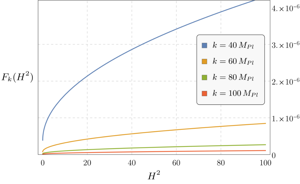
As one can observe from the figure, in $d=3$ there exist trajectories which depart from the NGFP in the UV and reach the GFP in the IR (magenta lines). These trajectories are separatrix lines which connect the two fixed points. In the present context only this type of trajectories is physical, since they give a positive and finite Newton coupling in the IR. All other trajectories (blue lines) correspond to Newton couplings which are either negative or divergent in the IR. The flow of $F_{k}(H^{2})$ of Eq. (4.12) takes a simple form. This function is non-analytic in $H^{2}$, and the couplings $f_{i}(k)$ exhibit canonical scaling for all values of the RG scale $k$. The evolution of $F_{k}$ is shown in Fig. 3 for $c_{0}=c_{1}=1$ and $d=3$, while the projection of the full RG flow of $F_{k}$ and $g_{k}$ on various two-dimensional theory sub-spaces is depicted in Fig. 4.

Let us finally remark that the solution in Eqs. (4.15) and (4.16) is unphysical, since its IR behavior is not analytic in the curvature invariants. However, due to the non-linearity of the flow equations for $g_{k}$ and $F_{k}$, the solution we found in this section might not be unique. Indeed, in the following we shall seek (analytic) solutions, first via an $\epsilon$-expansion about $d=1$ and then via polynomial truncations. Let us note that computations based on a truncated derivative expansion of $F_{k}$, i.e. on a Taylor expansion of the function $F_{k}$ about $H=0$, can only provide approximations to scaling solutions for $F_{k}$ which are both even and analytic in $H=0$. In other words, since the solution found in this section is non-analytic in $H^{2}$, it is not accessible by polynomial truncations.

In this section we investigate the flow equations via an $\epsilon$-expansion. To this end, for convenience we shall write all functions in terms of $x=H/k$. As we have discussed in the preceding section, the flow equation for $\mathcal{F}_{k}$ is considerably complicated. However, the flow equation for $g_{k}$ is simpler, and expressing the functional dependence on $H^{2}$ in terms of $x$ it reads

$\displaystyle k\partial_{k}{g}_{k}=(d-1)\,g_{k}-\frac{d+3+\mathcal{D}_{k}[\mathcal{F}_{k}]}{3\cdot 2^{d+1}\,\pi^{\frac{d}{2}+1}\,\Gamma(\frac{d}{2}+1)}\,g^{2}_{k}\,,$

(4.19)

where we have defined the functional

$\displaystyle\mathcal{D}_{k}[\mathcal{F}_{k}]\equiv\frac{k\partial_{k}\mathcal{F}_{k}^{\prime}}{\mathcal{F}_{k}^{\prime}}\bigg|_{x=0}$

(4.20)

for later convenience. Notice that here, and in the ensuing discussion, primes denote derivatives with respect to $x$.

Assuming that at a fixed point $\mathcal{D}_{k}[\mathcal{F}_{k}]$ is well-defined¹⁰¹⁰ 10 This assumption can be self-consistently checked, at least within an $\epsilon$-expansion or truncations., in general one finds two fixed points for $g_{k}$. Since for $\epsilon\equiv d-1\ll 1$ this fixed point is $\mathcal{O}(\epsilon)$, this motivates studying the RG flow within an $\epsilon$-expansion, where the flow equation for $\mathcal{F}_{k}$ dramatically simplifies.

While the solution that we have described in the preceding section is exact, its low-energy behavior is phenomenologically not viable. Hence, motivated by the fact that for $d=1$ the Newton coupling is classically marginal, in this section we investigate the RG flow of $\mathcal{F}_{k}$ and $g_{k}$ at leading order in an $\epsilon$-expansion, setting $d=1+\epsilon$.

In order to properly account for the scaling of each term in the flow equations as $\epsilon\to 0^{+}$, one must specify an ansatz for $g_{k}$ and $\mathcal{F}_{k}$. A consistent ansatz for $g_{k}$ is simply a function $g_{k}=\epsilon\,\gamma_{k}$, with $\gamma_{k}=\mathcal{O}(1)$, which flows from a positive fixed point $\gamma_{*}$ in the UV (if $\mathcal{D}_{k}$ is regular in the UV) to zero in the IR. A consistent ansatz for $\mathcal{F}_{k}$ is then

$\displaystyle\mathcal{F}_{k}(x)=\frac{v_{k}(x)}{\epsilon\,\gamma_{k}}+w_{k}(x)\,\,,$

(4.21)

with $v_{k}(x)\,,\,w_{k}(x)=\mathcal{O}(1)$. This ansatz is motivated by the fact that in the IR regime $\mathcal{F}_{k}$ is expected to adhere to the perturbative result, while the corrections are expected to be sub-leading in $\epsilon$.

Using the aforementioned ansatz for $g_{k}$ and $\mathcal{F}_{k}$, the flow equations simplify considerably and, assuming that $\mathcal{D}_{k}[\mathcal{F}_{k}]$ is non-singular¹¹¹¹ 11 We shall verify this assumption a posteriori., at leading order they take the form

	$\displaystyle$	$\displaystyle k\partial_{k}{\gamma}_{k}=\epsilon\,\frac{\gamma_{k}}{\gamma_{*}}\left(\gamma_{*}-\gamma_{k}-\frac{1}{4}\,\gamma_{k}\,\mathcal{D}_{k}[v_{k}]\right)\,,$		(4.22)
		$\displaystyle\frac{k\partial_{k}{v}_{k}-x\,v_{k}^{\prime}+2v_{k}}{\epsilon\,\gamma_{k}}=\mathcal{O}(1)\,,$

where $\gamma_{*}=\frac{3}{2}\,\pi^{2}$ is the fixed-point value of $\gamma_{k}$. Correspondingly, the (dimensionful) Newton coupling scales as

$\displaystyle G_{k}\sim\frac{3\pi}{32}\,\epsilon\,k^{-\epsilon}$

(4.23)

in the UV. The second line of Eq. (4.22) then implies that $v_{k}(x)=\frac{V(k\,x)}{k^{2}}$, where we require that the arbitrary function $V$ be analytic at the origin in order to be consistent with perturbative $\alpha^{\prime}$-corrections. Furthermore, in order to allow for a UV fixed point, the function $v_{k}(x)$ must be at most quadratic,

$\displaystyle v_{k}(x)=\frac{\Lambda}{k^{2}}+\frac{x^{2}}{\zeta_{*}}\,.$

(4.24)

Here the coefficient of $x^{2}$ is the marginal deformation corresponding to the wave-function renormalization of $\Phi$, as discussed in the preceding section. In addition, this solution has $\mathcal{D}_{k}[v_{k}]=0$, so that $\mathcal{D}_{k}[\mathcal{F}_{k}]=\mathcal{O}(\epsilon)$ upon including the sub-leading term $w_{k}(x)$. The flow equation for $\gamma_{k}$ can then be solved exactly. Its solution reads

$\displaystyle\gamma_{k}=\frac{\gamma_{*}}{1+c\,k^{-\epsilon}}\,,$

(4.25)

where $c$ is an integration constant. Interestingly, this solution matches the result in Eq. (4.15) that we have found in Section 4.2 for $d=1+\epsilon$. In particular, for $c>0$ the flow interpolates smoothly between $\gamma_{*}=\frac{3}{2}\,\pi^{2}$ in the UV and zero in the IR, where $\gamma_{k}$ scales as $\gamma_{k}\sim\frac{\gamma_{*}}{c}\,k^{\epsilon}$ and, correspondingly,

$\displaystyle G_{k}\sim\frac{3\pi}{32}\,\frac{\epsilon}{c}\,.$

(4.26)

Since $\gamma_{k}$ flows very slowly, with $\dot{\gamma_{k}}\sim\epsilon\,\gamma_{k}$, one can neglect contributions involving $\dot{\gamma_{k}}$ in the sub-leading flow equation for $w_{k}$, since the latter involves also $\mathcal{O}(1)$ terms which dominate over those proportional to $k\partial_{k}\gamma_{k}$. Using these results and observations, the resulting flow equation for $w_{k}$ can be solved analytically, yielding

	$\displaystyle\gamma_{*}\,w_{k}(x)$	$\displaystyle=\frac{1}{2}+\left(\frac{3}{4}-\frac{\gamma_{*}}{\gamma_{k}}\right)\frac{\Lambda}{k^{2}}\,\log\left(\frac{k}{k_{0}}\right)+\frac{3\Lambda}{8k^{2}}\,\log\left(4-\frac{2\Lambda}{k^{2}}-\frac{x^{2}}{\zeta_{*}}\right)$		(4.27)
		$\displaystyle+\left(\left(\frac{\gamma_{*}}{\gamma}-\frac{1}{2}\right)\log\left(x\right)+\frac{1}{4}\,\log\left(4-\frac{2\Lambda}{k^{2}}-\frac{x^{2}}{\zeta_{*}}\right)\right)\frac{x^{2}}{\zeta_{*}}$
		$\displaystyle+\left(1+\frac{\Lambda}{4k^{2}}+\frac{x^{2}}{4\zeta_{*}}\right)\frac{\text{arctanh}\left(B_{k}(x)\right)}{B_{k}(x)}$
		$\displaystyle+\gamma_{*}\,\frac{W(k\,x)}{k^{2}}\,,$

where we have defined the combination

$\displaystyle B_{k}(x)\equiv\frac{x}{\sqrt{\zeta_{*}}\sqrt{\frac{2\Lambda}{k^{2}}-4+\frac{2x^{2}}{\zeta_{*}}}}$

(4.28)

and, once more, $W$ is an arbitrary function which we choose according to

$\displaystyle\frac{W(k\,x)}{k^{2}}=\frac{w_{0}}{k^{2}}+w_{2}\,x^{2}\,,$

(4.29)

with $w_{0}\,,w_{2}$ constants. The arbitrary scale $k_{0}$ can thus be shifted modifying $w_{0}$, while $w_{2}$ can be fixed by requiring that the quadratic terms reproduce the classical contribution $\frac{d\,x^{2}}{\zeta_{*}\,g_{k}}$ in the IR.

The large-$x$ behavior of the resulting solution $\mathcal{F}_{k}=\frac{v_{k}}{\epsilon\,\gamma_{k}}+w_{k}$ is consistent on dimensional grounds: it corresponds, at fixed $\dot{\sigma}=k\,x$, to the small-$k$ regime, which is perturbative and ought to reconstruct the classically marginal operator $\propto x^{2+\epsilon}\propto R^{\frac{D}{2}}$. Indeed,

$\displaystyle\mathcal{F}_{k}(x)\sim\frac{x^{2}}{\zeta_{*}\,g_{k}}\left(1+\epsilon\,\log\left(x\right)\right)\sim\frac{x^{2+\epsilon}}{\zeta_{*}\,g_{k}}\,.$

(4.30)

Using these results, one can derive the leading-order IR coefficients for higher-derivative corrections to the classical Lagrangian, which have the correct classical scaling. As a result, the dependence on $k$ disappears once the dimensionless variable $x$ is replaced by $x=\frac{H}{k}$. In detail, expanding $\mathcal{F}_{k}(x)$ in powers of $\frac{x}{\sqrt{\zeta_{*}}}$ and setting $\zeta_{*}=1$, the first few corrections to the classical Lagrangian read

$\displaystyle e^{\Phi}\,\mathcal{L}_{\text{HD}}\sim\frac{29}{480\pi^{2}\Lambda}\,H^{4}-\frac{53}{3360\pi^{2}\Lambda^{2}}\,H^{6}+\frac{1591}{241920\pi^{2}\Lambda^{3}}\,H^{8}\,.$

(4.31)

These corrections are $\mathcal{O}(\epsilon)$ with respect to the “classical” terms, whose leading-order IR contribution to the Lagrangian takes the form

$\displaystyle e^{\Phi}\,\mathcal{L}_{\text{tree}}\sim\frac{1}{16\pi G_{\text{N}}}\left(-\dot{\Phi}^{2}+\Lambda+H^{2}\right)$

(4.32)

at a suitable IR scale $k=k_{\text{IR}}$ such that $g_{k_{\text{IR}}}=16\pi G_{\text{N}}+\mathcal{O}(\epsilon)$. This identifies the relevant deformation $\Lambda$ as the leading contribution to the low-energy cosmological constant in the string-frame¹²¹² 12 In the Einstein frame, it takes the form of an exponential potential for the dilaton $V(\phi)=\Lambda\,e^{\frac{4}{D-2}\,\phi}$.. The size of the quartic correction approaches that of the classical curvature term when

$\displaystyle H^{2}\approx\Lambda\,,$

(4.33)

from which one could be tempted to identify $\Lambda\approx\frac{1}{\alpha^{\prime}}$ as an UV cutoff scale. Indeed, the precise value of $\Lambda$ is proportional to $\frac{D_{\text{crit}}-D}{\alpha^{\prime}}$, and encodes the deviation from the critical dimension Veneziano:1991ek; Fradkin:1984pq; Callan:1985ia. The coefficients in Eq. (4.31) can also be obtained by expanding the leading-order (in $\epsilon$) IR result

$\displaystyle e^{\Phi}\,\mathcal{L}_{\text{HD}}\sim\frac{\Lambda}{6\pi^{2}}\,L\left(\frac{H^{2}}{\Lambda}\right)$

(4.34)

in powers of $H$, where

	$\displaystyle L(s)$	$\displaystyle\equiv-1-\frac{23}{12}\,s+\left(\frac{3}{2}+s\right)\log\left(1+\frac{s}{2}\right)$		(4.35)
		$\displaystyle+\left(1+s\right)^{\frac{3}{2}}\,\sqrt{\frac{2}{s}}\,\text{arctanh}\left(\sqrt{\frac{s}{2\left(1+s\right)}}\right)\,.$

All in all, reinstating the lapse $n$, the leading-order (in $\epsilon$) IR string-frame effective action for cosmological ansatze reads

$\displaystyle\Gamma_{\text{string}}=\frac{\text{Vol}_{1+\epsilon}}{16\pi G_{\text{N}}}\int dt\,n\,e^{-\Phi}\left[\Lambda-\frac{\dot{\Phi}^{2}}{n^{2}}+\frac{\dot{\sigma}^{2}}{n^{2}}+\frac{8}{3\pi}\,G_{\text{N}}\,\Lambda\,L\left(\frac{\dot{\sigma}^{2}}{n^{2}\,\Lambda}\right)\right]\,.$

(4.36)

In Section 4.6 we shall comment on some potential cosmological consequences of these results, assuming that similar solutions and effective actions extend to the phenomenologically relevant case of $D=4$ spacetime dimensions.

The flow equations for $g_{k}$ and $F_{k}$ admit an exact non-analytic solution valid for any dimension $D$ (cf. Section 4.2) and an analytic solution in $D=(2+\epsilon)$ dimensions, characterized by an UV fixed point with $g_{\ast}>0$ and a phenomenologically viable IR limit (cf. Section 4.3). If the latter solution extended to $D=4$, the theory would be characterized by a UV fixed point with $g_{\ast}>0$ and a positive cosmological constant in the IR, thus realizing a scenario similar to the one proposed in deAlwis:2019aud. In this section we investigate whether the analytic solution found in $D=(2+\epsilon)$ dimensions can indeed extend to $D=4$.

Since an analytic exact solution in arbitrary dimensions $d$ cannot be found in closed form, in order to investigate the extension of the fixed point found in the previous section to $d=3$ we shall truncate the theory space choosing an ansatz for $F_{k}$ of the form¹³¹³ 13 The condition that $F_{k}$ be even in $H$ simplifies the computation of beta functions, and is required by T-duality.

$$F_{k}(H^{2})=\sum_{n=1}^{N}f_{2n-2}(k)\left(k^{-2}H\right)^{2n-2},$$

(4.37)

with $N$ finite. For a given truncation order $N$, one can determine the beta functions for all couplings associated with (even) powers of $H$ up to the order $H^{2(N-1)}$. Specifically, once $N$ is chosen, the ansatz for $F_{k}$ is to be replaced into Eq. (4.7). The beta functions $\beta_{n}\equiv k\partial_{k}f_{n}(k)$ for the couplings $\{f_{0}(k),\dots,f_{2N-2}(k)\}$ can then be computed expanding the flow equation for $F_{k}$ about $H=0$ up to order $N$ and requiring that the coefficients of the expansion vanish. For a given $N$, one can thus investigate the fixed-point structure of the flow equations as a function of $d$. One can then investigate the robustness of the results progressively enlarging the truncation order $N$. In fact, if a fixed-point functional exists in the full theory space and is analytic, it should be possible to detect it within truncations, and its critical exponents should converge to stable values upon increasing the truncation order. Vice versa, if a fixed point disappears increasing the truncation order, or if its critical exponents do not converge, it is likely that the fixed point is spurious, i.e., that it is a truncation artifact rather than a genuine feature of the theory. In the following we shall apply these techniques, investigating the fixed-point structure of the truncated flow of $F_{k}$ up to $N=5$, namely up to $\mathcal{O}(H^{10})$.

For any dimension $D$ there is a line of GFPs. The universality properties of this free fixed point are summarized in Tab. 1 and Tab. 2 for $D=2$ and $D=4$ respectively.

References

- (1) S. Weinberg, Critical Phenomena for Field Theorists, Erice Subnuclear Physics (1976) .
- (2) C. Wetterich, Exact evolution equation for the effective potential, Physics Letters B 301 (1993) 90.
- (3) J. Berges, N. Tetradis and C. Wetterich, Non-perturbative renormalization flow in quantum field theory and statistical physics, Physics Reports 363 (2002) 223 [hep-ph/0005122].
- (4) N. Dupuis, L. Canet, A. Eichhorn, W. Metzner, J. Pawlowski, M. Tissier et al., The nonperturbative functional renormalization group and its applications, 2006.04853.
- (5) I. Balog, H. Chaté, B. Delamotte, M. Marohnic and N. Wschebor, Convergence of Nonperturbative Approximations to the Renormalization Group, Phys. Rev. Lett. 123 (2019) 240604 [1907.01829].
- (6) A. Platania and C. Wetterich, Non-perturbative unitarity and fictitious ghosts in quantum gravity, Phys. Lett. B 811 (2020) 135911 [2009.06637].
- (7) R. Percacci, An Introduction to Covariant Quantum Gravity and Asymptotic Safety, vol. 3 of 100 Years of General Relativity. World Scientific, 2017, 10.1142/10369.
- (8) M. Reuter and F. Saueressig, Quantum Gravity and the Functional Renormalization Group. Cambridge University Press, 2019.
- (9) A. Eichhorn and T. Koslowski, Flowing to the continuum in discrete tensor models for quantum gravity, Ann. Inst. H. Poincare Comb. Phys. Interact. 5 (2018) 173 [1701.03029].
- (10) A. Eichhorn, J. Lumma, A. D. Pereira and A. Sikandar, Universal critical behavior in tensor models for four-dimensional quantum gravity, JHEP 02 (2020) 110 [1912.05314].
- (11) J. Ambjorn, A. Goerlich, J. Jurkiewicz and R. Loll, Nonperturbative Quantum Gravity, Phys. Rept. 519 (2012) 127 [1203.3591].
- (12) J. Laiho, S. Bassler, D. Du, J. Neelakanta and D. Coumbe, Recent results in Euclidean dynamical triangulations, Acta Phys. Polon. Supp. 10 (2017) 317 [1701.06829].
- (13) R. Loll, Quantum Gravity from Causal Dynamical Triangulations: A Review, Class. Quant. Grav. 37 (2020) 013002 [1905.08669].
- (14) J. Ambjorn, S. Jordan, J. Jurkiewicz and R. Loll, A Second-order phase transition in CDT, Phys. Rev. Lett. 107 (2011) 211303 [1108.3932].
- (15) J. Laiho and D. Coumbe, Evidence for Asymptotic Safety from Lattice Quantum Gravity, Physical Review Letters 107 (2011) 161301 [1104.5505].
- (16) J. Laiho, S. Bassler, D. Coumbe, D. Du and J. T. Neelakanta, Lattice Quantum Gravity and Asymptotic Safety, ArXiv e-prints (2016) [1604.02745].
- (17) J. Ambjorn, D. N. Coumbe, J. Gizbert-Studnicki and J. Jurkiewicz, Searching for a continuum limit in causal dynamical triangulation quantum gravity, Physical Review D 93 (2016) 104032 [1603.02076].
- (18) A. Platania and F. Saueressig, Functional Renormalization Group Flows on Friedman–Lemaître–Robertson–Walker backgrounds, Found. Phys. 48 (2018) 1291 [1710.01972].
- (19) B. Knorr and F. Saueressig, Towards reconstructing the quantum effective action of gravity, Phys. Rev. Lett. 121 (2018) 161304 [1804.03846].
- (20) J. Ambjørn, J. Gizbert-Studnicki, A. Görlich, J. Jurkiewicz and D. Németh, The phase structure of Causal Dynamical Triangulations with toroidal spatial topology, JHEP 06 (2018) 111 [1802.10434].
- (21) E. Fradkin and A. A. Tseytlin, Effective Action Approach to Superstring Theory, Phys. Lett. B 160 (1985) 69.
- (22) J. Callan, Curtis G., E. Martinec, M. Perry and D. Friedan, Strings in Background Fields, Nucl. Phys. B 262 (1985) 593.
- (23) J. Callan, Curtis G., I. R. Klebanov and M. Perry, String Theory Effective Actions, Nucl. Phys. B 278 (1986) 78.
- (24) A. M. Polyakov, Quantum Geometry of Bosonic Strings, Phys. Lett. B 103 (1981) 207.
- (25) A. M. Polyakov, Quantum Geometry of Fermionic Strings, Phys. Lett. B 103 (1981) 211.
- (26) D. Amati and C. Klimcik, Strings in a Shock Wave Background and Generation of Curved Geometry from Flat Space String Theory, Phys. Lett. B 210 (1988) 92.
- (27) D. Amati and C. Klimcik, Nonperturbative Computation of the Weyl Anomaly for a Class of Nontrivial Backgrounds, Phys. Lett. B 219 (1989) 443.
- (28) K. Meissner and G. Veneziano, Symmetries of cosmological superstring vacua, Phys. Lett. B 267 (1991) 33.
- (29) K. A. Meissner, Symmetries of higher order string gravity actions, Phys. Lett. B 392 (1997) 298 [hep-th/9610131].
- (30) O. Hohm and B. Zwiebach, T-duality Constraints on Higher Derivatives Revisited, JHEP 04 (2016) 101 [1510.00005].
- (31) O. Hohm and B. Zwiebach, Non-perturbative de Sitter vacua via corrections, Int. J. Mod. Phys. D 28 (2019) 1943002 [1905.06583].
- (32) O. Hohm and B. Zwiebach, Duality invariant cosmology to all orders in ’, Phys. Rev. D 100 (2019) 126011 [1905.06963].
- (33) P. Wang, H. Wu, H. Yang and S. Ying, Construct corrected or loop corrected solutions without curvature singularities, JHEP 01 (2020) 164 [1910.05808].
- (34) H. Bernardo, R. Brandenberger and G. Franzmann, O covariant string cosmology to all orders in , JHEP 02 (2020) 178 [1911.00088].
- (35) H. Bernardo and G. Franzmann, -Cosmology: solutions and stability analysis, JHEP 05 (2020) 073 [2002.09856].
- (36) C. A. Núñez and F. E. Rost, New non-perturbative de Sitter vacua in -complete cosmology, 2011.10091.
- (37) S. W. Hawking, QUANTUM COSMOLOGY, in Les Houches Summer School on Theoretical Physics: Relativity, Groups and Topology, pp. 333–379, 7, 1983.
- (38) S. W. Hawking, The Quantum State of the Universe, Adv. Ser. Astrophys. Cosmol. 3 (1987) 236.
- (39) A. Vilenkin, Approaches to quantum cosmology, Phys. Rev. D 50 (1994) 2581 [gr-qc/9403010].
- (40) A. Ashtekar and P. Singh, Loop Quantum Cosmology: A Status Report, Class. Quant. Grav. 28 (2011) 213001 [1108.0893].
- (41) M. Bojowald, Quantum cosmology: a review, Rept. Prog. Phys. 78 (2015) 023901 [1501.04899].
- (42) A. Bonanno and M. Reuter, Renormalization group improved black hole space-times, Phys. Rev. D62 (2000) 043008 [hep-th/0002196].
- (43) S. Weinberg, Ultraviolet divergences in quantum theories of gravitation., in General Relativity: An Einstein centenary survey, S. W. Hawking and W. Israel, eds., pp. 790–831, 1979.
- (44) R. Gastmans, R. Kallosh and C. Truffin, Quantum Gravity Near Two-Dimensions, Nucl. Phys. B 133 (1978) 417.
- (45) S. Christensen and M. Duff, Quantum Gravity in Two + Dimensions, Phys. Lett. B 79 (1978) 213.
- (46) H. Kawai and M. Ninomiya, Renormalization Group and Quantum Gravity, Nucl. Phys. B 336 (1990) 115.
- (47) H. Kawai, Y. Kitazawa and M. Ninomiya, Scaling exponents in quantum gravity near two-dimensions, Nucl. Phys. B 393 (1993) 280 [hep-th/9206081].
- (48) H. Kawai, Y. Kitazawa and M. Ninomiya, Ultraviolet stable fixed point and scaling relations in (2+epsilon)-dimensional quantum gravity, Nucl. Phys. B 404 (1993) 684 [hep-th/9303123].
- (49) H. Kawai, Y. Kitazawa and M. Ninomiya, Renormalizability of quantum gravity near two-dimensions, Nucl. Phys. B 467 (1996) 313 [hep-th/9511217].
- (50) T. Aida and Y. Kitazawa, Two loop prediction for scaling exponents in (2+epsilon)-dimensional quantum gravity, Nucl. Phys. B 491 (1997) 427 [hep-th/9609077].
- (51) G. Obied, H. Ooguri, L. Spodyneiko and C. Vafa, De Sitter Space and the Swampland, 1806.08362.
- (52) H. Ooguri, E. Palti, G. Shiu and C. Vafa, Distance and de Sitter Conjectures on the Swampland, Phys. Lett. B 788 (2019) 180 [1810.05506].
- (53) S. K. Garg and C. Krishnan, Bounds on Slow Roll and the de Sitter Swampland, JHEP 11 (2019) 075 [1807.05193].
- (54) E. Palti, The Swampland: Introduction and Review, Fortsch. Phys. 67 (2019) 1900037 [1903.06239].
- (55) J. Mourad and A. Sagnotti, Vacua from Dilaton Tadpoles and Form Fluxes, Phys. Lett. B768 (2017) 92 [1612.08566].
- (56) A. Maloney, E. Silverstein and A. Strominger, De Sitter space in noncritical string theory, in Workshop on Conference on the Future of Theoretical Physics and Cosmology in Honor of Steven Hawking’s 60th Birthday, pp. 570–591, 5, 2002, hep-th/0205316.
- (57) D. Friedan, E. J. Martinec and S. H. Shenker, Conformal Invariance, Supersymmetry and String Theory, Nucl. Phys. B 271 (1986) 93.
- (58) T. Buscher, A Symmetry of the String Background Field Equations, Phys. Lett. B 194 (1987) 59.
- (59) T. Buscher, Path Integral Derivation of Quantum Duality in Nonlinear Sigma Models, Phys. Lett. B 201 (1988) 466.
- (60) A. A. Tseytlin, Duality Symmetric Formulation of String World Sheet Dynamics, Phys. Lett. B 242 (1990) 163.
- (61) D. S. Berman, N. B. Copland and D. C. Thompson, Background Field Equations for the Duality Symmetric String, Nucl. Phys. B 791 (2008) 175 [0708.2267].
- (62) C. Hull and B. Zwiebach, Double Field Theory, JHEP 09 (2009) 099 [0904.4664].
- (63) O. Hohm, C. Hull and B. Zwiebach, Generalized metric formulation of double field theory, JHEP 08 (2010) 008 [1006.4823].
- (64) N. B. Copland, A Double Sigma Model for Double Field Theory, JHEP 04 (2012) 044 [1111.1828].
- (65) S. Groot Nibbelink and P. Patalong, A Lorentz invariant doubled world-sheet theory, Phys. Rev. D 87 (2013) 041902 [1207.6110].
- (66) G. Aldazabal, D. Marques and C. Nunez, Double Field Theory: A Pedagogical Review, Class. Quant. Grav. 30 (2013) 163001 [1305.1907].
- (67) S. Hronek and L. Wulff, O(D,D) and the string expansion: An obstruction, 2012.13410.
- (68) T. Codina, O. Hohm and D. Marques, A Puzzle Concerning String Dualities at Order , arXiv e-prints (2020) arXiv:2012.15677 [2012.15677].
- (69) F. Hassler and T. B. Rochais, O(,)-covariant two-loop -functions and Poisson-Lie T-duality, 2011.15130.
- (70) G. Veneziano, Scale factor duality for classical and quantum strings, Phys. Lett. B 265 (1991) 287.
- (71) C. Krishnan, de Sitter, -Corrections \& Duality Invariant Cosmology, JCAP 10 (2019) 009 [1906.09257].
- (72) T. R. Morris, The Exact Renormalization Group and Approximate Solutions, International Journal of Modern Physics A 9 (1994) 2411 [hep-ph/9308265].
- (73) M. Reuter, Nonperturbative evolution equation for quantum gravity, Phys. Rev. D57 (1998) 971 [hep-th/9605030].
- (74) D. F. Litim, Optimized renormalization group flows, Phys. Rev. D 64 (2001) 105007 [hep-th/0103195].
- (75) E. S. Fradkin and A. A. Tseytlin, Effective Field Theory from Quantized Strings, Phys. Lett. B 158 (1985) 316.
- (76) S. de Alwis, A. Eichhorn, A. Held, J. M. Pawlowski, M. Schiffer and F. Versteegen, Asymptotic safety, string theory and the weak gravity conjecture, Phys. Lett. B 798 (2019) 134991 [1907.07894].
- (77) I. Basile and A. Platania, String Tension between de Sitter vacua and Curvature Corrections, 2103.06276.