The cost of universality: A comparative study of the overhead
of state distillation and code switching with color codes
Abstract
Estimating and reducing the overhead of fault tolerance (FT) schemes is a crucial step toward realizing scalable quantum computers. Of particular interest are schemes based on two-dimensional (2D) topological codes such as the surface and color codes which have high thresholds but lack a natural implementation of a non-Clifford gate. In this work, we directly compare two leading FT implementations of the gate in 2D color codes under circuit noise across a wide range of parameters in regimes of practical interest. We report that implementing the gate via code switching to a 3D color code does not offer substantial savings over state distillation in terms of either space or space-time overhead. We find a circuit noise threshold of for the gate via code switching, almost an order of magnitude below that achievable by state distillation in the same setting. To arrive at these results, we provide and simulate an optimized code switching procedure, and bound the effect of various conceivable improvements. Many intermediate results in our analysis may be of independent interest. For example, we optimize the 2D color code for circuit noise yielding its largest threshold to date , and adapt and optimize the restriction decoder finding a threshold of for the 3D color code with perfect measurements under noise. Our work provides a much-needed direct comparison of the overhead of state distillation and code switching, and sheds light on the choice of future FT schemes and hardware designs.
I Introduction
In this section we first provide this work’s motivation and a summary of our main results in Section I.1, and then review some relatively standard but important background material that we will refer to throughout the paper. In Section I.2 we describe the noise models and simulation approaches that we use to analyze and simulate state distillation and code switching. In Section I.3 we provide some basic information about the color codes. In Section I.4 we review how to implement logical operations using 2D color codes. Finally in Section I.4 we review state distillation.
I.1 Motivation and summary of results
Recent progress in demonstrating operational quantum devices Nigg et al. 2014; Barends et al. 2014; Córcoles et al. 2013; Ofek et al. 2016; Arute et al. 2019 has brought the noisy intermediate-scale quantum era Preskill 2018, where low-depth algorithms are run on small numbers of qubits. However, to handle the cumulative effects of noise and faults as these quantum systems are scaled, fault-tolerant (FT) schemes Shor 1996; Knill 2005; Steane 1997; Aharonov and Ben-Or 1997; Preskill 1998; Aliferis et al. 2005; Raussendorf and Harrington 2007; Raussendorf et al. 2007; Dennis et al. 2002 will be needed to reliably implement universal quantum computation. FT schemes encode logical information into many physical qubits and implement logical operations on the encoded information, all while continually diagnosing and repairing faults. This requires additional resources, and much of the current research in quantum error correction (QEC) is dedicated toward developing FT schemes with low overhead.
The choice of FT scheme to realize universal quantum computing has important ramifications. Good schemes can significantly enhance the functionality and lifetime of a given quantum computer. Moreover, FT schemes vary in their sensitivity to the hardware architecture and design, such as qubit quality Cross et al. 2009, connectivity, and operation speed. The understanding and choice of FT scheme will therefore influence the system design, from hardware to software, and developing an early understanding of the trade-offs is critical in our path to a scalable quantum computer.
At the base of most FT schemes is a QEC code which (given the capabilities and limitations of a particular hardware platform) should: (i) tolerate realistic noise (ii) have an efficient classical decoding algorithm to correct faults, and (iii) admit a FT universal gate set. In the search of good FT schemes we focus our attention on QEC codes which are known to achieve as many of these points as possible with low overhead. Topological codes are particularly compelling as they typically exhibit high accuracy thresholds with QEC protocols involving geometrically local quantum operations and efficient decoders; see e.g. Refs. Dennis et al. 2002; Brown et al. 2016; Duclos-Cianci and Poulin 2010; Anwar et al. 2014; Duclos-Cianci and Poulin 2013; Bravyi and Haah 2013; Duivenvoorden et al. 2019; Kubica and Preskill 2019; Vasmer et al. 2020; Bravyi et al. 2014; Darmawan and Poulin 2018; Nickerson and Brown 2019; Maskara et al. 2019; Chamberland and Ronagh 2018; Delfosse 2014; Kubica and Delfosse 2019. Two-dimensional (2D) topological codes such as the toric code Kitaev 1997; Bravyi and Kitaev 1998 and the color code Bombin and Martin-Delgado 2006 are particularly appealing for superconducting Fowler et al. 2012; Chamberland et al. 2020a; Chamberland et al. 2020b and Majorana Karzig et al. 2017; Chao et al. 2020 hardware, where qubits are laid out on a plane and quantum operations are limited to those involving neighboring qubits.
The FT implementation of logical gates with 2D topological codes poses some challenges. The simplest FT logical gates are applied transversally, i.e., by independently addressing individual physical qubits. These gates are automatically FT since they do not grow the support of errors. Unfortunately a QEC code which admits a universal set of transversal logical gates is ruled out by the Eastin-Knill theorem Eastin and Knill 2009; Zeng et al. 2011; Jochym-O’Connor et al. 2018. Furthermore, in 2D topological codes such gates can only perform Clifford operations Bravyi and König 2013; Pastawski and Yoshida 2014; Beverland et al. 2016; Webster et al. 2020. There are, however, many innovative approaches to achieve universality, which typically focus on implementing non-Clifford logical gates Bombin and Martin-Delgado 2007; Kubica et al. 2015; Vasmer and Browne 2019, which achieve universality when combined with the Clifford gates.
The standard approach to achieve universality with 2D topological codes is known as state distillation Bravyi and Kitaev 2005; Knill 2004a; Knill 2004b. It relies on first producing many noisy encoded copies of a state , also known as a magic state, and then processing them using Clifford operations to output a high fidelity encoded version of the state. The high-fidelity state can then be used to implement the non-Clifford gate. Despite significant recent improvements, the overhead of state distillation is expected to be large in practice Fowler et al. 2012; Litinski 2019. A compelling alternative is code switching via gauge fixing Paetznick and Reichardt 2013; Anderson et al. 2014; Bombin 2015a; Bombín 2016 to a 3D topological code which has a transversal gate. The experimental difficulty of moving to 3D architectures could potentially be justified if it significantly reduces the overhead compared to state distillation. To compare these two approaches and find which is most practical for consideration in a hardware design, a detailed study is required.
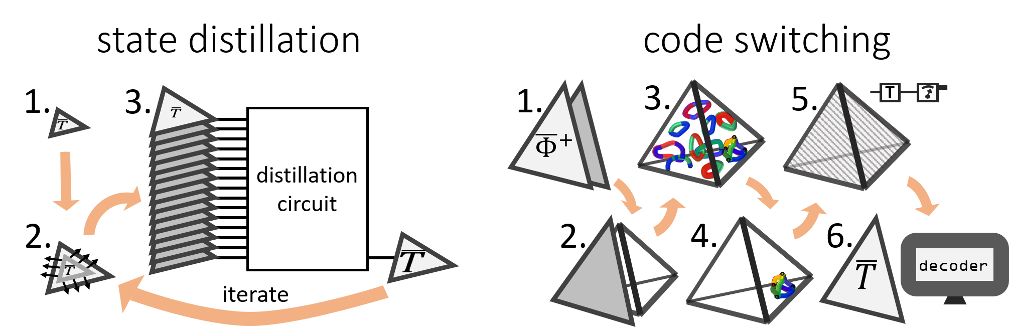
In our work, we estimate the resources needed to prepare high-fidelity states encoded in the 2D color code, via either state distillation or code switching. We assume that both approaches are implemented using quantum-local operations Bombin 2015b in 3D, i.e., quantum operations are noisy and geometrically local, whereas classical operations can be performed globally and perfectly (although they must be computationally efficient). In particular, we simulate these two approaches by implementing them with noisy circuits built from single-qubit state preparations, unitaries and measurements, and two-qubit unitaries between nearby qubits. For state distillation, this 3D setting allows a stack of 2D color code patches, whereas for code switching it allows to implement the 3D color code; see Fig. 1. We then seek to answer the following question: to prepare states of a given fidelity, are fewer resources required for state distillation or code switching?
Our main finding is that code switching does not offer substantial savings over state distillation in terms of both space overhead, i.e., the number of physical qubits required, and space time overhead, i.e., the space overhead multiplied by the number of physical time units required; see Fig. 2. State distillation significantly outperforms code switching over most of the circuit noise error rates and target state infidelities , except for the smallest values of , where code switching slightly outperformed state distillation. In our analysis we carefully optimize each step of code switching, and also investigate the effects of replacing each step by an optimal version to account for potential improvements. On the other hand we consider only a standard state distillation scheme, and using more optimized schemes such as Bravyi and Haah 2012; Haah et al. 2017a; Haah and Hastings 2018 would give further advantage to a state distillation approach. We also find asymptotic expressions which support our finding that state distillation requires lower overhead than code switching for and . In particular, the space and space-time overhead scale as and respectively, where for code switching and for the distillation scheme we implement.
(a) (b) (c) (d) (e) (f)
To arrive at our main simulation results, we accomplish the intermediate goals below.
2D color code optimization and analysis.—In Section II, we first adapt the projection decoder Delfosse 2014 to the setting where the 2D color code has a boundary and syndrome extraction is imperfect, as well as optimize the stabilizer extraction circuits. We find a circuit noise threshold greater than , which is the highest to date for the 2D color code, narrowing the gap to that of the surface code. We also analyze the noise equilibration process during logical operations in the 2D color code and provide an effective logical noise model.
Noisy state distillation analysis.—Using the effective logical noise model, we carefully analyse the overhead of state distillation in Section III. We strengthen the bounds on failure and rejection rate by explicitly calculating the effect of faults at each location in the Clifford state distillation circuits rather than simply counting the total number of locations Brooks 2013; Jochym-O’Connor et al. 2013; Jones 2013a; Fowler et al. 2012; Litinski 2019. We remark that we stack 2D color codes in the third dimension to implement logical operations such as the CNOT in constant time, whereas strictly 2D approaches such as lattice surgery would require a time proportional to code distance. The circuit-noise threshold for this state distillation scheme with the 2D color code is equal to the error correction threshold of .
Further insights into 3D color codes.—In Section IV, we provide a surprisingly direct way to switch between the 2D color code and the 3D subsystem color code. Our method exploits a particular gauge-fixing of the 3D subsystem color code for which the code state admits a local tensor product structure in the bulk and can therefore be prepared in constant time. We also adapt the restriction decoder Kubica and Delfosse 2019 to the setting where the 3D color code has a boundary and optimize it, which results in a threshold of 0.80(5)% and a better performance for small system sizes.
End-to-end code switching simulation.—Section V is the culmination of our work, where building upon results from the previous sections we provide a simplified recipe for code switching, detailing each step and specifying important optimizations. In our simulation, we exploit the special structure of the 3D subsystem color code to develop a method of propagating noise through the gates in the system, despite the believed computational hardness of simulating general circuits with many qubits and gates. We numerically find the failure probability of implementing the gate with code switching as a function of the code distance and the circuit noise strength, which, in turn, allows us to estimate the gate threshold to be . We not only find numerical estimates of the overhead of the fully specified protocol, but also bound the minimal overhead of a code switching protocol with various conceivable improvements, such as using optimal measurement circuits, and optimal classical algorithms for decoding and gauge fixing of the 3D color code.
This work provides a much-needed comparative study of the overhead of state distillation and code switching, and enables a deeper understanding of these two approaches to FT universal quantum computation. More generally, careful end-to-end analyses with this level of detail will become increasingly important to identify the most resource-efficient FT schemes and, in turn, to influence the evolution of quantum hardware. Although our study focuses on color codes, we expect our main finding, i.e., that code switching does not significantly outperform state distillation, to hold for other topological codes such as the toric code as considered in Ref. Vasmer and Browne 2019. Furthermore, we believe that state distillation will not be outperformed by code switching exploiting either 2D subsystem codes Bravyi and Cross 2015; Jochym-O’Connor and Bartlett 2016; Jones et al. 2016 or emulation of a 3D system with a dynamical 2D system Bombin 2018a; Brown 2020; Scruby et al. 2020; Iverson and Kubica 2021 since these schemes are even more constrained than when 3D quantum-local operations are allowed. We remark that there are other known FT techniques for implementing a universal gate set Hill et al. 2013; Yoder et al. 2016; Jochym-O’Connor and Laflamme 2014; Aliferis et al. 2005; Chamberland and Cross 2019; Chamberland and Noh 2020a, however they are not immediately applicable to large-scale topological codes. Nevertheless, we are hopeful that there are still new and ingenious FT schemes to be discovered that could dramatically reduce the overhead and hardware requirements for scalable quantum computing.
I.2 Noise and simulation
The noise model we use throughout the paper is the depolarizing channel, which on single- and two-qubit density matrices and has the action
| (1) | |||||
| (2) |
where the parameter can be interpreted as an error probability. The depolarizing channel leaves a single-qubit state unaffected with probability and applies an error , , or , each with probability . Similarly, the depolarizing channel leaves a two-qubit state unaffected with probability and with probability applies a nontrivial Pauli error .
We consider three standard scenarios,
- 1.
Depolarizing noise.—Error correction is implemented with perfect measurements following a single time unit, during which single-qubit depolarizing noise of strength acts. This is often referred to in the literature as the code capacity setting.
- 2.
Phenomenological noise.—Error correction is implemented with perfect measurements following each time unit, during which single-qubit depolarizing noise of strength acts. However the measurement outcome bits are flipped with probability .
- 3.
Circuit noise.—Measurements are implemented with the aid of ancilla qubits and a sequence of one- and two-qubit operations; see Fig. 3(a). One- and two-qubit unitary operations experience depolarizing noise of strength . One-qubit preparations and measurements fail with probability by producing an orthogonal state or flipping the outcome; see Fig. 3(b).
(a) (b)
In circuit noise, we approximate every noisy gate, i.e., Pauli , and operators, the Hadamard gate , the phase gate , the controlled-not gate CNOT, and the idle gate , by an ideal gate followed by the depolarizing channel on qubits acted on by the gate see Fig. 3. Preparations of the state orthogonal to that intended occur with probability , and measurement outcome bits are flipped with probability . We assume that all the elementary operations take the same time, which we refer to as one time unit.
For each of the three noise models, we will use error rate and noise strength interchangeably to describe the single parameter .
We assume a special form of noise on states, which is justified as follows. Consider an arbitrary single-qubit state
| (3) |
written in the orthonormal basis . Now consider a ‘twirling operation’ consisting of randomly applying the Clifford , with probability . This single-qubit Clifford gate can be implemented instantaneously and perfectly by a frame update.11 1 Since we assume throughout that arbitrary one- and two-qubit physical operations are allowed, single-qubit Clifford physical operations can actually be done ‘offline’ by tracking the basis of each physical qubit, and modifying future operations to be applied to that qubit accordingly. They are therefore perfect and instantaneous, as they only involve classical processing. Moreover, we will later see that logical Clifford operations can be done offline in 2D color codes such that the logical noise on encoded states can also be twirled offline. The state is transformed as follows
| (4) |
We therefore assume that the noisy state is of the form , or equivalently that each state is afflicted by a error with probability . Due to this simplified form of the noise, we use infidelity, which is defined by , interchangeably with the noise rate and noise strength to refer to the single parameter when describing errors on states.
For the purpose of defining pseudo-thresholds later, we find it useful to define the physical error probability for a time as the probability that a single physical qubit will have a nontrivial operator applied to it over time units under this noise model. It can be calculated as follows
| (5) |
where and . For example , , etc. Note that .
To simulate noise, for Clifford circuits we track the net Pauli operator which has been applied to the system by noisy operations using the standard binary symplectic representation. When non-Clifford operations are involved, we use modified techniques which are explained throughout the text.
To estimate the statistical uncertainty of any quantity of interest we use the bootstrap technique, i.e., we repeat sampling from the existing data set to evaluate . In particular, for we (i) randomly choose data points from the data set , where , (ii) evaluate the quantity using the data set . We remark that the same data point can be chosen multiple times in step (i). We then estimate the quantity of interest to be
| (6) |
Note that when reporting estimated values, we will use a digit in parenthesis to indicate the standard deviation of the preceding digit. For example, we write in place of .
We will often consider the failure probability of various tasks using a distance code and noise strength . We use the following ansatz that characterizes the generic feature that decreases exponentially with for any below the threshold value , i.e.,
| (7) |
where and are functions of alone. In particular, is smaller than one for . This can be considered a generalization of the heuristic behavior of error correction failure rate in topological codes for error rate in the vicinity of their threshold Fowler et al. 2012; Fowler 2013; Landahl et al. 2011.
I.3 Basics of 2D and 3D color codes
Here we briefly review some important features of color codes, focusing on 2D and 3D. We also specify the lattices and some notation we use throughout the paper. For a more complete review of the topics covered in this subsection, see Refs. Kubica and Beverland 2015; Bombin 2015a; Kubica 2018.
Color codes are topological QEC codes which can be defined on any -dimensional lattice composed of -simplices with -colorable vertices, where . Recall that -simplices are vertices, edges, triangles and tetrahedra, respectively. Qubits are placed on -simplices of the lattice; - and -type gauge generators are on - and -simplices, and - and -type stabilizer generators are on - and -simplices, where and . We say an operator is on a -simplex when its support comprises all the -simplices containing that -simplex.
(a)
 (b)
(b)
In this paper, we focus on color codes on two particular (families of) lattices: a 2D triangular lattice with a triangular boundary , and a 3D bcc lattice with a tetrahedral boundary ; see Fig. 4. We will occasionally refer to as the triangular lattice and as the tetrahedral lattice. Most of the time we rely on context and drop the subscript, simply writing . Members of these lattice families are parameterized by the code distance of color codes defined on them. We typically work with the dual lattice , but occasionally make use of the primal lattice . We remark that the graph constructed from the vertices and edges of the primal lattice is bipartite Kubica and Beverland 2015; see Fig. 4(a).
Given a lattice , it is useful to define as the set of all -simplices in . We will abuse notation and write (or equivalently ) to denote that a -simplex belongs to an -simplex , where . It is also useful to construct the color-restricted lattice , where is a set of colors, by removing from all the simplices, whose vertices have colors not only in . For example, the restricted lattice is obtained by keeping all the vertices of color or , as well as all the edges connecting them. We refer to the edges in as edges; similarly for other colors. For any subset of edges and any vertex we define a restriction as the subset of edges of incident to . We separate vertices in into two types: boundary vertices (the three and four outermost vertices in Fig. 4(a) and (b), respectively), and all others which we call interior vertices. We call edges connecting two boundary vertices boundary edges (there are three and six boundary edges in Fig. 4(a) and (b), respectively), and call all other edges interior edges. More generally, we denote the sets of interior objects by , which is the set of all -simplices in containing at least one interior vertex
On the 2D lattice, we define the stabilizer 2D color code as follows. Qubits are on triangles, and both - and -stabilizer generators are on interior vertices . This code has one logical qubit and string-like logical operators. One can implement the full Clifford group transversally on the 2D color code.
On the 3D lattice, we can have either a stabilizer color code22 2 There is another stabilizer code with parameters but we work only with the version here. (with and ) or a subsystem color code (with ). In both cases, there is one logical qubit and the physical qubits are on tetrahedra. For the 3D subsystem color code, - and -stabilizer generators are on interior vertices , while - and -gauge generators are on interior edges . Recall that for subsystem codes, logical Pauli operators come in two flavors: bare logical operators which commute with the gauge generators, and dressed logical operators which commute with the stabilizer generators. In the 3D subsystem color code, bare and dressed logical operators are sheet- and string-like, respectively. One can implement the full Clifford group transversally on the 3D subsystem color code.
For the 3D stabilizer color code, - and -stabilizer generators are on interior vertices and interior edges respectively. The logical Pauli and operators are string- and sheet-like, respectively. Crucially, the gate is a transversal logical operator. To implement it, we split the qubits in into two groups, white tetrahedra and black tetrahedra, such that no two tetrahedra of the same color share a face. Applying to white qubits and to black qubits implements the logical gate. For notational convenience we write , determined by the color of the qubit.
Lastly, it is useful to introduce the notions of vector spaces associated with the constituents of the lattice and linear maps between them. We define to be a vector space over with the set of -simplices as its basis. Note that the elements of are binary vectors and we can identify them with the subsets of . For any we define a generalized boundary operator , which is an -linear map specified on the basis element as follows
| (8) |
We remark that the standard boundary operator is a special case of the generalized boundary operator above if we choose . These boundary maps are helpful in discussing error correction with the color code. In particular, since the color code is a CSS code, we can cast the decoding problem in terms of chain complexes, and treat and errors and correction independently Delfosse 2014; Kubica and Delfosse 2019. For the 2D color code, the boundary map allows us to find for any error configuration its point-like syndrome via , where is the support of either or error. For the 3D stabilizer color code, the syndromes of and errors correspond to loop-like and point-like objects and can be found as and , where denotes the support of and error, respectively. In Section IV.2 we discuss in detail the structure of the loop-like gauge measurement outcomes for the 3D subsystem color code.
I.4 Fault-tolerant computation with 2D color codes
Here we briefly review an approach to implement quantum computation with a 3D stack of the 2D color codes as in Fig. 5(a). Note that alternatively we could lay out the 2D color codes on a 2D plane and use lattice surgery Landahl and Ryan-Anderson 2014, although many of the elementary logical operations, e.g. CNOT gates, would be slower than for a stack.
(a)  (b)
(b)
Error correction and decoding.—On each patch of the 2D color code, QEC is continuously performed. We use the term QEC cycle to refer to a full cycle of stabilizer extraction circuits producing a syndrome , i.e., the set of measured stabilizer generators with outcome .
In a scenario in which measurements are performed perfectly, a perfect measurement decoder is used to infer a correction for any error given the input . The correction will return the system to the code space if applied. The perfect measurement decoder fails if and only if is a nontrivial logical operator.
In a scenario in which measurements are not perfect, we consider a sequence of QEC cycles , with error introduced during each cycle, and observed syndrome for each. For simplicity we assume that the first and last cycle have no additional error and that the syndrome is measured perfectly. Then a faulty measurement decoder is a decoder with takes the full history of syndromes and outputs a correction such that has trivial syndrome. The faulty measurement decoder fails if and only if is a nontrivial logical operator. We discuss decoders for the 2D color code in detail in Section II.
Logical operations.—The elementary logical operations for the 2D color codes are implemented as follows.
- •
State preparation.—To prepare the state each data qubit is prepared in , then QEC cycles are performed, and the -type syndrome outcomes at the first cycle are inferred ( cycles are needed to do so fault-tolerantly). A -type fixing operator with the syndrome is applied. The state is prepared analogously.
- •
Idle operation.—A single QEC cycle is performed.
- •
Single-qubit Clifford gates.—As the gates are transversal, these are done in software by Pauli frame updates so are instantaneous and perfect.
- •
CNOT gate.—This is implemented by the application of a transversal CNOT between adjacent patches in the the stack, and followed by QEC cycles; see Section II.4 for details.
- •
SWAP gate.—This is implemented by swapping the data qubits on adjacent patches, and followed by a single QEC cycle.
- •
Measurement.—The readout of single-qubit measurements in the and basis is implemented by measuring each data qubit in the and basis. The output bit string is then processed in two stages: (1) a perfect measurement decoder is run to correct the bit string such that it satisfies all stabilizers, and then (2) the outcome is read off from the parity of the corrected bit string restricted to the support of any representative of the logical operator.
The above list consists of Clifford operations, which are not by themselves universal for quantum computation. In addition, we consider the following non-Clifford gate.
- •
gate. It is implemented using gate teleportation of an encoded state as shown in Fig. 5(b). We will consider the production of the encoded state by both state distillation and code switching.
I.5 State distillation
Here we briefly review state distillation Bravyi and Kitaev 2005; Knill 2004a, in which Clifford operations are used with postselection to convert noisy resource states into fewer but crucially less noisy resource states. In our analysis of the overhead of state distillation in Section III, we consider only the standard 15-to-1 state distillation protocol. However, given the wide range of state distillation protocols that have been proposed in recent years, we take the opportunity to attempt to consolidate the concepts behind them here. In particular, we outline three classes of state distillation protocols, which to our knowledge include all known proposals up to small variations. We then go on to describe a family of protocols recently introduced by Haah and Hastings Haah and Hastings 2018, for which the 15-to-1 protocol that we consider is an special instance. In our discussion here we will assume Clifford operations are perfect, although we will relax that assumption in Section III.
(a) (b)
(c)
Let be an operator stabilizing a resource state , i.e., , and be a non-Clifford unitary transforming into some stabilizer state , i.e., . We will refer to and as the resource stabilizer and resource rotator, respectively, and throughout when we write that should be applied, it can be implemented using by gate teleportation as in Fig. 5(b). The three classes of state distillation protocols are then summarized as follows (and depicted Fig. 6).
- (a)
Code projector then resource rotator.—We use a code with a transversal logical gate . We prepare the (noisy) logical state by first encoding the logical stabilizer state and then implementing the transversal gate (using copies of the noisy resource state ). Unencoding and postselecting on the measurement outcomes of the stabilizers of the code gives a distilled resource state with infidelity reduced from to for code distance . See schemes in Landahl and Cesare 2013; Bravyi and Kitaev 2005; Bravyi and Haah 2012; Haah and Hastings 2018; Hastings and Haah 2018.
- (b)
Resource stabilizer then code projector.—We use a code with a transversal logical gate . We start with noisy resource states , which by definition satisfy , then measure the stabilizers of the code. If all measurement outcomes are , then the state has been prepared, which can then be further decoded to yield a distilled resource state with infidelity suppressed from to . Note that this approach seems less promising than the other two since the probability of successful postselection is less than one even for perfect resource states. See schemes in Bravyi and Kitaev 2005; Reichardt 2005.
- (c)
Code projector then resource stabilizer.—We use a code with a transversal logical gate and assume that is a Pauli operator.33 3 If the unitary is in the third level of the Clifford hierarchy, then is a Clifford operator, but by using this approach with a code which implements a non-Clifford transversal gate , state distillation for higher-order schemes should be possible. First, we encode a resource state with infidelity in the code, giving , and then measure the logical operator and postselect on the outcome. To measure we use a measurement gadget consisting of the following three steps. First, apply using noisy states, each with infidelity . Second, apply the Clifford gate control-, controlled by an ancilla state . Third, apply using another noisy states, each with infidelity . After this gadget, the stabilizers are checked, and if all are satisfied, then the encoded state is decoded and kept as a distilled resource state. The output has infidelity suppressed to , but the suppression with respect to can be boosted by, for example, repeating the measurement gadget. See schemes in Knill 2004a; Knill 2004b; Meier et al. 2013; Jones 2013b; Duclos-Cianci and Poulin 2015; Campbell and O’Gorman 2016; Haah et al. 2017b.
Historically, the first state distillation protocol was proposed by Knill Knill 2004a (type c), which takes 15 input states of infidelity to produce an output of infidelity , with acceptance probability . Shortly after, Bravyi and Kitaev Bravyi and Kitaev 2005 proposed two schemes, the first of which is type a in our classification, but which has the same parameters as Knill’s (later the two schemes were shown to be mathematically equivalent Haah 2018). The second scheme in Ref. Bravyi and Kitaev 2005 is of type b and has less favorable parameters than the 15-to-1 scheme, but a higher state distillation threshold. Another type b scheme was found by Reichardt Reichardt 2005, which could successfully distill states arbitrarily close to the stabilizer polytope. In Ref. Bravyi and Haah 2012, type a schemes outputting multiple resource states were proposed. Multiple outputs were also achieved for type b schemes in Refs. Jones 2013b; Haah et al. 2017b. These ‘high rate ’ schemes have promising parameters and may perform well in certain regimes. However, they also tend to have large Clifford circuits likely inhibiting their practicality when including the effect of realistically noisy Clifford operations. Recently, Haah and Hastings introduced yet another family of state distillation protocols of type a Haah and Hastings 2018. These are based on puncturing quantum Reed-Muller codes and have both interesting asymptotic properties Hastings and Haah 2018 and appear to be practically favorable Haah and Hastings 2018. We review this family here, which includes the 15-to-1 scheme that we analyze in detail in Section III.
Haah-Hastings state distillation protocols.—This family of state distillation protocols Haah and Hastings 2018 involves first producing what we will call a Reed-Muller state on qubits, where , with a Clifford circuit of depth using CNOTs; see Fig. 7. This state has the property that for any subset of qubits, the state can be decomposed as a set of Bell pairs between those ‘punctured’ qubits and those which remain, namely
| (9) |
where the states of the punctured qubits have no bar, and where are logical basis states for a CSS code which is triply-even and that transversal implements a logical on each logical qubit of the code. Let the -distance be the weight of the smallest nontrivial -type logical operator of this code. To specify the CSS code, which we call the punctured Reed-Muller code, one can start with the - and -type stabilizer generators of the state (which, for example, could be specified by propagating the initial single-qubit stabilizers through the CNOT circuit in Fig. 7). Choosing a stabilizer generator set for in such a way that only one - and one -type generator have nontrivial support on each punctured qubit, these form logical operators and the remaining generators with no support on any punctured qubits form the stabilizer generators of the punctured Reed-Muller code.
The next step of the protocol is to apply a (noisy) gate to each non-punctured qubit,
| (10) |
To see this, note that . Finally, one measures the logical operators of the CSS code. If the measurement outcome of is +1, then the th punctured qubit is left in the state ; otherwise, the th punctured qubit is in the state , requiring a simple Pauli fix. In practice this is achieved by measuring all non-punctured qubits in the -basis, and post-processing. Note that post-processing the measurement outcomes also tells us what the -stabilizer generators for the CSS code are, which should all be in the absence of error. This, in turn provides, a postselection condition of the protocol. The scheme takes encoded states of infidelity , and outputs encoded states of infidelity , where is the number of nontrivial -type logical operators of minimal weight .
In Fig. 7 we show an instance of the Haah-Hastings protocol for , which we analyze more explicitly in Section II. To our knowledge, this instance was first shown in Ref. Fowler et al. 2012, and is essentially a modification of the 15-to-1 Bravyi-Kitaev protocol, which avoids the need of the unencoding part of the circuit in Fig. 6(a). Some larger instances of this family have very good properties for state distillation, although we do not analyze them in detail here.
II 2D color code analysis
In this section, we describe an efficient and optimized implementation of the 2D color code under circuit noise. First, in Section II.1 we adapt Delfosse’s color code projection decoder Delfosse 2014 to allow for boundaries in the lattice. Then, we further adapt the decoder to accommodate faulty measurements in Section II.2. We optimize the stabilizer extraction circuits in Section II.3, finding a circuit noise threshold of 0.37(1)%. This represents a significant improvement over the previous highest threshold value for the color code of 0.2% in Chamberland et al. 2020b, and brings it closer to the toric code threshold of near one percent44 4 In Ref. Wang et al. 2011, a threshold above was reported, however follow-up work Chamberland et al. 2020b failed to reproduce this result and reported .. However, we stress that we are primarily interested in the finite-size rather than asymptotic performance, and therefore take care to accurately account for effects that are often ignored when focusing on threshold alone, such as residual error. We believe the performance improvements we see over previous studies of the color code under circuit noise are due to our use of the hexagonal rather than the square-octagon primal lattice in the case of Landahl et al. 2011; Stephens 2014, and by optimizing extraction circuits and removing the restriction on the qubit connectivity in the case of Chamberland et al. 2020b.
II.1 Projection decoder with boundaries
In this subsection, we briefly describe our adaptation of Delfosse’s color code projection decoder Delfosse 2014 to the lattice , which has boundaries. Our adaptation is essentially the same as that presented in Stephens 2014, but for the hexagonal rather than the square-octagon primal lattice. This decoder assumes that the stabilizer measurements are perfect, and we analyse its performance under depolarizing noise.
We consider the 2D color code on the lattice from Section I.3. Since the 2D color code is a self-dual CSS code, we can decode - and -errors separately and describe here the correction of -errors; the correction of -errors is identical. We denote the support of the errors by , the -type syndrome by and the resulting correction by . For each pair of colors we define the set of highlighted vertices to contain the subset of all the vertices of color in and we also include in a boundary vertex for only one color whenever is odd, i.e., or . Note that by definition is even.
The projection decoder (see Fig. 8) can then be described as follows.
- 1.
For each pair of colors we use the minimum weight perfect matching (MWPM) algorithm to find a subset of edges which connect pairs of highlighted vertices in within the restricted lattice .
- 2.
The combined edge set separates the lattice into two complementary regions and and we choose the correction to be the smaller of the regions and .
Note that step 1 can be viewed as the problem of decoding the toric code defined on the lattice , and thus one could use any toric code decoder to find a pairing . The MWPM algorithm we chose for this step is computationally efficient. The boundary edges are permitted in , but their edge weight is set to zero for matching.

In Fig. 9(a) we present the failure probability of this decoder under depolarizing noise and perfect measurements. In Fig. 9(b) we consider two distance-dependent quantities that should both converge to the threshold as approaches zero. The first is the pseudo-threshold , defined as a solution to . The pseudo-threshold is a good proxy to identify the regime in which the code of distance is useful. The second is the crossing between pairs of failure curves of distances and for . From a linear extrapolation of the data we find intercepts for and for .
Note that the discrepancy in the intercept values suggests that the systems we consider are too small for a naive linear extrapolation to work reliably. Assuming that both and continue to change monotonically with we then take the maximum observed value of at as a conservative estimate of the threshold under depolarizing noise, i.e., in accordance with previous threshold estimates in Refs. Maskara et al. 2019; Chamberland et al. 2020b.
This analysis of the pseudo-thresholds and failure-curve crossings highlights two general points. Firstly, the threshold may not be a good proxy to the finite-size performance. For example, we see in Fig. 9(b) that our estimate of the threshold is considerably above the observed pseudo-thresholds. Secondly, in order to find the threshold from the data for small systems one has to exert caution, as extrapolating different quantities (which nevertheless should recover the same threshold value in the limit of infinite ) can result in inconsistent estimates.
(a) (b)
II.2 Noisy-syndrome projection decoder with boundaries
In this subsection we further generalize the projection decoder to handle phenomenological noise. To reliably extract the syndrome and perform error correction one can repeat the stabilizer measurements multiple times. The input of the decoder then consists of stabilizer measurement outcomes (possibly incorrect) at QEC cycles labeled by integers and can be visualized as a (2+1)-dimensional lattice , where and the extra dimension represents time; see Fig. 10. We use a shorthand notation to denote the part of within QEC cycles and . By an QEC cycle, we simply mean a full cycle of stabilizer measurements. Temporal edges, which vertically connect corresponding vertices in two copies of at QEC cycles and , correspond to stabilizer measurements at QEC cycle .
(a) (b)
(b)
We use the same concepts and nomenclature for the lattice as for in Section I.3. For instance, we say a vertex of is a boundary vertex if and only if is a boundary vertex of ; otherwise, it is an interior vertex. An edge of is a boundary edge iff it connects two boundary vertices. The sets of interior vertices and edges of are denoted and , respectively. Furthermore, we denote by the restricted lattice of consisting of vertices of color in , and the edges connecting them.
The input of the noisy-syndrome projection decoder is an observed history of the syndrome consisting of the subset of temporal edges corresponding to stabilizer measurement outcomes. We define the set of syndrome flips to be the set of all the vertices, which are incident to an odd number of edges in . The decoder is then implemented using the following steps.
- 1.
For each initialize .
- 2.
For every use the MWPM algorithm to find the pairing of syndrome flips within the restricted lattice .
- 3.
Combine the obtained pairings, , and decompose as a disjoint sum of maximal connected components, .
- 4.
For every connected component :
- (a)
find the minimal window of QEC cycles enclosing , i.e. ,
- (b)
project onto in order to obtain the “flattened pairing” , where removes temporal edges and adds horizontal ones modulo two,
- (c)
add the edges of modulo two to the edge set for QEC cycle .
- (a)
- 5.
For each QEC cycle , find a correction as the minimal region enclosed by .
We make some additional technical remarks about the noisy-syndrome projection decoder. In step 2, the boundary edges of the restricted lattice are assigned zero weight when used for pairing. A boundary vertex of a color in (it does not matter which) is added to whenever is odd. In step 3, we remove weight-zero edges when establishing connected components of .
To analyze error correction thresholds in a faulty-measurement setting, it is common to study the somewhat contrived scenario of an initially perfect code state undergoing QEC cycles, followed by a single cycle of perfect measurements. The justification for this is underpinned by the fact that in the fault-tolerant setting, the logical clock cycle (the time required to implement logical gates) requires approximately QEC cycles with lattice surgery or braiding. Moreover, one would expect the effects of the artificially perfect preparation and final measurement cycle to be negligible over cycles when is sufficiently large, making this scenario appropriate for estimating the threshold value (but not for estimating the actual performance of finite sizes). In Fig. 11(a) we find the failure probability after time units of phenomenological noise. In Fig. 11(d) we show crossings between pairs of these failure curves corresponding to distances and , which should converge to the threshold as approaches to zero.
(a)
(b)
(c) (d)
The notion of a pseudo-threshold must be revisited in the setting of faulty measurements and we cannot extract a meaningful pseudo-threshold directly from these curves as we did for the perfect measurement case in Fig. 9. Consider the scenario in which we assume a perfect initial code state and a perfect final measurement cycle, but consider the performance over a varying number of noisy QEC cycles; see Fig. 11(b). For each and , we define the time-dependent pseudo-threshold as the error rate at which the encoded failure probability after QEC cycles matches the unencoded failure probability for time units, as defined in Eq. (5). As increases, is expected to decrease due to the buildup of residual error. However, for sufficiently large the time-dependent pseudo-threshold should eventually stabilize to the long-time pseudo-threshold , as can be seen in Fig. 11(c). The following ansatz
| (11) |
fits the data well, and allows us to extract an estimate of the long-time pseudo-threshold. We remark that our approach of finding long-time pseudo-thresholds is similar in spirit, but not exactly the same as the one used to find the “sustainable threshold” Brown et al. 2015; Terhal 2015. Also, the ansatz in Eq. (11) was used in Kubica et al. 2018 to analyze thresholds of cellular-automata decoders for topological codes.
The long-time pseudo-thresholds , as well as the failure curve crossings should converge in the limit of infinite to the threshold under phenomenological noise. From a linear extrapolation of the data we obtain intercepts of 4.38(3)% for and 3.67(3)% for ; see Fig. 11(d). Note that appears to converge more quickly than . Assuming that both quantities continue to monotonically change with we take the maximum observed value of at as a conservative estimate of the threshold under phenomenological noise, i.e., .
We remark that the modification of the projection decoder that we have presented here to handle noisy syndrome measurements differs from that discussed by Stephens Stephens 2014 in an important detail. Namely, our “flattening” of pairings is local, since it occurs separately on each connected component after the matching in the (2+1)-dimensional graphs. In contrast, Stephens’ flattening is global—all pairings are flattened together and a global correction is produced. For any finite noise strength and for a sufficiently large number of cycles (which does not need to grow with code distance), the success probability of this global flattening will be vanishingly small. Therefore the adaption proposed by Stephens does not have a finite error-correction threshold, and is not fault tolerant. This did not contribute noticeably to the numerical results presented in Stephens 2014 since the total cycle number was fixed to , for data in ranges satisfying . However, by looking at the performance over longer times of Stephens’ adaption of the projection decoder, we verify that the time-dependent pseudo-threshold for this decoder fails to stabilize for large ; see Fig. 11(c).
II.3 Optimizing stabilizer extraction and circuit noise analysis
There is significant freedom in precisely which circuits are used to extract the syndrome for error correction. We will assume that there is a separate ancilla qubit per stabilizer generator, such that there are two ancillas per face of the lattice , and will not worry about the precise connectivity details, requiring only that coupled qubits are nearby. The total number of qubits required for our implementation of the distance- 2D color code is therefore
| (12) |
Each circuit starts by preparing an ancilla qubit in either or state, followed by applying CNOT gates between the ancilla qubit and all the qubits of the stabilizer generator, and finishes with measuring the ancilla qubit in the corresponding - or -basis. During each time unit new errors can appear in the system and thus it can be beneficial to parallelize as much as possible the circuits used for stabilizer measurement. When circuits for measuring different stabilizers are interleaved, not all schedules of CNOT gates will work. The following conditions Landahl et al. 2011 must be satisfied.
- •
At each time unit at most one operation can be applied to any given qubit.
- •
The measurement circuit preserves the group generated by the elements of the stabilizer group and Pauli or operators stabilizing the ancilla qubits.55 5 We say that an ancilla prepared in or state is stabilized by a Pauli or operator, respectively.
In our optimization we assume that it suffices to specify the CNOT ordering for a single and stabilizer generator in the bulk, as the code is translation invariant. Moreover, the CNOT schedule for stabilizer generators along the boundary of the lattice are specified by restricting the schedule for those in the bulk; see Fig. 12.
The CNOT schedule includes twelve CNOT gates to extract both and stabilizers. Each CNOT gate is applied at some time unit, and thus the CNOT schedule is specified by a list of twelve non-negative integers , possibly with repetitions. We are interested in CNOT schedules which satisfy the following condition:
- 1.
As short as possible.—To ensure there is no time unit in which both ancillas in a face are idle contains all numbers from to .
Note that this implies that , and thus there are at most CNOT schedules. However, most of them are invalid as they do not satisfy one of the following necessary conditions Landahl et al. 2011.
- 2.
One operation per qubit at a time.—The integers must be all distinct, as well as , and , and .
- 3.
Correct syndrome extraction.—To ensure the ancilla measurement after each CNOT sequence extracts the stabilizer measurement outcome, the following inequalities must hold.
- –
For the stabilizers in the bulk: , , , , , , and .
- –
For the stabilizers along the boundary: , and .
- –
To illustrate how we obtain the inequalities in the last condition, let us analyze how the Pauli operator stabilizing the syndrome extraction ancilla on a given face is spread by the CNOT schedule. It propagates to all the data qubits on that face. From each data qubit it may further propagate to the syndrome extraction ancilla on the same face, and this is determined by the relative order of the CNOT gates used for the and syndrome extraction. We need to ensure that at the end of the CNOT schedule the Pauli operator on the syndrome extraction ancilla has not propagated to the syndrome extraction ancilla, which is equivalent to the inequality being true. The other inequalities are derived similarly.
(a) (b)
(b)
We remove an ordering from the list of valid orderings if it is equivalent to another ordering in the list up to a symmetry of the lattice . No schedules with six time units satisfy all these conditions. However, we find that there are , and valid orderings for , and time units, respectively.
To select a good CNOT schedule among the large number of valid ones, we focus on the shortest schedules, because fewer time units in an error correction cycle tends to translate into fewer possible faults and better performance. We tested each using a code for QEC cycles with circuit noise of strength and estimated the failure probability by sampling. This value of was chosen because preliminary studies indicated it was close to the threshold, and distance was chosen as a compromise between reducing the simulation run time and limiting the impact of boundary effects. The limited sampling resources were focused on identifying the best CNOT schedules; see Fig. 13(a). We found that up to sampling error, was the best-performing schedule, with a logical failure probability of . For comparison, the worst-performing length-7 schedule was and resulted in substantially worse logical failure probability of . Note that the QEC cycle for the best schedule requires only 8 time units to implement by preparing and measuring the ancilla at time units 0 and 7 respectively, and preparing and measuring the ancilla at time units 1 and 8 respectively.
Now we focus on the best-performing CNOT schedule under circuit noise and find the long-time pseudo-threshold for a range of distances in Fig. 13(b) using the same approach as in Section II.2. Unlike in the cases for depolarizing and phenomenological noise, the data for circuit noise appears to be in the regime where both and can be fitted with a linear fit and their intercepts agree to within error. We take their shared intercept as an estimate of the threshold under circuit noise .
To estimate the impact of this kind of circuit optimization, we compare the best and worst performing length-7 CNOT schedules and found that the long-time pseudo-threshold differs by a factor of almost two for distance ; see Appendix B for more details.
(a) (b)
II.4 Modelling noise in logical operations
Now we describe an effective noise model for logical operations in the optimized 2D color code under circuit noise, which we will later use to estimate the performance of state distillation circuits. For circuit noise strength and code distance , the effective noise model is specified in terms of the overall failure probability of each logical operation , which we estimate numerically and record in Table 1 in the form of the ansatz in Eq. (7).
In our simulations each operation is followed by a full decoding. This results in the application of a logical Pauli operator, which if nontrivial is interpreted as a failure. Our effective noise model is designed to overestimate the probability of each nontrivial logical Pauli, and assumes each operation fails independently of others. Specifically,
- •
for state preparation noise is modelled by preparing an orthogonal logical state to that intended with probability ,
- •
for an idle operation, noise is modelled by applying or each with probability or with probability ,
- •
single-qubit Clifford gates are done in software by Pauli-frame updates so are noise-free,
- •
for SWAP, noise is modelled by applying to each of the two qubits or each with probability , or with probability ,
- •
for CNOT noise is modelled by applying or each with probability , or or each with probability , or other nontrivial Pauli each with probability ,
- •
measurements in the logical Pauli bases are assumed to be perfect.
| logical operation | failure probability |
|---|---|
| prep | |
| idle | |
| CNOT | |
| meas |
Let us make a number of remarks about this noise model. Firstly, the conservative estimates of different types of failure are quite loose for large distances, and could be made tighter by fine-tuning the noise model. Secondly, one may wonder why we treat the SWAP operation as a pair of idle qubits, whereas we treat the CNOT operation separately and find it has a considerable failure probability. The reason is that the propagation of previously existing error (which is exchanged between patches by SWAP, but added across patches by CNOT) can be very significant.
In the remainder of this section, we describe how we estimate the logical failure probabilities using distance- patches of 2D color code under circuit noise of strength followed by a perfect-measurement decoding. To avoid the influence of boundary effects in these simulations, we ensure that the patches are close to QEC equilibrium both before and after the logical operation (or just before or after for measurement or preparation, respectively); see Fig. 14. We therefore implement QEC cycles on the patches prior to the operation and, when necessary, augment the logical operation by including additional idle QEC cycles at the end of the operation, checking that the residual noise has stabilized before the perfect measurement is implemented. By QEC equilibrium, we mean a regime in which the failure probability increases linearly with the number of QEC cycles. Throughout our analysis we use the best-performing CNOT schedule from Section II.3, which uses one ancilla per stabilizer generator. This results in qubits being needed for a distance- patch.

Logical state preparation.—Recall that is prepared by initializing data qubits in and then measuring the stabilizers for QEC cycles under circuit noise of strength , and applying a -type operator intended to fix the stabilizers. We simulate this followed by the perfect-measurement decoder and estimate the failure probability from the proportion of trials in which the a logical is applied. The analogous procedure is used to identify the failure probability for preparing . The data is presented in Fig. 15 and fitted with the ansatz in Eq. (7) using the same parameters. This fit provides the entry for in Table 1.
(a) (b)
Idle logical qubit.—We extract , the failure probability of an idle logical qubit for a single QEC cycle, by considering the failure probability of a single patch of distance- 2D color code over QEC cycles, given a perfect initial state and a perfect final QEC cycle. After a few initial QEC cycles, we expect the residual error in the system to reach an equilibrium, and that thereafter the failure rate should increase linearly with in the regime of small . We can use linear growth of with time as a hallmark of the system being in QEC equilibrium. To estimate for fixed and , we fit the failure probability data, such as that presented in Fig. 16(a) for , with the following linear function of , i.e.,
| (13) |
where is a constant. We plot this and the fit in Fig. 16(a) for a particular value of , and use the gradient to estimate for various and in Fig. 16(b). We fit Eq. (7) to the data, giving the entry in Table 1. Note that in Fig. 16(a) the -intercept is negative since the simulation begins with a perfect code state and so the probability of failure during the early QEC cycles is artificially reduced. For later logical operations we will assume that QEC cycles prior to the logical operation is sufficient to ensure the system has reached QEC equilibrium.
In our noise model, we claim that , and are conservative estimates of the probability of , and respectively. In Fig. 16(c) and (d), we justify this claim by finding the fraction of failures which occur for each Pauli operator. Despite the symmetry of the depolarizing noise, we observe that failures are much less frequent than or failures due to the independent detection and decoding of and errors.
(a)
(b)
Transversal logical CNOT.—The logical CNOT is implemented transversally between a pair of 2D color code patches. We assume the system is in QEC equilibrium before the gate, which is ensured in the simulation by running QEC cycles on an initially error-free state. Immediately after the CNOT gates are applied, the system’s residual noise is elevated since the CNOT propagates errors from the control to the target and errors from the target to the control. To allow the system to return to QEC equilibrium, we include QEC cycles after the gate is applied in the logical CNOT operation. We conclude from Fig. 17(a) that is sufficient, which we then incorporate into the logical CNOT operation. We analyze the overall failure probability of the logical CNOT in Fig. 17(b), and the fraction of failures resulting in each logical Pauli in the panels at the bottom of Fig. 17. Note that in contrast with the phenomenon observed in Fig. 16(a) in which the initial system equilibrated from a state of lower noise, here the system equilibrates from a state of higher noise.
To decode each patch, we use the combined syndrome history—since the CNOT propagates errors from the first patch to the second one, we add the -type stabilizer history from the first QEC cycles from the first patch to that of the second before decoding errors in the second patch, and similarly for errors in the first patch. To isolate the contribution to the logical operator from the CNOT alone, we find and remove the contribution to the logical operator from the initial QEC cycles by applying a perfect-measurement decoding on the system immediately after the QEC cycles, and propagate that through the logical CNOT gate.66 6 Note that it is possible to considerably improve this implementation of the CNOT gate. Namely, one first decodes the error separately for the patch which is the source of the copied error (i.e., the control patch for error and the target patch for the error) and then applies the correction to the destination of the copied error before correcting the residual error there Fowler 2020.
(a)
(b)
Logical readout.—To fault-tolerantly read off , one measures each data qubit in the basis. The resulting bit string can be fixed using a perfect-measurement decoder so that it satisfies all -type stabilizers, and then the outcome of the logical operator can be read off from any representative. One can fault-tolerantly measure similarly by measuring each data qubit in the basis.
To simulate the logical readout we first run the system for QEC cycles to ensure equilibration has occurred, then measure each qubit in the basis under circuit noise of strength , followed by perfect-measurement decoding. To isolate the contribution to the logical operator from the logical measurement alone, we find and remove the contribution to the logical operator from the initial QEC cycles by applying a perfect-measurement decoding on the system immediately after the QEC cycles. We estimate the failure probability and mode fraction for logical measurement of and in Fig. 18. We fit Eq. (7) to the data for both and measurements, which agree with one another and this fit provides the entry for in Table 1.
Note that the noise contributed by readout is orders of magnitude below the other logical operations, and we only take data for since a prohibitively large number of samples would be required for and . This justifies that we neglect contributions from readout in our effective noise model.
(a) (b)
III State distillation analysis
In this section we carefully analyze the performance and estimate the overhead of state distillation of states using the standard 15-to-1 scheme.
III.1 Creating the state via state distillation in 3 steps
A protocol to produce an encoded state using state distillation, which we illustrate in Fig. 19, consists of the following steps.
- 1.
state initialization.—We initialize encoded states in small-distance 2D color code patches, which later serve as the input to the first round of state distillation.
- 2.
Expansion and movement of patches.—The code distance in consecutive rounds of state distillation is required to increase to protect the produced states of improving fidelity. We must therefore increase the size of a patch which is output from one round, and move it to the desired location where it becomes an input for the next round.
- 3.
State distillation circuit.—This is a circuit with every qubit encoded in a distance- 2D color code, consisting of nearest-neighbor logical Clifford operations on patches arranged in a 3D stack. The input consists of 15 encoded states, and the output is one higher fidelity encoded state.
The second and third steps are repeated (on multiple copies of the procedure in parallel) with increasing code distances chosen to minimize the overhead until a state of the desired quality is produced. In the following subsections, we go through each of the three steps, elaborating on the implementation and simulation details. In our analysis, we assume circuit noise of strength , and use the effective noise model presented in Section II.4 to analyze the performance of logical-level circuits implemented with the 2D color code.

III.1.1 T state initialization
The first step of any state distillation protocol is to produce the initial encoded states. The initialization protocol to do this can be crucial since the results of state distillation depend strongly on the quality of the initial states. For example, taking the 15-to-1 scheme with perfect Clifford operations, if the starting infidelity is decreased by a factor of two (which, as we will see, can be achieved by varying the CNOT order in the initialization protocol), the output infidelity is reduced by about one, three and eight orders of magnitude over one, two and three state distillation rounds, respectively. Although abstract state distillation protocols have received a lot of attention, there is surprisingly little research on the initialization of states as inputs for state distillation despite the enormous potential impact. For the surface code, a non fault-tolerant scheme with the logical error of the final encoded state comparable with that of raw state was proposed by Li Li 2015. More recent works Chamberland and Cross 2019; Chamberland and Noh 2020b present fault-tolerant approaches to initialize encoded states and can, in some regimes, achieve higher fidelity encoded states with low overhead, but are somewhat more challenging to implement.
Our strategy of initializing states for the 2D color code can be viewed as a generalization of the approach in Ref. Li 2015, which consists of two main steps: (i) produce an encoded state in a distance code (with ), then (ii) enlarge the code from to . For judiciously chosen , the noise added during step (ii) can be neglected because it is much less significant that the noise from step (i). We produce an encoded state in the following steps.
- 1.
Choose representatives of the logical and operators which intersect on a single qubit, and prepare that qubit in . Prepare the remaining data qubits along the support of the logical and in and , respectively. Other data qubits are prepared in either or ; see Fig. 20(a).
- 2.
Measure each stabilizer twice; see Fig. 20(b). If the observed syndrome is not the same or the syndrome could not have arisen without fault, the initialization procedure is restarted.
- 3.
Apply a Pauli operator fixing the observed syndrome.
In our simulation, we say the procedure has succeeded in creating an encoded state if upon a single additional fault-free QEC cycle, one obtains the encoded state. We remark that the state from step 1 is not an eigenstate of all the stabilizers measured in step 2, and thus, even in the absence of faults, we may need to apply a nontrivial Pauli operator in step 3 to ensure that all the stabilizers are satisfied.
(a)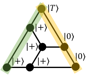 (b)
(b)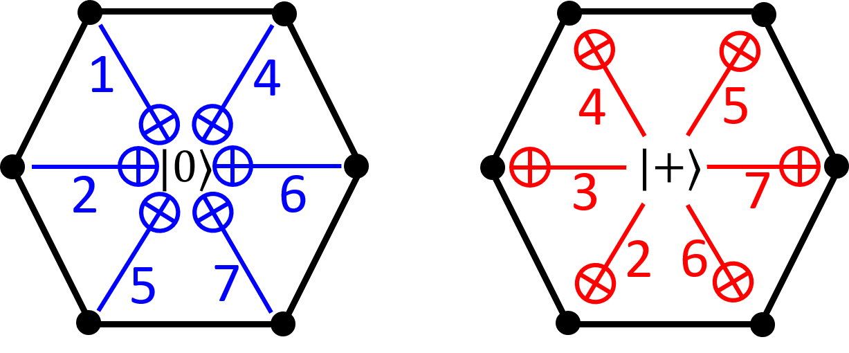 .
.
Lastly, we optimize the initialization protocol by varying the order in which the CNOT gates are applied during the two QEC rounds in step 2. We considered a range of system sizes, and again assume that there is a separate ancilla qubit per stabilizer generator and consider the valid schedules consisting of CNOT time units as in Section II.3. We found that the size resulted in the best parameters, and that the worst schedule (which is not the same as that used for standard error correction) results in more than twice the lowest-order failure probability of the best schedule; see Appendix C for more details.
The protocol takes
| (14) |
time units: one time unit to prepare the qubits in , and , and two QEC cycles each lasting 9 time units. We find that under circuit noise of strength the lowest order contributions to the output infidelity and rejection probability are
| (15) |
III.1.2 Expansion and movement of patches
We neglect any error introduced by expansion of the encoded states, i.e., while enlarging the distance of the base code from to between rounds and , and while these patches are moved into the starting location for the round. This is justified since errors are suppressed throughout the expansion similarly as during error correction of the distance- code. We also neglect any additional time overhead introduced by the expansion and movement of patches. This is justified since the expansion can be done within the QEC rounds, and the swaps needed to move the outputs each take just one QEC cycle, which we expect can be done during the QEC rounds needed to prepare the and states at the start of the state distillation circuit; see Fig. 21.
III.1.3 15-to-1 state distillation circuit
Here, we analyze the 15-to-1 scheme run on logical qubits encoded in patches of 2D color code with distance arranged in a 3D stack. The logical circuits are analysed using the effective noise model in Section II.4, which takes two parameters: the distance of the 2D color codes used, and the strength of the underlying circuit noise. Since we allow Clifford operations only between adjacent patches in the stack, we have to appropriately modify the state distillation circuit; see Fig. 21. In our analysis, we only keep track of errors up to order and , which are of similar order of magnitude in the regime of interest, where is the infidelity of the input encoded states, and is the noise strength in the effective noise model. This splits the analysis into looking at error either in the encoded states alone, or in the Clifford operations alone.
Noisy states.—First, we briefly review the effect of noise on states Bravyi and Kitaev 2005. As described in Section I.2, we simplify the form of noise assumed on a state by twirling, which in this case corresponds to randomly applying the Clifford with probability . Recall that single-qubit Clifford gates can be done instantaneously and perfectly by frame tracking in the 2D color code as described in Section I.4. This twirling forces the noisy state to be of the form , or equivalently that each state is afflicted by a error with probability . The noise on the set of input noisy states is therefore represented as a -type Pauli error occurring with probability . The protocol will reject if is a detectable error for the punctured Reed-Muller code, which has distance for -type operators. The protocol results in a failure if and only if is a nontrivial logical operator. Explicit enumeration shows that there are weight-3 -type logical operators, such that the contributions and due to errors are
| (16) |
Noisy Clifford operations.—Now we consider the effect of noise in the Clifford operations Jochym-O’Connor et al. 2013; Brooks 2013 in the state distillation circuit. First, we analyze the faults that occur during the Reed-Muller state preparation (lilac in Fig. 21), which takes 16 QEC cycles to complete. We propagate each fault as a logical Pauli operator through the circuit, and assume that every other operation acts perfectly, including the gates. By explicitly representing the state and operations as the vector and matrices of dimension and , respectively, we find that the contributions are
| (17) |
Next we consider faults in the 16 idle QEC cycles of the output qubit. Note that there is a choice of which of the 16 qubits of the Reed-Muller state to puncture in the 15-to-1 protocol. We simulated all 16 choices, and selected the third qubit as the output since it had the lowest contribution from ; see Appendix C. Any failure in any of these locations will result in an undetected failure
| (18) |
By explicit calculation, we find the exact contribution to and of every Clifford fault location in Fig. 21 according to our effective noise model.

Lastly we analyze the remaining fault locations. These consist of the idle locations involving qubits holding the states which remain idle during the production of the RM state (pink), the 420 idle and SWAP locations in the shuffle circuit (green), and the 15 CNOTs used to implement gate teleportation (blue) in Fig. 21. A single fault in any of these locations will propagate to a Pauli operator acting only on one pair of qubits as shown, where , , and each take values and the first qubit holds the , and the second is from the Reed-Muller state. To analyze the effect of such a Pauli operator, we imagine delaying the measurements on the affected pair of qubits until after the completion of the rest of the circuit; see Fig. 22. At this point, all other measurements are completed, and if the Pauli operator were trivial, i.e., if , the outcome of the measurement would be determined by the previous outcomes since the -stabilizers must be satisfied. Therefore, the pair of qubits must be completely unentangled with the rest of the system. This tells us that none of these fault locations can result in a failure, but result in rejection if and only if the outcome of the measurement is modified by the Pauli operator . We straightforwardly analyze this 2-qubit circuit with its pure initial state and for Pauli operator find the probability that the outcome is flipped, namely
Then all that remains is to count the contribution to each of these Paulis from the aforementioned locations according to the effective noise model, which yields
| (24) |
The contributions from Eq. (16), Eq. (17), Eq. (18) and Eq. (24) combine to give the rejection and failure probability of the state distillation step
| (25) | |||||
| (26) |
The number of time units required to implement the state distillation circuit can be straightforwardly identified from Fig. 21 and is equal to
| (27) |
III.2 State distillation overhead
Here we estimate the overhead required for a -round state distillation protocol using distances under circuit noise of strength , as well as the infidelities output by each round . Note that is the infidelity of the encoded state produced by the overall protocol.
Recall that the first step of the state distillation protocol is to initialize encoded states in distance- 2D color codes; see Fig. 19 and Section III.1.1. Writing the infidelity of the state after initialization as , the remaining infidelities are then calculated iteratively according to
| (28) |
To estimate the overhead, it is useful to streamline our notation. Recall from Eq. (12) that qubits are used to implement the distance- 2D color code. For each state distillation round , let be the acceptance probability, be the number of s required assuming acceptance, and be the number of logical qubits needed per input in the state distillation circuit. To account for the initialization step, we also set , , and .
We can calculate the expected number of physical qubits required in each round. We imagine preparing a large number of output states, and thus we can talk about the average overhead.77 7 If we were to produce just one output state, then the overhead would slightly increase as we would need to guarantee that with high probability there are sufficiently many states at each level of the state distillation protocol. Since the state distillation protocol in the last round succeeds with probability , on average it needs input s. We therefore require on average qubits for the last round. To supply the th round, the th round must therefore output ’s on average, which requires physical qubits, and so on. The qubit overhead of the state distillation protocol can then be found as the number of qubits needed in the most qubit-expensive state distillation round, namely
| (29) |
The time required for state distillation is
| (30) |
The space-time overhead is then simply . For various values of , we run a simple search over number of rounds and distances to distill a target infidelity for a low space or space-time overhead; see Fig. 23.
(a) (b)
Let us briefly remark on the threshold of this 15-to-1 state distillation using the 2D color code. This threshold is the noise strength above which arbitrarily low target infidelity cannot be achieved, irrespective of the number of state distillation rounds. There are two main features that could limit the state distillation threshold. Firstly, error correction in the 2D color code could be the limiting factor. Namely, if is above the circuit-noise threshold of , one will be unable to achieve logical states with arbitrarily low infidelity. Secondly, the first round of state distillation can be a bottleneck if the infidelity of the initial encoded state cannot be improved by it. For simplicity, we assume that the encoded Clifford operations execute perfectly, and solve for the critical infidelity satisfying . Using Eq. (15), we obtain a corresponding critical error rate of . We conclude that error correction is the bottleneck, so we estimate the threshold for state distillation with this scheme to be .
IV Further insights into 3D color codes
In this section we present some insights into 3D color codes that are useful for code switching. In Section IV.1, we describe a simple approach to switch between the 2D and 3D color codes. At the core of this approach is the fact that in a particular state of the gauge qubits, the 3D subsystem color code can be viewed as a collection of 2D color codes. In Section IV.2, we describe some relevant features of the gauge operators of the 3D color code which will be relevant for gauge-fixing and also for the simulation of noise upon the application of the transversal gate. Our discussion closely follows material in Bombin 2018b. In Section IV.3, we generalize the restriction decoder to correct -errors in the 3D color code with boundaries, which will later be used in our code switching protocol.
IV.1 A simple way to switch between 2D and 3D color codes
First we recall the general procedure for gauge fixing from a subsystem code with gauge group to a stabilizer code with stabilizer group , where both codes share a set of bare logical operators. We require that the stabilizer group of the subsystem code, which is the centralizer of in the Pauli group intersected with modulo the phase, i.e., , is contained in , namely . Consider any state in the code space of the subsystem code, which by definition is a -eigenstate of all elements of . To switch from to , we first measure a generating set of . A subset of those measured generators may have outcomes, but there must exist an element which anti-commutes with precisely that subset of generators. Hence after applying , all the stabilizers of will be satisfied, and since commutes with the bare logical operators, the logical state is unaffected, which completes the transfer from to . This procedure is named gauge fixing since it involves measuring some (initially unsatisfied) gauge operators, and fixing them to be .
Central to switching between color codes is the fact that both the 3D stabilizer color code and the 2D color code can be viewed as gauge fixings of the 3D subsystem color code; see Fig. 24. The gauge and stabilizer groups and for the 3D subsystem color code, and the stabilizer group for the 3D stabilizer color code are:
| (31) | |||
| (32) |
We can define the stabilizer group of the 2D color code within the 3D lattice since is ‘contained’ in ; see Fig. 24(b). Namely,
| (33) |
where is the boundary vertex. Let us define the stabilizer group supported on the qubits which are not near as follows
| (34) |
We can think of as the group generated by the stabilizers of the 2D spherical color codes centered around every interior vertex of ; see Fig. 24(c). Note that every 2D spherical color code encodes zero logical qubits.
(a) (b)
(b)
 (c)
(c)
It is straightforward to see that contains both and . Moreover, and since vertex operators and can be formed by multiplying operators and on all the edges of the same color incident to . Also note that there is a shared representation of bare logical operators for all three codes (for example and applied to every qubit in ). Therefore, to move from the subsystem code to either of the stabilizer codes, i.e., or , gauge switching can be used. Switching from either of the stabilizer codes to the subsystem code requires no action, since any state which is a -eigenstate of every element of or must also be a -eigenstate of every element in .
This example of gauge fixing is sometimes referred to as a dimensional jump because the logical information is moved between codes defined on 2D and 3D lattices Bombín 2016.
IV.2 Physics of the gauge flux in 3D color codes
Here we consider general features of the gauge operators of the 3D subsystem color code. Our discussion closely follows material in Bombin 2018b. Suppose there is some error in the system. We define the -type gauge flux to be the subset of interior edges which would return outcomes if all edges in the system were measured perfectly. Since each edge has one color from , we distinguish six types of the flux and write
| (35) |
(a) (b)
(b)
Although the flux can be random, it has to form a collection of strings, which may branch and can terminate only at the boundary of the lattice; see Fig. 25. A local constraint capturing this behavior, which we call the Gauss law, can be stated as follows. Let be four different colors. Then, for any vertex of color , the number of edges of of color or and incident to has to be even, i.e.,
| (36) |
This local constraint arises from the redundancies among gauge generators. Namely, in order to form a stabilizer generator identified with the vertex , we can multiply all the gauge generators on edges of color incident to . Alternatively, we can obtain as the product of all gauge generators on edges of color incident to . Since the parity of the number of measurement outcomes among those gauge generators in both cases is the same, we recover Eq. (36).
Note that when the stabilizer is violated (indicating the presence of some error), then the number of outcomes for gauge generators on edges incident to of color has to be odd, i.e., . In such a case, we call the vertex a branching point of , as three different flux types , and meet at . We remark that to perform error correction with the 3D subsystem color code, one can use the information about the branching points of the flux . If the flux has no branching points at any interior vertex, then all stabilizers are satisfied and there always exists an -type gauge operator which anti-commutes with precisely those gauge generators in .
If an edge set satisfies the Guass law, we say that it is valid. An edge set which does not satisfy the Gauss law is said to be invalid, and we refer to all vertices which violate the Gauss law as violation points. When the gauge flux is measured with noisy circuits, there can be errors in the reported noisy gauge flux causing it to be invalid; see Fig. 26.
(a) (b)
(b)
Now, we discuss the structure of the flux which satisfies the Gauss law. First, we can find a decomposition of in terms of its connected components, i.e.,
| (37) |
By definition, different connected components are disjoint, i.e., for .
Then, we define a linked component of as a subset of all connected components of , which are linked (in the sense of knot theory); see Fig. 25(b). Finally, we can decompose as a disjoint union of its linked components
| (38) |
Note that each is the sum of some ’s.
For convenience, we introduce a function , which for each vertex returns its color, where we set , , and .
For any linked component of we refer to a subset as an excitation configuration for and call the total charge of . We denote the collection of excitation configurations for with the neutral total charge as follows
| (39) |
Writing the linked component in terms of its connected components , we also introduce the collection of excitation configurations without the linking charge
| (40) |
We remark that the linking charge is a charge which can be transferred between two connected components and , which are linked; see Bombin 2018b. Note that is contained in , i.e., , and they coincide whenever the linked component consists of a single connected component.
IV.3 Restriction decoder for 3D color codes with boundaries
Here we provide details on correcting type errors in the 3D stabilizer color code with perfect measurements, which is needed for the final step of the code switching protocol. We seek an efficient decoder for the 3D color code with good performance. Our approach is to adapt the restriction decoder from Ref. Kubica and Delfosse 2019, which was originally defined for lattices with no boundary, to the tetrahedral lattice . We also apply additional minor modifications to improve the performance. In what follows we briefly review the restriction decoder and describe our modifications.
Let be the syndrome of the 3D stabilizer code on the tetrahedral lattice . We pick one color, say , and for each color we separately analyze the restricted syndrome within the restricted lattice . If , then we add the boundary vertex to . Next, we find a subset of edges , which provides a pairing of vertices of within the restricted lattice . Note that we can find a pairing of minimal weight by using the MWPM algorithm. Also, the weight of the edge connecting the boundary vertices and is set to zero.
After finding the pairing we apply a local lifting procedure to every vertex in the interior of . Namely, for every vertex we find any subset of tetrahedra in the neighborhood of , whose -boundary locally matches , i.e., . We emphasize that all such choices of result in operators , which may differ only by a stabilizer operator.
To lift the boundary vertex , we need to adapt the original restriction decoder from Ref. Kubica and Delfosse 2019. Since is a sublattice of (see Fig. 24(b)), one can show that the problem of finding , which satisfies , is equivalent to the problem of decoding the 2D color code defined on the facet of the tetrahedral lattice near . We remark that different choices of may lead to operators differing by a logical operator. We use the projection decoder for the 2D color code as described in Section II.1. Finally, the correction operator is found as , where the product is over all vertices, including the boundary vertex . Note that this adaption to accommodate a lattice boundary in 3D is analogous to an adaption presented in Chamberland et al. 2020b for the 2D case.
In Fig. 27(a) we show the performance of the restriction decoder adapted to the 3D stabilizer color code on the tetrahedral lattice , finding a threshold of for independent and identically distributed (iid) phase-flip noise. This value can be contrasted with the restriction decoder threshold of for the color code on the -torus reported in Kubica and Delfosse 2019. Also, a similar adaption of the restriction decoder to the 3D color code with a boundary was recently presented in Turner et al. 2020, however the reported values of – are surprisingly low.
This adapted restriction decoder on moderate system sizes is far from optimal. For example, some weight-2 errors can cause failure for any . This phenomenon is not solely due to the presence of the boundaries. Namely, we found that there are some weight- errors in the color code of distance on the -torus, which cause the restriction decoder to introduce a logical error.
To improve the performance, we consider a very simple additional modification of the restriction decoder to improve its performance for moderate system sizes. In addition to selecting a small weight set for the boundary vertex , we choose as the set of minimal weight for every vertex . As mentioned above, this can only change the decoder output by a stabilizer, but the explicit representation will typically be of lower weight. Then, we simply rerun the same decoder three times by picking other colors, i.e., , and instead of , and finally select the correction which has the lowest total weight among the four for colors , , , and . This simple modification yields significant improvements: the lowest distance which corrects all weight-2 errors is now compared to which was needed without the modification, and the threshold is increased from to ; see Fig. 27.
(a) (b)
V Code switching analysis
In this section we describe how code switching between 2D and 3D color codes can be used to fault-tolerantly produce an encoded state in the 2D color code, and analyze the overhead of this process.
V.1 Creating the T state via code switching in 6 steps
Here we outline the protocol to produce an encoded state using code switching in the presence of circuit noise. The main idea is to first produce a Bell state across a pair of 2D color codes, and switch one of the two into a 3D color code where the logical is applied transversally. Then, by measuring for the 3D code, the encoded state is effectively teleported to the remaining 2D code (up to a known logical Pauli correction). This approach avoids switching from the 3D code back to the 2D code, which we believe considerably reduces the amount of extra noise and simplifies our simulation. More explicitly, the protocol consists of the following steps (which are illustrated in Fig. 28).

- 1.
Prepare Bell state in 2D codes.—The encoded Bell state state is fault-tolerantly prepared in a pair of 2D color codes, defined on two copies of the lattice . The second of these 2D color codes should be seen as the code defined along the 2D boundary near the yellow vertex of the 3D lattice as in Fig. 24(b).
- 2.
Prepare the 3D interior.—The remaining qubits in , i.e., those which are not near the boundary vertex , are prepared as a tensor product of unique spherical 2D color code states. The logical state of the system is a Bell pair between a 2D color code and the 3D subsystem color code .
- 3.
Measure gauge operators.—All -edge operators for all edges not incident to any vertex are measured, yielding the subset of edges corresponding to outcomes.
- 4.
Gauge fix.—We find and apply an -gauge operator which seeks to fix all -edge operators to have +1 outcomes. The logical state is now a Bell state encoded into the 2D color code and the 3D stabilizer color code .
- 5.
Apply , and measure.—We apply to every data qubit. This, in turn, implements a logical gate, yielding the state . Then we measure each individual data qubit in the 3D code in the basis.
- 6.
Decode errors in 3D code.—We use the single-qubit -basis measurements to first decode -errors, and then infer the outcome of the logical . Then, the state encoded in the 2D color code is , which for needs to be fixed to the encoded state by application of logical .
In the following subsections, we go through each of the six steps, elaborating on the implementation and simulation details. In our analysis, we adhere to the following guiding principles.
- •
For each step, we use Monte Carlo simulations under circuit noise to estimate the performance. We select the best error correction techniques, fault-tolerant gadgets and efficient decoding algorithms that we are aware of, and optimize measurement circuits where possible.
- •
It is possible that some steps will benefit from future improvements in error correction techniques and decoders. We estimate the impact these could have on the performance of this code switching protocol by replacing those steps by a justified estimate of the best improvement one could hope for.
- •
We choose the fault-tolerant error correction for the 2D color code to be the same optimized configuration we assumed for state distillation (see Section II.4) to allow for a fair comparison between code switching and state distillation.
- •
We assume a single ancilla qubit per gauge operator in the 3D color code interior.
In Fig. 29(a) we present our findings by showing the overall probability of failure of code switching using our simulations. In Fig. 29(b)-(f) we indicate the impact of optimistic improvements of various steps in the protocol on the overall probability of failure of code switching.
(a)
(b)
(c) (d)
(e) (f)
V.1.1 Preparing the Bell state in 2D codes
To fault-tolerantly prepare the encoded Bell state in a pair of 2D color codes of distance , we first fault-tolerantly prepare them in and respectively, and then transversally apply a CNOT from the first to the second. Preparation of is carried out by initializing all data qubits in the 2D color code in , and then performing QEC cycles and fixing the inferred initial syndrome of the stabilizers. Preparation of similarly involves initialization of all data qubits in , followed by QEC cycles and fixing the inferred initial syndrome of the stabilizers. Since each QEC cycle for the 2D color code requires 8 time units, the preparation of the encoded Bell state takes time units. After this point the second of the 2D codes undergoes a single additional QEC cycle while code switching occurs for the first 2D code patch. Although it is arbitrary which of the two patches is used for code switching, in practice there is an asymmetry in the and noise for the patches. We find a marginal benefit from feeding the first patch (initialized in prior to the CNOT) to be used for code switching. For details, see Appendix E.
V.1.2 Preparing the 3D interior
There are 2D spherical color code states to be prepared around each yellow vertex as that shown in Fig. 24(b). Implementation details and optimizations of this step are given in Appendix D and Appendix E, but we provide the key features here.
Data qubits are prepared in , then stabilizers are measured with the shortest circuit that uses a single ancilla. If the syndrome extracted for a 2D color code around a yellow vertex is valid, meaning there is an operator that will set all stabilizers to have outcomes, then such a fix is applied, otherwise the preparation is repeated. If the second iteration also yields an invalid syndrome, one randomly selected outcome is flipped, producing a valid syndrome which is then fixed. The interior preparation step is started sufficiently early so that any repeated preparations have finished by the time the two 2D color code patches completes. Note that since the 2D spherical color code encodes no logical qubits, it is not necessary to repeat measurements, in contrast to preparation of a logical state in the 2D color code patch, which requires a number of QEC cycles proportional to .
Optimistic improvements. One may hope to improve the preparation of the 2D spherical color codes. Although we found a schedule of shortest length to measure the stabilizers, there could be many others of the same length which could potentially lead to fewer errors. Moreover, it may be possible to exploit the unused ancilla associated with the , and edges and to consider collective rather than independent preparations of the 2D color codes. No matter how good such a preparation protocol is, it would require at least three time units as each qubit appears in three -type stabilizer generators. Therefore, we use three idle time units with circuit noise of strength to bound potential improvements of this step in Fig. 29(b).
V.1.3 Measuring gauge operators
To change gauge to the 3D stabilizer code, the -edges of color in are measured. Implementation details and optimizations of this step are given in Appendix F. We find a minimal length circuit to measure the gauge operators in parallel with a single ancilla qubit per edge. Including ancilla preparation and measurement, this circuit requires 8 time units, although the preparation can be done during the last time unit of the interior preparation step.
Since we choose to measure only -edge operators of color in , not all -edge operators, we only learn the restricted noisy gauge flux . We emphasize that due to faults in the measurement process, is likely to violate the Gauss law and differ from the restricted gauge flux in the system.
Optimistic improvements. It seems difficult to reduce the errors introduced by this step without increasing the space or time overhead significantly, and for example to use verified cat states to measure each edge operator. We will neglect any space or time overhead in our estimate so that we bound the effect of potential improvements. As each data qubit is in three measurements, a minimum of three time units would be required to implement the measurement. Therefore, we use three idle time units with circuit noise of strength in our optimistic simulation in Fig. 29(c).
V.1.4 Gauge fixing
This step corresponds to a classical algorithm which takes as its input the restricted noisy gauge flux corresponding to some subset of edges of color in , and outputs some -type gauge operator aiming to fix . The algorithm proceeds as follows.
- (i)
Validation of the noisy flux: for any color we validate the noisy restricted flux by matching its violation points within the restricted lattice . We denote by the set of edges used in the pairing of the violation points of . Then, is the validated flux. Note that .
- (ii)
Gauge-fixing from the validated flux: we find an operator consistent with and apply it. Such an -gauge operator can be efficiently found by e.g. Gaussian elimination.
In this step, we are treating the restricted noisy gauge flux as arising from a gauge flux with no branching points along with some measurement errors; see Fig. 30. In other words, we want to find a gauge flux corresponding to some -gauge operator just by looking at its restricted noisy gauge flux . However the gauge flux can in fact have branching points due to errors in the system. In such a case, the restricted noisy gauge flux does not even satisfy the Gauss law in the absence of measurement errors as we omit -type operators associated with , and edges. For every we choose to independently pair up all the violation points of within the restricted lattice , which in turn allows us to find the desired .
(a) (b)
(b)
Optimistic improvements. One can ask how close to optimal the performance of the algorithm is. For instance, it may be possible to not only estimate a gauge fix from the noisy -flux measurement, but also to correct errors in the system; see Fig. 30. To bound the impact of any potential improvements of this step in our simulation, we assume that all errors in the system prior to the gauge measurements are corrected, and that the gauge itself is identified exactly; see Fig. 29(d). The only remaining error that is retained in this bound is therefore that which is introduced by the noisy gauge measurement circuits themselves.
V.1.5 Applying T and measuring the 3D code’s data qubits
In this step, we first apply the gate to each data qubit, and then measure it in the basis. These can be combined into a single operation requiring one time unit. Despite being one of the simplest code switching steps to implement, it is quite challenging to simulate efficiently due to the large number of gates. In what follows we describe how we exploit some additional structure and assumptions that render the simulation tractable.
Let the -type residual error before the application of the logical gate be supported on ; similarly, let denote the -type residual error. Note that if we could perfectly fix the gauge in the previous step and there were no additional -errors, then there would be no residual -error. Generically, there is some nontrivial residual -error, which unlike the -error does not commute with the logical gate. The effect of the residual -error on the measurement outcomes amounts to, roughly speaking, flipping some outcomes along the -gauge flux of the the residual -error . This is made precise in the following lemma.
Lemma V.1.
Let be residual - and -errors. Let be the -gauge flux and be a decomposition of into its linked components ’s. If is applied to every data qubit and the stabilizers are perfectly measured, then one obtains a syndrome
| (41) |
where each excitation configuration is chosen uniformly at random from .
In above, we use notation introduced in Section IV.2. To simulate this step, one can generate Pauli operators resulting in the same distribution of syndromes. Note that there is a possibility of introducing a logical operator at this step, which we ignore in our simulation, leading to an underestimate of the failure of code switching. For more details and a justification of this lemma, see Ref. Bombin 2018b.
In our simulation we make the additional simplifying assumption to sample uniformly from within the collection of excitation configurations without the linking charge rather than the collection of excitation configurations . Recall that . This assumption amounts to ignoring the linking charge, and we do not expect it to substantially effect the performance. We generate the random -error as
| (42) |
where is a local sampling procedure, which we now describe in detail. Let be a vertex of color , which is incident to the flux , and be the restriction of to the edges incident to . Let denote the set of three different colors. We find a subset of tetrahedra containing as follows.
- (i)
With probability set ; otherwise .
- (ii)
For each , if , then choose uniformly at random a subset of even cardinality; otherwise choose uniformly at random a subset of odd cardinality.
- (iii)
Find a subset of tetrahedra , whose -boundary locally matches , i.e.,
(43)
We now explain why this algorithm produces with the correct syndrome distribution. First, any excitation configuration can be viewed as a sum of local excitation configurations with neutral total charge. If the vertex is in , then step (ii) is equivalent to randomly selecting a local excitation configuration for , which is created by operators supported within the neighborhood of and with the neutral total charge. Since each local excitation configuration is equally likely selected, thus the resulting excitation configuration is chosen uniformly at random from . Also note that the search in (iii) can be implemented by exhaustively checking which of the possible subsets of tetrahedra containing satisfies Eq. (43). This naive implementation is nevertheless efficient since is bounded. Lastly, we remark that the residual -error present in the system right before the measurement in the basis is . We use this -error in the following code switching step.
V.1.6 Decoding Z errors in the 3D color code
In the final step of the protocol, a classical decoding algorithm is run to correct errors for the 3D stabilizer color code. The input to the decoder is the set of measurement outcomes for each data qubit from the previous step. The output of the decoder will be a -type Pauli correction which, if applied, would flip all the syndromes computed given the single-qubit outcomes. At that point one can reliably read off the logical measurement . Then, the state encoded in the remaining 2D color code from step 1 is , which is the encoded state, up to the multiplication by for .
We implement a decoder based on the restriction decoder from Ref. Kubica and Delfosse 2019, but modified in two ways. The first modification is to adapt the decoder to the 3D stabilizer color code on the lattice which has boundaries. The second modification is to improve performance. We do this by favoring low-weight corrections (which differ by a stabilizer from the output of the original decoder). Running four independent versions of this decoder in parallel, we then simply select the lowest-weight correction from the four candidates. We describe and analyze the performance of this modified restriction decoder in Section IV.3.
Optimistic improvements. A different decoder may improve the performance of code switching. It is difficult to give as rigorous bounds on the performance of this step as we were able to give for the previous steps. However, by assuming that the best decoder performs as if the phase-flip noise was iid, we estimate the effect of any potential performance improvements using the following steps:
- (i)
Run the modified restriction decoder, and if it succeeds then we assume the improved version would also succeed, if it fails then continue to the next step.
- (ii)
Let be the minimum of the weight of the error, and the weight of the correction produced by the modified restriction decoder. Let be the number of data qubits in the distance- 3D stabilizer color code. Choose uniformly at random a real number from to , and if it is smaller than , then the correction fails; otherwise, the correction succeeds.
Note that is the known threshold of the optimal decoder for the 3D stabilizer color code under iid noise Kubica et al. 2018. We provide more detailed justifications for this estimate in Appendix G. The impact of potential improvements of this step on code switching is shown in Fig. 29(e).
V.2 Code switching overhead
To calculate the space and time overhead required to produce an encoded state with failure probability , we first find the minimum distance which achieves this by extrapolating the data in Fig. 29(a). The time to implement the code switching protocol at distance is simply , which is the time for QEC cycles of the 2D color code to complete. The number of qubits to implement the code switching protocol at distance is
| (44) |
This is comprised of two 2D color code patches (each of which has qubits from Eq. (12)) and the 3D interior (which has data qubits and measurement qubits). Details of the lattices which make clear where these numbers originate from can be found in Appendix A.
In Fig. 29 we fit a special form of the ansatz in Eq. (7), i.e., to fit the data up to the crossing. Setting the failure probability to be at most the target infidelity, i.e. , and solving for we obtain
| (45) |
where we round the right hand side up to the closest odd integer. Finally, in Fig. 31 we substitute this into and plot the qubit overhead and the space-time overhead as a function of for various values of for two cases: assuming no improvements, and assuming all optimistic improvements can be achieved.
(a) (b)
VI Discussion and Acknowledgments
In this work, we have simulated concrete realizations of state distillation and code switching under circuit noise and compare the overhead that each requires to produce high-fidelity states encoded in 2D color codes. We have focused on regimes of practical interest, with physical error rates from to and target logical error rates from to ; see Fig. 2. For error rates of and above, our implementation of code switching is not viable since its observed threshold was , considerably lower than that of for state distillation. For error rates near , our implementation of code switching becomes viable, but requires considerably more overhead than state distillation. However for error rates around , our code switching implementation begins to slightly outperform that of state distillation. Lastly, we see in Fig. 2 that a highly-optimistic implementation of code switching (which may be very difficult if not impossible to achieve) would not provide substantial savings over our simple implementation of state distillation in the studied regimes.
We now discuss the scaling of the space overhead and space-time overhead of code switching and state distillation for small physical error rate, i.e., . We further assume that . As we show in Appendix H, we have
| (46) |
where and are some constants, for code switching and for state distillation. Here, is the ratio of the number of input to output magic states and is the order of error suppression in a single distillation round. The change in the value of can be understood as follows—if , then the overhead is dominated by the initial distillation round; otherwise, it is dominated by the final round. For the 15-to-1 distillation scheme we have and , leading to and . From Eq. (46) we thus conclude that for state distillation will always outperform code switching. On the other hand, if we are willing to extrapolate Eq. (46) to more modest values of , the overhead of code switching is predicted to drop below that of state distillation. The precise value of the crossover is highly sensitive to the implementation details, but this could explain why we observe code switching outperforming state distillation for low and modest in Fig. 2.
Our findings point toward a number of future research directions. First, it could be fruitful to explore the potential of code switching in the regime of very low error rates, which may be achievable in trapped ion qubits Bruzewicz et al. 2019 and topological qubits Karzig et al. 2017. Second, improving the 2D color code state preparation procedure, syndrome extraction, and decoding algorithms would further reduce the overhead of both code switching and state distillation. We expect that code switching may also greatly benefit from better 3D color code decoders. Third, our code switching protocol produces the state, but it is possible to directly apply the gate rather than injecting it which may allow one to implement code switching in constant time rather than a time which scales with the code distance . Fourth, we have seen that in contradiction with the commonly held belief that a distillation scheme overhead is dominated by that of the first round , the last round overhead is when implemented with 2D codes, and dominates when . This suggests that searches and optimizations of new distillation schemes should not be restricted to those with very low .
Acknowledgments.— M.E.B. acknowledges relevant scientific discussions with many researchers from the QEC community, including Thomas Bohdanowicz, Héctor Bombín Ben Brown, Earl Campbell, Nicolas Delfosse, Austin Fowler, Jeongwan Haah, Tomas Jochym O’Connor, Cody Jones, Andrew Landahl, Ying Li, Michael Newman, John Preskill, and Marcus P da Silva. He is especially grateful for the encouragement for this project from David Poulin. M.E.B. also wishes to thank Achiamar Lee Rivera for her unwavering support throughout this research. A.K. is deeply indebted to Héctor Bombín for many colorful discussions. A.K. acknowledges funding provided by the Simons Foundation through the “It from Qubit” Collaboration. Research at Perimeter Institute is supported in part by the Government of Canada through the Department of Innovation, Science and Economic Development Canada and by the Province of Ontario through the Ministry of Colleges and Universities. This work was completed prior to A.K. joining AWS Center for Quantum Computing.
Appendices
A Lattice parameters and specifications
Here we provide parameters of the lattices which are used throughout the paper. Table 2 and Table 3 show parameters of the direct lattice and the dual lattice used to define the 2D and 3D color codes of distance . In general, these lattices can be obtained by tessellating a -sphere with -simplices and then removing one vertex from that tessellation, as well as all the simplices containing that vertex Kubica and Beverland 2015; Bombin 2015a.
| # vertices | # incident faces |
|---|---|
| 4 | |
| 6 | |
| 3 |
| # vertices | # incident tetrahedra | # edges | # incident tetrahedra |
|---|---|---|---|
| 4 | 6 | ||
| 8 | 4 | ||
| 12 | 6 | ||
| 18 | |||
| 24 |
B Supplementary details for 2D color code simulations
Here we provide additional data for the analysis of the performance of the 2D color code using the faulty-measurement projection decoder under phenomenological noise and circuit noise in Section II. In Fig. 32 we show the performance under phenomenological noise, which we use to produce the long-time pseudo-threshold plot in Fig. 11(d) in the main text. Similarly, in Fig. 33 we show the performance under phenomenological noise, which we use to produce the long-time pseudo-threshold in Fig. 13(b) in the main text. We point out that the decay parameter in the fit of the time-dependent pseudo-threshold in Fig. 32(b) and Fig. 33(b) shows that convergence to the long-time pseudo-threshold seems not to depend significantly on the system size. In Fig. 34 we provide the data used to produce the crossings in Fig. 13(b). In Fig. 35 we show the impact of optimizing the stabilizer extraction circuit on the performance of error correction under circuit noise. In Fig. 36, we show additional data from which we extract the logical failure rates for in Fig. 16(b) in the main text.
(a) (b)
(a) (b)
(a) (b) (c)
(a) (b)
C Supplementary details for distillation analysis
Here we provide more details of the distillation analysis in Section III. In Table 4 we consider variants of the distillation circuit formed by puncturing different qubits of the quantum Reed-Muller state. This helps us identify that puncturing qubit number three is best with the noise model we assume in this paper since it results in the smallest leading order failure probability given that .
| punctured qubit | failure probability | rejection probability |
|---|---|---|
| 1 | ||
| 2 | ||
| 3 | ||
| 4 | ||
| 5 | ||
| 6 | ||
| 7 | ||
| 8 | ||
| 9 | ||
| 10 | ||
| 11 | ||
| 12 | ||
| 13 | ||
| 14 | ||
| 15 | ||
| 16 |
Now we elaborate on the procedure to initialize a state in a distance color code described in Section III.1, and explain some structure that we exploit to simplify the noise analysis. First note that even in the absence of noise, the stabilizers which are measured in the initialization protocol have uncertain outcomes because the state is not a code state of the 2D color code at the start of the protocol. Let and be the two sets of qubits prepared in and , respectively; see Fig. 20(a). The protocol involves taking the observed syndrome , and producing a Pauli operator , where and are Pauli and operators supported on qubits in and , respectively. The protocol rejects if no such fix exists or if the syndromes from the consecutive rounds of QEC differ . Note that the fix is unique up to a stabilizer since neither of the disjoint sets and support a logical operator. This implies that for any two syndromes and the Pauli operators and are equivalent up to a stabilizer.
To faithfully simulate this protocol in the presence of noise, one can consider the scenario in which a complete set of perfect stabilizer measurements is performed (and their outcomes discarded) before the QEC circuits are applied. This allows us to begin the simulation with a state, which is an eigenstate of the stabilizer group. The simulation can therefore be implemented as follows.
- 1.
Start with a perfect code state.
- 2.
With some probability , apply a Pauli operator , where and are Pauli and operators supported within and , respectively.
- 3.
Run the noisy circuits explicitly as described in Section I.2. A set of faults will propagate to some Pauli error on the data qubits at the end of the protocol. The faults could result in the syndromes from the two QEC cycles disagreeing, in which case the protocol is rejected, or both QEC rounds having the same observed syndrome , possibly different from the syndrome of . Note that can only depend on the set of faults, and is independent of .
- 4.
Apply a Pauli operator with the syndrome , where and are Pauli and operators supported on qubits in and , or reject if such an operator cannot be found.
- 5.
If the net operator is correctable, then we say that the protocol succeeds, and otherwise we say it fails.
However, note that the net operator must be independent of , since and are equivalent up to a stabilizer. In our simulation we therefore set to be trivial for simplicity without loss of generality.
Using this simulation approach, we analyze all 234 valid CNOT schedules for a variety of distances, and find that as shown in Fig. 20 has the lowest failure pro ability, namely . For comparison, the worst schedule using was and would result in a of .
D Preparing the 3D interior for code switching
Here we consider the 3D interior of the initial state for code switching discussed in Section V.1.2, which consists of a (trivial) 2D color code state on the qubits surrounding each interior vertex. This object can be viewed as a 2D sphere; see Fig. 37. This state of each sphere is formed by preparing all data qubits in the state, then measuring the stabilizers, each with an ancilla measurement qubit in a single QEC cycle, followed by the application of an appropriate Pauli to fix incorrect stabilizers.

(a)
 (b)
(b)
 (c)
(d)
(c)
(d)
CNOT circuits.—For each of the four types of spheres, we find an ordering of CNOTs which allows for a minimal-length circuit to measure the stabilizers; see Table 5. These sequences were found using a greedy algorithm with a random initial sequence and minimizing the cost function of the number of unsatisfied constraints (we require that no qubit is involved in more than one gate per time unit) minus the average time unit when each gate occurs. The greedy algorithm terminates when all constraints are satisfied and when the cost function cannot be further reduced. We fixed the total number of time units to be minimal (4 CNOT time units for the 8-qubit sphere, which involves only weight-4 stabilizers, and 6 CNOT time units for the 12-, 18- and 24-qubit spheres, which involve weight-6 stabilizers). We maximize the average time unit when each gate occurs since this removes idle time units by not preparing ancillas for lower-weight stabilizer measurements until they are needed. The sequences we found are optimal with regard to this cost function: all constraints were satisfied using the minimal number of time units, and all weight- stabilizer generators have CNOTs in the last time units of each schedule. There could be many schedules which are optimal in this sense, but we did not attempt to explore among those for schedules which performed better.
To make the representation of the schedules slightly more compact, we specify 17 vertex locations in a list in lexicographical order as follows
| (47) | |||||
where the coordinates and are for placing boundary vertices and , while the others describe the interior vertices. The colors of the vertices in in order are , , , , , , , , , , , , , , , , . The central vertex is placed at the origin and is the eighth entry in . To apply the CNOT schedules we specify in Table 5, one must map the neighborhood of every vertex to one of these four standard configurations. All interior vertices lie precisely on these standard coordinates relative to their central yellow vertex. Boundary vertices connected to their central yellow vertex will not be on the standard coordinates in , but can be identified and shifted to the standard coordinate uniquely since there is at most one boundary vertex of each color included in the neighborhood of any yellow vertex.
| sphere size | edge | time unit 1 | time unit 2 | time unit 3 | time unit 4 | time unit 5 | time unit 6 |
|---|---|---|---|---|---|---|---|
| (8,1) | (1,2,4,8) | (1,2,3,8) | (1,3,8,17) | (1,4,8,17) | |||
| (8,2) | (1,2,3,8) | (1,2,4,8) | (2,3,8,15) | (2,4,8,15) | |||
| 8 | (8,3) | (3,8,15,17) | (2,3,8,15) | (1,2,3,8) | (1,3,8,17) | ||
| qubits | (8,4) | (2,4,8,15) | (4,8,15,17) | (1,4,8,17) | (1,2,4,8) | ||
| (8,15) | (2,3,8,15) | (2,4,8,15) | (4,8,15,17) | (3,8,15,17) | |||
| (8,17) | (1,3,8,17) | (1,4,8,17) | (3,8,15,17) | (4,8,15,17) | |||
| (8,1) | (1,3,8,17) | (1,2,3,8) | (1,2,4,8) | (1,4,8,17) | |||
| (8,2) | (1,2,3,8) | (1,2,4,8) | (2,3,6,8) | (2,6,8,11) | (2,4,7,8) | (2,7,8,11) | |
| (8,3) | (1,2,3,8) | (2,3,6,8) | (1,3,8,17) | (3,6,8,17) | |||
| 12 | (8,4) | (1,2,4,8) | (2,4,7,8) | (1,4,8,17) | (4,7,8,17) | ||
| qubits | (8,6) | (6,8,11,17) | (3,6,8,17) | (2,3,6,8) | (2,6,8,11) | ||
| (8,7) | (2,7,8,11) | (7,8,11,17) | (4,7,8,17) | (2,4,7,8) | |||
| (8,11) | (2,6,8,11) | (2,7,8,11) | (6,8,11,17) | (7,8,11,17) | |||
| (8,17) | (1,3,8,17) | (1,4,8,17) | (3,6,8,17) | (4,7,8,17) | (7,8,11,17) | (6,8,11,17) | |
| (8,1) | (1,2,3,8) | (1,2,4,8) | (1,3,5,8) | (1,4,5,8) | |||
| (8,2) | (1,2,4,8) | (1,2,3,8) | (2,3,8,15) | (2,4,8,15) | |||
| (8,3) | (1,2,3,8) | (1,3,5,8) | (3,5,8,9) | (2,3,8,15) | (3,8,9,12) | (3,8,12,15) | |
| (8,4) | (1,2,4,8) | (1,4,5,8) | (4,5,8,10) | (2,4,8,15) | (4,8,10,13) | (4,8,13,15) | |
| 18 | (8,5) | (1,3,5,8) | (3,5,8,9) | (1,4,5,8) | (4,5,8,10) | (5,8,9,14) | (5,8,10,14) |
| qubits | (8,9) | (5,8,9,14) | (3,8,9,12) | (3,5,8,9) | (8,9,12,14) | ||
| (8,10) | (4,8,10,13) | (5,8,10,14) | (4,5,8,10) | (8,10,13,14) | |||
| (8,12) | (3,8,9,12) | (3,8,12,15) | (8,9,12,14) | (8,12,14,15) | |||
| (8,13) | (8,13,14,15) | (4,8,13,15) | (8,10,13,14) | (4,8,10,13) | |||
| (8,14) | (5,8,9,14) | (5,8,10,14) | (8,9,12,14) | (8,10,13,14) | (8,12,14,15) | (8,13,14,15) | |
| (8,15) | (2,4,8,15) | (3,8,12,15) | (4,8,13,15) | (8,12,14,15) | (8,13,14,15) | (2,3,8,15) | |
| (8,1) | (1,2,3,8) | (1,2,4,8) | (1,3,5,8) | (1,4,5,8) | |||
| (8,2) | (1,2,3,8) | (1,2,4,8) | (2,6,8,11) | (2,3,6,8) | (2,4,7,8) | (2,7,8,11) | |
| (8,3) | (2,3,6,8) | (1,2,3,8) | (1,3,5,8) | (3,5,8,9) | (3,8,9,12) | (3,6,8,12) | |
| (8,4) | (1,2,4,8) | (2,4,7,8) | (1,4,5,8) | (4,7,8,13) | (4,5,8,10) | (4,8,10,13) | |
| (8,5) | (1,3,5,8) | (1,4,5,8) | (3,5,8,9) | (4,5,8,10) | (5,8,9,14) | (5,8,10,14) | |
| (8,6) | (2,3,6,8) | (2,6,8,11) | (3,6,8,12) | (6,8,11,12) | |||
| 24 | (8,7) | (2,4,7,8) | (2,7,8,11) | (4,7,8,13) | (7,8,11,13) | ||
| qubits | (8,9) | (3,8,9,12) | (5,8,9,14) | (3,5,8,9) | (8,9,12,14) | ||
| (8,10) | (4,5,8,10) | (4,8,10,13) | (5,8,10,14) | (8,10,13,14) | |||
| (8,11) | (2,6,8,11) | (2,7,8,11) | (8,11,12,16) | (6,8,11,12) | (7,8,11,13) | (8,11,13,16) | |
| (8,12) | (3,6,8,12) | (3,8,9,12) | (6,8,11,12) | (8,9,12,14) | (8,11,12,16) | (8,12,14,16) | |
| (8,13) | (4,7,8,13) | (4,8,10,13) | (7,8,11,13) | (8,10,13,14) | (8,11,13,16) | (8,13,14,16) | |
| (8,14) | (5,8,10,14) | (8,9,12,14) | (8,10,13,14) | (8,13,14,16) | (8,12,14,16) | (5,8,9,14) | |
| (8,16) | (8,11,13,16) | (8,12,14,16) | (8,13,14,16) | (8,11,12,16) |
Syndrome fixing.—In the absence of error, the syndrome readout of the -stabilizer measurements for each spherical 2D color code (which will have random outcomes) determines the -type gauge operator to ‘fix’ the outcomes to be . Since the spherical 2D color code encodes no logical qubits, any -type operator with the correct syndrome will suffice, and can be found with Gaussian elimination. However, faults in the measurement circuits can render the syndrome invalid, in the sense that there is no gauge operator with the observed syndrome. We consider a number of strategies to deal with this. Firstly, we consider the repeat strategy: if the observed syndrome is invalid, we repeat the preparation once. Secondly, we consider the flip strategy: if the observed syndrome is invalid, we flip a bit of the syndrome to produce a valid syndrome, and then apply a fixing operator. We test the impact of these approaches on the failure probability of code switching using a distance 9 code in Fig. 38. Note that when using the repeat strategy, if the first round is successful, the qubits are left idle in the prepared state to allow for a second round to be applied on spheres that failed the first round. In practice we find that these idle rounds do not have a lot of impact on the performance in the regime of interest. We see that both the repeat and flip strategies improve performance, and so we incorporate both into the optimized code switching protocol.
E Choices of basis for code switching preparation
Here we analyze the effect of the choice of basis in first two steps of the code switching described in Section V.1.1 and Section V.1.2. The performance of the code may depend on this choice as it could lead to an asymmetry in the and type noise and later steps of the protocol would not treat and error in the same way.
The first choice is for the preparation of the Bell state in the 2D color code patches in Section V.1.1. We fault-tolerantly prepare the first patch in , and the second in before applying a transversal CNOT from the first to the second. Since the CNOT copies noise from the first to the second patch, and from the second to the first, we can expect that the first patch has more noise and the second patch has more after a faulty preparation. We choose whether to feed the first or the second patch to be involved in code switching, which we refer to as 2D patch and 2D patch respectively.
The second choice is for the preparation of the 2D spherical color code in its unique code state around each interior yellow vertex as described in Section V.1.2. We can do this by either preparing each data qubit in and then measuring the stabilizers, or by preparing each data qubit in and then measuring the stabilizes. We refer to these cases as 3D interior and 3D interior , respectively, and compare their impact along with the choice for the patch preparation in Fig. 39. We find that there is very little difference in the performance of each of these choices, and we select 2D patch and 3D interior for use in the optimized version of the protocol.
F Gauge measurement circuits for code switching
Here we discuss the circuits used to measure the -type gauge generators corresponding to , and edges used in Section V.1.3 for code switching. We find a minimum-length circuit with a single ancilla, which needs 8 time units (including preparation and measurement). A more naive circuit of 20 time units is constructed by initially preparing ancillas in the first time unit, sequentially applying CNOTs associated with , and edges in time units , , respectively, and finally measuring ancillas in time unit 20.
To specify the CNOT sequences, we separate edges (measurement qubits) into 20 types by color and orientation and identify the tetrahedra containing them (data qubits) in a systematic way in terms of their spatial position relative to the edge. The CNOT sequence is then specified for each edge type. To specify the neighborhood of each edge we label every qubit in its support with some number from 1 to 6 in such a way that all edges of the same type have qubits labelled locally, and are all consistent.
(a) (b)
(b) (c)
(c) (d)
(d)
For completeness, we now specify our conventions to label the circuits. To label tetrahedra around an edge with two interior vertices, we specify a local coordinate system. The basis vector for an or edge is the normalized vector from the first to the second vertex. The basis vector is the normalized vector parallel to , but perpendicular to , which is guaranteed not to be parallel to any edges. The basis vector is then specified uniquely to form a right hand coordinate system . The tetrahedra around the edge are then labelled in sequence according to the azimuthal angle to their mid-point in this coordinate system. For edges which contain a boundary vertex, the same applies, but the vector is specified according to Table 6. In the bulk, the tetrahedra are positioned regular azimuthal angles for each edge type, but at the boundary we identify the tetrahedra by whichever standard angle it is closest to. When tetrahedra are ‘missing’ around an edge due to cuts along the boundary, they are simply skipped in the CNOT sequence, with no CNOTs applied during the assigned time unit for that edge.
The sequence in Table 6 was found using a greedy algorithm starting with a random initial sequence and minimizing the cost function of the number of unsatisfied constraints (we require that no qubit is involved in more than one gate per time step) minus the average step time for each gate. The result is the shortest possible measurement circuit using a single measurement qubit per edge, and which involves no idle time units for edges types of weight four.
To simulate the gauge measurements, we first apply an type gauge operator supported on randomly selected , and edges. Then the specified circuits are applied and produce the outcomes , which in the absence of error would correspond to precisely the -edges which anti-commute with .
| vertex types | edge vector | time unit 1 | time unit 2 | time unit 3 | time unit 4 | time unit 5 | time unit 6 |
| R-G | 1 | 3 | 2 | 4 | 5 | 6 | |
| R-G | 1 | 2 | 3 | 4 | 5 | 6 | |
| R-G | 1 | 2 | 3 | 6 | 5 | 4 | |
| R-G | 1 | 2 | 4 | 3 | 5 | 6 | |
| G-B | 1 | 2 | 3 | 6 | 4 | 5 | |
| G-B | 1 | 2 | 3 | 6 | 5 | 4 | |
| G-B | 3 | 1 | 2 | 4 | 5 | 6 | |
| G-B | 1 | 2 | 3 | 6 | 5 | 4 | |
| R-B | 1 | 2 | 3 | 4 | |||
| R-B | 1 | 2 | 3 | 4 | |||
| R-B | 1 | 2 | 3 | 4 | |||
| R-B | 1 | 2 | 3 | 4 | |||
| R-B | 1 | 2 | 4 | 3 | |||
| R-B | 1 | 2 | 3 | 4 | |||
| -G | 1 | 2 | 3 | 4 | 5 | 6 | |
| R- | 1 | 2 | 3 | 4 | 5 | 6 | |
| -B | 1 | 2 | 3 | 5 | 6 | 4 | |
| G- | 2 | 1 | 3 | 4 | 5 | 6 | |
| -B | 1 | 2 | 5 | 3 | 4 | 6 | |
| R- | 1 | 2 | 3 | 4 | 6 | 5 |
G Optimistic improvements for the 3D color code decoder
Here we justify of our estimate of the impact on code switching performance due to any potential improvements on the 3D color code decoder as used in Section V.1.6. For any error we define its stabilizer-reduced weight to be the minimum of the weight of for any stabilizer . The estimate rests on the following assumptions.
- 1.
We assume that the stabilizer-reduced weight of errors generated by code switching can be approximated by the minimum of the weight of either the error itself or it’s correction produced by the modified restriction decoder.
- 2.
The decoder does not take into account any correlations in the noise produced during the various steps of code switching and its failure probability for errors with stabilizer-reduced weight produced by code switching is no lower than that of the optimal decoder for iid errors of weight .
- 3.
The optimal decoder for iid noise, when applied to uniformly drawn weight- errors has failure probability satisfying
(48) where is the number of data qubits, and is the known optimal threshold of the the 3D stabilizer color code decoder for iid noise Kubica et al. 2018.
We use the stabilizer-reduced weight rather than the actual weight of an error as a proxy for how hard it is to correct. It is important to do this since errors are equivalent up to the application of a stabilizer when applied to code states. Moreover, single faults in a stabilizer measurement circuit can propagate to a high-weight error which is equivalent to a low weight error up to the stabilizer being measured by the circuit. The first assumption is then made to avoid needing to multiply the error by an exponential number of stabilizers to find its minimum-weight representative. This assumption is somewhat justified by the fact that the modified restriction decoder in Section IV.3 seeks to output a low-weight correction.
The second assumption is somewhat crude, since decoders which take correlations into account can outperform those which do not; see e.g. Ref. Maskara et al. 2019. However, we suspect that the assumption holds for typical error patterns, since the decoder will have to correct uncorrelated weight errors in addition to correlated errors. Therefore, we believe it is unlikely that one can design a decoder which significantly outperforms the optimal decoder for iid noise in this setting. We gain further confidence in the first two assumptions by numerically testing the decoder on correlated and uncorrelated noise; see Fig. 41. There, we verify that the performance of the modified restriction decoder for noise produced by the code switching protocol with stabilizer-reduced weight (estimated using the first assumption) is comparable to its performance forr iid noise with weight .
The third assumption is based on the heuristic behavior of error correction failure rate in topological codes for error rate in the vicinity of their threshold Fowler et al. 2012; Fowler 2013; Landahl et al. 2011, i.e., that , which is a special case of the ansatz in Eq. (7). To form an inequality in terms of the error weight , we first take as a proxy for the typical error , which for iid noise on qubits satisfies . We then note that taking as a prefactor would correspond to the pseudo-threshold being independent of system size, thereby overestimating error rate for most topological codes.
H Asymptotic overhead analysis
Here we derive the scaling of the space and space-time overhead of code switching between 2D and 3D codes and state distillation using 2D codes in Eq. (46) in Section VI. We consider the regime with and , which allows us to assume the code distances and the number of distillation rounds are large.
First, we consider code switching. We assume that the failure probability obeys
| (49) |
In order to implement code switching we need (to leading order in ) qubits and time units. In the implementation presented in Section V, and . To produce a state of infidelity , we find the smallest for which , arriving at the expressions
| (50) | |||||
| (51) |
Now we consider distillation. The starting point is the simplification that the failure probability of logical operations in the 2D color code is approximately captured by the phenomenological form
| (52) |
We will assume that the iterative application of an -to- distillation scheme which (with perfect Clifford operations) reduces the error in a state from to using a Clifford circuit containing locations and encoded ancilla qubits. In the case of the 15-to-1 scheme presented in Section III, , , and , and is of the order of , depending on the precise details of the implementation and the effective noise model. We assume that the input to the first round is an encoded magic state in a code of fixed size with infidelity , where the initialization scheme presented in Section III.1.1 has and .
We consider rounds of distillation, with distances , and with outputs of each round having infidelity satisfying in the absence of Clifford noise. In this analysis, we will assume that for each round the distance is chosen such that , and neglect the effect of Clifford error. We can use the fact that the final round should output the target infidelity, i.e., , to relate to as follows
| (53) |
We solve for the number of rounds in , which yields
| (54) |
The ratio of the number of qubits needed in round and round is
| (55) |
as implies . Note that this ratio is independent of the round number , implying that the overhead changes monotonically with . Therefore, if , the first round dominates, whereas if then the last round dominates. We can therefore conclude that the space overhead is dominated by either the first or last round of distillation. The distances and for the first and last rounds are
| (56) | |||||
| (57) |
There are logical qubits needed in the first rounds, and for the last. To leading order in , there are qubits needed for a distance 2D color code, and time units, where and in our implementation in Eq. (12). The time cost scales as the sum of the distances, which is between and since is the largest distance; see Eq. (27). However, we just take the time cost to be (neglecting the prefactor ) since depends doubly logarithmically on both and . The space and space-time overhead are then
| (58) | |||||
| (59) |
References
- Nigg et al. (2014) D. Nigg, M. Müller, E. A. Martinez, P. Schindler, M. Hennrich, T. Monz, M. A. Martin-Delgado, and R. Blatt, Science 345, 302 (2014).
- Barends et al. (2014) R. Barends, J. Kelly, A. Megrant, A. Veitia, D. Sank, E. Jeffrey, T. C. White, J. Mutus, A. G. Fowler, B. Campbell, Y. Chen, Z. Chen, B. Chiaro, A. Dunsworth, C. Neill, P. O’Malley, P. Roushan, A. Vainsencher, J. Wenner, A. N. Korotkov, A. N. Cleland, and J. M. Martinis, Nature 508, 500 (2014).
- Córcoles et al. (2013) A. D. Córcoles, J. M. Gambetta, J. M. Chow, J. A. Smolin, M. Ware, J. Strand, B. L. T. Plourde, and M. Steffen, Physical Review A 87, 030301 (2013).
- Ofek et al. (2016) N. Ofek, A. Petrenko, R. Heeres, P. Reinhold, Z. Leghtas, B. Vlastakis, Y. Liu, L. Frunzio, S. M. Girvin, L. Jiang, M. Mirrahimi, M. H. Devoret, and R. J. Schoelkopf, Nature 536, 441 (2016).
- Arute et al. (2019) F. Arute et al., Nature 574, 505 (2019).
- Preskill (2018) J. Preskill, Quantum 2, 79 (2018).
- Shor (1996) P. Shor, in Proceedings of 37th Conference on Foundations of Computer Science (IEEE Comput. Soc. Press, 1996) pp. 56–65.
- Knill (2005) E. Knill, Phys. Rev. A 71, 042322 (2005).
- Steane (1997) A. M. Steane, Phys. Rev. Lett. 78, 2252 (1997).
- Aharonov and Ben-Or (1997) D. Aharonov and M. Ben-Or, in Proceedings of the twenty-ninth annual ACM symposium on Theory of computing (ACM, 1997) pp. 176–188.
- Preskill (1998) J. Preskill, Proc. Roy. Soc. Lond. 454, 385 (1998).
- Aliferis et al. (2005) P. Aliferis, D. Gottesman, and J. Preskill, Quantum Information and Computation 6, 097 (2005).
- Raussendorf and Harrington (2007) R. Raussendorf and J. Harrington, Physical Review Letters 98 (2007), 10.1103/PhysRevLett.98.190504.
- Raussendorf et al. (2007) R. Raussendorf, J. Harrington, and K. Goyal, New Journal of Physics 9 (2007), 10.1088/1367-2630/9/6/199.
- Dennis et al. (2002) E. Dennis, A. Kitaev, A. Landahl, and J. Preskill, J. Math. Phys. 43, 4452 (2002).
- Cross et al. (2009) A. W. Cross, D. P. Divincenzo, and B. M. Terhal, Quantum Info. Comput. 9, 541–572 (2009).
- Brown et al. (2016) B. J. Brown, D. Loss, J. K. Pachos, C. N. Self, and J. R. Wootton, Reviews of Modern Physics 88, 045005 (2016).
- Duclos-Cianci and Poulin (2010) G. Duclos-Cianci and D. Poulin, Physical Review Letters 104, 050504 (2010).
- Anwar et al. (2014) H. Anwar, B. J. Brown, E. T. Campbell, and D. E. Browne, New Journal of Physics 16, 063038 (2014).
- Duclos-Cianci and Poulin (2013) G. Duclos-Cianci and D. Poulin, Physical Review A 87, 062338 (2013).
- Bravyi and Haah (2013) S. Bravyi and J. Haah, Physical Review Letters 111, 200501 (2013).
- Duivenvoorden et al. (2019) K. Duivenvoorden, N. P. Breuckmann, and B. M. Terhal, IEEE Transactions on Information Theory 65, 2545 (2019).
- Kubica and Preskill (2019) A. Kubica and J. Preskill, Physical Review Letters 123 (2019), 10.1103/PhysRevLett.123.020501.
- Vasmer et al. (2020) M. Vasmer, D. E. Browne, and A. Kubica, arXiv:2004.07247 (2020).
- Bravyi et al. (2014) S. Bravyi, M. Suchara, and A. Vargo, Physical Review A - Atomic, Molecular, and Optical Physics 90 (2014), 10.1103/PhysRevA.90.032326.
- Darmawan and Poulin (2018) A. S. Darmawan and D. Poulin, Physical Review E 97 (2018), 10.1103/PhysRevE.97.051302.
- Nickerson and Brown (2019) N. H. Nickerson and B. J. Brown, Quantum 3, 131 (2019).
- Maskara et al. (2019) N. Maskara, A. Kubica, and T. Jochym-O’Connor, Physical Review A 99 (2019), 10.1103/PhysRevA.99.052351.
- Chamberland and Ronagh (2018) C. Chamberland and P. Ronagh, Quantum Science and Technology 3 (2018), 10.1088/2058-9565/aad1f7.
- Delfosse (2014) N. Delfosse, Phys. Rev. A 89, 012317 (2014).
- Kubica and Delfosse (2019) A. Kubica and N. Delfosse, arXiv (2019), arXiv:1905.07393 .
- Kitaev (1997) A. Y. Kitaev, Russ. Math. Surv. 52, 1191 (1997).
- Bravyi and Kitaev (1998) S. Bravyi and A. Y. Kitaev, arXiv (1998), arXiv:9811052.
- Bombin and Martin-Delgado (2006) H. Bombin and M. Martin-Delgado, Physical Review Letters 97, 180501 (2006).
- Fowler et al. (2012) A. G. Fowler, M. Mariantoni, J. M. Martinis, and A. N. Cleland, Physical Review A 86, 032324 (2012).
- Chamberland et al. (2020a) C. Chamberland, G. Zhu, T. J. Yoder, J. B. Hertzberg, and A. W. Cross, Physical Review X 10 (2020a), 10.1103/PhysRevX.10.011022.
- Chamberland et al. (2020b) C. Chamberland, A. Kubica, T. J. Yoder, and G. Zhu, New Journal of Physics 22 (2020b), 10.1088/1367-2630/ab68fd.
- Karzig et al. (2017) T. Karzig, C. Knapp, R. M. Lutchyn, P. Bonderson, M. B. Hastings, C. Nayak, J. Alicea, K. Flensberg, S. Plugge, Y. Oreg, C. M. Marcus, and M. H. Freedman, Phys. Rev. B 95, 235305 (2017).
- Chao et al. (2020) R. Chao, M. E. Beverland, N. Delfosse, and J. Haah, Quantum 4, 352 (2020).
- Eastin and Knill (2009) B. Eastin and E. Knill, Phys. Rev. Lett. 102, 110502 (2009).
- Zeng et al. (2011) B. Zeng, A. Cross, and I. L. Chuang, IEEE Transactions on Information Theory 57, 6272 (2011).
- Jochym-O’Connor et al. (2018) T. Jochym-O’Connor, A. Kubica, and T. J. Yoder, Physical Review X 8, 21047 (2018).
- Bravyi and König (2013) S. Bravyi and R. König, Phys. Rev. Lett. 110, 170503 (2013).
- Pastawski and Yoshida (2014) F. Pastawski and B. Yoshida, “Fault-tolerant logical gates in quantum error-correcting codes,” (2014), arXiv:1408.1720.
- Beverland et al. (2016) M. E. Beverland, O. Buerschaper, R. Koenig, F. Pastawski, J. Preskill, and S. Sijher, Journal of Mathematical Physics 57, 022201 (2016).
- Webster et al. (2020) P. Webster, M. Vasmer, T. R. Scruby, and S. D. Bartlett, arXiv:2012.05260 (2020).
- Bombin and Martin-Delgado (2007) H. Bombin and M. Martin-Delgado, Physical Review B 75, 075103 (2007).
- Kubica et al. (2015) A. Kubica, B. Yoshida, and F. Pastawski, New Journal of Physics 17, 083026 (2015).
- Vasmer and Browne (2019) M. Vasmer and D. E. Browne, Physical Review A 100, 012312 (2019).
- Bravyi and Kitaev (2005) S. Bravyi and A. Kitaev, Phys. Rev. A 71, 022316 (2005).
- Knill (2004a) E. Knill, arXiv preprint arXiv:0404104 (2004a).
- Knill (2004b) E. Knill, arXiv preprint arXiv:0402171 (2004b).
- Litinski (2019) D. Litinski, Quantum 3, 205 (2019).
- Paetznick and Reichardt (2013) A. Paetznick and B. W. Reichardt, Phys. Rev. Lett. 111, 090505 (2013).
- Anderson et al. (2014) J. T. Anderson, G. Duclos-Cianci, and D. Poulin, Phys. Rev. Lett. 113, 080501 (2014).
- Bombin (2015a) H. Bombin, New Journal of Physics 17, 083002 (2015a).
- Bombín (2016) H. Bombín, New Journal of Physics 18, 043038 (2016).
- Bombin (2015b) H. Bombin, Physical Review X 5, 031043 (2015b).
- Bravyi and Haah (2012) S. Bravyi and J. Haah, Physical Review A 86, 052329 (2012).
- Haah et al. (2017a) J. Haah, M. B. Hastings, D. Poulin, and D. Wecker, Quantum 1, 31 (2017a).
- Haah and Hastings (2018) J. Haah and M. B. Hastings, Quantum 2, 71 (2018).
- Brooks (2013) P. Brooks, Caltech Ph.D Thesis (2013).
- Jochym-O’Connor et al. (2013) T. Jochym-O’Connor, Y. Yu, B. Helou, and R. Laflamme, Quantum Information and Computation 13, 0361 (2013).
- Jones (2013a) N. C. Jones, “Logic synthesis for fault-tolerant quantum computers,” (2013a), PhD Thesis (Stanford):1310.7290 [quant-ph] .
- Bravyi and Cross (2015) S. Bravyi and A. Cross, arXiv:1509.03239 (2015).
- Jochym-O’Connor and Bartlett (2016) T. Jochym-O’Connor and S. D. Bartlett, Physical Review A 93 (2016), 10.1103/PhysRevA.93.022323.
- Jones et al. (2016) C. Jones, P. Brooks, and J. Harrington, Physical Review A 93 (2016), 10.1103/PhysRevA.93.052332.
- Bombin (2018a) H. Bombin, arXiv:1810.09571 (2018a).
- Brown (2020) B. J. Brown, Science Advances 6 (2020), 10.1126/sciadv.aay4929.
- Scruby et al. (2020) T. R. Scruby, D. E. Browne, P. Webster, and M. Vasmer, arXiv:2012.08536 (2020).
- Iverson and Kubica (2021) J. Iverson and A. Kubica, in preparation (2021).
- Hill et al. (2013) C. D. Hill, A. G. Fowler, D. S. Wang, and L. C. L. Hollenberg, Quantum Info. Comput. 13, 439–451 (2013).
- Yoder et al. (2016) T. J. Yoder, R. Takagi, and I. L. Chuang, Physical Review X 6, 031039 (2016).
- Jochym-O’Connor and Laflamme (2014) T. Jochym-O’Connor and R. Laflamme, Physical Review Letters 112, 010505 (2014).
- Chamberland and Cross (2019) C. Chamberland and A. W. Cross, Quantum 3, 143 (2019).
- Chamberland and Noh (2020a) C. Chamberland and K. Noh, npj Quantum Information 6, 91 (2020a).
- Fowler (2013) A. G. Fowler, Phys. Rev. A 87, 040301 (2013).
- Landahl et al. (2011) A. J. Landahl, J. T. Anderson, and P. R. Rice, arXiv preprint arXiv:1108.5738 (2011).
- Kubica and Beverland (2015) A. Kubica and M. Beverland, Physical Review A 91, 032330 (2015).
- Kubica (2018) A. Kubica, The ABCs of the color code: A study of topological quantum codes as toy models for fault-tolerant quantum computation and quantum phases of matter, Ph.D. thesis, Caltech (2018).
- Landahl and Ryan-Anderson (2014) A. J. Landahl and C. Ryan-Anderson, “Quantum computing by color-code lattice surgery,” (2014), arXiv:1407.5103 [quant-ph] .
- Landahl and Cesare (2013) A. J. Landahl and C. Cesare, arXiv (2013), arXiv:1302.3240.
- Hastings and Haah (2018) M. B. Hastings and J. Haah, Phys. Rev. Lett. 120, 050504 (2018).
- Reichardt (2005) B. W. Reichardt, Quantum Information Processing 4, 251 (2005).
- Meier et al. (2013) A. M. Meier, B. Eastin, and E. Knill, Quantum Information and Computation 13, 0195 (2013).
- Jones (2013b) C. Jones, Physical Review A 87, 042305 (2013b).
- Duclos-Cianci and Poulin (2015) G. Duclos-Cianci and D. Poulin, Physical Review A 91, 042315 (2015).
- Campbell and O’Gorman (2016) E. T. Campbell and J. O’Gorman, Quantum Science and Technology 1, 015007 (2016).
- Haah et al. (2017b) J. Haah, M. B. Hastings, D. Poulin, and D. Wecker, arXiv preprint arXiv:1709.02789 (2017b).
- Haah (2018) J. Haah, Phys. Rev. A 97, 042327 (2018).
- Wang et al. (2011) D. S. Wang, A. G. Fowler, and L. C. L. Hollenberg, Phys. Rev. A 83, 020302 (2011).
- Stephens (2014) A. M. Stephens, arXiv preprint arXiv:1402.3037 (2014).
- Brown et al. (2015) B. J. Brown, N. H. Nickerson, and D. E. Browne, Nature Communications 7, 4 (2015), arXiv:1503.08217 .
- Terhal (2015) B. M. Terhal, Rev. Mod. Phys. 87, 307 (2015).
- Kubica et al. (2018) A. Kubica, M. E. Beverland, F. Brandão, J. Preskill, and K. M. Svore, Phys. Rev. Lett. 120, 180501 (2018).
- Fowler (2020) A. Fowler, private communication (2020).
- Li (2015) Y. Li, New Journal of Physics 17, 023037 (2015).
- Chamberland and Noh (2020b) C. Chamberland and K. Noh, arXiv (2020b), arXiv:2003.03049.
- Bombin (2018b) H. Bombin, arXiv (2018b), arXiv:1810.09575 .
- Turner et al. (2020) S. Turner, J. Hanish, E. Blanchard, N. Davis, and B. L. Cour, arXiv (2020), arXiv:2003.11602 .
- Bruzewicz et al. (2019) C. D. Bruzewicz, J. Chiaverini, R. McConnell, and J. M. Sage, Applied Physics Reviews 6, 021314 (2019), https://doi.org/10.1063/1.5088164 .