Current Switching of Valley Polarization in Twisted Bilayer GraphenePreprint: APS/123-QED????????????

In this article, we consider a model with 2 copies of Chern insulators labeled as $s=\pm$, Fig. 1, with the following free fermion Hamiltonian:

The two copies of Chern insulators are further assumed to be related by the time reversal symmetry $\mathcal{T}$, such that $\mathcal{T}H^{(\pm)}(\bm{k})\mathcal{T}^{-1}=H^{(\mp)}(-\bm{k})$. With the restriction from the time reversal symmetry, the two conduction bands (as well as the valence bands) carry opposite Chern number, Fig. 1. This model may be considered as a low energy effective model for the TBG/h-BN system Zhang et al. 2019b, when only the 2 active moiré bands (in sublattice space) in each valley is included, and each copy of a Chern insulator corresponds to a valley. Thus, the two copies of Chern insulators are referred to as two valleys in the rest of the article.

To model the interaction induced valley polarization, we restrict the interaction to the inter-valley density-density channel only:

where $U$ is the interaction strength that we approximate as a constant, and $n^{(\pm)}$ is the electron density of the $\pm$ valleys. This is a caricature of the inter-valley component of the Coulomb interaction. We expect that the precise form of the interaction is not important, so long as the symmetries of the problem (time-reversal and valley conservation) are respected, as we will be primarily interested in low energy quantities in the vicinity of the Curie point. At strong interaction $U>U_{c}$, the valley polarization develops spontaneously at low temperature. The critical interaction $U_{c}$ can be estimated to be the inverse of the density of states at Fermi level according to the Stoner criteria, i.e. $U_{c}\sim\nu^{-1}$Altland and Simons 2010.

Note that the spin degrees of freedom are ignored in our study. As discussed in the Introduction, the AHE requires only valley and not spin polarization. Furthermore, in the vicinity of the Curie point, there is unlikely to be substantial spin polarization, since with SU(2) spin symmetry the Mermin-Wagner theoremMermin 1967 prohibits any $T>0$ order, and SU(2) spin symmetry is broken extremely weakly by tiny spin-orbit and dipolar effects.

We now obtain the EoM of the VPOP using the non-equilibrium Keldysh approach. Details of the derivations are given in App. A. It is essential to introduce a proper scattering mechanism in order to establish a steady state subject to an electric field. We consider short ranged disorder described by an impurity potential $V^{\text{imp}}(\bm{x})$, which induces both intra- and inter-valley scattering [see Eq. (31)].

Near the transition temperature ($T\sim T_{c}$), the EoM can be expressed as an expansion in powers of the VPOP $\Phi_{\text{v}}$. It takes the form

which should be regarded as somewhat symbolic, with the time and space dependence expressed in the first term in Fourier space, while the second and third terms may be considered approximately local. To the leading order in $|T-T_{c}\rvert$ and external bias electric field, quadratic terms $\sim\alpha_{3}h^{2}$ can be ignored (they vanish in equilibrium without any symmetry breaking field). In the static limit for the homogeneous order parameter, i.e. $\omega=0$ and then ${\bm{q}}\rightarrow 0$, this reduces to the standard expression that mimics the 1st order Ising phase transition in an external field, i.e.

where $\Delta n_{0}$ is the valley density difference that would be induced by the bias electric field in the absence of interactions (and hence is smooth near $T_{c}$ because the transition is induced by interactions). The quantity $(r-r_{c})=-\alpha_{2}(0,0)\sim(T/T_{c}-1)$ Altland and Simons 2010 changes sign across the equilibrium transition. The cubic coefficient $-\alpha_{4}\sim|\nu^{\prime\prime}(\epsilon_{F})|U^{3}$ is positive definite, corresponding to a bounded equilibrium free energy, and ensures the stability of the state across the transition. By construction, the VPOP describes the expectation value of the valley density difference, $\Phi_{\text{v}}=\left(\langle n^{(+)}\rangle-\langle n^{(-)}\rangle\right)$ (see App. A). Keep in mind that $\Delta n_{0}$ is valley density difference induced by the external bias field alone without interactions, while the VPOP $\Phi_{\text{v}}$ describes the valley density difference with both the external bias field and interactions taken into account.

Without the bias electric field, $\Delta n_{0}=0$, Eq. (4) describes spontaneous $\mathbb{Z}_{2}$ symmetry breaking in equilibrium when $T<T_{c}$ [$(r-r_{c})<0$], with $\Phi_{\text{v}}=\pm\sqrt{|\frac{(r-r_{c})}{\alpha_{4}}|}$. Non-zero $\Delta n_{0}$ explicitly breaks the $\mathbb{Z}_{2}$ symmetry, and selects the $+$ or $-$ VPOP, when $\Delta n_{0}$ is positive or negative, respectively. By tuning $\Delta n_{0}$, one recovers the hysteresis curve, Fig. 2. The coercive valley density difference is given by $n_{c}=-2\alpha_{4}\left(\frac{r-r_{c}}{3\alpha_{4}}\right)^{3/2}$.

To address how the external bias electric field controls the valley polarization, we discuss below how $\Delta n_{0}$ depends upon the bias electric field ${\bm{E}}$, or equivalently the current density ${\bm{j}}$. Importantly, breaking lattice rotational symmetry is necessary to generate any valley density difference by the current ${\bm{j}}$. This is because the bias electric field and current, $\bm{E}$ and $\bm{j}$, are vectors in 2D. To make a non-zero scalar, $\Delta n_{0}$, another vector is needed. This means that there is a particular direction in the sample. Thus, the (discrete) rotational symmetry has to be broken.

Moreover, by dimensional analysis, one can easily show that the valley density difference generated by an applied DC current should be given by:

which is proportianl to the current density in 2D, $\bm{j}=(j_{x},j_{y})$, and inverse of the Fermi velocity $v_{\text{F}}$. The dimensionless parameters, $a(b)$ or $\bm{\delta}_{\epsilon}$, are related to the broken rotational symmetry. They are also highly dependent on the microscopic details of the system, which we do not attempt to address in depth in this article.

Following the general discussion above, one may qualitatively argue that in the TBG/h-NB system, the valley density difference generated by a DC current can be quite significant for two reasons. First, the small Fermi velocity of the flat bands near the magic angle increases $\Delta n_{0}$ by a factor on the order of $10^{2}-10^{3}$. Second, the smallness of the moiré Brillouin zone enhances the proportional effect of strain, as follows. Strain results in anisotropy in the electronic spectrum, reflected in a shift of the location of the Dirac point, $\delta\bm{K}$, directional dependence of the Dirac velocity, $\delta v_{\text{D}}$, etc. For single layer graphene, the anisotropy can be characterized by a small parameter, for example the strain strength, $\epsilon\sim\frac{\left|\delta\bm{K}\right|}{\left|\bm{K}\right|},\ \frac{\delta v_{\text{D}}}{v_{\text{D}}}$, see Fig. 3(a). For strained TBG, as in Fig. 3(b), the shift of the Dirac points should be compared with the size of the moiré BZ. Thus, the broken $\mathcal{C}_{3}$ symmetry is actually characterized by $\frac{\epsilon}{\theta_{w}}\sim\frac{\left|\delta\bm{K}\right|}{q}$, where $\theta_{w}$, $q=\left|\bm{K}\right|\theta_{w}$ are the small twist angle and distance between the adjacent Dirac points of the two graphene layers due to the twist, an enhancement of a factor of $1/\theta_{w}$ due to moiré physics. These two effects enhance the dimensionless parameters $\bm{\delta}_{\epsilon}$ in Eq. (5), which are thus not necessarily small, and the effect may be quite significant.

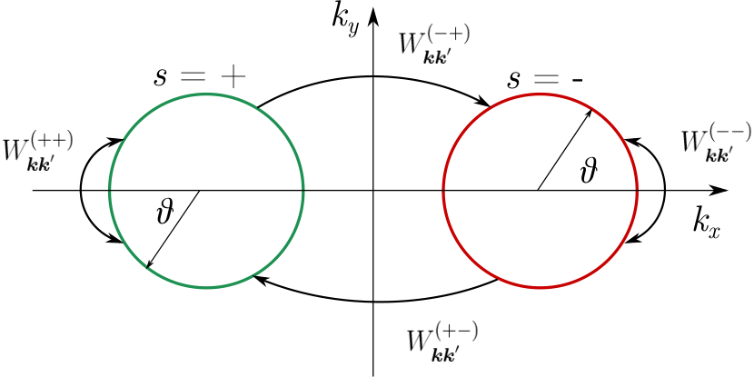
In this subsection, we demonstrate the effect of inter-valley scattering on the current induced valley density difference $\Delta n_{0}$ by solving the semi-classical Boltzmann equation (SBE). We simplify the Fermi surface at each valley as a circular Fermi pocket as shown in Fig. 4, and will argue later that this simplification doesn’t change the result qualitatively. The calculation is carried out in the absence of interactions, i.e. in the paramagnetic phase, so that time reversal symmetry is present, which imposes $\epsilon^{s}(\bm{k})=\epsilon^{\bar{s}}(-\bm{k})$ and $\bm{v}^{s}(\bm{k})=-\bm{v}^{\bar{s}}(-\bm{k})$, where $s=\pm$ is the valley index with $s\neq\bar{s}$. No other point group symmetries are assumed.

The SBE within the presence of a bias electric field $\bm{E}$ is given byKamenev 2011; Lifshitz and Pitaevskii 1981:

The measure in the collision integral is defined as $\mathop{}\!\mathrm{d}\Gamma^{\prime}=\frac{d^{2}k^{\prime}}{(2\pi)^{2}}$. Both the intra-valley scattering, $W^{(++)}_{\bm{k}\bm{k}^{\prime}}$ and $W^{(--)}_{\bm{k}\bm{k}^{\prime}}$, as well as the inter-valley ones, $W^{(-+)}_{\bm{k}\bm{k}^{\prime}}$ and $W^{(+-)}_{\bm{k}\bm{k}^{\prime}}$, are included. TRS requires that $W^{(++)}_{\bm{k}\bm{k}^{\prime}}=W^{(--)}_{\bm{k}^{\prime}\bm{k}}$ and $W^{(-+)}_{\bm{k}\bm{k}^{\prime}}=W^{(+-)}_{\bm{k}^{\prime}\bm{k}}$. Here, we assume detailed balance, which follows from the first Born approximation.

We look for a static solution of the SBE, Eq. (6), within linear response. The distribution function can be conveniently parameterized by harmonic coefficients:

where $f_{0}$ is the equilibrium Fermi distribution function, the angle $\theta_{\bm{k}}$ is defined for each valley as shown in Fig. 4. The harmonic coefficients, $x^{(s)}_{n}$ and $y^{(s)}_{n}$, are proportional to $\bm{E}$ within linear response. The valley density difference is determined by:

where $\nu$ is the density of states at the Fermi level. Notice that the simplification to the second line of Eq. (8) is a result of the assumed circular Fermi pockets, see Fig. 4.

Before presenting the solution of the Boltzmann equation, we point out the central role of inter-valley scattering. Namely, to obtain non-zero valley density difference, $\Delta n_{0}$, the inter-valley scattering rate must be treated with care. In particular, a constant inter-valley scattering rate $1/\tau^{\prime}$ cannot generate a nonzero valley density difference in the static limit. To see this point, one can integrate the SBE, Eq. (6), over the full Brillouin zone, assuming that the inter-valley scattering rate is a constant, $W^{\text{inter}}$. The result is a continuity equation for the valley densities: $\partial_{t}n^{(\pm)}-\nabla\cdot\bm{j}^{(\pm)}=-\left(n^{(\pm)}-n^{(\mp)}\right)/\tau^{\prime}$, where the inter-valley scattering time is defined as $\tau^{\prime-1}=\nu W^{\text{inter}}$. In a spatially uniform and time independent system, the right hand side must vanish, which indicates that the valley density difference always relaxes and vanishes in the static limit, even though we allowed for non-zero (but constant) inter-valley scattering. To avoid this problem, one must account for momentum-dependent inter-valley scattering, which will induce a “source” in the continuity equation.

Following the reasoning above, we consider the inter-valley scattering rate given by:

which explicitly breaks rotational symmetry. The dimensionless parameters $a_{1}^{\vphantom{\prime}},a_{1}^{\prime}$ and $b_{1}^{\vphantom{\prime}},b_{1}^{\prime}$ are determined by the microscopic mechanisms of breaking rotational symmetry.

For demonstration purposes, we make two additional simplifications. First, we assume the intra-valley scattering is constant,

where $\nu$ and $\tau$ are the density of states and the intra-valley scattering time, respectively. Second, the Fermi surfaces are assumed to be circular. Indeed, given the inter-valley scattering rate in Eq. (9), the detailed form of the intra-valley scattering and the Fermi surface geometry are expected to play a secondary role on the generation of valley polarization. They do not affect whether a valley density difference can be generated by external bias or not. They only affect the magnitude of the valley density difference, at a similar level to other microscopic details that are beyond our model calculations.

The solution to Eq. (6) is physically intuitive in the limit that the intra-valley scattering time ($\tau$) is much shorter than the inter-valley one ($\tau^{\prime}$). To leading order in $\tau/\tau^{\prime}$, the static solution satisfies the SBE with only the intra-valley scattering,

The harmonic expansion coefficients of the distribution function are

where $\tau$ is the intra-valley scattering time, $v_{\text{F}}$ is the Fermi velocity defined from $\bm{v}_{\bm{k}_{F}}^{(s)}=s\,v_{\text{F}}(\cos\theta_{\bm{k}},\sin\theta_{\bm{k}})$. Note that without inter-valley scattering, there is no constraint on $x^{(s)}_{0}$ from the SBE because the number density of each valley is separately conserved.

Now the static valley density difference can be determined by solving $0=I_{\text{inter}}^{(s)}[f_{\bm{k}}]$:

This equation dictates a balance between the inter-valley relaxation process (the first two terms) and a “source” (the last term in parentheses) that generates the valley density difference. The “source” originates from the interplay between the nonequilibrium distribution function from Eq. (12) and the rotational symmetry breaking of the inter-valley scattering rate, Eq. (9).

Solving Eq. (13), we find that the valley density difference $\Delta n_{0}=n^{\scriptscriptstyle(+)}-n^{\scriptscriptstyle(-)}$ is given by:

or, equivalently expressed in terms of the current density $\bm{j}=\sigma\bm{E}$:

Notice the bulk longitudinal conductivity $\sigma$ is related to the intra-valley scattering rate $\tau$ through $\sigma=2\frac{e^{2}}{h}h\nu D$, where $D=\frac{1}{2}v_{\text{F}}^{2}\tau$ is the two dimensional diffusion constant and the prefactor of $2$ accounts for the two valleys.

The simplified model presented in this subsection can be solved exactly. The valley density difference for a general ratio of inter- and intra-valley scattering time, $\tau^{\prime}/\tau$, is shown in Fig. 5. Indeed, when the inter-valley scattering time is much longer than the intra-valley one, the valley density difference saturates to a value given by Eq. (15). On the other hand, $\Delta n_{0}$ decreases with decreasing inter-valley scattering time. $\Delta n_{0}$ vanishes when the inter-valley relaxation time $\tau^{\prime}$ goes to zero.

As has been emphasized, inter-valley scattering is essential to obtain a current induced valley density difference, because it is the channel to exchange electrons between the two valleys. Without inter-valley scattering, the electron density within each valley is exactly conserved.

The valley density difference in Eq. (15) is determined by the first harmonic of the inter-valley scattering rate, which explicitly breaks the discrete rotational symmetry of the system to $\mathcal{C}_{1z}$. In the next section, we determine the coefficients $a_{1},a^{\prime}_{1},b_{1},b^{\prime}_{1}$ in Eq. (9) from microscopic modeling of h-BN aligned TBG with $\mathcal{C}_{1z}$ symmetry.

Finally, the valley density difference is proportional to the current, Eq. (15), as we restricted ourselves to linear response. By reversing the current direction, the valley density difference is also reversed, and hence so is the valley polarization, see Eq. (4). Therefore, we conclude that with broken rotational symmetry, the valley polarization can be controlled by a DC current.

In this subsection, we estimate the valley density difference for the TBG/h-BN system. As has been emphasized, to induce $\Delta n_{0}\neq 0$ from a bias electric field, the lattice rotational symmetry needs to be fully broken. While unaligned TBG exhibits the higher symmetry point group $D_{3}$, a close alignment of either top or bottom TBG layer with h-BN not only breaks the sublattice (inversion) symmetry, but also can induce strain to the sample that further breaks $\mathcal{C}_{3z}$ to $\mathcal{C}_{1z}$. In the following, we model the rotational symmetry breaking by strain.

A full account of the microscopic details of magic angle TBG to obtain the valley density difference is quite challenging, and requires the full knowledge of the inter-valley scattering mechanism as well as the spectrum and wavefunctions of TBG near the magic twist angle. Nevertheless, the mechanism we proposed in Sec. III.1 is generic. The magnitude of the effect, parametrized by the coefficient $\bm{\delta}_{\epsilon}$ in the valley density difference Eq. (5), is a reflection of the degree of rotational symmetry breaking. For example, in strained single layer graphene, $\bm{\delta}_{\epsilon}\sim\epsilon$, where $\epsilon$ is the strain strength. In this sense, a general mechanism that enhances the effect of strain would be desirable to explain the small critical current observed in the experiment. In the following, we show that in TBG aligned with h-BN, due to the interplay between two comparable lengths – the moiré scale ($a/\theta_{w}$) and the strain scale ($a/\epsilon$) – the strain effect is enhanced to $\epsilon\rightarrow\frac{\epsilon}{\theta_{w}}$. To demonstrate this point, it is enough to introduce the inter-layer tunneling perturbatively, which preserves the analytical solubility.

Our modeling is based on the continuous model, introduced in Ref. Bistritzer and MacDonald 2011 and generalized in Ref. Balents 2019 that captures elastic deformations systematically. Here, we assume a uniaxial strain parameterized by the strain tensorHe et al. 2020

where $\epsilon$ is a dimensionless parameter characterizing the strain strength. $\nu_{\epsilon}=0.165$ is the Poisson ratio for graphene. $\phi$ is the direction of the strain. Note that only the first term in Eq. (16) breaks rotational symmetry and enters into $\bm{\delta}_{\epsilon}$.

Without loss of generality, we consider the strain only on layer 1, Fig. 6. Due to the combination of the strain field and the alignment with the h-BN substrate, the Dirac Hamiltonian around the K-point becomes $H=v_{\text{D}}\bm{k}\cdot(1+\bm{\mathcal{E}})\cdot\bm{\sigma}+m\sigma_{z}$Balents 2019, where $v_{\text{D}}$, $\bm{k}$ and $m$ are the Dirac velocity, the momentum measured from the Dirac point and the mass gap, respectively. At the leading order in the strain strength, the rotational symmetry breaking of the continuous model under the strain field is reflected in several aspects. First, the Dirac points at $K^{(\prime)}$ valleys are shifted by $\delta{\bm{K}}^{(\prime)}_{i}=-\underline{\bm{\mathcal{E}}}\cdot{\bm{K}}^{(\prime)}_{i}$ for the strained layerBalents 2019. As a result, the momentum difference between the adjacent Dirac points of the two layers, see Fig. 3, is modified as

where ${\bm{q}}_{i}=\theta_{w}{\bm{K}}_{i}\times\hat{z}$, $i\in\{1,2,3\}$. Second, the single layer hopping integral is modified due to the strain field, which modifies the single layer energetics and shift the Dirac points also at order $\epsilon/a$. Third, the Dirac spectrum is anisotropic. However, the Dirac spectrum anisotropy is parametrically smaller in $|{\bm{k}}|/|{\bm{K}}|$ than the shift of the Dirac point, Balents 2019 and is thus neglected.

For simplicity, only the first contribution is included in the following discussions. As the wave vectors for inter-layer tunneling ${\bm{q}}^{\prime}_{i}-{\bm{q}}^{\prime}_{1}$, i.e. the the reciprocal lattice vector of the moiré Brillouin zone (mBZ), are modified due to the strain, the $\mathcal{C}_{3}$ rotational symmetry of the mBZ is broken explicitly [see Fig. 3(b)], and the effect is characterized by:

where both the shift of the Dirac point under strain field, $\delta\bm{K}\sim\epsilon\left|\bm{K}\right|$, and the size of mBZ, $q=\theta_{w}\left|\bm{K}\right|$, are small and comparable to each other.

We focus on bulk transport. From the discussion of Sec. III.1, both intra- and inter-valley scattering of TBG must be taken into account properly. The dominant scattering mechanism in TBG is yet to be determined, but certain key features may be captured by simple modeling. Here, we consider short range impurities and a low doping level (well below $3/4$ filling of the moiré conduction band) so that there is a Fermi pocket around each Dirac point at the corner of the mBZ (see Fig. 6). Notice that the inter-valley scattering involves a much larger momentum transfer than the intra-valley one. Therefore, we assume the intra-valley scattering time $\tau$ being much shorter than the inter-valley scattering time $\tau^{\prime}$, which is expected to be generically true for most scattering mechanisms in TBG.

As discussed in the previous subsection, the intra-valley scattering only plays a secondary role in the generation of valley density difference by a bias DC current. Hence, we assume the intra-valley scattering is dominated by the scattering within each Fermi pocket with a constant relaxation time, $\tau$. The inter-valley scattering requires more careful examination to obtain the coefficients $a_{1},a^{\prime}_{1},b_{1},b^{\prime}_{1}$ in Eq. (9). There are several processes as shown in Fig. 6. With simple on-site disorder, it turns out that the scattering between the two valleys in the same graphene layer does not break $\mathcal{C}_{3z}$ and generate non-zero $a_{1},a^{\prime}_{1},b_{1},b^{\prime}_{1}$ since we neglected the anisotropy of the Dirac spectrum. Thus, the scattering rates between the two valleys of the same graphene layer are taken to be constant, $\left(\nu\tau^{\prime}\right)^{-1}$, as indicated by the green arrows in Fig. 6. At the same time, the scattering rates between the two valleys in different layers may break rotational symmetry through the process indicated by the red arrows in Fig. 6. It is directly related to the shift of the Dirac points due to strain as well as the coherent inter-layer tunneling. As in Fig. 6, the scattering rates of such processes are of order $\sim\left(\nu\tau^{\prime}\right)^{-1}t^{2}$, where $t$ is a dimensionless perturbation parameter for the inter-layer tunneling, Eq. (86).

After fitting the scattering rates into the semi-classical Boltzmann equation introduced in the previous subsection, we obtain the valley density difference generated by a DC current. The main result is summarized in Fig. 7, where, without loss of generality, only one graphene layer is strained (see Appendix B for more details of the calculation).

When the strain strength is zero, $\mathcal{C}_{3z}$ is restored and the valley density difference is identically zero. For non-zero strain strength, the valley density difference appears as expected from the breaking of $\mathcal{C}_{3}$ symmetry. At small strain strength, the valley density difference is linear in the strain strength:

where the basic scale for current induced density is $n_{{\bm{j}}}=\frac{3t^{2}/4}{1+3t^{2}/4}\frac{1}{hv_{F}}\frac{h}{e^{2}}ej$. Here $\theta_{{\bm{j}}}$ is the angle of the current, $\phi$ is the angle of uniaxial strain as defined in Eq. (16). The small numerical value in Fig. 7 is a result of the low doping assumption, where $v_{\text{D}}k_{\text{F}}/m$ is a small parameter with $k_{\text{F}}$ being the Fermi momentum. The result is further suppressed by the inter-layer tunneling $t^{2}$, which is assumed to be small to introduce the inter-layer tunneling perturbatively.

Even though our result, Fig. 7 and Eq. (19), was obtained with a set of very specific assumptions (weak inter-layer coupling and low doping level), some implications can be drawn for real samples. In reality, there are several comparable scale: moiré band width, inter-layer coupling and the mass gapBistritzer and MacDonald 2011; Kim et al. 2018. Therefore, the dimensionless parameter $t^{2}$ is not small. In addition, the phenomenon of current switching of valley polarization is observed at three quarter filling. Thus, it is reasonable to expect that the small factor of $v_{\text{D}}k_{\text{F}}/m$ in Eq. (19) is lifted and is on the order of $\mathcal{O}(1)$. Therefore, we conclude that the actual valley density difference can be estimated as:

with a numerical coefficient on the order of $\mathcal{O}(1)$. Based on the arguments above, one may roughly estimate that a small DC current ($\sim 10^{-3}\text{A}/\text{m}$) could generate a large valley density difference on the order of $10^{11}\text{m}^{-2}$. This is comparable to the effect of magnetic field ($\sim\nu\mu_{\text{B}}B$ and $B\sim 10\ \text{mT}$ with $\mu_{\text{B}}$ being the Bohr magneton)Serlin et al. 2020.

References

- Serlin et al. (2020) M. Serlin, C. Tschirhart, H. Polshyn, Y. Zhang, J. Zhu, K. Watanabe, T. Taniguchi, L. Balents, and A. Young, Science 367, 900 (2020).
- Sharpe et al. (2019) A. L. Sharpe, E. J. Fox, A. W. Barnard, J. Finney, K. Watanabe, T. Taniguchi, M. Kastner, and D. Goldhaber-Gordon, Science 365, 605 (2019).
- Stoner (1938) E. C. Stoner, Proceedings of the Royal Society of London. Series A. Mathematical and Physical Sciences 165, 372 (1938).
- Sondhi et al. (1993) S. L. Sondhi, A. Karlhede, S. A. Kivelson, and E. H. Rezayi, Phys. Rev. B 47, 16419 (1993).
- MacDonald et al. (1996) A. H. MacDonald, H. A. Fertig, and L. Brey, Phys. Rev. Lett. 76, 2153 (1996).
- Cao et al. (2018a) Y. Cao, V. Fatemi, A. Demir, S. Fang, S. L. Tomarken, J. Y. Luo, J. D. Sanchez-Yamagishi, K. Watanabe, T. Taniguchi, E. Kaxiras, et al., Nature 556, 80 (2018a).
- Cao et al. (2018b) Y. Cao, V. Fatemi, S. Fang, K. Watanabe, T. Taniguchi, E. Kaxiras, and P. Jarillo-Herrero, Nature 556, 43 (2018b).
- Dodaro et al. (2018) J. F. Dodaro, S. A. Kivelson, Y. Schattner, X. Q. Sun, and C. Wang, Phys. Rev. B 98, 075154 (2018).
- Zou et al. (2018) L. Zou, H. C. Po, A. Vishwanath, and T. Senthil, Phys. Rev. B 98, 085435 (2018).
- Zhang et al. (2019a) Y.-H. Zhang, D. Mao, Y. Cao, P. Jarillo-Herrero, and T. Senthil, Phys. Rev. B 99, 075127 (2019a).
- Balents et al. (2020) L. Balents, C. R. Dean, D. K. Efetov, and A. F. Young, Nature Physics , 1 (2020).
- Po et al. (2018a) H. C. Po, H. Watanabe, and A. Vishwanath, Phys. Rev. Lett. 121, 126402 (2018a).
- Zhang et al. (2019b) Y.-H. Zhang, D. Mao, and T. Senthil, Phys. Rev. Research 1, 033126 (2019b).
- Isobe et al. (2018) H. Isobe, N. F. Q. Yuan, and L. Fu, Phys. Rev. X 8, 041041 (2018).
- Nandkishore et al. (2012) R. Nandkishore, L. Levitov, and A. Chubukov, Nature Physics 8, 158 (2012).
- Chichinadze et al. (2020a) D. V. Chichinadze, L. Classen, and A. V. Chubukov, Phys. Rev. B 101, 224513 (2020a).
- Chichinadze et al. (2020b) D. V. Chichinadze, L. Classen, and A. V. Chubukov, Phys. Rev. B 102, 125120 (2020b).
- Xu and Balents (2018) C. Xu and L. Balents, Phys. Rev. Lett. 121, 087001 (2018).
- Po et al. (2018b) H. C. Po, L. Zou, A. Vishwanath, and T. Senthil, Phys. Rev. X 8, 031089 (2018b).
- Yankowitz et al. (2019) M. Yankowitz, S. Chen, H. Polshyn, Y. Zhang, K. Watanabe, T. Taniguchi, D. Graf, A. F. Young, and C. R. Dean, Science 363, 1059 (2019).
- Lu et al. (2019) X. Lu, P. Stepanov, W. Yang, M. Xie, M. A. Aamir, I. Das, C. Urgell, K. Watanabe, T. Taniguchi, G. Zhang, A. Bachtold, A. H. MacDonald, and D. K. Efetov, Nature 574, 653 (2019).
- Cao et al. (2020) Y. Cao, D. Rodan-Legrain, J. M. Park, F. Noah Yuan, K. Watanabe, T. Taniguchi, R. M. Fernandes, L. Fu, and P. Jarillo-Herrero, arXiv e-prints , arXiv:2004.04148 (2020), arXiv:2004.04148 [cond-mat.mes-hall] .
- Jiang et al. (2019) Y. Jiang, X. Lai, K. Watanabe, T. Taniguchi, K. Haule, J. Mao, and E. Y. Andrei, Nature 573, 91 (2019).
- Hejazi et al. (2019a) K. Hejazi, C. Liu, H. Shapourian, X. Chen, and L. Balents, Phys. Rev. B 99, 035111 (2019a).
- Hejazi et al. (2019b) K. Hejazi, C. Liu, and L. Balents, Phys. Rev. B 100, 035115 (2019b).
- Saito et al. (2020) Y. Saito, J. Ge, K. Watanabe, T. Taniguchi, and A. F. Young, Nature Physics 16, 926 (2020).
- Xie et al. (2019) Y. Xie, B. Lian, B. Jäck, X. Liu, C.-L. Chiu, K. Watanabe, T. Taniguchi, B. A. Bernevig, and A. Yazdani, Nature 572, 101 (2019).
- Tschirhart et al. (2020) C. L. Tschirhart, M. Serlin, H. Polshyn, A. Shragai, Z. Xia, J. Zhu, Y. Zhang, K. Watanabe, T. Taniguchi, M. E. Huber, and A. F. Young, arXiv e-prints , arXiv:2006.08053 (2020), arXiv:2006.08053 [cond-mat.mes-hall] .
- Kang and Vafek (2019) J. Kang and O. Vafek, Phys. Rev. Lett. 122, 246401 (2019).
- Polshyn et al. (2020) H. Polshyn, J. Zhu, M. A. Kumar, Y. Zhang, F. Yang, C. L. Tschirhart, M. Serlin, K. Watanabe, T. Taniguchi, A. H. MacDonald, and A. F. Young, Nature 588, 66 (2020).
- Bultinck et al. (2020) N. Bultinck, S. Chatterjee, and M. P. Zaletel, Phys. Rev. Lett. 124, 166601 (2020).
- Ochi et al. (2018) M. Ochi, M. Koshino, and K. Kuroki, Phys. Rev. B 98, 081102 (2018).
- Chang and Niu (2008) M.-C. Chang and Q. Niu, Journal of Physics: Condensed Matter 20, 193202 (2008).
- Xiao et al. (2010) D. Xiao, M.-C. Chang, and Q. Niu, Rev. Mod. Phys. 82, 1959 (2010).
- He et al. (2020) W.-Y. He, D. Goldhaber-Gordon, and K. T. Law, Nature Comm. 11, 1 (2020).
- Huang et al. (2020) C. Huang, N. Wei, and A. MacDoanld, arXiv e-prints , arXiv:2007.05990 (2020), arXiv:2007.05990 [cond-mat.mes-hall] .
- Kamenev (2011) A. Kamenev, Field theory of non-equilibrium systems (Cambridge University Press, 2011).
- Altland and Simons (2010) A. Altland and B. D. Simons, Condensed matter field theory (Cambridge university press, 2010).
- Mermin (1967) N. D. Mermin, Journal of Mathematical Physics 8, 1061 (1967).
- Lifshitz and Pitaevskii (1981) E. Lifshitz and L. P. Pitaevskii, Physical Kinetics, Volume 10 (Course of Theoretical Physics) (Pergamon Press, New York, 1981).
- Bistritzer and MacDonald (2011) R. Bistritzer and A. H. MacDonald, Proceedings of the National Academy of Sciences 108, 12233 (2011).
- Balents (2019) L. Balents, SciPost Phys 7, 48 (2019).
- Kim et al. (2018) H. Kim, N. Leconte, B. L. Chittari, K. Watanabe, T. Taniguchi, A. H. MacDonald, J. Jung, and S. Jung, Nano Lett. 18, 7732 (2018).
Appendix A Valley Polarization Order Parameter Dynamics from Keldysh Formalism
This section is for the demonstration of the valley polarization in the twisted bilayer graphene (tBLG) with the presence of an external bias. The ‘slow’ dynamics of the valley polarization order parameter, denoted by and its Fourier transformation , is governed by the following action: