Kernel optimization for Low-Rank Multi-Fidelity Algorithms

We describe the core idea behind low-rank MF methods, as outlined in [28]. The construction of $\tilde{g}_{H}$ proceeds in two steps. In the first step, the parameter space $D$ is explored via the low-fidelity model to identify “important” points in parameter space. Since by assumption $g_{L}$ is an inexpensive emulator, this is practically feasible. The procedure for accomplishing this exploration is essentially numerical linear algebra.

First we densely sample $D$ with the ensemble $\{p_{j}\}_{j=1}^{N}$, where $N\gg 1$. These points may be selected in any reasonable way: as Monte Carlo samples, equispaced samples, low-discrepancy samples, etc. We next construct a Gramian matrix $G_{L}$ with entries:

$\displaystyle(G_{L})_{l,j}$

$\displaystyle=K\left(g_{L}(p_{l}),g_{L}(p_{j})\right),$

$\displaystyle l,j$

$\displaystyle=1,\ldots,N,$

$\displaystyle K(u,v)$

$\displaystyle=\left\langle u,v\right\rangle,$

(1)

where $\langle\cdot,\cdot\rangle$ is the standard Euclidean inner product on $\mathbb{R}^{m}$. This Gramian is positive semi-definite, but is not definite if $N<m$. In this case, the first $m$ steps of a pivoted Cholesky decomposition can be completed:

$\displaystyle PG_{L}P^{T}=LL^{T},$

(2)

where $L$ is a lower-triangular matrix and is zero for rows $m+1,\ldots,N$. The permutation matrix $P\in\mathbb{R}^{N\times N}$ determines an “important” point selection, in particular, the vector

$\displaystyle z\coloneqq P\left(\begin{array}[]{c}1\\ 2\\ \vdots\\ N\end{array}\right),$

is used to define an ordering $p_{z_{1}},p_{z_{2}},\ldots,p_{z_{N}}$ of the $N$ parameter points. For any $n\leq m$, the point set

$\displaystyle\widehat{D}=\left\{p_{z_{1}},\ldots,p_{z_{n}}\right\}\subset D$

(3)

are the “important” points. For later purposes we will also require an $n\times n$ matrix $\widehat{G}_{L}$, which is a $z$-sliced version of $G_{L}$:

$\displaystyle\left(\widehat{G}_{L}\right)_{i,j}$

$\displaystyle=\left(G_{L}\right)_{z_{i},z_{j}},$

$\displaystyle i,j$

$\displaystyle=1,\ldots,n.$

The identification of $\widehat{D}$ is the main purpose of the first step. The second step will require evaluations of the HF model on $\widehat{D}$, so that $n$ is usually chosen based on the available computational budget.

This approach for selecting “important” points via pivots is computationally efficient [43, 36] and is equivalent to the pivoted samples selected by a column-pivoted QR decomposition of a matrix of model realizations [28]. Pivots from an LU factorization are also used in the area of computational fluid dynamics and heat transfer [2] similarly. Alternative statistical strategies such as leverage-score sampling methods [33] and group matching methods [26, 32] are also useful for the selection of optimal/important set of sampling points. For the purposes of simplicity in this paper, we focus exclusively on the Cholesky approach for identifying points. The second step of the MF procedure first computes the HF ensemble,

$\displaystyle\left\{g_{H}(p_{z_{i}})\right\}_{i=1}^{n},$

which is feasible if $n$ is small. The MF approximation is built as a linear expansion over this ensemble:

$\displaystyle g_{H}(p)\approx\widetilde{g}_{H}(p)\coloneqq\sum_{l=1}^{n}g_{H}\left(p_{z_{l}}\right)c_{l}(p),$

(4)

where $\{c_{l}(p)\}_{l=1}^{n}$ are coefficients in a vector $c(p)$ that is computed via a least-squares projection on the low-fidelity model:

$\displaystyle\widehat{G}_{L}c(p)=\left(\begin{array}[]{c}K\left(g_{L}(p),g_{L}(p_{z_{1}})\right)\\ \vdots\\ K\left(g_{L}(p),g_{L}(p_{z_{n}})\right)\end{array}\right).$

Note that the right-hand side of the above equation is computable immediately simply by evaluating the $g_{L}(p)$, i.e., the low-fidelity model. The least squares projection coefficients can be obtained as

$\displaystyle c(p)=\widehat{G}_{L}^{-1}\left(\begin{array}[]{c}K\left(g_{L}(p),g_{L}(p_{z_{1}})\right)\\ \vdots\\ K\left(g_{L}(p),g_{L}(p_{z_{n}})\right)\end{array}\right).$

Note in particular that the emulator is interpolatory on the trained samples $\{p_{i}\}_{i=1}^{n}$, i.e., $g_{H}(p_{i})=\widetilde{g}_{H}(p_{i})$ for all $i=1,\ldots,n$. This property can be directly deduced by noting in (2.1) that if $p=p_{z_{i}}$, then the right-hand side is exactly a column of $\widehat{G}_{L}$, and so all the $c_{j}(p_{i})$ coefficients vanish, except for $c_{j}(p_{j})=1$. This procedure can be generalized to include more levels of fidelity [28, 43], which is advantageous when three or more models exist.

In summary, the first stage of the algorithm is “offline”, which requires the computation of $N\gg 1$ realizations of the LF model. Some (inexpensive) linear algebra identifies a small set of $n\ll N$ parameter values where the HF model is evaluated in step 2. Then for each fixed $p\in D$, the low-rank MF surrogate in (4) is computed by first evaluating $g_{L}(p)$, and then by solving (2.1) for the vector $c(p)$.

While the MF surrogate $\widetilde{g}_{H}$ certainly achieves the cost requirement (evaluation requires only low-fidelity effort), understanding its accuracy is more subtle. The authors in [28] provide abstract error certification in general Hilbert spaces; however the analysis is not useful in practice and the bound derived is not computable. In [22] a more practical analysis demonstrates that this surrogate is accurate when the LF and HF models correspond time integration solvers with coarse and fine timesteps, respectively. Finally, the authors in [18] provide a statistical strategy for computationally certifying error committed by $\widetilde{g}_{H}$.

Assuming $\widetilde{g}_{H}$ is accurate, the major limitations of this approach are described in Section 1. We give a more detailed discussion here. First recall that since $G_{L}$ has rank $m$ at most, then when $m\ll N$ only the first $n=m$ pivots selected in the decomposition (2) are informative. (The remaining $N-m$ pivots are essentially selected at random due to floating-point roundoff errors.) To see why this can become an issue, consider $g_{L}$ as a scalar output of a model (for example, the section lift coefficient in an aerodynamics model). Then the MF procedure only produces a single informative parameter value. This prevents the procedure from taking advantage of additional HF model runs when such runs are computationally feasible.

A second limitation is in the stability of the linear solver required in (2.1). When $G_{L}$ is a low-rank matrix, then its singular values decay quickly, and the sliced matrix $\widehat{G}_{L}$ is ill-conditioned. This can numerically pollute the MF surrogate (4).

A final limitation that we will discuss is more subtle: one requirement for success of this procedure is that $G_{L}$ is “similar” to $G_{H}$, where $G_{H}$ is a HF Gramian defined similarly as (1) but with $g_{H}$ instead of $g_{L}$. The choice of $K$ in (1) to take uncentered inner products may not reveal similarity of $G_{L}$ and $G_{H}$, but choosing a different function $K$ may improve this approximation.

In this section, let $i$ be a fixed family index associated to one of the kernel families in Table 1. Our task is to determine an appropriate value of the hyperparameter $h$. We formulate this selection as a simple optimization problem, where we impose that the following requirements should be met:

• •

  To maintain accuracy, the optimized kernel should behave like the linear kernel $K_{1}$ (since when the Gramian $G_{L}$ is well-conditioned, results in the literature [28, 22] show that this procedure is effective).

• •

  To maintain stability, the Gramian $G_{L}$ resulting from a particular choice of kernel should reasonably be well-conditioned.

Our desire to maintain accuracy of the MF emulator is not always aligned with ensuring that a selected kernel behaves like the linear kernel. However, the current success of the linear kernel in the literature suggests that this may promote some accuracy[35, 36, 28]. In addition, the main purpose of the accuracy requirement is to ensure that the chosen hyperparameters do not force the kernel function to concentrate to a Dirac delta function: if the kernel focuses to the Dirac delta function, then the MF approximation will suffer poor accuracy. The choice of proximity to the linear kernel is thus just one choice of regularizer; we implement this as the Frobenius norm proximity to the linear kernel Gramian.

The need to maintain stability comes from the fact that solving (2.1) should be numerically stable. When the Gramian matrix is rank-deficient, the stability consideration regularizes the matrix so that its rank deficiency is mitigated. We implement this as the numerical (or stable) rank of the Gramian.

In summary, with $i\geq 2$ fixed, let $G_{L}^{i}(h)$ denote $N\times N$ the low-fidelity Gramian matrix associated with using $K=K_{i}(h)$ in (1). I.e., $G_{L}^{i}(h)$ has entries

$\displaystyle\left(G_{L}^{i}(h)\right)_{j,k}=K_{i}(u_{L}(p_{j}),u_{(}p_{k});h).$

We choose a value for the hyperparameters $h$ via the optimization problem

$\displaystyle h^{\ast}=\argmin_{h}f_{\text{obj}}(h)\coloneqq\left\|G^{1}_{L}-G_{L}^{i}(h)\right\rVert_{F}+\lambda\frac{1}{\sqrt{\mathrm{srank}\left(G_{L}^{i}(h)\right)}}$

(14)

where $\lambda$ is tunable parameter, $\|\cdot\|_{F}$ is the Frobenius norm on matrices, and $\mathrm{srank}(\cdot)$ is the numerical/stable rank:

$\displaystyle\mathrm{srank}(A)=\frac{\|A\|^{2}_{F}}{\|A\|^{2}_{2}}.$

The objective function $f_{\textrm{obj}}$ in (14) thus seeks to simultaneously promote proximity to the linear Gramian (“accuracy”) and maximization of the numerical rank (“stability”). The value of $\lambda$ can be obtained by empirical testing. In practice we judge that this procedure finds an effective kernel if $h^{\ast}\sim\lambda/\sqrt{n}$, corresponding to a case when the error in the adaptive kernel Gramian balances with the numerical rank. However, we expect optimal values of this parameter to be problem-dependent. For all problems tested in this paper, we found that $\lambda=0.1$ provided good results, obtained through grid search and evaluating by computing errors on testing data. This value of $\lambda$ was computed using a logarithmic grid search over the first three test problems in this manuscript. Using this approach, $\lambda$ is a regularization parameter that promotes the numerical stability of the solution, and the grid search we have employed is one of the standard approaches in machine learning [6, 23] for tuning such a regularization parameter.

As often the number of hyperparameters is small (cf. Table 1) and the computational cost of high-fidelity model evaluation is significantly higher than that of the low-fidelity model, the process of hyperparameter optimization is inexpensive in contrast. Note that the optimization (14) operates only on the low-fidelity model, and the objective function is simple and efficient to evaluate if all the low-fidelity data is stored.

In order to deal with this problem, we propose two approaches that generalizes the kernel function selection framework. For both of these proposed approaches we are using a heuristic optimization algorithm called particle swarm algorithm [21, 11] to minimize $f_{\text{obj}}$ in Eq. 14. Next, this algorithm is briefly discussed.

The optimization problem (14) has $\dim h$ design variables, and for our choices of kernels this number is relatively small (see Table 1). Nevertheless, gradient-based optimization algorithms can perform poorly when the initial guess is far away from a basin of attraction. To mitigate this issue, we employ particle swarm optimization [21, 11] to compute a reasonable initial guess, and subsequently perform a gradient-based interior point algorithm.

Particles swarm optimization (PSO) is a velocity-based evolutionary optimization approach, and was initially developed for modeling social behaviors in bird flocks using topological neighborhoods [12]. PSO is initialized using an ensemble of random points in the design/search space, with each ensemble member called a particle. For each particle there is an assigned position (design variable value) and velocity. The initial selection of particle positions and velocities is often random from a uniform distribution. The remaining portion of the algorithm updates particle positions and velocities using a notion of fitness of a particle, i.e., an estimate of its optimality relative to the ensemble.

Let $\{h_{i}\}_{i=1}^{S}$ and $\{v_{i}\}_{i=1}^{S}$ be the position and velocity, respectively, of the $i$th particle. For $n\in\mathbb{N}$, let $h_{i}^{n}$ denote the position of the $i$th particle at PSO iteration $n$. At $n=1$, all positions and velocities are randomly initialized. PSO updates proceed by:

	$\displaystyle v^{n+1}_{i}$	$\displaystyle=$	$\displaystyle v^{n}_{i}+k_{1}\rho\left(B^{n}_{i}-h^{n}_{i}\right)+k_{2}\gamma\left(B^{n}_{g}-h^{n}_{i}\right),$		(15)
	$\displaystyle h^{n+1}_{i}$	$\displaystyle=$	$\displaystyle h^{n}_{i}+v^{n+1}_{i},$

where $B^{n}_{i}$ and $B^{n}_{g}$ denote the best solution for the $i$th particle in iterations $1,...,n$, and group’s best solution for iterations $1,\ldots,n$, respectively. I.e.,

$\displaystyle B_{i}^{n}$

$\displaystyle\coloneqq\min_{j\in[n]}f_{\text{obj}}(h_{i}^{j}),$

$\displaystyle B_{g}^{n}$

$\displaystyle\coloneqq\min_{(i,j)\in[S]\times[n]}f_{\textrm{obj}}(h_{i}^{j}),$

$\displaystyle[n]$

$\displaystyle\coloneqq\{1,2,\ldots n\}.$

The parameters $\rho$ and $\gamma$ in (15) are uniform random variables on $[0,1]$ (independent at each time and for each particle) and $k_{1}$ and $k_{2}$ are tunable parameters. We apply standard velocity clamping procedures to ensure velocities remain bounded and particles do not leave the design space: If some particle’s velocity exceeds a maximum allowed velocity limit, it is set to the maximum allowed value of velocity [38]. PSO iterations continue until a stopping criterion is triggered. In our case, we limit the maximum number of iterations and lack of improvement in the group’s best solution. There are many variations of PSO; for the purpose of this study we employ the MATLAB toolbox “particleswarm solver”. This algorithm has been shown to be faster than standard evolutionary algorithms in approaching the vicinity of the minima [5, 4].

However, PSO is slow when it comes to converging to a local minimum once a basin of attraction is reached. Therefore, we use loose criteria to terminate the PSO iterations, and subsequently use the best particle as the initial guess into a gradient-based interior point algorithm (with finite difference approximated gradient); the output of the gradient-based algorithm is our computed value of $h^{\ast}$ in (14).

We have discussed in Sections 3.1 and 3.2 how we select the hyperparameter value $h$ for each kernel index $i$ in Table 1. This section and the following section propose two strategies for choosing an overall kernel $K$ for use in the MF procedure of Section 2.1.

Our first approach, the Additive Kernel Approach, choose an overall kernel $K$ as an additive mixture of all kernels in the library:

$\displaystyle K(u,v)$

$\displaystyle=\sum_{i=1}^{L}w_{i}K_{i}(u,v;h_{i}^{\ast}),$

$\displaystyle(w_{1},\ldots w_{L})$

$\displaystyle\in\{x\in\mathbb{R}^{L}\;\big|\;\sum_{\ell=1}^{L}x_{\ell}=1,\;\;x_{\ell}\in[0,1]\;\;\forall i\}$

(16)

where $L$, $h^{\ast}_{i}$ and $w_{i}$ are the number of kernel functions in the library ($L=7$ in this paper), the $i$th optimized hyperparameter value $h^{\ast}$ output from (14), and its corresponding weight. The optimizations associated with computing the quantities in (16) are convex, so several types of algorithms are appropriate. We again employ PSO for an initial guess, followed by an interior-point algorithm for accelerated convergence to a minimum.

The full MF procedure is exactly as described in Section 2.1, with $K$ in (1) the kernel computed in (16). We emphasize again that the choice of kernel only depends on low-fidelity data. Only after a kernel function is chosen do we query the HF model through the procedure in Section 2.1.

Our second procedure for selecting a kernel is the Adaptive Kernel Approach. In this procedure, we select only one kernel $K_{i}$ as the kernel of choice in the MF procedure. However, the index of this choice $i$ depends on the HF simulation budget $n$. In brief, with $n$ fixed, we select $i$ as the kernel index that results in the best approximation of a size-$n$ least squares approximation of the LF model.

In detail, we first fix $i$ and construct $\widetilde{g}_{L,i}$ as an emulator for the LF model using kernel $i$:

$\displaystyle\widetilde{g}_{L}(p)=\sum_{l=1}^{n}g_{L}\left(p_{z_{l,i}}\right)c_{l,i}(p),$

(17)

where $\{z_{l,i}\}_{l=1}^{n}$ are the pivots selected from the Cholesky decomposition of $G_{L}$ in (1) with $K=K(\cdot,\cdot;h^{\ast}_{i})$. The coefficients $\{c_{l,i}\}_{l=1}^{n}$ are entries in the least-squares coefficient vector $c_{i}(p)$ from a linear system similar to (2.1):

$\displaystyle\widehat{G}_{L}c_{i}(p)=\left(\begin{array}[]{c}K\left(g_{L}(p),g_{L}(p_{z_{1,i}})\right)\\ \vdots\\ K\left(g_{L}(p),g_{L}(p_{z_{n,i}})\right)\end{array}\right),$

where again $K=K(\cdot,\cdot;h^{\ast}_{i})$. The function $\widetilde{g}_{L}$ is an emulator for $g_{L}$ built via a least squares approximation. One error metric for this least squares emulator is

$\displaystyle\epsilon_{i}\coloneqq\textrm{med}_{j\in[N]\backslash\{z_{1,i},\ldots,z_{n,i}\}}\left\|g_{L}(p_{j})-\widetilde{g}_{L}(p_{j})\right\|,$

where med denotes the median. Note that the error $\left\|g_{L}(p_{j})-\widetilde{g}_{L}(p_{j})\right\|=0$ when $j\in\{p_{z_{1,i}},\ldots,p_{z_{n,i}}\}$ represents the indices of the training samples. The median has been chosen as the summary statistic for the distribution of the residuals for multi-fidelity emulators since the errors do not necessarily follow a normal (or symmetric) distribution and it is most often skewed. Moreover, the median is an effective statistic for summarizing distributions [13] and thus provides a more robust measure of error for our purpose. We emphasize that the data used to train the emulator is the set of parameters $\{p_{z_{i}}\}_{i=1}^{n}$. In this testing phase we compute errors over the set of realizations corresponding to the parameters $\{z_{i}\}_{i=1}^{N}\backslash\{p_{z_{i}}\}_{i=1}^{n}$ that the emulator was not trained with.

To choose the “best” kernel index $i^{\ast}$, we choose

$\displaystyle i^{\ast}=\argmin_{i=1,\ldots,n}\epsilon_{i}.$

Finally, we choose $K$ in (1) as $K=K_{i^{\ast}}(h^{\ast})$. Like the Additive kernel approach, this approach analyzes only the LF model, and hence is computationally feasible. However, this approaches differs from the additive approach in that the optimal $i^{\ast}$ is recomputed when $n$ is changed.

The classical computational algorithm for performing molecular dynamics (MD) simulations has been developed based upon the Lagrangian methodology of tracking particle dynamics via Newton’s equations of motion. Numerical integration of these equations provides an accurate evaluation of the time evolution of a molecular system, and hence the system’s quantities of interest. While there are many integration schemes available in the literature, but we settle on the velocity Verlet algorithm [25] due to its popularity, reasonable accuracy, and simplicity of implementation. The Lennard-Jones (LJ) potential was used for simulating the interatomic interactions in the MD system. The potential function also has parameters $\epsilon$, the potential well depth, and $\sigma$, the length scale for the pairwise interatomic interaction.

In the process of MD simulation using any interatomic interaction model, when the size of the integration time-step is large, the major challenge is the stability of the MD integration scheme. If the time-step is too large, then iterations may predict near-collocation of molecules/atoms which will lead to large (unphysical) repulsive forces and large displacements on the next time step, and this instability snowballs to future time steps. To prevent such divergence of the integration scheme, we clamp the magnitude of repulsive interactions for closely-approaching atoms. For our LJ potential, this capping can be implemented straightforwardly by modifying the potential at short distance.

The MF situation we consider here are models whose fidelity is defined by the choice of integration time step. The parameters $p\in\mathbb{R}^{2}$ we consider are the temperature and the density of the molecular system. For every parameter value, quantities of interest are computed using the low-fidelity model (here, the MD simulation with a large time-step $\Delta t$) and concatenated into an output vector. The quantities of interest we consider here are the scalar averaged total energy $E$ and diffusion coefficient $D$:

$$g(p_{j})=\left[\frac{E(p_{j})}{\sqrt{\overline{E}}},\frac{D(p_{j})}{\sqrt{\overline{D}}}\right]^{T}.$$

(24)

We have rescaled the parameters by their averaged values over the ensemble:

	$\displaystyle\overline{E}$	$\displaystyle=$	$\displaystyle\frac{1}{N}\sum_{j=1}^{N}\|E(p_{j})\|_{2}^{2},$
	$\displaystyle\overline{D}$	$\displaystyle=$	$\displaystyle\frac{1}{N}\sum_{j=1}^{N}\|D(p_{j})\|_{2}^{2}.$		(25)

Note that in MD simulations there are other important quantities of interest, such as the radial distribution function (RDF) and mean squared displacement (MSD). For this test problem, we consider a uniform grid of temperature and density defined as $T\times\rho:[500,1000]\text{K}\times[36.27,701.29]\frac{\text{kg}}{\text{m}^{3}}$ ($\rho^{\ast}:[0.05,0.95]$) with $N=114$ sample points, where $\rho$ and $\rho^{\ast}$ are density and dimensionless density equal to $\frac{Nm}{V}$ and $\frac{N\sigma^{3}}{V}$, respectively. We also assume $\sigma$, $\varepsilon$, $m$ or molecular mass to be $3\textup{\AA}$, $1\frac{\text{kcal}}{\text{mol}}$ and 12.01$\frac{\text{g}}{\text{mol}}$, respectively. Here, the boundary conditions in all sides of cubic simulation box (with the width of 27.05Å) are considered to be periodic. Here the mass of each particle ($m$) and simulation box size ($L=V^{\frac{1}{3}}$) is set to 12.01 g/mol and 27.05Å, respectively.

The LF model is defined by an MD simulation with time step $\Delta t=20$fs, and the HF model is the same MD simulation with $\Delta t=1$fs. In this situation, the dimension of the vector $g_{L}(p)$ is 2, and hence the naive MF procedure in Section 2.1 with the linear kernel can only take $n=2$ meaningful HF samples. Figure 1 demonstrates that the Additive/Adaptive kernel approaches circumvent this limitation. We see that the linear kernel error stagnates since after $n=2$ the “important” parameter values are chosen essentially randomly, and furthermore the least squares problem (2.1) becomes ill-conditioned. However, both the Additive and Adaptive kernel approaches produce more reasonable errors, with improvements gained as one is able to invest more HF effort.

As shown in Fig 1 (a) and (c), both proposed approaches work well although the error is not monotonically decreasing with respect to increased effort. This lack of monotonic error is due to the fact that we use kernel evaluations of the low-fidelity model on the right-hand side of (2.1) in the place of the (unavailable) high-fidelity kernel evaluation. In panes (b) and (d) we show the error of the RDF and MSD quantities of interest for this procedure, which were not used in formation of the MF surrogate. Thus, this procedure does not overfit energy and diffusion at the cost of other quantities.

Another reason for the non-monotonic reduction of the error with respect to the increase in effective high fidelity simulation is variable computational costs of molecular simulation, which are directly proportional to molecular density or the number of particles in the simulation box. Hence, addition of one high-fidelity sample does not linearly increase the cumulative computational cost.

Here, both proposed approaches outperform the naive multi-fidelity method that applies the linear kernel function. The rank deficiency of the constructed Gramian matrix for the linear kernel approach is the main reason for such poor performance. This ill-conditioned Gramian matrix itself results from the low dimension of the model output space for low- and high-fidelity models.

Additionally, the results illustrated in Fig 1 indicate about two orders of magnitude in error reduction when the effective number of high-fidelity simulation increase from 8 to 14. This is supporting evidence for the success of the proposed multi-fidelity kernel optimization approach in handling a difficult predictive task for a complex system with underlying stochastic behavior.

Next, we consider a more difficult MD simulation with a two-component glass-forming system. In this case, the three output parameters of both LF and HF models are the diffusion coefficients $D_{A}$ and $D_{B}$ for species A and B, along with the total energy $E$.

We perform output normalization similar to (25). Here, the length scale for pairwise interatomic interactions between molecules are set as $\sigma_{A}=3.5\textup{\AA}$ for interactions between molecules of species A, $\sigma_{B}=3.888\textup{\AA}$ for B-B interactions, and $\sigma_{AB}=\sqrt{\sigma_{A}\sigma_{B}}$ for A-B interactions interaction between both types of molecules. For this experiment, we have $N=24$ points in the density-temperature (parameter) space. The number of molecules in the MD simulation for each species is 512. Once again, the boundary conditions are assumed to be periodic for all sides of the simulation box. The temperature and simulation box length for these sample points vary between 180K and 290K, and 37.62Å and 38.35Å, respectively. Once again, the results depicted in Fig. 2 shows high accuracy of both adaptive and additive models for prediction of the three radial distribution functions involving interactions of molecules of type A and B ($R_{AA}$, $R_{AB}$ and $R_{BB}$) as well as the corresponding diffusion coefficients and system total energy. However these results indicate that, if performing 12 high-fidelity simulation is computationally affordable, the multi-fidelity model constructed based on the proposed adaptive kernel function selection approach is slightly more accurate compared to the one constructed using the additive approach and significantly more accurate when compared to the multi-fidelity solution with linear kernel function.

Furthermore, as the number of particles is fixed for each sample, a more monotonic trend of convergence can be observed for this case (see Fig. 2). Due to the smaller number of training low-fidelity data points, the accuracy of the approach degrades. On the other hand, while radial distribution functions are not involved in the construction of the multi-fidelity models, the accuracy of the emulator for their estimation is quite good: around 1 percent error with only 1/3 of the high-fidelity samples.

Galaxy systems often can be modeled as an $n$-body problem, in which the gravitational dynamics governs the interaction between objects. The interaction force between the objects can be driven from Newton’s law of gravity as [41]

$$F_{i}=-\sum_{\begin{subarray}{c}j=1\\ j\neq i\end{subarray}}^{n}{\frac{Gm_{i}m_{j}\left(r_{i}-r_{j}\right)}{|r_{i}-r_{j}|^{3}}},$$

(26)

where $G$, $m_{i}$ and $r_{i}$ are the gravitational constant, $i$th object mass, and distance of $i$th object from the origin, respectively. Considering a cutoff radius can simplify the calculation, as the force between each object and any other object outside this radius is automatically set to zero. For the purpose of this study, the GalaxSee $n$-body model [19] is used as the simulation module.

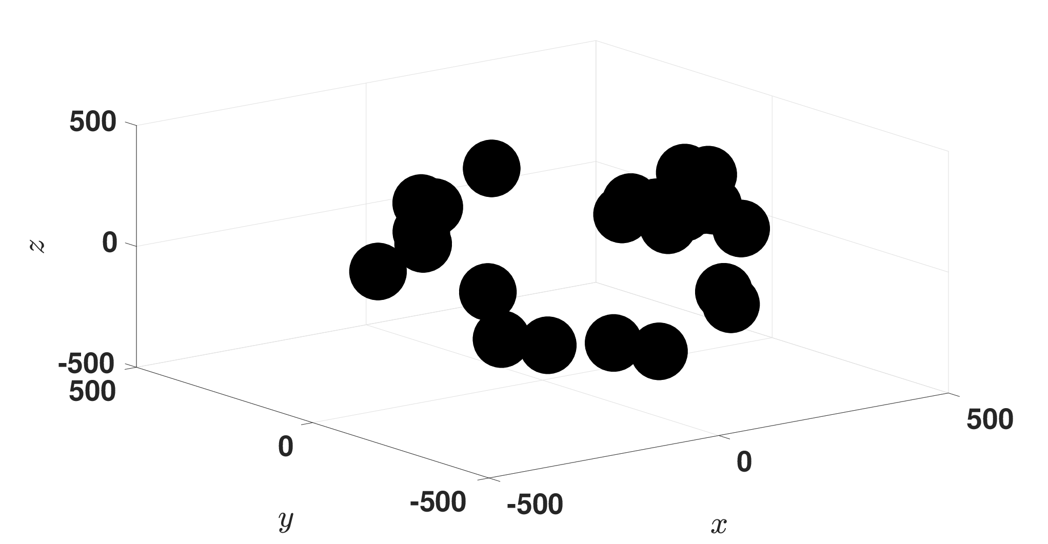
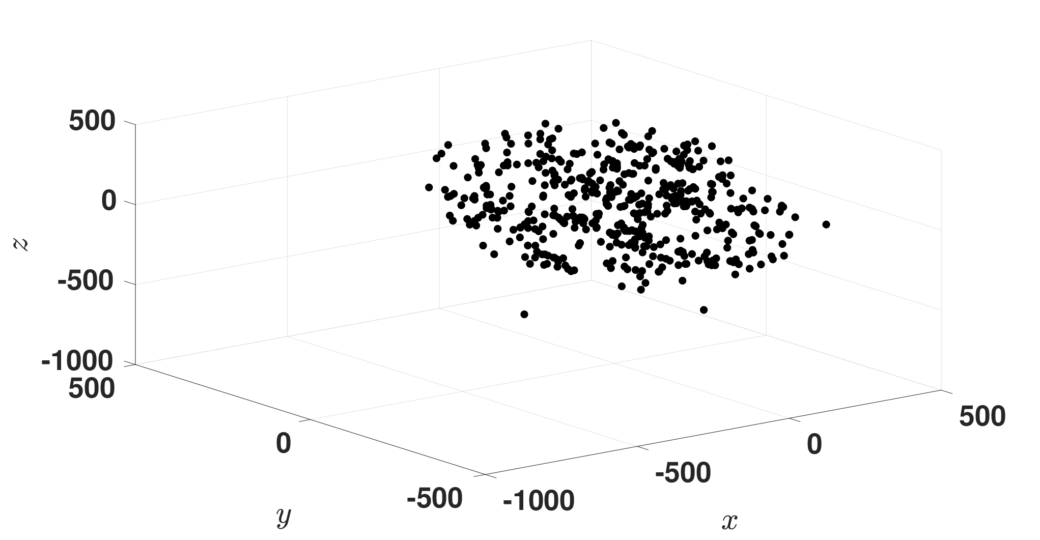
The parameter space for this case involve system’s total mass ($M\in[50,500]$ solar mass) and the initial rotation ($\Gamma\in[0,0.9]$) about a central axis in the $n$-body cluster imposed on the system. Fidelity here is based on quantized parameters in the model [35]: We consider galaxy systems of 25 and 500 objects as the low- and high-fidelity models, respectively. The quantities of interest for this test problem are total energy, mean distance from the origin, and the mean velocity of the objects in galaxy systems. As illustrated in Fig. 3, the evolutions of both low- and high-fidelity models is significantly different, and thus we do not expect to be able to use MF simulations to compute detailed trajectories; however, our quantities of interest are averaged metrics, and so using a MF surrogate procedure can be effective. The results provided in Fig. 4 indicate success of of the kernel selection procedures for constructing MF emulators. This level of accuracy is obtained despite the apparent failure of the standard linear kernel MF surrogate. Thus, the kernel selection procedure takes advantages of the optimization process to promote numerical stability and accuracy. Here, the Adaptive Kernel Approach provides us with a slightly more accurate predictive model. This could be the result excluding several “improper” choices of kernel function. In the Additive Kernel Approach for this problem, every kernel function in the library has a non-zero contribution in construction of the additive kernel.

As shown in Fig. 4, the cost of multi-fidelity simulations scales proportionally to the cost of each added high-fidelity simulation sample. By increasing the number of high-fidelity samples from 4 to 18 for the construction of the multi-fidelity emulator, the prediction error of the emulator models reduces by around two orders of magnitude. This is the case for all outputs of the model, and for two of the proposed approaches. This level of accuracy is achieved despite the complexity of the dynamical system, but is possible by considering only averaged characteristics of the system. We expect significant decline of accuracy if particle trajectories or velocities are directly predicted.

Telechelic associated polymer networks in their equilibrium condition can be modeled as a Simulated Gel Network (SGN) with its nodes characterized as “peers” and “superpeers”; for details see [7]. The number of links and nodes in the network depends on the temperature. For this test problem, the fractions of superpeers ($n_{s}$) and peers ($n_{p}$) at non-dimensional temperature ($T$) of 0.55 based on the Table 1 of Ref. [7] are set to be 0.604 and 0.396, respectively. The following system of equations and constraints model the network that exhibits the same properties as those of an SGN:

	$\displaystyle n_{s}\langle k\rangle_{s}$	$\displaystyle=$	$\displaystyle 2l_{ss}+l_{ps},$
	$\displaystyle n_{p}\langle k\rangle_{s}$	$\displaystyle=$	$\displaystyle l_{ps}+2l_{pp},$
	$\displaystyle l_{\text{tot}}$	$\displaystyle=$	$\displaystyle l_{pp}+l_{ps}+l_{ss},$
	$\displaystyle l{ss}$	$\displaystyle=$	$\displaystyle(0.85\pm 0.01)l_{\text{tot}},$
	$\displaystyle l{pp}$	$\displaystyle=$	$\displaystyle(0.02\pm 0.01)l_{\text{tot}},$
	$\displaystyle l{ps}$	$\displaystyle=$	$\displaystyle(0.13\pm 0.01)l_{\text{tot}},$		(27)

where, $l_{ss}$, $l_{ps}$, and $l_{pp}$ represent the probability of having a connection between two superpeers, between one peer and a superpeer, and between two peers, respectively. Here $\langle k\rangle$ denotes the average degree (number of connections for each node), and for $T=0.55$ is set to be $\langle k\rangle=7.131$ and $\langle k\rangle=0.997$ for superpeers and peers, respectively. We consider 1200 nodes for the model network and randomly generate links based on the calculated values of $l_{ss}$, $l_{ps}$, and $l_{pp}$.

In order to study the topological change in the simulated associating polymers under constant stress, we consider the following governing equations for the nodal strain evolution in the network [9]:

$$\frac{d\varepsilon}{dt}=\frac{1}{\eta}A\sigma_{0},$$

(28)

where $\eta$, $\sigma_{0}$, $\varepsilon$ and $A$ are a coefficient of viscosity, vectors of constant stress, time-dependent strain and the network’s adjacency matrix, respectively. For this test problem, we consider the of effective resistances between any two nodes in a network and use a graph sparsification process [40] to obtain a low-fidelity network model. Hence, the high- and low-fidelity models in this case are fully dense and sparsified networks, respectively. Here, the parameter space is obtained by uniform random variation of the viscosity coefficient and constant in $[0.05,2.5]$ and between 0 and 2.5, respectively. Two scalar quantities of interest for this test problem are the mean and standard deviation of the resulting strain field at $t=10$. In this case the output quantities of interest are two-dimensional vectors. Once again, as shown in Fig. 5, the dimension of the outputs being small directly impacts the accuracy of the standard (linear kernel) multi-fidelity model. However, the MF models using the new modified kernel approaches perform much better. Similar to the result of the previous test problems, the adaptive approach appears to be more cost-effective and results in a more accurate predictive model. Once again, this better accuracy is the result of selection of the optimal kernel function exclusively in the adaptive approach instead of estimation of the contribution factor for each kernel function in the function library in the additive approach.

Here, as the number of nodes in both low- and high-fidelity networks are the same, the computational cost of the simulation for both are roughly the same. This is the main reason behind the large number of effective high-fidelity simulations required to obtain a reasonable level of accuracy for the MF emulators.

In a wide range of real-world technical problems in engineering, the quantities of interest are scalar quantities. As mentioned previously in this paper, using the linear kernel function in such a situation is essentially ineffective, producing an MF emulator with only 1 degree of freedom, and results in a surrogate model with a significant inaccuracy. Designing a plasmonic nano-particle array with an optimal scattering and/or extinction efficiency is among these real-world scenarios. For the calculation of these efficiency parameters as well as simulation of the optical response of a set of identical non-magnetic metallic nano-spheres with sizes much smaller than the wavelength of light (here 25 nm) the Coupled Dipole Approximation (CDA) method [17] is used. Using this method, for $N$ metallic nano-particles described by the same volumetric polarizability $\alpha(\omega)$ and located at vector positions $r_{i}$, one can compute the local field $E_{loc}(r_{i})$ as:

$$\left(1-\frac{\alpha k^{2}}{\epsilon_{0}}\sum_{j=1,j\neq i}^{N}\mathbf{\tilde{G}}_{ij}\right)\mathbf{E}_{loc}(\mathbf{r}_{i})=\mathbf{E}_{0}{\mathbf{r}_{i}},$$

(29)

where $\mathbf{E}_{0}(r_{i})$ is the incident field in vector form, $k$ is the wavenumber in the background medium, $\epsilon_{0}$ is the dielectric permittivity of vacuum ( $\epsilon_{0}=1$ in CGS unit system), and $\mathbf{\tilde{G}}_{ij}$ is constructed from $3\times 3$ block of the overall $3N\times 3N$ Green’s matrix for the $i$th and $j$th particles and the summation runs through all $j$th particles except for $j=i$.

By solving (29), the total local fields ($\mathbf{E}_{loc}(r_{i})$) are computed, and consequently the local electric dipole polarizations across the array can be determined. The scattering and extinction cross-sections can be computed using the resulting polarizations. Finally, the corresponding extinction ($Q_{ext}$) and scattering ($Q_{sc}$) efficiencies are obtained by normalization of scattering and extinction cross-sections with respect to the total projected area of the array (i.e., sum of the areas of the particles projected perpendicularly to the direction of the excitation beam).

In particular we consider Vogel spirals arrays [10, 37], which can uniquely identify useful nano-particle array configurations with only four parameters: the number of particles, ($\alpha_{vs}$), divergence angle, incident wavelength, and scaling factor.

Here, the number of particles in the array defines the level of fidelity. Varying this fidelity parameter can result in significantly different outputs (compare the two panels in each of Figs. 6 and Figs. 7). Also the limited dimension of the output parameter space for this case makes the choice of the linear kernel function prohibitive. The results shown in Figs. 8 and 9 confirm this deduction for MF models of silver and aluminum nano-particle arrays. The number $N$ of particles in the low- and high-fidelity models for both cases are $N=25$ and $N=100$, respectively for Figure 6, and are $N=50$ and $N=1000$ for Figure 7, respectively. Both of the novel kernel selection approaches are successfully applied to develop surrogate models with much higher accuracy (see Figs. 8 and 9). The computational cost of the kernel selection optimization for this test problem are insignificant in comparison to the cost of running one high-fidelity simulation. Hence, the prediction error of the multi-fidelity emulator coverages more smoothly and monotonically. Here, the accuracy of both new kernel selection MF methods appear to be similar.

Due to the complexity of plasmonic models for large-scale arrays of particles, the prediction accuracy is lower in Figs. 6 compared to Figs. 7. Another reason for this lower accuracy is the more pronounced difference between parametric dependence of the low- and high-fidelity nanoparticle arrays and corresponding plasmonic models. Similar parametric dependence between low- and high-fidelity models is beneficial for the selection of a better set of high-fidelity sampling points.

Our previous examples have investigated the two proposed kernel selection schemes when the model output space has small dimension. In most of the cases above, the adaptive kernel approach has a small advantage. However, it is also necessary to investigate the performance of these approaches for cases in which the dimension of output space is high enough to pick sufficient number of “important” samples for the construction of the MF model even with the linear kernel function. The objective of considering this test problem is to provide some insights about the competitiveness of the adaptive kernel approach compared to the linear kernel function method, when the Gramian matrix for both is not ill-conditioned. Since the previous examples suggest that the adaptive kernel procedure is slightly more accurate than the additive method, we focus on highlighting results for the adaptive kernel only. Note that the additive kernel is slightly less computationally expensive than the adaptive kernel method.

In many fluid dynamics problems a large amount of data can be extracted from a solution, and thus are a good example of high-dimensional output space. Here, we consider a two-dimensional incompressible stenotic flow in a large channel with a length and width of 11$m$ and 1 $m$, respectively. The shape of the curve of stenosis in the middle of the channel follows the equation (see Fig 10):

$$y(x,y_{0})=1-\frac{y_{0}}{2}\left(1+\cos{\left(2\pi\left(x-5\right)\right)}\right).$$

(30)

The parameter space for this problem is two-dimensional, comprised of the flow Reynolds number (Re) and the parameter $y_{0}$: $(\text{Re},y_{0})\in[0.1,0.6]\times[10,500]$. The inlet flow stream has a velocity of 1$m/s$ and for simplicity the fluid kinematic viscosity $\nu$ is set to be $1/\text{Re}$. The goal of constructing predictive models for this problem is to estimate horizontal and vertical velocity ($u$ and $v$, respectively) profiles in the middle of the channel ($x=5.5$m) as well as the shear stress on top and bottom wall of the channel ($y=0$ and 1, respectively) at $t=30$ sec. The HF model in this case solves the full unsteady incompressible Navier-Stokes equation, which can be written in vector form as follows [3]:

$$\frac{\partial U}{\partial t}+\frac{\partial E}{\partial x}+\frac{\partial F}{\partial y}+H=0,$$

(31)

where

	$\displaystyle U$	$\displaystyle=$	$\displaystyle[0,u,v]^{T},$
	$\displaystyle E$	$\displaystyle=$	$\displaystyle[u,u^{2}+P-\nu\frac{\partial u}{\partial x},uv-\nu\frac{\partial v}{\partial x}]^{T},$
	$\displaystyle F$	$\displaystyle=$	$\displaystyle[v,uv-\nu\frac{\partial u}{\partial y},v^{2}+P-\nu\frac{\partial v}{\partial y}]^{T},$
	$\displaystyle H$	$\displaystyle=$	$\displaystyle[-f_{x},-f_{y},-f_{z}]^{T}.$

Here, $P$ and $f$ denote pressure and external force, respectively. The LF model is the coupled linearized Navier-Stokes equation, which are obtained by decomposing the solution into a basic state and perturbed state:

$$\frac{\partial V}{\partial t}+W\cdot\nabla{V}+V\cdot\nabla{W}=-\nabla{P}+\nu\nabla^{2}{V}+f,$$

(32)

where $W$ and $W+\varepsilon V$ are the basic and perturbed states, respectively and $\varepsilon<<1$.

Both Eqs. (31) and (32) can be cast into a the form of $L(U)=B$ for a linear operator $L$ and $U$-independent term $B$. Via a Galerkin discretization, this can subsequently be cast in matrix form:

$$A\hat{U}=\hat{B},$$

(33)

where

	$\displaystyle\hat{B}_{m}$	$\displaystyle=$	$\displaystyle\int_{\Omega}{\Phi_{m}Bdx},$
	$\displaystyle A_{m,n}$	$\displaystyle=$	$\displaystyle\int_{\Omega}{\Phi_{m}L\left(\Phi_{n}\right)Bdx},$

where $\Phi_{m}$ are basis functions for the Galerkin method. We solve this problem using Nektar++, which is an open-source spectral/hp element software [8]. Fourth order polynomials are used to approximate the finite element solution of the problem. Both low- and high-fidelity models use the same mesh but they are different with respect to their corresponding solution models, and as shown in Fig. 11 this difference leads to a significant difference in the prediction of the flow field in the channel at $t=30$ sec. The accuracy of the quantities of interest obtained from low-rank MF models with respect to the effective number of high-fidelity model evaluations is illustrated in Fig. 12. In this figure, the adaptive kernel MF method produces accuracy comparable to the linear kernel MF method for all quantities of interest. Figure 13 provides a clear picture for the inaccuracy of the low-fidelity model and the resulting enhancement in the predictions of the MF models. These results indicate that there is no penalty for considering a more complex kernel selection procedure in this example. Since the more complex kernel selection procedure does perform better than the linear kernel method for other examples, this suggests that using the adaptive kernel approach rather than the linear kernel approach is a better choice in general.

References

- [1] D. Allaire and K. Willcox, A mathematical and computational framework for multifidelity design and analysis with computer models, International Journal for Uncertainty Quantification, 4 (2014).
- [2] D. Anderson and M. Gu, An efficient, sparsity-preserving, online algorithm for low-rank approximation, in International Conference on Machine Learning, 2017, pp. 156–165.
- [3] D. Anderson, J. C. Tannehill, and R. H. Pletcher, Computational fluid mechanics and heat transfer, CRC Press, 2016.
- [4] P. J. Angeline, Evolutionary optimization versus particle swarm optimization: Philosophy and performance differences, in International Conference on Evolutionary Programming, Springer, 1998, pp. 601–610.
- [5] , Using selection to improve particle swarm optimization, in Evolutionary Computation Proceedings, 1998. IEEE World Congress on Computational Intelligence., The 1998 IEEE International Conference on, IEEE, 1998, pp. 84–89.
- [6] J. Bergstra and Y. Bengio, Random search for hyper-parameter optimization, The Journal of Machine Learning Research, 13 (2012), pp. 281–305.
- [7] J. Billen, M. Wilson, A. Rabinovitch, and A. R. Baljon, Topological changes at the gel transition of a reversible polymeric network, EPL (Europhysics Letters), 87 (2009), p. 68003.
- [8] C. D. Cantwell, D. Moxey, A. Comerford, A. Bolis, G. Rocco, G. Mengaldo, D. De Grazia, S. Yakovlev, J.-E. Lombard, D. Ekelschot, et al., Nektar++: An open-source spectral/hp element framework, Computer Physics Communications, 192 (2015), pp. 205–219.
- [9] R. Christensen, Theory of viscoelasticity: an introduction, Academic Press, 1982.
- [10] A. C. Christofi, F. A. Pinheiro, and L. Dal Negro, Probing scattering resonances of Vogel’s spirals with the Green’s matrix spectral method, Optics Letters, 41 (2016), pp. 1933–1936.
- [11] M. Clerc, Particle swarm optimization, vol. 93, John Wiley & Sons, 2010.
- [12] S. Deepa and G. Sugumaran, Model order formulation of a multivariable discrete system using a modified particle swarm optimization approach, Swarm and Evolutionary Computation, 1 (2011), pp. 204–212.
- [13] I. Dittmann and E. G. Maug, Biases and error measures: How to compare valuation methods, ERIM Report Series Reference No. ERS-2006-011-F&A, (2008), pp. 2006–07.
- [14] G. F. Fasshauer, Meshfree Approximation Methods With Matlab, World Scientific Publishing Company, Singapore ; Hackensack, N.J, Apr. 2007.
- [15] M. G. Fernández-Godino, C. Park, N.-H. Kim, and R. T. Haftka, Review of multi-fidelity models, arXiv:1609.07196 [stat], (2016). arXiv: 1609.07196.
- [16] M. B. Giles, Multilevel Monte Carlo methods, Acta Numerica, 24 (2015), pp. 259–328.
- [17] C.-A. Guérin, P. Mallet, and A. Sentenac, Effective-medium theory for finite-size aggregates, Journal of the Optical Society of America A, 23 (2006), pp. 349–358.
- [18] J. Hampton, H. R. Fairbanks, A. Narayan, and A. Doostan, Practical error bounds for a non-intrusive bi-fidelity approach to parametric/stochastic model reduction, Journal of Computational Physics, 368 (2018), pp. 315–332.
- [19] P. Jacobs, P. List, M. Ludin, A. Weeden, and R. M. Panoff, The blue waters student internship program: promoting competence and confidence for next generation researchers in high-performance computing, in Proceedings of the Workshop on Education for High-Performance Computing, IEEE Press, 2014, pp. 49–55.
- [20] L. Jofre, G. Geraci, H. Fairbanks, A. Doostan, and G. Iaccarino, Multi-fidelity uncertainty quantification of irradiated particle-laden turbulence, arXiv preprint arXiv:1801.06062, (2018).
- [21] J. Kennedy, Particle swarm optimization, in Encyclopedia of machine learning, Springer, 2011, pp. 760–766.
- [22] V. Keshavarzzadeh, R. Kirby, and A. Narayan, Convergence Acceleration for Time-Dependent Parametric Multifidelity Models, SIAM Journal on Numerical Analysis, 57 (2019), pp. 1344–1368. arXiv: 1808.03379.
- [23] A. Klein, S. Falkner, S. Bartels, P. Hennig, and F. Hutter, Fast bayesian optimization of machine learning hyperparameters on large datasets, in Artificial Intelligence and Statistics, 2017, pp. 528–536.
- [24] R. Lam, D. L. Allaire, and K. E. Willcox, Multifidelity optimization using statistical surrogate modeling for non-hierarchical information sources, in 56th AIAA/ASCE/AHS/ASC Structures, Structural Dynamics, and Materials Conference, 2015, p. 0143.
- [25] J. G. Lee, Computational materials science: an introduction, CRC press, 2016.
- [26] A. Lozano, G. Swirszcz, and N. Abe, Group orthogonal matching pursuit for logistic regression, in Proceedings of the Fourteenth International Conference on Artificial Intelligence and Statistics, 2011, pp. 452–460.
- [27] A. Mehmani, S. Chowdhury, C. Meinrenken, and A. Messac, Concurrent surrogate model selection (COSMOS): optimizing model type, kernel function, and hyper-parameters, Structural and Multidisciplinary Optimization, 57 (2018), pp. 1093–1114.
- [28] A. Narayan, C. Gittelson, and D. Xiu, A stochastic collocation algorithm with multifidelity models, SIAM Journal on Scientific Computing, 36 (2014), pp. A495–A521.
- [29] B. Peherstorfer, K. Willcox, and M. Gunzburger, Survey of multifidelity methods in uncertainty propagation, inference, and optimization, SIAM Review, 60 (2018), pp. 550–591.
- [30] P. Perdikaris, D. Venturi, and G. E. Karniadakis, Multifidelity information fusion algorithms for high-dimensional systems and massive data sets, SIAM Journal on Scientific Computing, 38 (2016), pp. B521–B538.
- [31] P. Perdikaris, D. Venturi, J. Royset, and G. Karniadakis, Multi-fidelity modelling via recursive co-kriging and Gaussian–Markov random fields, Proc. R. Soc. A, 471 (2015), p. 20150018.
- [32] D. Perry, R. Kirby, A. Narayan, and R. Whitaker, Allocation Strategies for High Fidelity Models in the Multifidelity Regime, SIAM/ASA Journal on Uncertainty Quantification, 7 (2019), pp. 203–231. arXiv: 1812.11601 [math.NA].
- [33] D. J. Perry and R. T. Whitaker, Augmented leverage score sampling with bounds, in Joint European Conference on Machine Learning and Knowledge Discovery in Databases, Springer, 2016, pp. 543–558.
- [34] C. E. Rasmussen, Gaussian Processes in Machine Learning, in Advanced Lectures on Machine Learning, Lecture Notes in Computer Science, Springer, Berlin, Heidelberg, 2004, pp. 63–71.
- [35] M. Razi, A. Narayan, and R. M. Kirby, Fast predictive multi-fidelity prediction with models of quantized fidelity levels, Journal of Computational Physics, 376 (2019), pp. 992–1008.
- [36] M. Razi, A. Narayan, R. M. Kirby, and D. Bedrov, Fast predictive models based on multi-fidelity sampling of properties in molecular dynamics simulations, Computational Material Science, 152 (2018), pp. 125–133.
- [37] M. Razi, R. Wang, Y. He, R. M. Kirby, and L. Dal Negro, Optimization of large-scale Vogel spiral arrays of plasmonic nanoparticles, Plasmonics, (2018).
- [38] F. Shahzad, A. R. Baig, S. Masood, M. Kamran, and N. Naveed, Opposition-based particle swarm optimization with velocity clamping (ovcpso), in Advances in Computational Intelligence, Springer, 2009, pp. 339–348.
- [39] R. Skinner, A. Doostan, E. Peters, J. Evans, and K. E. Jansen, An evaluation of bi-fidelity modeling efficiency on a general family of NACA airfoils, in 35th AIAA Applied Aerodynamics Conference, 2017, p. 3260.
- [40] D. A. Spielman and N. Srivastava, Graph sparsification by effective resistances, SIAM Journal on Computing, 40 (2011), pp. 1913–1926.
- [41] M. Trenti and P. Hut, Gravitational N-body simulations, arXiv preprint arXiv:0806.3950, (2008).
- [42] X. Zhu, E. M. Linebarger, and D. Xiu, Multi-fidelity stochastic collocation method for computation of statistical moments, Journal of Computational Physics, 341 (2017), pp. 386–396.
- [43] X. Zhu, A. Narayan, and D. Xiu, Computational aspects of stochastic collocation with multifidelity models, SIAM/ASA Journal on Uncertainty Quantification, 2 (2014), pp. 444–463.