A quantum double in a superconducting wire array
Abstract
We show that a quantum double can be realized in an array of superconducting wires coupled via Josephson junctions. With a suitably chosen magnetic flux threading the system, the inter-wire Josephson couplings take the form of a complex Hadamard matrix, which possesses combinatorial gauge symmetry — a local symmetry involving permutations and shifts by of the superconducting phases. The sign of the star potential resulting from the Josephson energy is inverted in this physical realization, leading to a massive degeneracy in the non-zero flux sectors. A dimerization pattern encoded in the capacitances of the array lifts up these degeneracies, resulting in a topologically ordered state. Moreover, this dimerization pattern leads to a larger effective vison gap as compared to the canonical case with the usual (uninverted) star term. We further show that our model maps to a quantum three-state Potts model under a duality transformation. We argue, using a combination of bosonization and mean field theory, that altering the dimerization pattern of the capacitances leads to a transition from the topological phase into a quantum XY-ordered phase. Our work highlights that combinatorial gauge symmetry can serve as a design principle to build quantum double models using systems with realistic interactions.
I Introduction
The identification of possible experimental realizations of topologically ordered states of matter remains a central problem in condensed matter physics. The fractional quantum Hall (FQH) effects Tsui et al. 1982; Laughlin 1983 are the quintessential and best characterized topological states. Both the fractional charge Saminadayar et al. 1997; de Picciotto et al. 1997 and, more recently, the fractional statistics Nakamura et al. 2020; Bartolomei et al. 2020 of the quasiparticle excitations of Abelian FQH states have been experimentally measured. In addition to their fundamental importance, topological phases such as those associated with non-Abelian FQH states have potential application to topological quantum computation.
Underlying all qubits that are based on topological ordered states Wen 1990 are quantum liquids of charges, like in the FQH effects, or spins. While there is no compelling experimental evidence of gapped spin liquids on par with that of FQH liquids, there is a comprehensive body of theoretical work that establishes solvable toy models where the topological liquid states are apparent. Perhaps some of the most general, and arguably the most elegant too, are Kitaev’s quantum double models Kitaev 2003. The construction builds topological states of matter starting from quantum states associated to elements of a given group. Kitaev’s toric code is the simplest such case, where the group is . These constructions, while exact, contain multi-body interactions; a major open problem is how to generate these topological states with physical interactions. The notion of combinatorial gauge symmetry was introduced in Ref. Chamon et al. 2020a as an effort to address this problem.
Combinatorial gauge symmetry is based on semi-direct or wreath products of a given symmetry group and permutations, which have monomial matrix representations with elements in the group. Hamiltonians with two-body interactions can be constructed so as to be invariant under a closed string of left and right multiplications by monomials. These products, along closed paths, generate an exact local gauge symmetry, and thus these Hamiltonians contain the same local symmetries as, say, the toric code.
Examples of systems with combinatorial gauge symmetry were given for spin systems in Ref. Chamon et al. 2020a and embedded in a D-Wave quantum annealer in Ref. Zhou et al. 2020, and for superconducting wire arrays in Ref. Chamon et al. 2020b. Here we provide the first example outside of the family of the simplest type of topological order, and construct a quantum double for the group using superconducting wire arrays. This construction serves as an important stepping stone towards realizing other quantum doubles within physically accessible Hamiltonians.
The superconducting wire array we present realizes the quantum double on the honeycomb lattice. There are other proposals to generate quantum doubles with Josephson junction arrays Ioffe and Feigel’man 2002; Douçot et al. 2003; Douçot et al. 2004. In those proposals the gauge symmetry is emergent, i.e., it is realized only in the perturbative regime where the Josephson energy is dominant. Our proposal differs in that the gauge symmetry is non-perturbative, i.e., the combinatorial gauge symmetry construction discussed here holds for any strength of the coupling constants, including regimes where the charging energy dominates.
The particular construction discussed in this paper has the following interesting feature: the star potential that usually constrains states to lie in the zero flux sector is inverted, i.e., the states with non-zero flux have lowest energy. This inverted potential by itself would lead to an extensive degeneracy, but the degeneracy can be lifted by a dimerization pattern encoded in the capacitances of the array. Of the three wires emanating from a vertex of the honeycomb lattice, we select one of the directions to have a smaller capacitance than the other two directions. This choice stabilizes the topological quantum liquid state. We show that this topological phase is stable for a range of ratios of the capacitances, up to a critical ratio for which a quantum XY-ordered phase emerges. We study the phase diagram and estimate the location of the transition by deploying a duality map of the model to a quantum three-state Potts model, which we analyze through a combination of bosonization techniques (applied to a limit of weakly-coupled one-dimensional chains) and mean field theory. The dimerization of the couplings imposed by the different capacitances translate into two different fields and in the clock model. We estimate these fields in the effective model in terms of the Josephson energy and capacitances, using a WKB approximation. We also estimate the size of the effective plaquette term in the quantum double in terms of these fields and . We point out a positive side-effect of the inverted potential: the vison gap is larger than that in the case of the uninverted potential.
The paper is organized as follows. In Sec. II we present the superconducting wire array that realizes the combinatorial gauge symmetry yielding the associated topological quantum double with inverted potential. We show in Sec. III that the bond dimerizations, which microscopically are induced by the different values of the capacitances in the corresponding wires, lifts the massive degeneracy imposed by star terms arising from the Josephson couplings and leads to a topologically ordered ground state. In Sec. IV we study the stability of the topological phase against a quantum XY-ordered state when the degree of dimerization is reduced. We present a duality transformation into a clock model. In the appendices we present details of the calculations, including the estimates of the fields that enter in the clock model as function of the microscopic parameters of the superconducting wire array.
II Superconducting wire array with combinatorial gauge symmetry
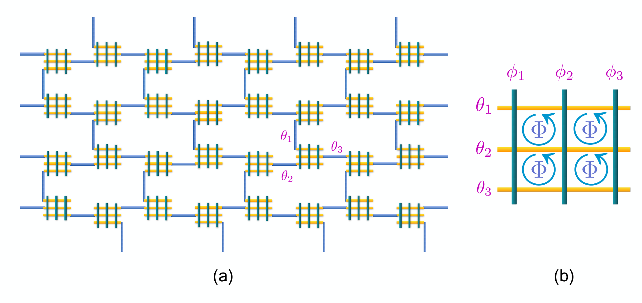
Consider an array of superconducting wires as shown in Fig. 1. An elementary building block depicted in Fig. 1(b) consists of three horizontal “gauge” wires and three vertical “matter” wires coupled via Josephson junctions, forming a “waffle” like geometry. We further introduce an external magnetic flux threading each plaquette of an elementary waffle , where is an integer and is the flux quantum. 11 1 In a more realistic experimental setup, instead of threading flux through the plaquette loops, one can instead replace the single Josephson junction between two crossing wires by ancillary loops forming a highly-asymmetric DC SQUID. The phase shift encoded in the matrix can be controlled by tuning the flux biases in the two arms of the SQUID. We refer readers to Ref. Chamon et al. 2020b for a more detailed discussion on the experimental perspective. The full array forms a two-dimensional honeycomb lattice with a waffle at each lattice site, and an extended gauge wire at each link. Notice that the gauge wires are shared between the sites whereas the matter wires are localized on each lattice site. Denoting the superconducting phases of the gauge wires as and the matter wires as , the Hamiltonian of such an array can be written as
| (1) |
where the Josephson coupling
| (2) |
and the capacitance term
| (3) |
In the above equations, is the Josephson energy of the junctions, the vector denotes the charge of each gauge wire and matter wire , and is a capacitance matrix of the waffle. The charges and phases are conjugate variables satisfying the standard commutation relations and .
II.1 Combinatorial gauge symmetry
The magnetic flux threading each plaquette of the waffle enters the Josephson coupling as a phase shift, which is encoded in the coupling matrix in Eq. (2). To see the phase shift in the Josephson coupling energy between each pair of crossing wires and , one simply needs to count the total flux piercing the rectangle formed by wires . For example, consider the Josephson coupling energy between gauge wire and matter wire . This coupling acquires a phase shift in the presence of a flux : . This corresponds to matrix element in Eq. (2). Similarly, the phase shift between wire and any matter wire , as well as wire and any gauge wire , is zero, since there is no loop formed in this case, which corresponds to . One can readily check that the coupling matrix in Eq. (2) has the following form:
| (4) |
where and . One recognizes that the matrix above is precisely the discrete Fourier transform matrix with entries , which is also a complex Hadamard matrix satisfying . Complex Hadamard matrices of the form (4) are invariant under a pair of left/right monominal transformations, which underlie the combinatorial gauge symmetry. Specifically, has the following automorphism
| (5) |
where and are monomial matrices. Equivalently, and generate permutations and shifts of the superconducting phases on the gauge and matter wires within a waffle, respectively:
| (6a) | ||||
| (6b) | ||||
under which the Josephson coupling terms in the Hamiltonian of a single waffle is invariant. We further restrict the matrix to be diagonal, since the gauge wires on the lattice are shared between sites and cannot be permuted. It turns out that if we take to be of the following form
| (7) |
then is also a monomial matrix
| (8) |
One can further check that is monomial for any permutation along the diagonal of the matrix. Notice that is uniquely determined for a given , following from the automorphism Eq. (5). Permutations of the matter wires are allowed on the lattice because the matter wires are localized on each site, and permutations simply correspond to relabeling the wires. Physically, the transformation corresponds to a phase shift on two out of the three gauge wires within a waffle, such that the product is preserved.

The automorphism of under monomial transformations naturally furnishes a local gauge symmetry on the full lattice. One can construct the following operator generating a local gauge transformation around an elementary hexagonal plaquette on the lattice, as depicted in Fig. 2:
| (9) |
where generates permutations and phase shifts of the matter wires located on site according to Eq. (6b): , and generates phase shifts on the two gauge wires emanating from site : . The automorphism of directly leads to the invariance of Hamiltonian (2) under : , for all . Furthermore, the local gauge transformations on different plaquettes commute with one another: . Thus we have shown that the system in the classical limit where only is present has a local gauge symmetry. Next, we will show that the capacitance term is also invariant under .
The capacitance matrix contains the following entries: the self-capacitances of a single gauge wire, , and of a single matter wire, ; the capacitance of the Josephson junction, ; and the mutual-capacitance between two neighboring wires that are parallel to one another, . The capacitance is the smallest of all, as can be easily inferred from the geometry if the wires are thin and widely separated compared to their width. Neglecting yields a capacitance matrix that is invariant under the permutation of the indices of the matter (as well as gauge) wires. This symmetry carries to the inverse matrix that controls the charging energies. 22 2 We remark that a small value of breaks the permutation symmetry among the three matter wires; nevertheless, if Hamiltonian (1) supports a gapped phase with topological order, it will remain stable in the presence of a small combinatorial symmetry breaking perturbation so long as the gap stays open. In practice, one can also design the geometry of the wires, such that the ’s between different wires are symmetrized. See Ref. Chamon et al. 2020b for details.
Since the charge and superconducting phases are conjugate variables, the phase shift in the monomial transformations is generated by the unitary operators
| (10) |
acting on the gauge and matter wires, respectively. Because these unitary operators trivially commute with the charge operators and , and is invariant under the permutation of the matter wires, we conclude that . Combining with the previous finding that , it follows that . Hence the full lattice Hamiltonian (1) is a gauge theory with local combinatorial gauge symmetry.
II.2 Minima of on a single waffle

Having established the local combinatorial gauge symmetry of Hamiltonian (1), we shall now look at the minima of the classical potential energy on a single waffle. We will show that the superconducting phases of the gauge wires at the potential minima are -valued. Therefore, when the Josephson energy is the dominant scale, Hamiltonian (1) can be effectively described in terms of variables, from which the topological phase emerges.
Minimizing the Josephson energy ties together the and phase variables (see details in Appendix A),
| (11) |
The minimum energy is given by
| (12) |
We plot the potential profile as a function of and while fixing in Fig. 3(a). We find six (three inequivalent) degenerate minima with corresponding to and being 0 or , such that or . In Fig. 3(b), we show all six inequivalent gauge wire phase configurations corresponding to the minima of the potential energy. For each configuration shown in Fig. 3(b), there are another two equivalent ones from permuting the three phases, yielding a total of 18 ground state configurations. Notice that the three degenerate maxima in Fig. 3(a) with also correspond to being 0 or , but now with instead.
Turning on the capacitance term introduces quantum fluctuations in the phases. When the Josephson energies are larger than the charging energies, induces tunneling between nearest-neighboring minima, which corresponds to an instanton in Euclidean spacetime. In Fig. 3(a), we show two examples of such tunneling processes at leading order, where one of the three phases is shifted by while the other two remain unchanged. Semiclassically, the amplitude of such a tunneling process can be estimated from the Euclidean action of the instanton (or equivalently, the WKB approximation). We provide detailed calculations in Appendix B, which lead to a tunneling amplitude , where is an effective capacitance dependent on , and . Notice that this amplitude already takes into account the shifts in , which, when is large, follow the instantaneous minimum of and is hence locked to according to Eq. (11).
The minima depicted in Fig. 3 suggest that the system admits an effective representation in terms of -valued operators at low energy. We place a degree of freedom on each bond of the honeycomb lattice (Fig. 4), and introduce clock operators and satisfying the algebra
| (13a) | |||
| (13b) | |||
In the basis where is diagonal, represents the three possible gauge wire phases at the potential minima. The capacitance-induced tunneling can be represented by a transverse field that shifts the eigenvalue by . In terms of the clock variables, the superconducting wire array can be described effectively at low energy by
| (14) |
where , , and . The generator of local gauge transformation (9) now takes the form and around a hexagonal plaquette, as shown in Fig. 4. It is easy to verify that for any , ; hence . With periodic boundary conditions, and satisfy the following constraints:
| (15) |
where and denote two sublattices of the honeycomb lattice. In Appendix C, we show explicitly that Hamiltonian (14) with the gauge constraint imposed by is equivalent to the quantum double model Kitaev 2003. However, since , the star term in Hamiltonian (14) energetically favors or , while has a higher energy. In other words, we are sitting within a non-zero mixed flux sector of the quantum double model due to the inverted potential. As we will see in the next section, this key distinction from the conventional quantum double model has important consequences on the phase diagram of the system, and in particular, on how the topologically ordered phase emerges. In Appendix F, we also provide a matrix leading to the usual quantum double where the star term favors the zero-flux sector .

III topologically ordered phase from bond dimerization

We shall now discuss the phases that Hamiltonian (14) sustains. For the conventional quantum double model with a in front of the star term, one expects a gapped phase with topological order for . However, the situation is drastically different for an inverted potential with a in front as in Hamiltonian (14). Let us start by counting the ground state degeneracy in the limit (or ), and when the gauge constraint is imposed. Denote the total number of vertices, bonds, and plaquettes on the honeycomb lattice as , , and , respectively. The ground state degeneracy of Hamiltonian (14) on a torus in the large limit is
| (16) |
where we have used the relations , and the -1’s on the exponents account for the constraint (15). This indicates that the ground state is massively degenerate, and that the gauge constraint cannot fully lift this degeneracy. We will show in the next section that upon further turning on a weak uniform transverse field , the system can be mapped to a quantum spin- XY model which is in fact gapless. Therefore, due to the inverted potential, Hamiltonian (14) as it is does not support a gapped topological phase.
Nevertheless, a gapped topological phase emerges with a slight modification of Hamiltonian (14). Instead of a uniform transverse field, we apply a strong transverse field on the vertical bonds forming the hexagonal lattice, and a weak transverse field on all other bonds with while keeping both and much smaller than . (Notice that the WKB calculation yields an exponential suppression in the tunneling amplitudes and . Thus it is experimentally feasible to have and smaller than Chamon et al. 2020b.) This leads to a bond dimerization pattern depicted in Fig. 5(a). Now the Hamiltonian takes the form
| (17) | |||||
We start by considering the limit when . In this limit, the system becomes a set of decoupled dimers formed by the strong bonds, since the weak bonds have no dynamics. In Fig. 5(b), we show the energy levels associated with a single dimer in the limit of infinite . In the absence of , the ground state of the single dimer is four-fold degenerate in corresponding to each or , which is the source of the massive ground state degeneracy in Eq. (16). The excited states correspond to flipping either or both stars to , which is separated from the ground state subspace by a large energy of order . Upon turning on , the four degenerate ground states will split, and the unique ground state, in the star variables, is , whose energy is lowered by . To show that the massive degeneracy on the full lattice is indeed split, we compute the ground state degeneracy in this case:
| (18) |
where the additional factor of corresponds to one constraint per unit cell imposed by , and the total number of unit cells is equal to . We find that the ground state indeed has a nine-fold topological degeneracy on a torus, which coincides with that of the conventional quantum double.
In the above countings, the gauge constraint is imposed by hand. In our model, such a plaquette term can be generated perturbatively upon turning on , yielding an associated energy scale corresponding to the vison gap. Here we point out another key distinction from the usual quantum double with a in the Hamiltonian. In that case, a plaquette term is generated only at sixth order in in degenerate perturbation theory, yielding a very small vison gap when . The reason for such a small vison gap is that creates star excitations with a large energy cost of order , which suppresses the gap. In our model (17) with an inverted potential and dimerized transverse fields, however, one does not have to pay an energy of order to create an excitation. Rather, there are cheaper excitations one can make that only cost an energy of order , which correspond to transitioning between the ground state and first excited state in the presence of as shown in Fig. 5(b). Furthermore, the plaquette term now can be generated at fourth order in , leading to a larger vison gap than in the usual quantum double. 33 3 We remark that because the resulting vison gap is small compared to the scale , it would be difficult in practice to attain low enough temperatures to reach the true ground state, or even a thermal state with a low density of visons. Nonetheless, there may still be signatures of the mutual statistics of the spinons and visons that could be observed in the regime where temperature is larger than the vison gap but still much smaller than the spinon gap, as discussed (for the model) in Ref. Hart et al. 2021.
We compute the plaquette term from Hamiltonian (17) using degenerate perturbation theory. In Fig. 6 we show a fourth-order process in which a pair of excitations is created and annihilated around a plaquette. In the absence of , the ground state written in terms of star variables is a tensor product of on all strong bonds. Applying on a weak bond shifts the two stars connected to the weak bond by or . For example, consider the action of a weak transverse field on a bond connected to of a dimer in its ground state:
| (19) |
where the last two states cost an energy of order and can be projected out in the limit of infinite . The first two states, on the other hand, are low energy excitations with energy only. Define the projector onto the low energy subspace: . One can thus compute the effective Hamiltonian at fourth order in acting within the ground state subspace. For example, the process shown in Fig. 6 gives a contribution to the effective Hamiltonian:
| (20) |
There are in total 24 different fourth-order processes of pair creations and annihilations around a plaquette, and contributions from all other processes can be calculated in a straightforward manner. The important point here is that the perturbative vison gap is fourth order in as opposed to sixth order in , and hence can be made significantly larger than that in the usual quantum double. In Appendix D, we provide numerical results of Hamiltonian (17) on an elementary “spider” like geometry, and compare with the conventional quantum double with . The numerical results indeed suggest that a larger gap can be achieved in our model.
To conclude, Hamiltonian (17) sustains a gapped phase with topological order upon introducing strong and weak transverse fields as depicted in Fig. 5. Our analysis above mainly focuses on the perturbative regime where , but we expect the topological phase to persist for , and . For , the transverse field dominates and the system becomes a trivial paramagnet. In the next section, we will consider the regime where , and .
IV Quantum XY-ordered phase
Now that we have established the existence of a topological phase in our system, let us now consider what happens if becomes greater than while both and are small. In this regime, since the star operator still has a non-zero expectation value in the ground state, it is useful to consider a dual description of Hamiltonian (17) in terms of clock degrees of freedom on the vertices of the honeycomb lattice, which we have been implicitly using in the previous section. In this section, we shall first show a duality mapping from Hamiltonian (17) to a quantum three-state Potts model. In the dual picture, the isotropic point maps to a quantum spin- XY model with XY ordering in the ground state and a gapless spectrum Kennedy et al. 1988; Sandvik and Hamer 1999. For , we consider the limit , when the system maps to decoupled XY chains. A small couples the chains, and we analyze the effect of inter-chain couplings using abelian bosonization. We find that the inter-chain coupling due to a weak is marginal around the decoupled chain fixed point, and hence the system should remain gapless for a non-zero but weak .

IV.1 Duality mapping: quantum three-state Potts model
The duality we demonstrate here is in close analogy with the familiar Kramers-Wannier duality between the two-dimensional transverse field Ising model and the quantum double Wegner 1971. Define clock degrees of freedom and on each vertex of the honeycomb lattice, and the following duality tranformations (shown in Fig. 7):
| (21a) | ||||
| (21b) | ||||
| (21c) | ||||
where denotes the bond connecting adjacent vertices sublattice and sublattice . Notice that a single operator is expressed as a string operator in terms of the gauge degrees of freedom:
| (22) |
where denotes an arbitrary path starting from a link emanating from site and ending at infinity. The string operator involves alternating and , and we choose the convention that a string with endpoint on sublattice ends with , and a string with endpoint on sublattice ends with . With this convention, one can readily check that the dual variables and satisfy the correct commutation relations for clock variables. In terms of the dual variables, Hamiltonian (17) maps to
| (23) | |||||
Hamiltonian (23) describes a clock model with ferromagnetic interactions, which is equivalent to a three-state Potts model.
One can further check that Hamiltonians (17) and (23) indeed have the same Hilbert space dimension, although naively the quantum double seems to have more degrees of freedom. The Hilbert space dimension of the Potts model (23) is . On the other hand, the quantum double subject to the gauge constraint has a Hilbert space dimension of . Again using the relations among , and on a honeycomb lattice, one finds .
IV.2 Reduction to quantum XY model
Based on Hamiltonian (23), the system admits a simpler description in the regime that we are interested in. In this regime, each can only take values or in the ground state, which can be modeled as a two-level system. Define the Pauli spin operator if , and if . A pair of nearest-nerighbor spins is flippable under the ferromagnetic term in Hamiltonian (23) only if they are opposite. This leads to the following low energy effective Hamiltonian:
where we have introduced the short-hand notations and for a bond that is or is not vertical, respectively. In particular, at the isotropic point , the system maps to an isotropic quantum spin-1/2 XY model. The spin-1/2 XY model is known to have long-range order in the ground state in dimensions greater than one, and the spectrum is gapless Kennedy et al. 1988; Sandvik and Hamer 1999. Moreover, in Appendix E we show that the XY phase is stable in the regime starting from weakly coupled chains, using bosonization techniques.
These results underscore the necessity of a strong dimerization with to stabilize the topological phase, as discussed above. We conclude with a schematic of the phase diagram of Hamiltonian (17) in Fig. 8.
V Mean field theory in the bond-operator representation
(a)
(b)
We now present a mean field theory that is capable of capturing the phase transition between the topological phase and the XY-ordered phase. Such a mean field theory is most conveniently formulated in the dual model (23). Since is large in this regime, we can again work with a truncated Hilbert space with two states per site: and . From our previous discussions in Sec. III, deep inside the topological phase, the system essentially forms dimers on the strong bonds, and the vertices within a dimer are strongly entangled. Therefore, we shall formulate our mean field theory using the bond-operator representation Sachdev and Bhatt 1990. The variational wavefunction is then chosen as a tensor product of dimers on the vertical bonds in the bond-operator basis.
The four states in the Hilbert space of a bond can be combined to form singlet and triplet states:
| (25) |
We take the following variational ansatz of the wavefunction
| (26) |
We expect such a variational wavefunction to be a good ansatz for the actual quantum state deep in the topological phase when . The variational energy per unit cell is
| (27) |
Notice in the above expression that only terms on the third line depend on the phases of the variational parameters, while all others only depend on their norms. Thus, we may choose the phases of the variational parameters such that the third line is minimized. Let us define , and , and rewrite the third line as . This term is minimized when , the phases of and are equal, and the phases of and are equal. One can then use the freedom in the global U(1) phase of the wavefunction to set both and to be real, which also fixes and to be purely imaginary. Let us now define real parameters: , , , and , in terms of which the variational energy becomes
| (28) |
where we have used the normalization condition of the wavefunction. When and are both positive, there are always two local minima of the variational energy at
However, when , which lies outside the domain . Therefore, when , the true minimum is achieved at the boundary, where .
This gives us the phase transition in the mean field theory. When , the ground state is , consistent with the scenario in the topological phase that we discussed in Sec. III. When , the ground state has and taking a value less than , which means that becomes non-zero. Moreover, the variational energy minimum only depends on , hence forming a “Mexican hat”-like profile with O(2) symmetry on top of which an XY-ordered phase can emerge from fluctuations beyond mean field.
While the above simplification in the infinite limit allows for an elegant analytical treatment for the phase transition, we further perform numerical minimization of the variational energy by including all nine basis states associated with a bond in the variational wavefunction. We use the total weight of the components in the ground state wavefunction as an indicator of the phase transition, which is equal to . The results are shown in Fig. 9. Again, we find a critical beyond which a non-zero emerges in the ground states, indicating the transition from the topological phase into the XY-ordered phase. Notice that the paramagnetic phase shown in Fig. 8 is absent in the mean field calculations. The paramagnetic phase corresponds to the ferromagnetically ordered phase in the dual model, for which the variational ansatz (26) is no longer a good one. Hence our mean field theory does not capture the transition into the paramagnetic phase.
VI Summary and outlook
In this paper we presented a realization of a quantum double through a Hamiltonian with only physical interations, namely the Josephson couplings and the capacitances of a superconducting wire array. The construction hinges on the combinatorial gauge symmetry of the Hamiltonian: both the Josephson and capacitive terms are invariant under left/right monomial transformations. This invariance allows the construction of strings of operators that generate an exact local gauge symmetry.
We discussed in detail the consequences of having an inverted star potential in the quantum double model, and the dimerizations that lead to a topologically ordered ground state versus those that stabilize a quantum XY-ordered state. We obtained the phase diagram of the model as function of parameters and that microscopically are tied to the capacitances and the Josephson energy scale . We show that another consequence of the inverted star potential is that the vison gap can be larger than that in the uninverted case, as it occurs to lower order in perturbation theory and as a function of a larger dimensionless ratio (, instead of ).
Our work opens fronts to tackle the problem of realizing quantum double models with realistic interactions that span beyond the specific construction for the group in superconducting arrays. As a simple example, once one obtains the Hadamard matrices using the complex numbers (that originate from fluxes in the superconducting realization), one can easily construct spin-1/2 systems with one- and two-body interactions with the necessary combinatorial symmetry to realize the same quantum double. It then remains to be investigated whether the model supports a gapped phase with topological order. That this spin representation is possible follows from replacing these complex numbers by their permutation representations:
| (29) |
The matrix then becomes a matrix, invariant under pairs of left/right monomial transformations as in (5), which are now represented by permutation matrices. This matrix of interactions corresponds to spin interactions between 9 matter spins at the sites of the honeycomb lattice, with 3 gauge spins at each of the links emanating from each site. While this may appear an unlikely model to encounter in nature, we stress that these kinds of couplings are the same as those used to embed the model in the D-Wave DW-2000Q quantum device Zhou et al. 2020. Embedding the model in such devices is not unrealistic, specially if one explores newer architectures with larger qubit connectivities, such as those in the D-Wave Advantage device.
On yet a different level, the successful construction of the quantum double on top of combinatorial gauge symmetry is not an end on itself, but simply points to the promise that other quantum doubles – Abelian and, more interestingly, non-Abelian – could be constructed. The search for realistic models with at most two-body interactions acquires a systematic path: one must first find coupling matrices with elements in a given group that are invariant under multiplication on the left/right by monomial matrices with elements in . If the condition is further satisfied by right matrices that are diagonal, with only two of the elements along the diagonal not equal to 1, loops can be constructed defining a local gauge symmetry. Once this abstract step of constructing such coupling matrices succeeds, one can find a monomial representation of the group elements and consequently translate the abstract model to a spin Hamiltonian with at most two-body interactions. The pursuit of this generic pathway to constructing quantum doubles for different groups is a possibility that this paper raises.
Acknowledgments
We thank Andrew J. Kerman for a discussion on superconducting arrays on the honeycomb lattice that stimulated this work. We thank Garry Goldstein and Andrei Ruckenstein for constructive criticism and useful discussions. In particular, we thank Garry Goldstein for pointing out to us a correction to the calculation in Eq. 20. Z.-C. Y. would like to thank Jyong-Hao Chen for useful exchanges on bosonization. Z.-C. Y. acknowledges funding by the DoE ASCR Accelerated Research in Quantum Computing program (award No. DE-SC0020312), U.S. Department of Energy Award No. DE-SC0019449, DoE ASCR Quantum Testbed Pathfinder program (award No. DE-SC0019040), NSF PFCQC program, AFOSR, ARO MURI, AFOSR MURI, and NSF PFC at JQI. Z.-C. Y. is also supported by MURI ONR N00014-20-1-2325, MURI AFOSR, FA9550-19-1-0399, and Simons Foundation. This work was supported in part by DOE Grant No. DE-FG02-06ER46316 (H. Y. and C. C.) and by NSF Grant DMR-1906325 (C. C.).
Appendix A Minimum of the Josephson potential
We seek the minimum of the Josephson potential
| (30) |
Let us denote and . The potential minima, subject to the constraint , can be found by minimizing the function
| (31) | |||||
where and are Lagrange multipliers. Taking the derivative with respect to yields
| (32) |
Using the fact that is a pure phase, and is real, we obtain
| (33) |
The minimal energy can be written as
| (34) | |||||
Eq. (34) implies that the Josephson energy minima are given by the gauge wire phase configurations such that the potential
| (35) |
is minimized. Notice from Eq. (32) that the matter wire phases are completely tethered to . Using the fact that at the minima, one can solve for for a given set of via
| (36) |
Appendix B Estimate of the tunneling amplitude from Euclidean action of the instanton
We estimate the amplitude for tunneling between adjacent minima as shown in Fig. 3. As we discussed in Sec. II.2, such processes correspond to shifting the superconducting phases of one gauge wire by while keeping the other two unchanged, thus it gives an estimate for the transverse field strength in the effective Hamiltonian (14).
The Euclidean action for a single waffle is written as:
| (37) | |||||
where the potential energy
| (38) |
and the kinetic energy
| (39) | |||||
As we mentioned in the main text, a small value of breaks the permutation symmetry among the three matter wires; nevertheless, if Hamiltonian (1) supports a gapped phase with topological order, it will remain stable in the presence of a small combinatorial symmetry breaking perturbation so long as the gap stays open.
Due to the combinatorial symmetry, it suffices to consider one particular tunneling process, e.g. the horizontal arrow depicted in Fig. 3(a) where changes from to 0, and , . Throught the tunneling process, all three ’s will change. However, their trajectories are completely fixed by that of the varying , following from Eq. (11). Thus, one may write
| (40) |
where we have suppressed the gauge wire subscript in . The Lagrangian can be simplified as
| (41) | |||||
where we have defined an effective capacitance , and is given by Eq. (34), which is the profile plotted in Fig. 3(a). A particle initially at one minimum of has energy . From energy conservation (in Euclidean space), one obtains:
| (42) |
Hence, the Euclidean action corresponding to this classical trajectory is given by
| (43) |
and the tunneling amplitude is .
In principle, the effective potential is not a constant along the trajectory, due to the -dependence in . Nevertheless, a straightforward calculation of Eq. (11) yields the following simple relations between and :
| (44a) | ||||
| (44b) | ||||
| (44c) | ||||
We find that both and are in fact constant. Therefore as an approximation, we may take to be a constant along the trajectory. Evaluating the action numerically yields the tunneling amplitude .

Appendix C Equivalence between Hamiltonian (14) and quantum double model
We show that Hamiltonian (14) with the gauge constraint is equivalent to Kitaev’s quantum double model in the non-zero flux sector. Since our gauge transformation ’s are defined on the plaquettes, the corresponding quantum double model is most conveniently formulated on the dual triangular lattice, as depicted in Fig. 10.
Let us define an orthonormal basis on each link of the triangular lattice: . The construction of starts from the following group-element-indexed linear operators acting on the above Hilbert space Kitaev 2003
| (45) |
where . And similarly, one can define and , which, for abelian groups, are simply and . In terms of the clock operators, and have the explicit form
| (46a) | ||||
| (46b) | ||||
One can further check that the above operators and satisfy the commutation relation
| (47) |
from which all other commutation relations involving and follow. We further choose an orientation rule on the triangular lattice as depicted in Fig. 10, such that the arrows go clockwise (counterclockwise) around every upward (downward) pointing triangle. For each vertex and the bonds emanating from , we take if the arrow is pointing towards , and otherwise. For each plaquette and the bonds surrounding , we take if is to the left of the bond following the arrow, and otherwise. Using the above rules, one can construct the generators of as follows
| (48a) | ||||
| (48b) | ||||
where the labels are shown in Fig. 10. In terms of the above generators, one can write down the star term, which has the form of a projector Kitaev 2003:
| (49) |
and the plaquette term
| (50) |
Notice that in the usual quantum double model, the plaquette term enforces a zero flux: . Here instead favors sectors with flux or , which corresponds to the inverted potential in Hamiltonian (14). Finally, we can write down the Hamiltonian for the quantum double model :
| (51) |
Going back from the dual triangular lattice to the honeycomb lattice, this is precisely Hamiltonian (14) in the absence of a transverse field and with the gauge constraint imposed.

Appendix D Numerical results of Hamiltonian (17) on a “spider” like geometry
We show exact diagonalization results of Hamiltonian (17) on an elementary “spider” like geometry depicted in Fig. 11. Since one can tile the entire two dimensional honeycomb lattice using the spider as an elementary building block, the spider can be thought of as a minimal lattice on which one can test our model numerically.
As shown in Fig. 11, we fix the 8 external leg configurations , and diagonalize the spectrum of the 8 internal clock degrees of freedom under Hamiltonian (17). We can interpret this particular setup as a single plaquette embedded in the lattice environment, whose configurations are fixed one at a time. There are in total possible external leg configurations that one can fix to. From energetic considerations in the regime as we discussed in Sec. III, the ground state forms dimers on the strong bonds. Therefore, we expect that the ground state energy of the spider is minimized when
| (52) |
Notice that for the entire system on a torus, the above equation is an identity that imposes a constraint on the spectrum; here it arises from energetics instead. Applying Eq. (52) on a spider, we obtain
| (53) |
Out of the external leg configurations, Eq. (53) yields configurations such that the ground state energy is minimized. We have tested that fixing the external legs to be any of the configurations satisfying Eq. (53) yields the same ground state and first excited state energies, which is a direct consequence of the gauge symmetry.
In Fig. 12, we plot the energy gap between the ground state and the first excited state as a function of , for fixed and , and external leg configuration satisfying Eq. (53). This can be viewed as the vison gap obtained numerically from a spider building block. In our model where , we find that the fitted gap scales as for small , which is consistent with our perturbative calculations in Sec. III. As a comparison, we also plot in Fig. 12 the energy gap for Hamiltonian (17) with , which corresponds to the conventional quantum double model with zero flux. In this case, we find a much smaller vison gap than in Fig. 12(a) with an inverted potential. The plaquette term for is generated at sixth order in perturbation theory, which leads to a small vison gap.
Appendix E Weakly coupled chain limit: bosonization
Another interesting regime that can be understood is when . In the limit when , the system becomes a set of decoupled chains extending along the horizontal direction, as can be seen from Fig. 5(a). Since each chain is described by an XY model, which is equivalent to free fermions in one dimension, the system is apparently gapless in this limit. A weak introduces inter-chain couplings along the vertical direction. We shall now study the effect of this inter-chain coupling using abelian bosonization.
Consider a two-leg ladder shown in Fig. 13, which is described by the following Hamiltonian:
| (54) |
where describes the decoupled chain for . In terms of bosonic fields, the bosonized decoupled chain Hamiltonian can be written as:
| (55) |
where is the dual variable of (not to be confused with the superconducting phases). We have ignored the Luttinger parameter , as well as a prefactor of . To derive the bosonized form of the inter-chain coupling , we need the bosonized form of the spin operators. First, recall the Jordan-Wigner transformation:
| (56a) | ||||
| (56b) | ||||
In the continuum limit, the fermion operator expanded near can be written as:
| (57) |
where describes right and left movers. Finally, we need the following bosonization dictionary Fradkin 2013; Gogolin et al. 2004:
| (58a) | ||||
| (58b) | ||||
| (58c) | ||||
where we have suppressed the chain index for now. Using the above expressions, we can now derive Giamarchi 2003; Vekua et al. 2003:
| (59) | |||||
and similarly for . The inter-chain coupling:
| (60) |
can now be readily bosonized. Introducing the following new variables corresponding to the symmetric and antisymmetric sectors:
| (61) |
the full Hamiltonian can be written as:
| (62) |
where
| (63a) | ||||
| (63b) | ||||
| (63c) | ||||
In the above expressions, we only keep the slowly varying, non-staggered contributions. We find that a term is generated in the antisymmetric sector by the inter-chain couplings. This term has a scaling dimension of , which is relevant. Thus, the antisymmetric sector becomes gapped. To determine the fate of the sector, we may replace by its expectation value:
| (64) |
Then the term has a scaling dimension of , which is marginal. Therefore, we find that the system should remain gapless for a non-zero but weak .
Appendix F A quantum double with an uninverted star term

We give an explicit construction of the usual quantum double with a star term favoring . Consider the Josephson energy (2) with the following matrix:
| (65) |
The corresponding superconducting wire array now contains 6 matter wires and 3 gauge wires per lattice site (“waffle”). The above matrix satisfies , and has the following automorphism
| (66) |
where and are monomial matrices. Hence, the Josephson energy is invariant under transformations (6) on and . We again restrict to be diagonal matrices that do not change the product of the three gauge wire phases at each vertex. For example, if we take a matrix
| (67) |
and a matrix
| (68) |
it is easy to check that the automorphism (5) holds. In Fig. 14(a), we plot the potential energy profile Eq. (12) for the matrix (65), which shows the minima of the Josephson energy. We find that the minima now correspond to gauge wire phases with a zero net flux . In Fig. 14(b), we show all inequivalent gauge wire phase configurations at the potential minima. Therefore, the effective description of the star term now has the usual form: with .
References
- Tsui et al. (1982) D. C. Tsui, H. L. Stormer, and A. C. Gossard, Phys. Rev. Lett. 48, 1559 (1982).
- Laughlin (1983) R. B. Laughlin, Phys. Rev. Lett. 50, 1395 (1983).
- Saminadayar et al. (1997) L. Saminadayar, D. C. Glattli, Y. Jin, and B. Etienne, Phys. Rev. Lett. 79, 2526 (1997).
- de Picciotto et al. (1997) R. de Picciotto, M. Reznikov, M. Heiblum, V. Umansky, G. Bunin, and D. Mahalu, Nature 389, 162 (1997).
- Nakamura et al. (2020) J. Nakamura, S. Liang, G. C. Gardner, and M. J. Manfra, Nature Physics 16, 931 (2020).
- Bartolomei et al. (2020) H. Bartolomei, M. Kumar, R. Bisognin, A. Marguerite, J.-M. Berroir, E. Bocquillon, B. Plaçais, A. Cavanna, Q. Dong, U. Gennser, Y. Jin, and G. Fève, Science 368, 173 (2020).
- Wen (1990) X. G. Wen, International Journal of Modern Physics B 04, 239 (1990).
- Kitaev (2003) A. Y. Kitaev, Annals of Physics 303, 2 (2003).
- Chamon et al. (2020a) C. Chamon, D. Green, and Z.-C. Yang, Phys. Rev. Lett. 125, 067203 (2020a).
- Zhou et al. (2020) S. Zhou, D. Green, E. D. Dahl, and C. Chamon, Experimental realization of spin liquids in a programmable quantum device (2020), arXiv:2009.07853 [cond-mat.str-el] .
- Chamon et al. (2020b) C. Chamon, D. Green, and A. J. Kerman, A superconducting circuit realization of combinatorial gauge symmetry (2020b), arXiv:2006.10060 [quant-ph] .
- Ioffe and Feigel’man (2002) L. B. Ioffe and M. V. Feigel’man, Phys. Rev. B 66, 224503 (2002).
- Douçot et al. (2003) B. Douçot, M. V. Feigel’man, and L. B. Ioffe, Phys. Rev. Lett. 90, 107003 (2003).
- Douçot et al. (2004) B. Douçot, L. B. Ioffe, and J. Vidal, Phys. Rev. B 69, 214501 (2004).
- Hart et al. (2021) O. Hart, Y. Wan, and C. Castelnovo, Nature communications 12, 1 (2021).
- Kennedy et al. (1988) T. Kennedy, E. H. Lieb, and B. S. Shastry, Phys. Rev. Lett. 61, 2582 (1988).
- Sandvik and Hamer (1999) A. W. Sandvik and C. J. Hamer, Phys. Rev. B 60, 6588 (1999).
- Wegner (1971) F. J. Wegner, Journal of Mathematical Physics 12, 2259 (1971).
- Sachdev and Bhatt (1990) S. Sachdev and R. N. Bhatt, Phys. Rev. B 41, 9323 (1990).
- Fradkin (2013) E. Fradkin, Field theories of condensed matter physics (Cambridge University Press, 2013).
- Gogolin et al. (2004) A. O. Gogolin, A. A. Nersesyan, and A. M. Tsvelik, Bosonization and strongly correlated systems (Cambridge university press, 2004).
- Giamarchi (2003) T. Giamarchi, Quantum physics in one dimension, Vol. 121 (Clarendon press, 2003).
- Vekua et al. (2003) T. Vekua, G. I. Japaridze, and H.-J. Mikeska, Phys. Rev. B 67, 064419 (2003).