Probing non-affine expansion with light scattering

We first consider one path of light inside a heterogeneous material composed of a medium of refractive index $n_{g}$ and vacuum that is schematically represented in Fig. 2.a. A path may be decomposed into a succession of $N$ linear segments separated by points ${\bf r}_{\nu}$, with $\nu$ an integer index $0\leq\nu\leq N-1$. Let $\nu$ denote the segment joining ${\bf r}_{\nu}$ to ${\bf r}_{\nu^{+}1}$, with $l_{\nu}=\mathinner{\!\left\lVert{\bf r}_{\nu+1}-{\bf r}_{\nu}\right\rVert}$ the length of this segment, and ${\bf e}_{\nu}=({\bf r}_{\nu+1}-{\bf r}_{\nu})/l_{\nu}$ the unit vector along it, as illustrated in Fig. 2.b. We assign to each segment a variable $\eta_{\nu}$ which is $0$ if the segment is in vacuum, and $1$ otherwise, so that the segment lies in a medium of effective refractive index $n_{\nu}=1+(n_{g}-1)\eta_{\nu}$. The optical phase shift between the start and the end of such a path is therefore

with $k=2\pi/\lambda$, and where $\lambda$ denotes the wavelength in vacuum. When the material is deformed, the pathways of light are changed, and the variation of the optical phase shift reads:

where $\delta k$, $\delta l_{\nu}$ and $\delta n_{\nu}$ are the variations of $k$, $l_{\nu}$ and $n_{\nu}$, and we suppose that perturbations are small: $\delta k\ll k$, $\delta l_{\nu}\ll l_{\nu}$, $\delta n_{\nu}\ll n_{\nu}$. We study the phase variations resulting from a direct change of the wavelength and from the deformation of the material occurred with a change in temperature, and then:

In the above equation (3b), we have neglected dispersion effects which would include an additional term $\eta_{\nu}\bigl(\partial n_{g}/\partial\lambda\bigr)\delta\lambda$. Indeed, the contribution of wavelength dispersion to $\delta(kn_{\nu}l_{\nu})$ can be written as $kl_{\nu}\eta_{\nu}(\partial n_{g}/\partial\lambda)\delta\lambda$, which can be compared to $\delta k~n_{\nu}~l_{\nu}=-k~(\delta\lambda/\lambda)~n_{\nu}~l_{\nu}$. For such materials as glasses that are studied experimentally in this work we have $|\frac{\partial n_{g}}{\partial\lambda}|\ll 1/\lambda$. It follows that $kl_{\nu}\eta_{\nu}(\partial n_{g}/\partial\lambda)\delta\lambda\ll\delta k~n_{\nu}~l_{\nu}$. In conclusion, the phase variations due to dispersion effects can be considered as negligible with respect to the phase variations due to a change in $\delta k$.

Since the phase variation $\delta\phi_{N}$ depends on $\delta l_{\nu}$ through Eq. (3c), we now describe the deformation of a material subjected to a thermal expansion. The segment $\nu$ located initially between the points ${\bf r}_{\nu}$ and ${\bf r}_{\nu^{+}1}$ now joins the points ${\bf r}_{\nu}+{\bf u}({\bf r}_{\nu})$ and ${\bf r}_{\nu+1}+{\bf u}({\bf r}_{\nu+1})$ after deformation, where ${\bf u}({\bf r})$ is the displacement field. For small deformations such that $\mathinner{\!\left\lVert{\bf u}({\bf r}_{\nu+1})-{\bf u}({\bf r}_{\nu})\right\rVert}\ll l_{\nu}$ the length variation is then:

We can decompose the differential displacement ${\bf u}({\bf r}_{\nu+1})-{\bf u}({\bf r}_{\nu})$ as the sum of an affine dilatation and a deviation from an isotropic deformation:

where $\alpha$ is the coefficient of linear expansion. Using Eq. (5), the equation (4) becomes:

The decomposition of Eq. (5) is not unique, and we must add an additional constraint to enforce uniqueness. For that purpose, we impose that the non-affine displacement is a part of the displacement which is not correlated with the relative locations of the points ${\bf r}_{\nu}$, and hence is uncorrelated with ${\bf e}_{\nu}$, such that:

where $\sum_{\nu=0}^{N-1}$ (or $\sum_{\nu}$ for the sake of conciseness) represents the summation over all the segments of the considered light path. This constraint may also be written as:

which means that $\alpha\,\delta T$ accounts for the relative increase of the total length of all paths inside the material.

The deviations from affine isotropic deformations are expected to vary linearly with the affine contribution Alexander 1998, and hence with $\delta T$, allowing us to reasonably write:

where we introduce the vector $\bm{\beta}_{\nu}$ which does not depend on $\delta T$, and which verifies $\sum_{\nu}\bm{\beta}_{\nu}\cdot{\bf e}_{\nu}=0$. The phase variation given in Eq. (2) may then be written as:

with

We now calculate the average value of $\big\langle\exp(j\delta\phi_{N})\big\rangle_{N}$, assuming $\big\langle\cdot\big\rangle_{N}$ to be the average of the quantity $\cdot$ over all light paths involving $N$ segments. Since we consider a heterogeneous material which scatters strongly the light, we have $N\gg 1$, and by the central limit theorem, $\delta\phi_{N}$ can be considered as a Gaussian random variable D. J. PineandD. A. WeitzandG. MaretandP. E. WolfandE. Herbolzheomer and P. M. Chaikin 1990; Weitz and Pine 1993, so that Dainty 1989; Goodman 2015:

From Eq. (10), the mean phase shift and its variance may be written as a combination of $\delta T$ and $\delta\lambda/\lambda$, i.e.,

and

where $A$, $B$, $C$ are coefficients whose calculi are given in the Appendix. In the above expressions, and throughout the remainder of this article, we have introduced the following notation $\overline{a}$ for a ”length-average” of any quantity $a_{\nu}$ which depends on segment index $\nu$: $\overline{a}=\big\langle a_{\nu}l_{\nu}\big\rangle/\langle l_{\nu}\rangle$. Similarly, we define a quadratic average as ${\overline{\hbox{$\overline{a}$}}}=\big\langle a_{\nu}l_{\nu}^{2}\big\rangle/\langle l_{\nu}\rangle^{2}$. Since $\big\langle l_{\nu}^{2}\big\rangle\neq\big\langle l_{\nu}\big\rangle^{2}$, beware that $\overline{l}=\langle l_{\nu}l_{\nu}\rangle/\langle l_{\nu}\rangle\neq\langle l_{\nu}\rangle$, and that for any constant $c$: ${\overline{\hbox{$\overline{c}$}}}=\langle c~l_{\nu}^{2}\rangle/\langle l_{\nu}\rangle^{2}=c\langle l_{\nu}^{2}\rangle/\langle l_{\nu}\rangle^{2}\neq c$.

We now suppose that the system is illuminated by a light beam, and we collect the scattered light in a given experimental geometry. We introduce $P(s)$ as the normalized distribution of path lengths and, therefore, the electric field autocorrelation function reads D. J. PineandD. A. WeitzandG. MaretandP. E. WolfandE. Herbolzheomer and P. M. Chaikin 1990; Weitz and Pine 1993:

where $\delta\phi_{s}$ is the phase variation for a light path of length $s$. Identifying $s$ with $N\langle l_{\nu}\rangle$ in the above expression, and using Eqs. (12)-(14), we obtain:

with

The quantity $g_{E}(p)$ is the Laplace transform of $P(s)$. For a plane-parallel slab of thickness $L$ in backscattering geometry, $P(s)$ may be calculated as Vellekoop, Lodahl, and Lagendijk 2005:

with:

where $l^{*}$ is the transport mean free path of the light inside the material, $z_{0}$ is the depth at which the diffusing source is located, and $z_{e}$ is the so-called extrapolation length Vellekoop, Lodahl, and Lagendijk 2005. Finally, $\alpha_{a}$ is a coefficient related to the light absorption inside the material. The intensity correlation function (that we access experimentally in the remainder of the article) is finally related to the electric field autocorrelation function $g_{E}$ using the Siegert relation Goodman 2015:

The experimental setup that we propose to use for sensing non-affine deformations in granular materials represents an arrangement of diffusing wave spectroscopy (DWS) in backscattering configuration and is schematically sketched in Fig. 3. The experiment being based on the fine measure of decorrelation of speckle interference intensity patterns, it was necessary to ensure the best thermal stability of the experiment. In order to reduce the relative displacement between the elements of the setup due to external thermal fluctuations, all the experiment (including laser, camera, regulated thermal cell) is placed into a temperature controlled environment that allows the whole setup to be kept at $22\pm 0.2^{\circ}C$. The scattering material is placed into a thermo-regulated cell. The regulation of the cell is made with a PID controller (Stanford Research PTC10) which ensures a thermal stability of $\pm 3~mK$. In order to minimize thermal drift, the setup (including internal and external thermal regulated cells) was left to equilibrate for at least 24 hours.

The illumination source is a short-wave infrared (SWIR) fibred distributed feedback (DFB) laser (PowerSource 1905 LMI from Avanex, USA) combined with a laser diode controller (LDC-3744, ILX LightWave, USA). This device makes it possible to modulate the incident wavelength from $\lambda=1.5557~\mu$m to $1.55705~\mu$m without mode hopping by finely tuning the temperature of the semiconductor laser chip. The spectral width of the laser diode is $<5$ MHz, giving a coherence length $>60$ m, which is very large compared to the total path length inside the material. This means that the contrast of the speckle pattern does not depend on the spectral width of the laser. The laser beam was used to shine the sample with a circular $6~mm$-diameter laser spot. Upon scattering of light in the diffusing material, the light backscattered out of the sample forms a far-field speckle pattern, whose intensity fluctuations were recorded with an InGaAs SWIR camera (OWL 320, Raptor Photonics, Northern Ireland) that provides $320~$px $~256~$px resolution, with a pixel size of $30~\mu$m $~30~\mu$m. The average size of a speckle spot was measured to be approximately of $\simeq 3$ pixels per speckle.

The sample used in this experiment was a glass frit (grade P2) designed for filtration, and purchased from Bibby Scientific. The thickness of the frit is $L=4.4$ mm, and the volume fraction of glass $\phi_{g}=0.648$ is measured by weighting of the frit. The P2 grade of the frit corresponds to a ”maximum pore size” lying in the range $d_{p}=40-100~\mu$m. Microscopic inspection of the frit shows that it is composed of glass particles with a typical polydispersity of $\sim 3$. The frit is made of Borosilicate Pyrex Glass with the following physical characteristics sch 2014a; sch 2014b: the refractive index at $1.50~\mu$m is $n_{g}=1.456$, with a dispersion coefficient of $(\partial n_{g}/\partial\lambda)=-1.2~10^{-5}$ nm^-1, and the coefficient of the linear thermal expansion is given as $\alpha=3.25~10^{-6}$ K^-1. Few references in the literature were found to assess the value of the thermo-optic coefficient of Pyrex glass, especially in the SWIR range. From references Ramachandran 1947; Peters 1926, the value of the $(\partial n_{g}/\partial T)$ can be expected to lie between $+5~10^{-6}$ and $+10^{-5}$ K^-1 for temperatures in the $20-100^{\circ}C$ range, and for a visible wavelength. According to experiments reported on other types of glassHarris et al. 1977, the value of the thermo-optic coefficient tends to slightly decrease with an increase of the wavelength, but seems to remain of the same order of magnitude. A measure of the thermo-optic coefficient of a borosilicate glass with physical characteristics close to Pyrex has been reported at 1550 nm in Koike and Sugimoto 2006, with a value close to $+9.10^{-6}$ K^-1. In the remainder of this article, we may thus retain an admissible range of $[+5~10^{-6};+10^{-5}]$ K^-1 for the thermo-optic coefficient of Pyrex glass at 1550 nm. It can be noted here that the above numerical values allow us to validate the assumption made in the theoretical model to neglect dispersion effects. Indeed, with $(\delta\lambda)_{max}\sim 100$ pm and $(\delta T)_{max}\sim 15^{\circ}$ K in the experiment reported below, one has $(\delta T)_{max}.\bigl|\frac{\partial n_{g}}{\partial T}\big|\sim 70~(\delta\lambda)_{max}.\bigl|\frac{\partial n_{g}}{\partial\lambda}\big|$.

We obtain the normalized intensity correlation function between two images acquired at $(\lambda_{1},T_{1})$ and at $(\lambda_{2},T_{2})$ from the product of the recorded speckle intensity averaged on all pixels of the camera. However, we observed a drift of the speckle pattern with time even at rest because of the thermal expansion of the temperature regulation cell and due to the long duration of experiments. In order to correct this drift we proceed as follows: let $I_{1}(p)$ and $I_{2}(p)$ denote the raw intensities recorded at pixel $p$ in the image $1$ and $2$, respectively. We construct $I_{2,s}(p,\delta{\bf r})$ as the intensity of the pixel $p$ when the image $2$ is shifted by a quantity of $\delta{\bf r}$ using a cubic-spline interpolation of intensity. Then, we define $g_{I}$ as:

The maximization with respect to $\delta{\bf r}$ is obtained using a Powell maximization scheme Press et al. 2007. The shift $\delta{\bf r}$ corresponding to the maximal correlation is typically smaller than $2$ pixel size (i.e., $60~\mu$m) both in horizontal and vertical directions. However, the coherence area on the camera sensor being $\sim 100~\mu$m, neglecting this shift of the speckle pattern would diminish the correlation and would significantly bias the measurements.

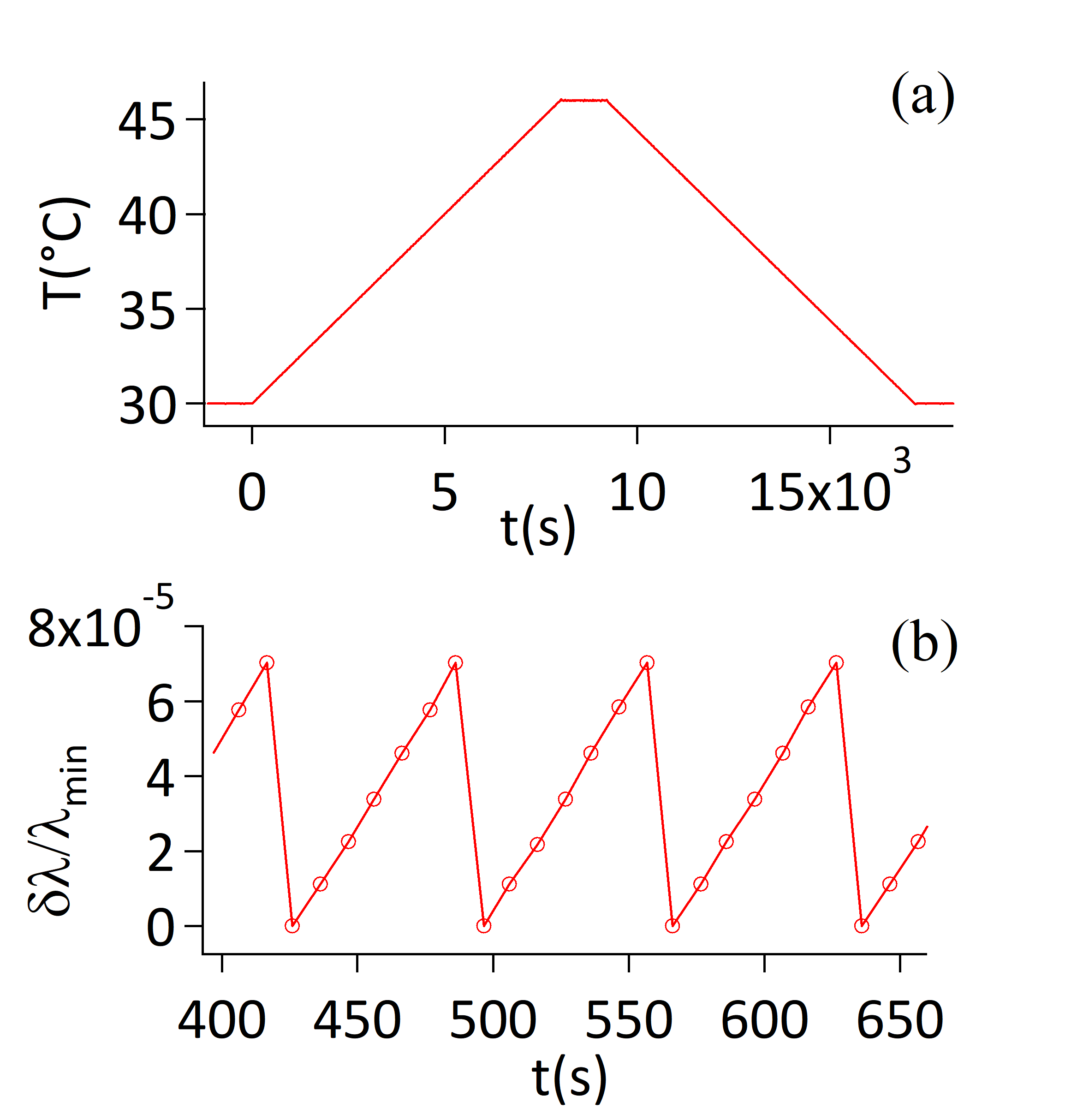
The plots of Fig. 4 summarize a typical experiment. Initially, we keep the sample at the fixed temperature of $30^{\circ}C$ for a few minutes. Then we first increase the temperature with the constant rate of $2~10^{-3}~$K.s^-1 up to $46^{\circ}C$, hold it at $46^{\circ}C$ for several minutes, and finally we decrease the temperature back to $30^{\circ}C$ with the same rate. During this cycle, the laser wavelength is gradually increased from its minimal value $\lambda_{min}$ with steps of $18~$pm every $10~$s, and after $6$ successive steps the wavelength is set back to $\lambda_{min}$. The wavelength scanning cycle is thus approximately 280 times faster than the temperature cycle. Image recording on the camera is performed with a $10~$s period, therefore, during one full temperature cycle, we acquire approximately $1500$ images at different temperatures and wavelengths.

We confirm the reversibility of the sample deformation directly from the intensity correlation function obtained after one full experimental cycle comprising sequential dilatation and contraction of the sample. For this purpose, we correlate an image acquired before the increase of temperature with successive images recorded at the same wavelength. Figure 5 shows the evolution of the intensity correlation function $g_{I}$ as a function of the temperature difference. We obtain $g_{I}(\delta T=0,\delta\lambda=0)\simeq 0.97$ after the temperature cycle indicating a good overall reversibility of the correlation function. We also examine the stability of the recorded signal by performing the experiment in which we keep constant both temperature and wavelength during a few hours. We observe a typical decrease of the correlation of about $0.01$ per hour. We attribute this small decorrelation of the signal to non-ideal thermal control of the environment. From Fig. 5, one can also see that the correlation may be slightly larger for the cooling stage of the sample than for the heating step. This is probably due to a small temporal delay between the measured temperature and the actual temperature inside the sample. Thus, the above tests clearly prove the reversibility of the material deformation under investigation, and that the experiment will address elastic deformations. Therefore, any effect related to an irreversible deformation or a displacement of the sample may be safely neglected as soon as correlation is smaller than $\sim 0.98$ during the temperature increase. We also checked a great reproducibility of the experiment by observing consistent measurements over several consecutive temperature/wavelength cycles.

We now consider in more details the correlation functions $g_{I}(\delta T,\delta\lambda/\lambda)$. These functions may be calculated for every couple of images, but it is very time-consuming and, therefore, we propose several ways to optimise the analysis. First, there are many couples of images corresponding to the same value of $(\delta T,\delta\lambda/\lambda)$. We verified that for such couples the values of $g_{I}$ are the same, and in the following we consider only one couple to obtain $g_{I}(\delta T,\delta\lambda/\lambda)$. Second, one can also see from Eqs. (16)-(20) that there is a symmetry, such that $g_{I}(\delta T,\delta\lambda/\lambda)=g_{I}(-\delta T,-\delta\lambda/\lambda)$. It allows us to consider only correlation function with $\delta\lambda/\lambda>0$. In addition, we computed all correlation functions during the increase of temperature. In practice, if $T_{min}$ and $T_{max}$ are the minimum and maximum temperatures, and $\lambda_{min}$ and $\lambda_{max}$ are the minimum and maximum wavelengths respectively, then $g_{I}(\delta T,\delta\lambda/\lambda)$ is obtained by correlating images of the sample heating at $(T_{min},\lambda_{min})$ and at $(T_{min}+\delta T,\lambda_{min}+\delta\lambda)$ for $\delta T>0$. On the other hand, images recorded at $(T_{min},\lambda_{min}+\delta\lambda)$ and at $(T_{min}-\delta T,\lambda_{min})$ are used to compute the correlation function for $\delta T<0$.

The correlation functions obtained for different values of $\delta\lambda/\lambda$ are shown in Fig. 6. At $\delta\lambda/\lambda=0$, the correlation function logically has a maximum at $\delta T=0$ and it monotonically decreases with temperature variation. It reveals a change in the path lengths induced by thermal expansion of the sample and by variation of the refractive index with the temperature. For a given value of $\delta\lambda/\lambda$, the correlation function is maximal for a non-vanishing value of $\delta T$ and it monotonically decreases with temperature around this maximum. It indicates that some part of the path length changes induced by the same reasons are cancelled in this case by wavelength variations. However, the correlation at maximum is lower than one, and decreases with $\delta\lambda/\lambda$.

We now want to describe the correlation function $g_{I}$ in accordance with the model developed in Section II. The correlation function depends on variables $\delta T$ and $\delta\lambda/\lambda$, and on numerous parameters. The parameters $A$ and $B$, respectively introduced in Eq. (11) and (14), are related to the variation of the optical path lengths with temperature. On the other hand, the parameter $C$ introduced in Eq. (14), as well as $l^{*}$, $z_{0}$, $z_{e}$ and $\alpha_{a}$ characterize the propagation of light inside the material. Some of these parameters can be evaluated directly. In the following, we consider a point zone located at the distance of $z_{0}=l^{*}$ inside the material. The value of $z_{e}/l^{*}$ depends on refractive index of the material. Taking an average refractive index $n_{frit}\simeq 1+\phi_{g}~(n_{g}-1)\simeq 1.31$, we have Vera, M U, Durian 1996 $z_{e}=1.8~l^{*}$. The value of $\alpha_{a}$ is related to the light absorption in the material, and is of very minor importance in practice in our case. Indeed, the effect of the absorption consist in multiplying $P(s)$ by $\exp^{-s/l_{a}}$ with $l_{a}=3/\alpha_{a}^{2}l^{*}$. However, the finite thickness $L$ of the frit effectively cuts the paths longer than $\sim L^{2}/l^{*}$ in $P(s)$. In practice, the better adjustment of the correlation function for $g_{I}\simeq 1$ is obtained for values of the optical length penetration such that $l_{a}\gg L^{2}/l^{*}$, with no sensitivity of the adjustment to the value of $l_{a}$. The parameter $B$ was fixed to its expected value, evaluated from Eq. (44) of Appendix VII.4, i.e., $B\simeq 12$. However, in any case, since $B\,A^{2}\ll C$, it may be seen from Eq. (14) that this parameter does not influence the decay of the correlation function.

The remaining parameters are then $A$, $C$, and $l^{*}$. In the case of our model, a fit of the whole dataset from Fig. 6 using a chi-square minimization algorithm is difficult. We tried to use a Levenberg-Marquardt algorithm, but this led to convergence problems. More precisely, the algorithm fails to converge, or it converges to parameter values that are very close to initial ones. This can be related either to the strong non-linearity of the $g_{I}$ function (for $\delta\lambda=0$ and small $\delta T$, $g_{I}\sim\exp[\sqrt{\delta T}]$, or to the two-dimensional variables for the fitting problem. Because of all these reasons, we adjusted the parameters manually. This can be easily done since different variables play distinct roles. Indeed, the couple $(\delta T,\delta\lambda/\lambda)$ which maximizes the correlation function depends mainly on the parameter $A$, whereas the value of the maximum is governed by $C$. Finally, the decay of the correlation function depends on $l^{*}$. The curves in dashed line in Fig. 6 show the modeled correlation functions with the parameters $A_{exp}=7.3\pm 0.1~10^{-6}$ K^-1, $l^{*}=230\pm 20$ $\mu$m, and $C_{exp}=5\pm 1.0~10^{-8}$ K^-2, where the error bars are subjective.

Let us consider a light ray entering into the sample at a point ${\bf r}_{in}$, exiting at ${\bf r}_{out}$, detected at point ${\bf r}_{d}$ as sketched in Figure 7. We denote by $\phi$ the total optical phase accumulated along the path between the source and the detector. For the sake of simplicity, we suppose normal incidence, and we put the origin at ${\bf r}_{in}$. In addition to the phase shift inside the material, some phase shift occurs due to the displacement of the input, output, and detector points. This additional ”external” phase shift is denoted by $\delta\phi_{ext}$, and reads $\delta\phi_{ext}={\bf k}_{in}\cdot\delta{\bf r}_{in}+{\bf k}_{out}\cdot(\delta{\bf r}_{d}-\delta{\bf r}_{out})$. Under isotropic dilatation, we must have $\delta{\bf r}_{out}=\alpha~\delta T~({\bf r}_{out}-{\bf r}_{0})$ as well as $\delta{\bf r}_{in}=\alpha~\delta T~({\bf r}_{in}-{\bf r}_{0})$, where ${\bf r}_{0}$ is some fixed point in the system. Under normal incidence, we have ${\bf k}_{in}\cdot({\bf r}_{out}-{\bf r}_{in})=0$, and it follows that, after simplification:

The first term of Eq. (29) is related to the possible displacement of the detector, and the second term corresponds to a global translation of the speckle pattern. Those two terms can be cancelled out with an appropriate choice of $\delta{\bf r}_{d}$ as it is done experimentally (see Section III.2). The last term depends on the output point. For a direction of detection near the normal of the sample surface, we have ${\bf k}_{out}=k~(\theta_{x},\theta_{y},-1)$ with $\theta_{x},\theta_{y}\ll 1$, and $\delta\phi_{ext}\simeq-k\alpha\delta T~(\theta_{x}x_{out}+\theta_{y}y_{out})$. The decorrelation due to this phase shift may be written as :

We have introduced the normalized distribution $P(s,x_{out},y_{out})$ of paths with length $s$ exiting at point $(x_{out},y_{out})$. The method for evaluating the integral of Eq. (30) is very similar to Ref. Zhu, Pine, and Weitz 1991. The distribution $P(s,x_{out},y_{out})$ is obtained from the analytical solutions of the diffusion equation. For a diffusing localized source located at $(x=0,y=0,z=l^{*})$, we have Zhu, Pine, and Weitz 1991:

It follows that:

with $p_{ext}=-\alpha^{2}\delta T^{2}k^{2}~(\theta_{x}^{2}+\theta_{y}^{2})l^{*}/3$.

This amount of decorrelation may be compared to the measured one. For that purpose, we rewrite $p_{ext}$ as $p_{ext}=-k\bar{n}C_{ext}\delta T^{2}$ with $C_{ext}=\alpha^{2}(\theta_{x}^{2}+\theta_{y}^{2})kl^{*}/3\bar{n}$. Taking the conservative value $(\theta_{x}^{2}+\theta_{y}^{2})^{1/2}\approx 10\deg$ for the detection angle, we obtain $C_{ext}\simeq 4.10^{-11}K^{-2}$.

This may be compared to the correlation function of Eq. (16): $g_{E}=\int P(s)e^{ps}ds$. At compensation, the temperature and wavelength variations obey $A\delta T=\delta\lambda/\lambda$, and Eq. (17) then becomes $p=-k\bar{n}C_{exp}\delta T^{2}$, with an experimental value of $C_{exp}=5.10^{-8}K^{-2}$ (see section IV.3).

As a result, since $C_{ext}\simeq 4.10^{-11}K^{-2}\ll C_{exp}=5.10^{-8}K^{-2}$, we may conclude that the variation of phase shift outside the sample is very small compared to the measured one, and can be fairly neglected in the analysis of this experiment.

Evaluation of correlation functions in Eq. (15) implicitly assumes that all the paths before and after deformation are the same. However because refractive indices are changed with temperature and wavelength variations, the reflection and transmission coefficients also change, and some paths may no longer exist after temperature or wavelength variations. To evaluate the potential influence and significance of such an effect, we first consider a path involving $N$ scattering events. Let us denote by $r_{i}$ the reflection coefficient (in amplitude) at point ${\bf r}_{i}$. The probability that a variation of the refractive index modifies a reflection event into a transmission should obviously scale with $|\delta r_{i}|$, where $\delta r_{i}$ is the change of reflection coefficient at the interface. As a consequence, in the limit of small $\delta r_{i}$’s, let us assume that such probability can be evaluated by $|\delta r_{i}|$.

As a result, for a path involving $N$ scattering events, the probability that the path is unchanged is $p_{id}=\prod_{i}^{N}(1-|\delta r_{i}|)\simeq(1-\langle\delta r\rangle)^{N}\simeq e^{-N\langle\delta r\rangle}$. We have introduced $\langle\delta r\rangle$ as the absolute value of the reflection coefficient averaged over all orientations of the scattering vectors, and we used the fact that $N\langle\delta r\rangle\ll 1$ in the limit of small changes of refractive indices.

Now, it can be noted that the paths where a reflection becomes a transmission (and conversely) are fully decorrelated, whereas correlation is almost perfectly preserved in the opposite case (for small $\delta r_{i}$’s). Summing over all path lengths with $s=N\langle l_{\nu}\rangle$, we obtain:

with $p_{\delta r}=\langle\delta r\rangle/\langle l_{\nu}\rangle$. The quantity $\langle\delta r\rangle$ may be estimated from Fresnel’s formulas of the coefficients of reflection for various incidence angles and polarizations. In the case where the probability of incidence under an angle $\theta$ is $\propto\cos(\theta)$, $\langle\delta r\rangle$ may be computed analytically as a function of the refractive indices of the materials Duntley 1942. In our case, we found that $d\langle r\rangle/dn\simeq 0.15$, where the numerical factor $0.15$ arises from the analytical expression of $\langle r\rangle$ for interfaces between media of refractive indices $1$ and $n_{g}$.

It follows that $p_{\delta r}\simeq 0.15(\partial n_{g}/\partial T)\delta T/\langle l_{\nu}\rangle$. For $\delta T=10\ K$ and $(\partial n_{g}/\partial T)=7.5~10^{-6}\ K^{-1}$, we have $p_{\delta r}=0.28~m^{-1}$. This may be compared to the value of $p=k\bar{n}C_{exp}\delta T^{2}=30~m^{-1}$ found experimentally. In summary, the effect of path changes due to a change of reflection coefficients at the air/glass interfaces upon temperature variation is small as compared to the measured decorrelation, and can be fairly neglected in the model and the analysis of the results. As noted previously in Section II, the potential influence of wavelength variation is further negligible, and hence does not require additional investigation here.

From Eq. (10) and Eq. (11) we have :