Spectral computation of low probability tails for the homogeneous Boltzmann equationJournal: Applied Numerical Mathematics

The motivation for this work is to develop improved computational tools for the simulation of low-probability, high-energy processes in non-equilibrium, low-temperature plasmas. Our interest is in kinetic models for the evolution of the velocity probability density function (pdf) of each particle species in a plasma. Such models are based on the Boltzmann equation which governs both the transport of, and collisions between, particles. In plasma systems, gas-phase chemistry and surface kinetics are largely driven by collision processes between high-energy electrons in the plasma and molecules in the gas phase [1]. Reaction rates in the gas phase are determined by the overlap between the electron velocity pdf and the electron-impact cross sections of the various species. Accurate calculation of the low-probability tails of the electron velocity pdf is therefore critical. If the plasma is in thermal equilibrium, the electron velocity pdf can often be assumed to be Maxwellian. However, experimental results demonstrate that the Maxwellian assumption is often invalid [2, 3, 4, 5, 6], especially for pulsed plasmas where the velocity pdf may depend strongly on both spatial position and on time [7].

The Direct Simulation Monte Carlo method (DSMC) is often used to numerically model collision processes in inhomogeneous (position-dependent) systems, and in systems that are not in thermal equilibrium. This method was initially developed by Bird [8] and Nanbu [9]. Wagner proved that solutions obtained using the DSMC method converge to the solution of the Boltzmann equation [10]. More recently, Rjasanow, Gamba, and Wagner modified the DSMC method to compute the low-probability tails of steady state solutions [11, 12]. Although they have proved effective in many situations, the statistical uncertainties in these methods can be challenging to resolve for systems that are not in thermal equilibrium [13].

Rather than attempting to model a realistic plasma system, in this paper we focus on the narrower goal of computing the velocity pdf, $f$, of a particle species (such as the electrons) down into the low-probability tails under the assumption that $f=f(t,\boldsymbol{v})$ satisfies an initial-value problem for the homogeneous Boltzmann equation,

Here, the Boltzmann collision operator, $Q$, is a bilinear integral operator that is defined in terms of a kernel that models a binary collision process. Although it omits much of the physics, this computation is nevertheless challenging because for each time, $t$, and each point in a 3-dimensional space of velocities, $\boldsymbol{v}$, the evaluation of $Q(f,f)(t,\boldsymbol{v})$ involves the computation of a 5-dimensional integral over a space of velocities and angular directions, resulting in a computational cost of order $\mathcal{O}(N^{8})$.

Over the last two decades there have been several major advances that have enabled more efficient computation of the Boltzmann collision operator. An important class of deterministic methods are the spectral methods which include the Fourier-Galerkin methods of Pareschi and his collaborators [14, 15, 16], the spectral-Lagrangian methods of Gamba and her group [17, 18, 13, 19, 20, 21], and the more recent Petrov-Galerkin method of Gamba and Rjasanow [22].

With the Fourier-Galerkin method of Pareschi and Russo [16], the velocity pdf is assumed to be compactly supported and is approximated by a finite Fourier series. The Boltzmann collision operator then takes the form of a weighted discrete convolution operator where the weights are given in terms of the collision kernel. The resulting numerical scheme has a computational cost of $\mathcal{O}(N^{6})$, where $N$ is the number of discretization points in each velocity dimension, which represents a substantial improvement over the $\mathcal{O}(N^{8})$ cost of direct numerical integration of the collision operator. Moreover, the method is spectrally accurate and conserves mass. However, due to the use of a Fourier series representation, positivity of the solution is not guaranteed, and non-physical high energy collisions are incorporated into the model due to the periodization and truncation of the velocity pdf and the collision operator. Building on this approach, Gamba et al. [18] developed a $\mathcal{O}(MN^{4}\log N)$ algorithm with $M\ll N^{2}$, valid for arbitrary collision kernels, in which a pure convolution structure is achieved by numerical quadrature of the integral defining the convolution weighting function. Other advances along these lines include a method of Fonn et al. [23] that operates on a sparse set of Fourier modes, and a method of Cai et al. [24] that preserves positivity at Fourier collocation points and satisfies the H-theorem.

Compared to the Fourier-Galerkin methods, the spectral-Lagrangian method of Gamba and Tharkabhushanam [13] has the advantage that it provides a general framework for arbitrary collision kernels with either elastic or inelastic binary interactions, does not require periodization of $f$, and enforces conservation of moments through solution of an auxiliary constrained optimization problem. The method is based on a formula for the Fourier transform of the collision operator in the form of a weighted convolution,

where $\widehat{G}$ is a convolution weighting function that can be precomputed. The computational cost of the method is therefore the cost of numerically computing the integrals (2) for all $\boldsymbol{\zeta}\in\mathbb{R}^{3}$, which is $\mathcal{O}(N^{6})$. Analogous to [18], Gamba et al. [25] obtained an approximate formula for $\widehat{G}$ which enables (2) to be expressed as a pure convolution that can be sped up using the fast Fourier transform to yield a $\mathcal{O}(MN^{4}\log N)$ algorithm with $M\ll N^{2}$.

Alonso, Gamba, and Tharkabhushanam [26] analyzed the accuracy and consistency of the spectral-Lagrangian method. They restricted $f$ and $Q(f,f)$ to a finite rectangular domain, $\Omega_{L}\subset\mathbb{R}^{3}$, of side-length, $L$, in velocity space and then orthogonally projected onto an $N$-dimensional Fourier series basis yielding the initial value problem,

with $h(0,\boldsymbol{v})=\Pi^{N}f(0,\boldsymbol{v})$. (Here $\Pi^{N}$ is the projection operator.) To enforce conservation of mass, momentum, and energy (for elastic collisions), they used the method of Lagrange multipliers to replace the the right-hand side of (3) by the $L^{2}(\Omega_{L})$-closest function to $\Pi^{N}Q(h,h)$ with zero mass, momentum, and energy. They then proved that for a large class of initial data, one can choose the size of the truncated domain, $\Omega_{L}$, the number of Fourier modes, $N$, and the final simulation time, $T$, so that the solution, $h$, agrees with the equilibrium Maxwellian distribution to within a desired tolerance in a suitable Sobolev norm.

The convolution weighting function, $\widehat{G}(\boldsymbol{\xi},\boldsymbol{\zeta})$, in (2) is given as the Fourier transform with respect to $\boldsymbol{g}$ of a kernel, $G(\boldsymbol{\xi},\boldsymbol{g})$. To avoid the introduction of a divergent improper integral, the integral defining this Fourier transform must be taken over a finite ball, $|\boldsymbol{g}|\leq g_{\operatorname{tr}}$, rather than over all of $\mathbb{R}^{3}$. Therefore, the spectral-Lagrangian method is based on an approximation, $Q^{\text{tr}}$, of $Q$, which we refer to as the truncated collision operator. In their proof of an existence and uniqueness theorem for solutions of (1), Cercignani et al. [27] show that $Q^{\text{tr}}$ converges weakly to $Q$ as $g_{\text{tr}}\to\infty$. Physically, $Q^{\text{tr}}$ models the situation in which two colliding particles ignore each other if their relative speed exceeds the threshold, $g_{\text{tr}}$ [27]. Pareschi and Russo [16], showed that if the velocity pdf has compact support in a ball of radius $R$ then $Q=Q^{\text{tr}}$ provided that $g_{\text{tr}}\geq 2R$. They used this observation to avoid aliasing in their method to compute $Q$ using a Fourier series approximation of $f$.¹¹ 1 We note that the Fourier series method of Pareschi and Russo has a different character to the spectral-Lagrangian method of Gamba and Tharkabhushanam, which does not have to avoid the possibility of aliasing effects. In a similar vein, Gamba and Tharkabhushanam showed that if the velocity pdf has compact support in the box, $\Omega_{L}$, then $Q=Q^{\text{tr}}$ provided that $g_{\text{tr}}\geq 2\sqrt{3}L$. However, in their analysis of the method, Alonso et al. [26] assume that the function, $Q^{\text{tr}}(f,f)$, is computed exactly from $f$, that is, they do not analyze the error in the numerical computation of the integral (2) for the Fourier transform of the truncated collision operator.

The first goal of this paper is to demonstrate that with the method of Gamba and Tharkabhushanam, the choice of the truncation parameter, $g_{\text{tr}}$, plays a critical role in the accuracy of the numerical computation of $Q$. Clearly, if $g_{\text{tr}}$ is too small then $Q^{\text{tr}}$ will not be a good approximation to $Q$. However, if $g_{\text{tr}}$ is too large then accurate numerical computation of the convolution integral (2) is not possible since the convolution weighting function, $\widehat{G}$, is a slowly decaying oscillatory function of $\boldsymbol{\xi}$ whose degree of oscillation increases as $g_{\text{tr}}$ increases. Indeed, with Gamba and Tharkabhushanam’s theoretical choice of $g_{\text{tr}}=2\sqrt{3}L$, we show that the numerically computed collision operator is a poor approximation. In unpublished work, Haack [28] instead uses $g_{\text{tr}}=L$. However he provides no explanation for the smaller choice of $g_{\text{tr}}$.

Our second goal is to derive an upper bound on the pointwise error between $Q$ and $Q^{\text{tr}}$, assuming that both operators are computed exactly. This error estimate can be viewed as a generalization to velocity pdfs without compact support of the formula for $g_{\text{tr}}$ obtained by Gamba and Tharkabhushanam. In particular our estimate yields the following simple strategy for choosing the parameter, $g_{\operatorname{tr}}$, in numerical computations of the low-probability tails. Specifically, to guarantee that $Q^{\operatorname{tr}}$ is an accurate approximation to $Q$ at $\mathbf{v}$, we should choose $g_{\operatorname{tr}}$ to be slightly larger than $|\mathbf{v}|$, irrespective of the probability level at $\mathbf{v}$. In particular, our error bound provides a theoretical justification for Haack’s choice of $g_{\text{tr}}=L$. We obtained this error bound without regard to any truncation or discretization of the domain of the velocity pdf or the collision operator. In particular, our bound has nothing to do with the need to avoid aliasing in the Fourier series approximations of $f$ in methods such as that of Pareschi and Russo. Indeed, we emphasize that the method of Gamba and Tharkabhushanam that we are analyzing here is based on a formula for $Q$ in terms of a continuous Fourier transform and so does not require any periodization of the domain of $f$ [13].

Our third goal is to perform a series of simulation studies that demonstrate how to choose $g_{\text{tr}}$ and the numerical discretization parameters so that the numerical computation of the truncated collision operator is a good approximation to $Q$ in the low probability tails. In particular, we demonstrate that when we use the simple strategy described above to select $g_{\text{tr}}$ to guarantee that $Q^{\operatorname{tr}}$ is close to $Q$ at $\mathbf{v}$, then it is often feasible to numerically compute the generalized convolution integral for $Q^{\operatorname{tr}}$ with sufficient accuracy at $\mathbf{v}$. Finally, for several different initial conditions, we use the selected values of $g_{\text{tr}}$ to show that the time evolution of the velocity pdf can be computed accurately down to probability density levels ranging from $10^{-5}$ to $10^{-9}$.

In Section 2, we review the spectral-Lagrangian method of Gamba and Tharkabhushanam, and in Section 3 we present the results of preliminary numerical simulations that demonstrate that the choice $g_{\text{tr}}$ plays a critical role in the accuracy of the numerical computation of $Q$. In Section 4, we derive the bound on the relative error between $Q^{\operatorname{tr}}$ and $Q$. In Section 5, we discuss some implementation details, and in Section 6 we present the results of our numerical simulations. Finally, in Section 7 we make some conclusions.

In this section, we review the spectral-Lagrangian method for the homogeneous Boltzmann equation developed by Gamba and Tharkabhushanam [13]. This method reduces the computational cost of the collision operator from $\mathcal{O}(N^{8})$ to $\mathcal{O}(N^{6})$, where $N$ is the number of discretization points in each velocity dimension.

The homogeneous Boltzmann equation for the velocity probability density function (pdf), $f=f(t,\boldsymbol{v})$, of particles of species due to elastic collisions with particles of the same species is given by

where the Boltzmann collision operator, $Q:=Q(f,f)$, is given by

Here $\boldsymbol{g}=\boldsymbol{w}-\boldsymbol{v}$ is the relative pre-collisional velocity and $g=|\boldsymbol{g}|$ is the relative speed. Assuming that the particles have unit mass, the post-collisional velocities, $\boldsymbol{v}^{\prime}$ and $\boldsymbol{w}^{\prime}$, are given in terms of the pre-collisional velocities, $\boldsymbol{v}$ and $\boldsymbol{w}$, by

for some direction vector, $\Theta$, on the unit sphere, $S^{2}$. We assume that the collisions are modeled using an interparticle potential of the form, $\phi(r)=r^{-(s-1)}$, for some $1<s\leq\infty$. In this case, the collision kernel, $B$, is of the form $B(g,\chi)=g^{\lambda}\widetilde{B}(\cos\chi)$, where $\lambda=(s-5)/(s-1)$, and the scattering angle, $\chi$, is given by $\cos\chi=(\boldsymbol{g}\cdot\Theta)/g$. For the main results in this paper, we further assume that $0\leq\lambda\leq 1$, and that the collisions are isotropic, so that $\widetilde{B}$ is constant. The cases $\lambda=0$ and $\lambda=1$ are those of Maxwell and hard-sphere collisions, respectively.

Rather than computing $Q$ itself, Gamba and Tharkabhushanam consider a truncation, $Q^{\text{tr}}$, of the collision operator defined by

for some choice of truncation parameter, $g_{\text{tr}}$. To explain why it is necessary to truncate the $\boldsymbol{g}$-integral in (7), we briefly review the derivation of the method.

We define the Fourier transform of a function, $F$, on velocity space to be

Using the weak form of the collision operator, Gamba and Tharkabhushanam first show that

where

In the special case of isotropic, inter-particle collisions, the kernel, $G$, is given by

where $\zeta=|\boldsymbol{\zeta}|$.

Although $G$ is not an integrable function of $\boldsymbol{g}$ on $\mathbb{R}^{3}$, it does define a tempered distribution [29]. Therefore, when $g_{\text{tr}}=\infty$, the integral (9) for $\widehat{Q}$ converges since the velocity pdfs decay exponentially. However, the final step in the derivation of the method involves taking the Fourier transform of $G$ with respect to $\boldsymbol{g}$, which is a divergent improper integral over $\mathbb{R}^{3}$ when $g_{\text{tr}}=\infty$. This is why it is necessary to truncate the $\mathbf{g}$-integral in (7). Specifically, we define the convolution weighting function by

Then, by the convolution theorem, the Fourier transform of the truncated collision operator is given by a generalized convolution integral of the form

Since the convolution weighting function is independent of the velocity pdfs, $\widehat{G}^{\text{tr}}$ can be precomputed. Therefore the computational cost of computing the collision operator using (13) is $\mathcal{O}(N^{6})$.

Haack et al. [28] showed that in the special case of isotropic Maxwell collisions, for which $B=(4\pi)^{-1}$, we have

with

where $p=X-Y$ and $q=X+Y$.

In this section, we demonstrate that the choice of the truncation parameter, $g_{\text{tr}}$, in (7) plays a critical role in the accuracy of the numerical computation of $Q$. Clearly, if $g_{\text{tr}}$ is too small then $Q^{\text{tr}}$ will not be a good approximation to $Q$. On the other hand, if $g_{\text{tr}}$ is too large then accurate numerical computation of the convolution integral (13) is not possible since the convolution weighting function, $\widehat{G}^{\text{tr}}$, in (14) is a slowly decaying oscillatory function of $\boldsymbol{\xi}$ whose degree of oscillation increases as $g_{\text{tr}}$ increases.

Gamba and Tharkabhushanam show that if the velocity pdfs are compactly supported, then there is a value $g_{\text{tr}}<\infty$ so that $Q=Q^{\text{tr}}$. Specifically, they show that if the velocity pdfs are zero outside a box $[-L,L]^{3}\subset\mathbb{R}^{3}$, then $f(\boldsymbol{v})f(\boldsymbol{w}-\boldsymbol{g})=0$ whenever $\boldsymbol{v}\in[-L,L]^{3}$ and $|\boldsymbol{g}|>g_{\text{max}}$, where $g_{\text{max}}=2\sqrt{3}L$. Therefore, if we choose $g_{\text{tr}}=g_{\text{max}}$, then $Q=Q^{\text{tr}}$, by (9). In an unpublished article, Haack [28] instead uses $g_{\text{tr}}=L$. However he provides no explanation for the smaller choice of $g_{\text{tr}}$. As we now show, the choice of $g_{\text{tr}}$ plays a critical role in the accuracy of the numerical computation. To do so, we compute the collision operator for the spherically symmetric, analytical solution of (4) derived by Bobylev, Krook and Wu [30, 31], which is given by

where $v=|\boldsymbol{v}|$ and $K=1-e^{-t/6}$. The parameter, $T$, is the temperature, which we set to $T=1$. We compute the collision operator at the initial time of $t_{0}=5.5$, which is chosen to ensure that $f_{\text{BKW}}>0$. Following Haack [28], we choose the half-width of the computational domain to be $L=2R$, where $R$ is a measure of the effective support for the velocity pdf. Based on a suggestion of Bobylev and Rjasnow [32], Haack chooses $R=2\sqrt{2}T$, where $T$ is the temperature of the distribution, which results in $L\approx 5.66$. This choice is justified by the observation that the velocity pdf typically decreases as does $\exp(-v^{2}/2T)$ for large $v$.

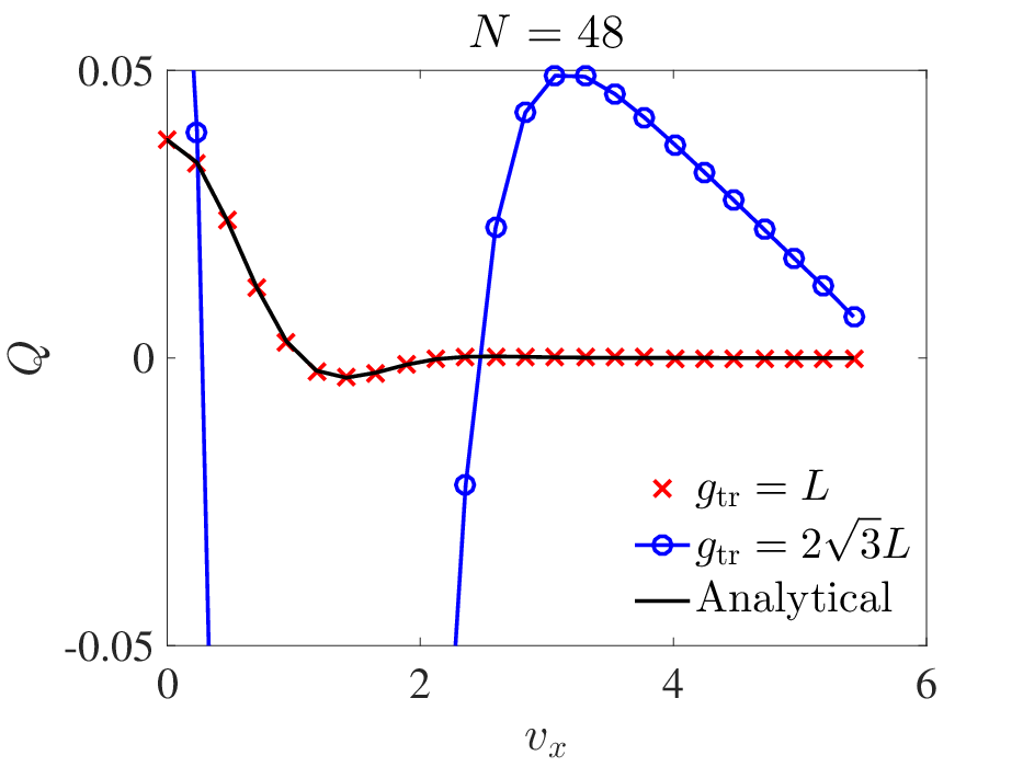
In Fig. 1 (left) we plot slices of the collision operator on a linear scale with $g_{\text{tr}}=L$ and $g_{\text{tr}}=2\sqrt{3}L$. For these results we used $N=48$ discretization points in each velocity direction. The result with $g_{\text{tr}}=L$ agrees well with the analytical formula for $Q$ obtained using (4) and (17). However, the result with $g_{\text{tr}}=2\sqrt{3}L$ is far from being correct, which suggests that in their numerical simulations Gamba and Tharkabhushanam actually used a significantly smaller value of $g_{\text{tr}}$, although they do not state which value they chose.

The reason for the lack of agreement with $g_{\text{tr}}=2\sqrt{3}L$ is that the integral (13) for $\widehat{Q}^{\text{tr}}$ is numerically computed using values of $\widehat{f}$ and $\widehat{G}^{\text{tr}}$ on a grid with spacing

This grid spacing is determined by the standard discretization of the Fourier transform. With this grid spacing there can be significant error in the numerical computation of the integral, since as we see from (15) and (16), the kernel, $\widehat{G}^{\text{tr}}$, oscillates on a length scale of approximately $2\pi/g_{\text{tr}}$. Increasing the number of discretization points, $N$, in each velocity dimension does not change $\Delta\xi$. On the other hand, the agreement is much better with $g_{\text{tr}}=L$, since the frequency of oscillation of $\widehat{G}^{\text{tr}}$ is approximately half that of the sampling frequency, $\Delta\xi=\pi/g_{\text{tr}}$, in accord with the Nyquist-Shannon sampling theorem.

Because we are interested in computing the low-probabilty tails of the velocity pdf, it is important to determine how the choice of $g_{\text{tr}}$ affects the relative error in the numerically computed values of collision operator at large speeds, $v=|\mathbf{v}|$. To start investigating this question, in Fig. 1 (right) we plot slices of the absolute value of the collision operator on a logarithmic scale. We note that the cusps evident in the log-scale plots occur where $Q$ changes sign. The three numerical results were obtained using $g_{\text{tr}}=5.66$ but with different choices for $N$ and for the grid spacing $\Delta\xi=\pi/L$ used in the numerical computation of the integral (13). The red line with crosses and the green line with diamonds shows the results with $N=56$ and $N=112$, respectively. In both cases we choose $L=g_{\text{tr}}=5.66$, which results in $\Delta\xi=0.56$. We see from these results that doubling $N$ increases the accuracy of the computation by about an order of magnitude. The reason is that $\widehat{G}^{\text{tr}}$ decays slowly as $|\boldsymbol{\xi}|\to\infty$ and increasing $N$ increases the size of the domain of integration in frequency space. The blue curve with circles shows the result with $N=112$ and $L=2g_{\text{tr}}=11.32$, so that $\Delta\xi=0.28$. Comparing the red and blue curves, we see that halving $\Delta\xi$ increases the accuracy of the computation by about two orders of magnitude. The reason is the smaller grid spacing better captures the oscillations of $\widehat{G}^{\text{tr}}$.

One of our main goals in this paper is to fix $L$ and investigate how small we can choose both $g_{\text{tr}}$ and $N$ so as to accurately compute the velocity pdf down to a desired probability level. If we let $Q^{\text{NC}}$ denote the collision operator obtained by numerically computating of $Q^{\text{tr}}$, then the total error,

is bounded by

The first term on the right hand side of (20) is the error inherent in the truncation of the collision operator, and the second term is the error in the numerical computation of the truncated operator. Since in practice, we have limited computational resources the choice of $g_{\text{tr}}$ involves a trade off between these two sources of error.

In this section, we first review a theorem of Cercignani et al. [27] on the convergence of $Q^{\text{tr}}$ to $Q$ as $g_{\text{tr}}\to\infty$. However, since this theorem does not include an error bound, it is of limited utility for numerical computation. Then, we derive an upper bound on the pointwise error between $Q$ and $Q^{\text{tr}}$, assuming that both operators are computed exactly. This bound provides some additional theoretical justification for the spectral-Lagrangian method. In Section 6, we will use this upper bound to guide the choice of $g_{\text{tr}}$ in numerical computations.

Cercignani et al. [27] use the truncated collision operator in a proof of an existence and uniqueness theorem for solutions of the homogeneous Boltzmann equation. In their proof they consider the initial value problem,

where $Q^{M}=Q^{\text{tr}}$ with $g_{\text{tr}}=M<\infty$. They show that (21) has a unique nonnegative solution $f^{M}\in C^{1}([0,T],L^{1}(\mathbb{R}^{3}))$ for all $T>0$, provided that $f_{0}\in L^{1}(\mathbb{R}^{3})$ is nonnegative. In addition, they show that the total mass, momentum, and energy are conserved by (21). Applying the Dunford-Pettis theorem to the set $\{f^{M}\}$ in $C^{1}([0,T],L^{1}(\mathbb{R}^{3}))$, they extract a weakly convergent subsequence $f^{n}\rightharpoonup f$, with $f\in C^{1}([0,T],L^{1}(\mathbb{R}^{3}))$ nonnegative, and prove that $Q^{M_{n}}(f^{n},f^{n})\rightharpoonup Q(f,f)$. Here, by weak convergence we mean convergence of the sequence obtained after integration against a test function in $L^{\infty}(\mathbb{R}^{3})$.

To assess the trade off discussed at the end of Section 3, we now present an upper bound for the error inherent in the truncation of $Q$, i.e., for the first term on the right hand side of (20). Specifically, we let

where $Q=Q(f,f)$ and $Q^{\text{tr}}=Q^{\text{tr}}(f,f)$. Since these two collision operators are defined in terms of the same velocity pdf, $f$, this result has a different character than that of Cercignani.

To obtain this result, rather than assuming that the support of $f$ is compact, we instead assume that $f$ is bounded above by a Maxwellian pdf. For Maxwell-type collisions between particles of the same type, Bobylev and Gamba [33] proved that, if the initial condition satisfies $f_{0}(\boldsymbol{v})\leq c_{0}\,e^{-k_{0}v^{2}}$, then there are constants $c\geq c_{0}$ and $k\leq k_{0}$ so that $f(\boldsymbol{v},t)\leq c\,e^{-kv^{2}}$ for all $t>0$. Moreover, they provide formulae for $c$ and $k$ in terms of $c_{0}$, $k_{0}$, and the initial pdf $f_{0}$. Gamba et al. [34] proved similar results for other interparticle collision kernels. Consequently, the assumptions we make in the following theorem and in its corollary are reasonable.

Since $Q$ is the rate of change of $f$, we expect $Q(\mathbf{v})$ to be on the order of $c\exp(-kv^{2})$ or less. Therefore, we can regard the error, $\mathcal{E}_{\operatorname{rel}}$, in (24) as a measure of the relative error between $Q$ and $Q^{\text{tr}}$. Note that since $Q$ has zeros, we have defined this error to be relative to a Maxwellian pdf rather than to $Q$. The upper bound, $\mathcal{E}_{\operatorname{rel}}$, in (24) can be used to guide the choice of $g_{\text{tr}}$ in numerical simulations by ensuring that $\mathcal{E}_{\operatorname{rel}}(g_{\operatorname{tr}},{v})<10^{-m}$ for a desired value of $m$, over a given range of values for $v$.

Equation (34) yields the following simple strategy for choosing the parameter, $g_{\operatorname{tr}}$, in numerical computations of the low-probability tails. Specifically, to guarantee $Q^{\operatorname{tr}}$ is an accurate approximation to $Q$ at $\mathbf{v}$, we should choose $g_{\operatorname{tr}}$ to be slightly larger than $v$. As we will see in Section 6, exactly how much larger depends on the values of $c$ and $k$ and the desired degree of accuracy.

We implement Gamba’s method as in [13, 28]. The computational grids in velocity and Fourier space are defined in terms of a maximum speed, $L$, and the number of grid points, $N$, in each dimension. Unless otherwise noted, we use $L=10$. We represent the velocity pdf on a domain $[-L,L]^{3}\in\mathbb{R}^{3}$ using a regular grid, $v_{k}=-L+k\Delta v$, in each velocity dimension, where $\Delta v=2L/N$. The corresponding domain in Fourier space is $[-\zeta_{\rm max},\zeta_{\rm max}]^{3}$, where $\zeta_{\rm max}=N\pi/2L$, with grid points, $\zeta_{m}=-\zeta_{\rm max}+m\Delta\zeta$, where $\Delta\zeta=\pi/L$. We calculate the integral (13) using the trapezoid rule, which—like the discrete Fourier transform—is spectrally accurate for functions that decay rapidly at the boundary of the computation domain [36]. In addition, for the numerical results in Sections 6.1–6.4 below we enforce conservation of the density, momentum, and energy using the Lagrangian projection method of [13], which amounts to projecting the collision operator onto a linear subspace in $L^{2}(\mathbb{R}^{3})$. However, we found that the results in these subsections are visually indistinguishable from those we obtained without the application of the Lagrangian projection method. Because of the large cost of computing the collision operator, we use a multistep method to solve the system of differential equations corresponding to (4), which allows us to take larger time steps resulting in a fewer total number of function evaluations. Specifically, we used the fourth order Adams-Bashforth method [37]

where $f_{i}(\boldsymbol{v})=f(t_{i},\boldsymbol{v})$ and $Q_{i}=Q^{\operatorname{tr}}(f_{i},f_{i})$. To initialize this multistep method we used the fourth order Runge Kutta method to compute the solutions at the first four time steps.

In this section we present the results of the numerical simulations we performed to test the limits of the spectral-Lagrangian method. We show results for the following choices of initial condition: a Maxwellian, the spherically symmetric, analytical solution of Bobylev, Krook and Wu [30, 31], a cylindrically symmetric modification of the BKW initial condition, and two mixtures of Maxwellians. We study the convergence of the numerically computed truncated collision operator, $Q^{\operatorname{NC}}$, to the collision operator, $Q$, validate the bound we obtained for the relative error between $Q^{\operatorname{tr}}$ and $Q$, and compute the evolution of the velocity pdf to the equilibrium Maxwellian distribution. In these simulations our focus is on the accuracy with which the velocity pdfs can be computed in the low probability tails. Finally, we employ a simple model of a plasma to study the evolution of the velocity pdf of the electrons under the influence of an electron gun source, electron-electron collisions, and loss into a boundary sheath layer.

The simulations were performed on a 2.0 GHz Intel Xeon processor with 2 CPU’s and 14 cores per CPU. The total simulation time (number of cores $\times$ time per core) for a single computation of the collision operator ranged from 24 seconds for $N=24$ to 4.5 hours for $N=72$, and scaled according to the theoretical $\mathcal{O}(N^{6})$ cost.

References

- [1] B. Gustavsson, T. Sergienko, I. Häggström, F. Honary, T. Aso, Simulation of high energy tail of electron distribution function, Adv. Polar Upper Atmos. Res. 18 (2004) 1–9.
- [2] J. Allen, On the applicability of the Druyvesteyn method of measuring electron energy distributions, Journal of Physics D: Applied Physics 11 (3) (1978) L35.
- [3] J. V. Dicarlo, M. J. Kushner, Solving the spatially dependent Boltzmann’s equation for the electron velocity distribution using flux corrected transport, J. Appl. Phys. 66 (12) (1989) 5763–5774.
- [4] T. Sheridan, M. Goeckner, J. Goree, Electron velocity distribution functions in a sputtering magnetron discharge for the E B direction, Journal of Vacuum Science & Technology A: Vacuum, Surfaces, and Films 16 (4) (1998) 2173–2176.
- [5] C. Sozzi, E. De La Luna, D. Farina, J. Fessey, L. Figini et al., Measurement of electron velocity distribution function, AIP Conference Proceedings 988 (73) (2008) 73–80.
- [6] W. Tan, Langmuir probe measurement of electron temperature in a Druyvesteyn electron plasma, Journal of Physics D: Applied Physics 6 (10) (1973) 1206.
- [7] J. Poulose, M. Goeckner, S. Shannon, D. Coumou, L. Overzet, Driving frequency fluctuations in pulsed capacitively coupled plasmas, The European Physical Journal D 71 (9) (2017) 242.
- [8] A. G. Bird, Molecular Gas Dynamics, Clarendon Press, Oxford, 1994.
- [9] K. Nanbu, Direct simulation scheme derived from the Boltzmann equation. I. Monocomponent gases, J. Phys. Soc. Japan 52 (1983) 2042–2049.
- [10] W. Wagner, A convergence proof for Bird’s direct simulation Monte Carlo method for the Boltzmann equation, Journal of Statistical Physics 66 (3) (1992) 1011–1044.
- [11] I. M. Gamba, S. Rjasanow, W. Wagner, Direct simulation of the uniformly heated granular Boltzmann equation, Mathematical and Computer Modeling 42 (5-6) (2005) 683–700.
- [12] S. Rjasanow, W. Wagner, Stochastic Numerics for the Boltzmann Equation, Springer, Berlin, 2005.
- [13] I. M. Gamba, S. H. Tharkabhushanam, Spectral-Lagrangian methods for collisional models of non-equilibrium statistical states, Journal of Computational Physics 228 (2009) 2012–2036.
- [14] C. Mouhot, L. Pareschi, Fast algorithm for computing the Boltzmann collision operator, Math. Comp. 75 (256) (2006) 1833–1852.
- [15] L. Pareschi, B. Perthame, A Fourier spectral method for homogeneous Boltzmann equations, Transport Theory and Statistical Physics 25 (3-5) (1996) 369–382.
- [16] L. Pareschi, G. Russo, Numerical solution of the Boltzmann equation. I. Spectrally accurate approximation of the collision operator, SIAM J. Numerical Anal. 37 (4) (2000) 1217–1245.
- [17] I. M. Gamba, J. R. Haack, A conservative spectral method for the Boltzmann equation with anisotropic scattering and the grazing collisions limit, Journal of Computational Physics 270 (2014) 40–57.
- [18] I. M. Gamba, J. R. Haack, C. D. Hauck, J. Hu, A fast spectral method for the Boltzmann collision operator with general collision kernels, SIAM Journal on Scientific Computing 39 (4) (2017) B658–B674.
- [19] I. M. Gamba, S. H. Tharkabhushanam, Shock and boundary structure formation by spectral-Lagrangian methods for the inhomogenerous Boltzmann transport equation, Journal of Computational Mathematics 28 (2010) 430–460.
- [20] J. R. Haack, I. M. Gamba, High performance computing with a conservative spectral Boltzmann solver, in: AIP Conference Proceedings, Vol. 1501, AIP, 2012, pp. 334–341.
- [21] A. Munafò, J. R. Haack, I. M. Gamba, T. E. Magin, A spectral-Lagrangian Boltzmann solver for a multi-energy level gas, Journal of Computational Physics 264 (2014) 152–176.
- [22] I. M. Gamba, S. Rjasanow, Galerkin-Petrov approach for the Boltzmann equation, Journal of Computational Physics 366 (2018) 341–365.
- [23] E. Fonn, P. Grohs, R. Hiptmair, Hyperbolic cross approximation for the spatially homogeneous Boltzmann equation, IMA Journal of Numerical Analysis 35 (4) (2014) 1533–1567.
- [24] Z. Cai, Y. Fan, L. Ying, An entropic Fourier method for the Boltzmann equation, SIAM Journal on Scientific Computing 40 (5) (2018) A2858–A2882.
- [25] I. M. Gamba, J. R. Haack, J. Hu, A fast conservative spectral solver for the nonlinear Boltzmann collision operator, in: AIP Conference Proceedings, Vol. 1628, AIP, 2014, pp. 1003–1008.
- [26] R. Alonso, I. Gamba, S. Tharkabhushanam, Convergence and error estimates for the Lagrangian-based conservative spectral method for Boltzmann equations, SIAM Journal on Numerical Analysis 56 (6) (2018) 3534–3579.
- [27] C. Cercignani, R. Illner, M. Pulvirenti, The mathematical theory of dilute gases, Vol. 106, Springer Science & Business Media, 2013.
- [28] J. Haack, A hybrid OpenMP and MPI implementation of a conservative spectral method for the Boltzmann equation, ArXiv e-printshttp://adsabs.harvard.edu/abs/2013arXiv1301.4195H (Jan 2013).
- [29] J. Duistermaat, J. Kolk, Distributions: Theory and Applications, Springer, New York, 2010.
- [30] A. Bobylev, Exact solutions of the Boltzmann equation, in: Akademiia Nauk SSSR Doklady, Vol. 225, 1975, pp. 1296–1299.
- [31] K. Max, W. T. Tsun, Formation of Maxwellian tails, Physical Review Letters 36 (1976) 1107–1109.
- [32] A. V. Bobylev, S. Rjasanow, Difference scheme for the Boltzmann equation based on the fast Fourier transform, European Journal of Mechanics - B/Fluids 16 (2) (1997) 869–887.
- [33] A. Bobylev, I. Gamba, Upper Maxwellian bounds for the Boltzmann equation with pseudo-Maxwell molecules, Kinet. Relat. Models 10 (3) (2017) 573–585.
- [34] I. Gamba, V. Panferov, C. Villani, Upper Maxwellian bounds for the spatially homogeneous Boltzmann equation, Arch. Rat. Mech. Anal. 194 (2009).
- [35] N. Bleistein, R. A. Handelsman, Asymptotic expansions of integrals, Courier Corporation, 1986.
- [36] L. N. Trefethen, Spectral Methods in MATLAB, SIAM, 2000.
- [37] D. R. Kincaid, E. W. Cheney, Numerical Analysis: Mathematics of Scientific Computing, Wadsworth, Inc, Belmont, California, 1991.