On the price of explainability for some clustering problems
Abstract
The price of explainability for a clustering task can be defined as the unavoidable loss, in terms of the objective function, if we force the final partition to be explainable.
Here, we study this price for the following clustering problems: -means, -medians, -centers and maximum-spacing. We provide upper and lower bounds for a natural model where explainability is achieved via decision trees. For the -means and -medians problems our upper bounds improve those obtained by [Moshkovitz et. al, ICML 20] for low dimensions.
Another contribution is a simple and efficient algorithm for building explainable clusterings for the -means problem. We provide empirical evidence that its performance is better than the current state of the art for decision-tree based explainable clustering.
1 Introduction
Machine learning models and algorithms have been used in a number of systems that take decisions that affect our lives. Thus, explainable methods are desirable so that people are able to have a better understanding of their behavior, which allows for comfortable use of these systems or, eventually, the questioning of their applicability.
Although most of the work on the field of explainable machine learning has been focusing on supervised learning [31, 23, 34], there has recently been some effort to devise explainable methods for unsupervised learning tasks, in particular, for clustering [26, 6]. We investigate the framework discussed by [26], where an explainable clustering is given by a partition, induced by the leaves of a decision tree, that optimizes some predefined objective function.
Figure 1 shows a clustering with three groups induced by a decision tree with leaves. As an example, the blue cluster can be explained as the set of points that satisfy Feature 1 and Feature 2 . Simple explanations as this one are usually not available for the partitions produced by popular methods such as the Lloyd’s algorithm for the -means problem.
![[Uncaptioned image]](2101.01576v2/Exp-Clustering.jpg)
In order to achieve explainability, one may be forced to accept some loss in terms of the quality of the chosen objective function (e.g. sum of squared distances). In this sense, explainability has its price. [26] presents theoretical bounds on this price for the -medians and the -means objective functions.
Here, we expand on their work by presenting new bounds for these objectives and also providing nearly tight bounds for two other goals that arise in relevant clustering problems, namely, the -centers and the maximum-spacing problems. We note that the objective for the latter is the one optimized by the widely known Single-Linkage method, employed for hierarchical clustering. We also give a more practice-oriented contribution by devising and evaluating a simple and efficient algorithm for building explainable clusterings for the -means problem.
1.1 Problem definition
Let be a set of points in . We say that a decision tree is standard if each internal node is associated with a test (cut), specified by a coordinate and a real value , that partitions the points in that reach into two sets: those having the coordinate smaller than or equal to and those having it larger than . The leaves of a standard decision tree induce a partition of into axis-aligned boxes and, naturally, a partition of into clusters.
Let be an integer. The clustering problems considered here consist of finding a partition of into groups, among those that can be induced by a standard decision tree with leaves, that optimizes a given objective function. For -means, -medians and -centers, in addition to the partition, a representative for each group must also be output.
For the -means problem the objective (cost function) to be minimized is the Sum of the Squared Euclidean Distances (SSED) between each point and the representative of the cluster where lies. Mathematically, the cost (SSED) of a partition for is given by
The -medians and the -centers problems are also minimization problems. For the former, the cost of a partition is given by
while for the latter it is given by
The maximum-spacing problem is a maximization problem for which the objective to be maximized is the spacing of a partition , defined as
We note that an optimal solution of the unrestricted version of any of these problems, in which the decision tree constraint is not enforced, might be a partition that is hard to explain in terms of the input features. Thus, the motivation for using decision trees.
Along the lines of [26], we define the price of explainability for a clustering problem , with a minimization objective function, as
where runs over all instances of ; is the cost of an optimal explainable clustering (via standard decision trees) for instance and is the cost of an optimal unrestricted clustering for . If has a maximization objective function, then is defined as
1.2 Our Contributions
We provide bounds on the price of explainability as a function of the parameters and for the aforementioned objective functions. These objectives cover a spectrum that includes both intra- and inter-clustering criteria as well as worst-case and average-case measures.
First, we address the -centers problem. We show that
and that is . Our bounds are tight, up to constant factors, when is a constant. For an arbitrary , there is only a polylogarithmic gap in between the upper and the lower bounds. The magnitude of this gap is exponentially smaller than that of these bounds.
For the -medians it is known that the price of explainability is and [26]. We contribute to the state of the art by showing that is also an upper bound – an exponential improvement for constant dimensions. The upper bound follows from an interesting connection with the literature of binary searching in the presence of non-uniform testing costs [8, 20].
For the -means problem, we also improve, for low dimensions, the bound from [26] since we prove that is . Still, for the -means problem, we also give a more practice-oriented contribution by devising and evaluating a simple and efficient greedy algorithm. Our method outperformed the IMM method from [26] on an empirical study involving 10 real datasets. It should be noticed that IMM is a strong baseline since it got the best results against 5 other competitors on the same datasets according to [12, 15].
Finally, for maximum-spacing we provide a tight bound by showing that the price of explainability is . The lower bound is particularly interesting since it shows that this objective function is bad for guiding explainable clustering, losing much more than the other considered objectives in the worst-case.
To derive our upper bounds, we analyze polynomial-time algorithms that start with an optimal -clustering and transform it into an explainable one. The unrestricted versions of all the problems considered here, except for the maximum-spacing problem, are NP-Hard [24, 2]. However, all of them admit polynomial-time algorithms with constant approximation [35, 18] and, hence, if we start with the partitions given by them, instead of the optimal ones, we obtain efficient algorithms with provable approximation guarantees. These guarantees are exactly the upper bounds that we prove on the price of explainability.
We believe that our results are helpful for the construction of explainable clustering solutions as well as for guiding the choice of an objective function when explainability is required.
1.3 Related Work
Our research is inspired by the recent work of [26], where they propose an algorithm, namely IMM, for building explainable clusterings, via standard decision trees, for both the -means and the -medians problems. At each node IMM selects the cut that minimizes the number of points separated from their representatives in a reference clustering. Our approach for these problems, while similar, uses a significantly different strategy to build the final decision tree, based on trees that look at a single dimension of the data. Moreover, as mentioned before, our algorithms provide better upper bounds for low dimensions.
Decision trees have long been associated to hierarchical agglomerative clustering (HAC), which produces a hierarchy of clusters that is usually represented by a dendrogram. Examples of models that explicitly use decision trees for HAC include [13, 9, 7, 4]. To our knowledge, the use of decision trees for non-hierarchical clustering was first suggested in [21], in which a standard classification tree is used to identify dense and sparse regions of data. In [14], unsupervised binary trees are also used to create interpretable clusters. More recently, an approach was presented in [6] using optimal classification trees [5], which are built in a single step by solving a mixed-integer optimization problem. For numerical databases, [22] presents a decision approach that decides on a split based on both the compactness of clusters and the separation between them.
The regions of space defined by decision-tree clustering will be hyper-rectangles (some of them may also be half-spaces if the overall region of interest is unbounded). Other approaches towards building hyper-rectangular clusters can be found in [29], with a generative model, and [11], with a discriminative one. Both models allow for probabilistic (soft) clustering, and [11] allows for incorporating previous knowledge to the model, but neither one guarantees that the resulting clusters can be represented by decision trees.
The main reason for using a (short) decision tree to build clusters is that the results of such algorithms are easily interpretable. Other avenues towards interpretable clustering have been explored in recent years. The technique presented in [30] is based on the information-theoretic concept of minimum description length. In [33], a tunable parameter (the fraction of elements in a cluster that share the same feature value) leverages the tradeoff between clustering performance and interpretability. The same tradeoff is explored in [15] by relaxing the requirement from [26] that the explainable clustering should be induced by a tree with no more than leafs. In [17], a feature selection model from [16] is used for clustering interpretation in the field of wealth management compliance. [19] uses a two-step approach, rewriting -means clustering models as neural networks and applying to these networks techniques for interpreting supervised learning models. More information regarding explainable clustering may be found in [10, 3].
Of all the works mentioned in this section, only [26] presents approximation guarantees with respect to the optimal unrestricted (i.e., potentially uninterpretable) solution. Two algorithms from [33] also have an approximation guarantee, but with respect to the optimal restricted (interpretable) solution, and the definition of interpretability in that work is quite different than ours (interpretable clusters are therein defined as those in which a given proportion of points share the same value for a predefined feature of interest).
Explainability and interpretability are topics of growing interest in the machine learning community [31, 23, 1, 32, 27, 25]. While there has been some focus on what [26] calls post-modeling explainability, or the ability to explain the output of a black-box model [31, 23, 19], the practice has also been criticized in contrast with pre-modelling explainability, or the use of interpretable models to begin with [32]. Our present work and [26] may be considered a middle-of-the-road approach, as the end result is a fully interpretable model (instead of, for instance, a model for locally interpreting the original model, or for explaining individual predictions) based on the output from a potentially black-box model.
2 On the Price of Explainability for the -centers problem
In this section we address the -centers problem. We first present a lower bound by constructing an instance for which the price of explainability is high.
2.1 Lower Bound
Let be a positive integer whose exact value will be defined later in the analysis and let be the largest integer for which . Note that . Moreover, let .
Our instance has points. We first discuss how to construct the points, referred as centers, that will be set as representatives in an unrestricted -clustering for that has a low cost. The first centers will be obtained from the representation of the numbers in base while the remaining centers will be located sufficiently far from the others so that they will be isolated in the low-cost -clustering for . Let be the first centers.
For a number let be its representation in base . For , the value of the -th component of center is obtained by applying times a circular shift on . The values of the remaining components of are obtained by copying the first values times so that if .
As an example, if , and then . In fact, since we have that ; and . The values of are obtained by repeating the first 3 values.
The following observation is useful for our analysis.
Fact 1.
For every , the values of the -th coordinate of the first centers are a permutation of the integers .
The remaining centers, as mentioned above, should be far from each other and also far away from the first centers. We can achieve that by setting for all , where is the unit vector in .
The next lemma gives a lower bound on the distance between any two centers.
Lemma 1.
For any two centers and ,
Proof.
If one of the two centers is not among the first centers the result clearly holds. Thus, we assume that .
It is enough to show that there is for which . In fact, if this inequality holds for some then for each that is congruent to modulo . Since there are of them, due to our construction, we get the desired bound.
Let and be the representations of and in base , respectively. Let be such that is maximum.
Thus, the difference between and in the coordinate is at least
where the last inequality holds because and . ∎
Now, we define the remaining points of instance .
For each of the first centers we create associated points: . For , the point is identical to in all coordinates but on the -th one, in which its value is . Similarly, the point is identical to in all coordinates but in the -th one, in which its value is . By considering the -clustering for where the representatives are the centers and each point lies in the group of , we obtain the following proposition.
Proposition 1.
There exists an unrestricted -clustering for instance with cost .
Now we analyse the cost of an optimal explainable clustering for . The following proposition is a simple consequence of Fact 1.
Proposition 2.
Let be a cut that separates at least two points from the set that includes the first centers and its associated points. Then, separates one point from its associated center.
Proof.
Since separates at least two points from then .
If , then separates the center that has the -th coordinate equal to 0 from its associated point that has coordinate equal to . If , then separates the center that has the -th coordinate equal to 0 from its associated point that has coordinate equal to . Let be an integer that satisfies and such that . If (resp. ), separates the center that has the -th coordinate equal to (resp. ) from its associated point with -th coordinate equal to (resp. ).
Note that the existence of centers with the aforementioned values for coordinate is guaranteed by Fact 1. ∎
Lemma 2.
Any explainable -clustering for instance has cost at least .
Proof.
Let be an explainable -clustering for instance . It is enough to show that there is a cluster that contains two points, say and , for which
In fact, in this case, due to the triangle inequality, for any choice of the representative for , either or will be at distance at least from it.
If two centers lie in the same cluster of then it follows from Lemma 1 that their distance is at least .
On the other hand, if every center lies on a different cluster in then let be the point that was separated from its center, say , by a cut that satisfies the condition of Proposition 2. Then, lies in the same cluster of , for some . From the triangle inequality we have that
Hence, . ∎
By putting together Proposition 1 and Lemma 2 and, then, optimizing the value of we obtain the following theorem.
Theorem 1.
The price of explainability for the -centers problem satisfies
Proof.
Proposition 1 assures the existence of a -clustering of cost for instance . Let be an explainable clustering for and recall that . It follows from the previous lemma that
Since we have
Thus,
Now we set if and , otherwise. Since we have that for both cases and, hence,
By replacing in the previous equation according to each of the cases we obtain the desired result. ∎
2.2 Upper bound
In this section we show that the price of explainability for the -center problem is . Note that, for constant , the upper bound matches the lower bound given by Theorem 1.
To obtain the upper bound we analyze the cost of the explainable clustering induced by the decision tree built by the algorithm presented in Algorithm 1.
The algorithm has access to the set of representatives of an optimal -clustering for . These representatives are used as reference centers for the points in , that is, the reference center of a point is the representative of ’s group in .
Let and be, respectively, the subset of points in and the set of reference centers that reach a given node . To split , as long as it is possible, the algorithm applies an axis-aligned cut that does not separate any point from its reference center. This type of cut is referred as a clean cut with respect to . When there is no such cut available for , the algorithm partitions the bounding box of the points in into axis-aligned boxes of the same dimensions by using a decision tree that emulates a grid. By the bounding box of we mean the smallest box (hyper-rectangle) with axis-aligned sides that includes the points in .
Theorem 2.
The price of explainability for -centers is .
Proof.
We argue that for each leaf of the tree built by Ex-kCenter(), the maximum distance between a point in and its representative is , where is the cost of the optimal unrestricted clustering.
We split the proof into two cases. The first case addresses the scenario in which only clean cuts are used in the path from the root of to the leaf . The second case addresses the remaining scenarios.
Case 1. In this case all points that reach lie in the same cluster of the optimal unrestricted -clustering . Thus, the maximum distance from a point in to the single reference center in is upper bounded by .
Case 2. Let be the first node in the path from the root to for which a clean cut is not available. Moreover, let be the set of points that reach and let , that is, the number of reference centers that reach . In this case the algorithm splits the bounding box for into boxes of dimensions
where is the difference between the maximum and minimum values of the -th coordinate among points in .
The maximum distance between a point in and its representative can be upper bounded by the length of the diagonal of the axis-aligned box corresponding to . Let be such that . Then, the length of the diagonal is upper bounded by .
Thus, it suffices to show that . Let be the reference centers that reach node . In addition, let be a point in with reference center and such that is maximum, among the points in with reference center . Then, we must have
for otherwise there would be a clean cut , with , where and . Hence, for some point , . Since we get that . ∎
3 Improved Bounds on -medians for low dimensions
We show that the price of explainability for -medians is , which improves the bound from [26] when .
As in the previous section we use an optimal unrestricted -clustering for as a guide for building an explainable clustering. Again, by the reference center of a point we mean its representative in .
We need some additional notation. For a decision tree and a node , let be the -dimensional vector whose -th coordinate is given by the difference between the maximum and the minimum values of coordinate among the reference centers that reach . Let be the number of points that reach and are separated from their reference centers by the cut employed in . Note that a point can only contribute to if both and its reference center reach . Finally, we use to denote the cost of the optimal unrestricted clustering .
The following lemma from [26], expressed in our notation, will be useful.
Lemma 3.
[26] Let be an optimal unrestricted -clustering for and let be a decision tree for in which each representative of lies in a distinct leaf. Then, the clustering induced by satisfies
| (1) |
In order to obtain a low-cost explainable clustering we focus on finding a decision tree for which the rightmost term of the above inequality is small. This is the approach taken by IMM [26], a greedy strategy that at each node selects the cut that yields the minimum possible value for .
Although we follow the same approach, our strategy for building the tree is significantly different. In order to explain it, we first rewrite the rightmost term of (1):
| (2) |
Motivated by Lemma 3 and the above identity, our strategy constructs decision trees , where is built with the aim of minimizing
| (3) |
ignoring the impact on the coordinates .
Next, it constructs a decision tree for by picking nodes from these trees. More precisely, to split a node of the strategy first selects a coordinate for which is maximum. Next, it applies the cut that is associated with the node in which is the least common ancestor (LCA) of the set of reference centers that reach .
In the pseudo-code presented in Algorithm 2, is a subset of the set of representatives of . Moreover, is a subset of the points in . The procedure is called, initially, with and .
To fully specify the algorithm we need to explain how the decision trees are built. Let be the reference centers sorted by coordinate , that is, for . Moreover, let be the cut that separates the points in with the -th coordinate smaller than or equal to from the remaining ones.
For , let be the family of binary decision trees with internal nodes and leaves defined as follows:
- (i)
if , then has a single tree and this tree contains only one node.
- (ii)
if , then consists of all the decision trees with the following structure: the root of is identified by a number and associated with the cut ; one child of the root of is a tree in the family while the other is a tree in .
For our analysis, in the next sections, it will be convenient to view as the family of binary search trees for the numbers in the set .
Let be the number of points in that are separated from their centers by cut . For every tree we define as
where is the diameter of the node identified by in .
The tree is, then, defined as
The motivation for minimizing is that for every tree , is an upper bound on (3), that is,
To see that, let be the integer identified with the node . By definition . Moreover, we have because only accounts the points that are separated from their reference centers among those that reach , while accounts all the points in regardless of whether they reach or not.
We discuss how to construct efficiently. Let if , and let if . Hence, . The following relation holds for all :
| (4) |
Thus, given a set of reference centers and the values ’s, can be computed in time by solving equation (4), for and , via standard dynamic programming techniques.
3.1 Approximation Analysis: Overview
We prove that the cost of the clustering induced by is . To reach this goal, we first show that
| (5) |
The proof of this bound relies on the fact that can be seen as a binary search tree with non-uniform probing costs. We use properties of this kind of tree, in particular the one proved in [8] about its competitive ratio.
Let
be the contribution of coordinate to , where is the reference center of . Our second step consists of showing that
| (6) |
Roughly speaking, the proof of this bound consists of projecting the points of and the reference centers onto the axis and then counting the number of times the interval appears in the segments that connect points in to their reference centers. This is exactly the same line of reasoning employed to prove Lemma 6 from the supplementary version of [26].
At this point, from the two previous inequalities, we obtain
| (7) |
Finally, we prove that a factor of is incurred when we build the tree from the nodes of the trees :
| (8) |
From (7), (8) and the identity , we obtain
This together with Lemma 3 allows us to establish the main theorem of this section.
Theorem 3.
The price of explainability for -medians is .
3.2 Approximation Analysis: Proofs
We start with the proof of inequality (5).
Lemma 4.
The tree satisfies
Proof.
Let be a tree in . By construction, the set of centers that reach the node in identified by is a contiguous subsequence of . Let and be, respectively, the first and the last indexes of the centers of this subsequence. Thus,
| (9) |
We can show that the right-hand side of the above equation satisfies
| (10) |
where is the set of nodes that are ancestors (including ) of the node identified by in .
To see that, fix . The term contributes the left-hand side of (10) if the centers and reach the node in . This happens if and only if is an ancestor of the node identified by in .
Now, we use Theorem 4.5 from [8]. It states that for any vector of non-negative real numbers there exists a binary search tree having nodes, with each of them associated with a number in , that satisfies
for every node of .
Inequality (6) is formalized in the next lemma.
Lemma 5.
Let be the contribution of the coordinate for the cost of an optimal unrestricted clustering . Then,
| (11) |
where is the reference center of .
Proof.
Let be the reference centers sorted by increasing order of coordinate . Recall that . For every , let .
Fix . If then either or is included in the real interval with endpoints and . Thus, we have that
By adding the above inequality for all we conclude that the number of times that contributes to the right-hand side, for every , is exactly the number of times that separates a point from its reference center . This number is exactly . ∎
Finally, we present the proof of inequality (8).
Lemma 6.
Let be the decision tree built by Algorithm 2. Then,
Proof.
For a node , let be the (possibly empty) set of nodes in the tree that correspond to , that is, the nodes that use the cut associated with the node from . We have
| (12) |
Moreover, we have that
| (13) | |||
| (14) |
where the first inequality in (13) holds because is the coordinate for which the diameter of is maximum and the inequality (14) holds because the set of centers in is a subset of the set of centers that reach the node identified by in .
Claim 1.
For a node , let be the set of points that reach in . Then, for every , with .
Proof.
Let be the least common ancestor of and in . If then the cut associated with splits into two disjoint regions, one of them containing and the other containing so that and are disjoint.
If let us assume w.l.o.g. that . In this case, the cut , associated with , splits into two regions, one of them containing all the reference centers that reach . These centers are contained in the set of reference centers of one of the children of in and, hence, the LCA in of the set of centers that reach is not , that is, . This contradiction shows that this case cannot occur. ∎
Hence, it follows from (12) that
4 The -means problem
4.1 Improved bounds for low dimensions
The result we obtained for the -medians problem can be extended to the -means problem:
Theorem 4.
The price of explainability for -means is .
From an algorithmic perspective, in order to establish the theorem, we only need to replace the definition of for a tree in with
Note that the only difference is the replacement of with . As a consequence, for the -means problem, the tree is defined as the tree in for which is minimum. It can also be constructed via dynamic programming. Theorem 4 can be proved by using arguments similar to those employed to bound the price of explainability for -medians. The following inequalities are, respectively, counterparts of the inequalities (1), (5), (6) and (8):
| (15) |
| (16) |
| (17) |
| (18) |
From the three last inequalities and the identity , we obtain
This together with the inequality (15) allows us to establish Theorem 4.
Inequality (15) is proved in [26]. The validity of inequalites (17) and (18) can be established by using exactly the same arguments employed to prove their counterparts. More specifically, the proof of Lemma 5 can be used for the former while the proof of Lemma 6 can be used for the latter.
The inequality (16) incurs an extra factor of with respect to its counterpart. In order to prove this inequality, we apply the arguments of the proof of Lemma 4. The only required adaptation consists of replacing Equation (9) with the inequality
| (19) |
Inequality (19) holds because
and a simple application of Jensen’s inequality assures that
4.2 A practical algorithm
We propose a simple greedy algorithm, denoted by Ex-Greedy, for building explainable clustering for the -means problem. We provide evidence that it performs very well in practice.
The algorithm starts with the set of representatives of an unrestricted -clustering for the dataset and then builds a decision tree with leaves, where each of them includes exactly one representative from .
Let be a node of the decision tree and let and be, respectively, the set of points and the set of reference centers (representatives of ) that reach . We define the cost of a partition of the points in as
To split a node , that is reached by more than one representative, Ex-Greedy selects the axis-aligned cut that induces a partition with minimum cost.
Ex-Greedy can be implemented in time, where is the depth of the resulting decision tree. Note that and in many relevant applications is small. The time complexity corresponds to iterations of Lloyd’s -means algorithm.
4.2.1 An efficient implementation
To achieve this time complexity, in the preprocessing phase, Ex-Greedy builds the following data structures:
- •
a list , for each , containing the points in sorted by coordinate ;
- •
a list of size , for each , that stores the centers sorted by increasing order of their distances to .
The lists can be built in time and the lists in time.
To decide how to split the root the algorithm finds the partition with minimum cost for each coordinate and then selects the one with minimum cost among them.
Fix . The algorithm scans the list from left to the right and evaluates the cost of partitions where the -th one, namely , separates the first points in from the remaining ones. During the scan the algorithm makes use of two vectors of size , and . Right after evaluating , (resp. ) stores, for each that lies at (resp. ), the center that is closest to among those that also lie in (resp. ). The only difference is that stores the center directly while stores the position of the center in .
Let us consider the moment in which the algorithm has just calculated the cost of the th partition . To obtain and update and , the algorithm first set and then proceeds according to the following cases:
Case 1. The -th point in corresponds to a point in . Then, the algorithm evaluates in time as follows:
- i
it obtains the center in that is closest to . This is done in time since points to this center;
- ii
By scanning it obtains the center in that is closest to and then updates to . This requires time
- iii
it updates to .
Case 2. The -th point in corresponds to a reference center in .Then, the algorithm evaluates in amortized time as follows:
- i
for each point in , Ex-Greedy compares with . If is the closest then it updates to and to . This requires time.
- ii
for each point in it verifies whether points to . In the negative case, nothing is done. In the positive case, it scans , starting from towards to its end , until it finds a center that lies in . Then it updates to This operation requires amortized time since the total cost spent on these scans, when we take into account moving the centers, is .
The algorithm applies the cut with minimum cost and then recurses on each the children of the root. To process a child of the root, the implementation updates the data structures and to only comprise the points and the reference center that reach . Each list can be updated in time by removing the points and the reference centers that do not reach . Similarly, each list can be updated in time by removing points and the reference centers that do not reach .
4.2.2 Experiments
[12, 15] compared 6 methods that build explainable clusterings, over 10 datasets. These methods also allow the construction of decision trees with more than leaves but this is not relevant for our experiments. For trees with leaves, the IMM algorithm proposed in [26] obtained the best results, or was very close to it, for all datasets but one (CIFAR-10).
| Dataset | n | d | k | IMM | Ex-Greedy |
| BreastCancer | 569 | 30 | 2 | 1.00 | 1.00 |
| Iris | 150 | 4 | 3 | 1.04 | 1.04 |
| Wine | 178 | 13 | 3 | 1.00 | 1.00 |
| Covtype | 581,012 | 54 | 7 | 1.03 | 1.03 |
| Mice | 552 | 77 | 8 | 1.12 | 1.09 |
| Digits | 1,797 | 64 | 10 | 1.23 | 1.21 |
| CIFAR-10 | 50,000 | 3,072 | 10 | 1.23 | 1.17 |
| Anuran | 7,195 | 22 | 10 | 1.30 | 1.15 |
| Avila | 20,867 | 12 | 12 | 1.1 | 1.09 |
| Newsgroups | 18,846 | 1,069 | 20 | 1.01 | 1.01 |
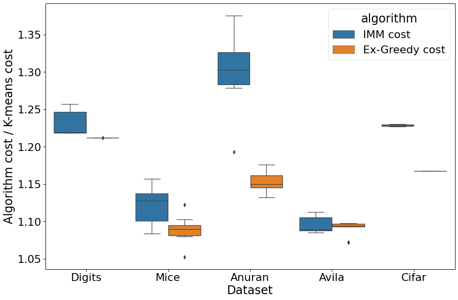
Given the success of IMM, we compared it with our method Ex-Greedy on the same datasets. The column IMM (resp. Ex-Greedy) of Table 1 shows the average ratio between the cost of the clustering obtained by IMM (resp. Ex-Greedy) and that of the initial unrestricted clustering produced by scikit-learn’s KMeans algorithm [28]. Following [15], the value of is the number of classes for the classification task associated with the dataset.
Each dataset was run for 10 iterations, with random seeds from 1 to 10, to ensure the reproducibility of results. For each iteration, we initially achieve an unrestricted solution by running the KMeans algorithm provided in the scikit-klearn package with default parameters. We then pass to the implementation of IMM from [15], available at https://github.com/navefr/ExKMC, and to our implementation of Ex-Greedy, to find two explainable clustering solutions induced by decision trees.
For 5 datasets, the results were very similar while for the others (bold in Table 1) Ex-Greedy performed better than IMM. Figure 1 presents box plots for the 5 datasets where there was a difference of at least 0.01 on the average results. It is interesting to note that the dispersion of Ex-Greedy is considerably smaller.
In terms of running time both methods spent less than 1 second, for 6 datasets. For the remaining datasets IMM was the fastest as shown in Table 2. In spite of that, we understand that Ex-Greedy is fast enough to be used in practice.
| Dataset | IMM (sec) | Ex-Greedy (sec) |
| Avila | 1.7 | 2.4 |
| Covtype | 42 | 53 |
| Newsgroups | 41 | 102 |
| CIFAR-10 | 312 | 378 |
4.2.3 Details of the experimental settings and the datasets
All our experiments were executed in a MacBook Air, 8Gb of RAM, processor 1,6 GHz Dual-Core Intel Core i5, executing macOS Catalina, version 10.15.7. Our code is availble in https://github.com/lmurtinho/ExKMC.
The datasets Iris, Wine, Breast Cancer, Digits, Covtype, Mice and Newsgroup are available in Python’s scikit-learn; Cifar-10 is available in TensorFlow; Anuran and Avila were downloaded from UCI.
For Mice, the examples with missing values were removed. For Avila, the training set and the testing set are used together. Finally, for Newsgroup, we removed headers, footers, quotes, stopwords, and words that either appear in less than or more than of the documents, following [15].
5 Maximum-Spacing Clustering
We show that the price of explainability for the maximum-spacing problem is .
5.1 Lower bound
The following simple construction shows that the price of explainability is .
Let . Moreover, for , let . The dataset for our instance is given by .
The unrestricted -clustering has spacing . On the other hand, every explainable -clustering has spacing 1. To see that, note that we cannot have all the points of in the same cluster, for otherwise we would have at most clusters. Thus, we need to separate at least 2 points from and the only way to accomplish that, via axis-aligned cuts, forces the separation of 2 points in that are at distance 1 from each other. Thus, the spacing will be 1.
Lemma 7.
The price of explainability for the maximum-spacing clustering problem is .
5.2 Upper Bound
We present an algorithm that always obtains an explainable clustering with spacing , where is the spacing of the optimal unrestricted clustering. That, together with the previous lemma, implies that the price of explainability for the maximum-spacing problem is .
Algorithm 3 receives an optimal -clustering as input and uses it as a guide to transforming an initial single cluster containing all points of into an explainable -clustering. The existence of cluster at line (*) follows from a simple pigeonhole argument. The motivation for this choice is that has two points at distance at least , which is used to show the existence of a cut with a large enough margin.
Lemma 8.
Given a set of points , Ex-SingleLink() obtains a -clustering with spacing at least , where is the spacing of an optimal unrestricted clustering.
Proof.
First, we observe that it is always possible to properly execute line (*) of Ex-SingleLink. In fact, if we pick points covering all the clusters of then, by the pigeonhole principle, two of them will lie in the same group in since has less than groups when line (*) is executed.
To establish the result it suffices to prove that there is always an axis-aligned cut that splits the selected cluster into two clusters with spacing at least .
Let and be two points in that lie in distinct clusters in and let be a graph, where is the set of points in and connects points in with distance smaller than . Moreover, let be a forest that is obtained by running Kruskal’s MST algorithm on .
Claim 2.
Points in that belong to distinct clusters of must also belong to different trees in forest .
Proof.
For the sake of contradiction we assume that the claim does not hold. In this case, there would be a path from to in and this path would have an edge joining two points that belong to different clusters in , which cannot occur since their distance is at least . ∎
The previous claim implies that since and belong to different clusters. We say that an axis-aligned cut is good with respect to a cluster if it satisfies the following properties: (i) it separates the points in into two non-empty clusters and (ii) it does not separate points that lie in the same tree of . If a good cut exists, then we can use it to split into two clusters with spacing at least since, by construction, points in different trees have distance at least . For the sake of contradiction let us assume that such a cut does not exist.
For each let be the real interval that starts in and ends in , that is, .
Moreover, for each tree in , let be the interval that starts at and ends at . Finally, for each edge in and each , let be the real interval that starts at and ends at . For a real interval , let be its length.
Since there are no good cuts, for , we have
From the triangle inequality we obtain
From the two previous inequalities we get
A simple application of Jensen inequality shows that
where is the number of edges in . By adding the above inequality for all we get
where is the distance between the two endpoints of edge .
The last inequality implies for some edge . Thus, to obtain a contradiction, it suffices to show that , since we cannot have edges in with distance
To see that , let be the number of clusters in that are singletons and let be the set of points in these clusters. Moreover, let be a set of points with each of them belonging to a different cluster in . Note that cluster is not a singleton since . Since both and are subsets of we have so that . It follows from Claim 2 that the number of trees in is at least and, as a result, its number of edges satisfies edges. ∎
We can state the main result of this section.
Theorem 5.
The price of explainability for the maximum-spacing problem is .
References
- [1] A. Adadi and M. Berrada, Peeking inside the black-box: A survey on explainable artificial intelligence (xai), IEEE Access, 6 (2018), pp. 52138–52160.
- [2] D. Aloise, A. Deshpande, P. Hansen, and P. Popat, Np-hardness of euclidean sum-of-squares clustering, Machine learning, 75 (2009), pp. 245–248.
- [3] E. Baralis, D. E. Pastor, and M. Cannone, Explainable ai for clustering algorithms.
- [4] J. Basak and R. Krishnapuram, Interpretable hierarchical clustering by constructing an unsupervised decision tree, IEEE Transactions on Knowledge and Data Engineering, 17 (2005), pp. 121–132.
- [5] D. Bertsimas and J. Dunn, Optimal classification trees, Machine Learning, 106 (2017), pp. 1039–1082.
- [6] D. Bertsimas, A. Orfanoudaki, and H. Wiberg, Interpretable clustering: an optimization approach, Machine Learning, (2020), pp. 1–50.
- [7] H. Blockeel, L. De Raedt, and J. Ramon, Top-down induction of clustering trees, arXiv preprint cs/0011032, (2000).
- [8] M. Charikar, R. Fagin, V. Guruswami, J. Kleinberg, P. Raghavan, and A. Sahai, Query strategies for priced information, Journal of Computer and System Sciences, 64 (2002), pp. 785–819.
- [9] M. Chavent, C. Guinot, Y. Lechevallier, and M. Tenenhaus, Méthodes divisives de classification et segmentation non supervisée: Recherche d’une typologie de la peau humaine saine, Revue de statistique appliquée, 47 (1999), pp. 87–99.
- [10] J. Chen, Interpretable Clustering Methods, PhD thesis, Northeastern University, 2018.
- [11] J. Chen, Y. Chang, B. Hobbs, P. Castaldi, M. Cho, E. Silverman, and J. Dy, Interpretable clustering via discriminative rectangle mixture model, in 2016 IEEE 16th International Conference on Data Mining (ICDM), IEEE, 2016, pp. 823–828.
- [12] S. Dasgupta, N. Frost, M. Moshkovitz, and C. Rashtchian, Explainable k-means clustering: Theory and practice, in XXAI: Extending Explainable AI Beyond Deep Models and Classifiers, 2020.
- [13] D. H. Fisher, Knowledge acquisition via incremental conceptual clustering, Machine learning, 2 (1987), pp. 139–172.
- [14] R. Fraiman, B. Ghattas, and M. Svarc, Interpretable clustering using unsupervised binary trees, Advances in Data Analysis and Classification, 7 (2013), pp. 125–145.
- [15] N. Frost, M. Moshkovitz, and C. Rashtchian, Exkmc: Expanding explainable -means clustering, arXiv preprint arXiv:2006.02399, (2020).
- [16] E. Horel and K. Giesecke, Computationally efficient feature significance and importance for machine learning models, 2019.
- [17] E. Horel, K. Giesecke, V. Storchan, and N. Chittar, Explainable clustering and application to wealth management compliance, 2020.
- [18] T. Kanungo, D. M. Mount, N. S. Netanyahu, C. D. Piatko, R. Silverman, and A. Y. Wu, A local search approximation algorithm for k-means clustering, Computational Geometry, 28 (2004), pp. 89–112.
- [19] J. Kauffmann, M. Esders, G. Montavon, W. Samek, and K.-R. Müller, From clustering to cluster explanations via neural networks, arXiv preprint arXiv:1906.07633, (2019).
- [20] E. S. Laber, R. L. Milidiú, and A. A. Pessoa, On binary searching with nonuniform costs, SIAM Journal on Computing, 31 (2002), pp. 1022–1047.
- [21] B. Liu, Y. Xia, and P. S. Yu, Clustering through decision tree construction, in Proceedings of the ninth international conference on Information and knowledge management, 2000, pp. 20–29.
- [22] O. Loyola-González, A. E. Gutierrez-Rodríguez, M. A. Medina-Pérez, R. Monroy, J. F. Martínez-Trinidad, J. A. Carrasco-Ochoa, and M. García-Borroto, An explainable artificial intelligence model for clustering numerical databases, IEEE Access, 8 (2020), pp. 52370–52384.
- [23] S. M. Lundberg and S.-I. Lee, A unified approach to interpreting model predictions, in Advances in neural information processing systems, 2017, pp. 4765–4774.
- [24] N. Megiddo and K. J. Supowit, On the complexity of some common geometric location problems, SIAM journal on computing, 13 (1984), pp. 182–196.
- [25] C. Molnar, Interpretable Machine Learning, Lulu.com, 2020.
- [26] M. Moshkovitz, S. Dasgupta, C. Rashtchian, and N. Frost, Explainable k-means and k-medians clustering, in Proceedings of the 37th International Conference on Machine Learning, H. D. III and A. Singh, eds., vol. 119 of Proceedings of Machine Learning Research, PMLR, 13–18 Jul 2020, pp. 7055–7065.
- [27] W. J. Murdoch, C. Singh, K. Kumbier, R. Abbasi-Asl, and B. Yu, Interpretable machine learning: definitions, methods, and applications, arXiv preprint arXiv:1901.04592, (2019).
- [28] F. Pedregosa, G. Varoquaux, A. Gramfort, V. Michel, B. Thirion, O. Grisel, M. Blondel, P. Prettenhofer, R. Weiss, V. Dubourg, J. Vanderplas, A. Passos, D. Cournapeau, M. Brucher, M. Perrot, and E. Duchesnay, Scikit-learn: Machine learning in Python, Journal of Machine Learning Research, 12 (2011), pp. 2825–2830.
- [29] D. Pelleg and A. Moore, Mixtures of rectangles: Interpretable soft clustering, in ICML, 2001, pp. 401–408.
- [30] C. Plant and C. Böhm, Inconco: Interpretable clustering of numerical and categorical objects, in Proceedings of the 17th ACM SIGKDD International Conference on Knowledge Discovery and Data Mining, KDD ’11, New York, NY, USA, 2011, Association for Computing Machinery, p. 1127–1135.
- [31] M. T. Ribeiro, S. Singh, and C. Guestrin, ” why should i trust you?” explaining the predictions of any classifier, in Proceedings of the 22nd ACM SIGKDD international conference on knowledge discovery and data mining, 2016, pp. 1135–1144.
- [32] C. Rudin, Stop explaining black box machine learning models for high stakes decisions and use interpretable models instead, Nature Machine Intelligence, 1 (2019), pp. 206–215.
- [33] S. Saisubramanian, S. Galhotra, and S. Zilberstein, Balancing the tradeoff between clustering value and interpretability, in Proceedings of the AAAI/ACM Conference on AI, Ethics, and Society, 2020, pp. 351–357.
- [34] T. Vidal and M. Schiffer, Born-again tree ensembles, in Proceedings of the 37th International Conference on Machine Learning, H. D. III and A. Singh, eds., vol. 119 of Proceedings of Machine Learning Research, Virtual, 13–18 Jul 2020, PMLR, pp. 9743–9753.
- [35] D. P. Williamson and D. B. Shmoys, The Design of Approximation Algorithms, Cambridge University Press, 2011.