Control of Stochastic Quantum Dynamics by Differentiable Programming
Abstract
Control of the stochastic dynamics of a quantum system is indispensable in fields such as quantum information processing and metrology. However, there is no general ready-made approach to the design of efficient control strategies. Here, we propose a framework for the automated design of control schemes based on differentiable programming (P). We apply this approach to the state preparation and stabilization of a qubit subjected to homodyne detection. To this end, we formulate the control task as an optimization problem where the loss function quantifies the distance from the target state, and we employ neural networks (NNs) as controllers. The system’s time evolution is governed by a stochastic differential equation (SDE). To implement efficient training, we backpropagate the gradient information from the loss function through the SDE solver using adjoint sensitivity methods. As a first example, we feed the quantum state to the controller and focus on different methods of obtaining gradients. As a second example, we directly feed the homodyne detection signal to the controller. The instantaneous value of the homodyne current contains only very limited information on the actual state of the system, masked by unavoidable photon-number fluctuations. Despite the resulting poor signal-to-noise ratio, we can train our controller to prepare and stabilize the qubit to a target state with a mean fidelity of around 85%. We also compare the solutions found by the NN to a hand-crafted control strategy.
August 11, 2026
1 Introduction
The ability to precisely prepare and manipulate quantum degrees of freedom is a prerequisite of most applications of quantum mechanics in sensing, computation, simulation and general information processing. Many relevant tasks in this area can be formulated as optimal control problems, and therefore, quantum control is a rich and very active research field, see [1, 2] for two recent textbooks that provide theoretical background and [3] for a recent review of important issues.
A typical goal of quantum control is to find a sequence of operations or parameter values (e.g. external field amplitudes) such that the quantum system under consideration is maintained in a certain target state or evolves in a desired fashion subject to additional boundary conditions (e.g. most rapid evolution for a prescribed maximal strength of the control fields). In the case of feedback control the control sequence is determined based on a signal coming from the system [3, 4]. The control task and its boundary conditions are typically specified by a loss function. To cast the optimal control problem into an optimization task, one then introduces a parametric ansatz for feedback schemes, also known as controllers, and explores the parameter space to minimize the loss function.
Reinforcement learning (RL) [5, 6] has been proposed as a suitable framework to develop control strategies. In this framework, the controller (or agent), optimizes its strategy (the policy) based on the loss function (the rewards) obtained from repetitive interactions with the system to be controlled. In the context of quantum physics, RL has proven useful, e.g. for reducing the error rate in quantum gate synthesis [7], for autonomous preparation of Floquet-engineered states [8], and for optimal manipulation of many-qubit systems [9]. RL is a black-box setting, i.e. the agent has no prior knowledge on the structure of the system it interacts with, and has to develop its policy (explore the space of control parameters) only relying on its past interactions with the system. This makes RL very versatile but requires a large number of training episodes to find a good strategy.
Optimal control design is rarely done on an (unknown) system in situ. Instead one trains the controller on a physical model of the real system. This means that rather than learning how to interact with an unknown environment, one actually starts with a lot of prior scientific knowledge about the system, namely its precise dynamical model. In the simplest cases, one can even solve the optimal control problem for this model analytically. Generally, using prior information leads to more data-efficient training [10, 11]. In the context of the present paper, we use the physical model of the system to efficiently compute the loss function’s gradients with respect to the parameters of the controller ansatz. Naturally, having access to the gradients of the loss function can streamline the optimal control design tremendously.
In the case of quantum control the model consist of a quantum state space and a parametric equation of motion. The dynamics of the system can be solved for fixed values of the parameters of the model and of the controller. Usually, this is done numerically. Then, the most naive way to obtain the loss function’s gradients is to solve the dynamics for a set of parameter values in the neighborhood of each point and use finite difference quotients. Yet, this method is unfeasible if the number of parameters is large, it suffers from floating-point errors, and it may be numerically unstable. To circumvent these issues, automatic differentiation (AD) has been proposed as another approach to calculate gradients numerically [12, 13], a paradigm also known as differentiable programming (P) [14, 15]. By backpropagating the loss function’s sensitivity through the numerical simulation, one can compute the gradients with similar time complexity as solving the system’s dynamics [16]. Recently, these techniques have been merged with deep neural networks (NNs) as ansatz for the controllers [10, 17, 18]. This is possible because the training of deep NNs is based on stochastic gradient descent through a large parameter space and becomes efficient when used in conjunction with P-compatible solvers for the system’s dynamics.
In this work, we develop such a physics-informed reinforcement learning framework based on P and NNs to control the stochastic dynamics of a quantum system under continuous monitoring [2, 19]. Continuous measurements, such as photon counting and homodyne detection, allow one to gain information on the random evolution of a dissipative quantum system [2]. This information can be used to estimate the state of the quantum system [20, 21, 22], to implement feedback protocols [23, 24, 25, 26, 27], to generate nonclassical states [28, 29, 30, 31], and to implement teleportation protocols [32, 33]. Continuous homodyne detection can be realized experimentally in the microwave [34, 35] and optical regime [20, 36]. The time evolution of a monitored quantum system is described by quantum trajectories, which are solutions of differential equations driven by a Lévy process.
To illustrate our framework, we focus on a qubit subjected to continuous homodyne detection [34, 37] described by a stochastic Schrödinger equation. We engineer a controller which provides a control scheme to fulfil a given state preparation task based on the measured homodyne current. This situation extends an earlier study [10], where it has been demonstrated that P can be efficiently used for quantum control in the context of (unitary) closed-system dynamics, i.e. when the dynamics follows an ordinary differential equation. The stochastic nature of the problem analyzed here renders the control task more challenging because the controller must adapt to the random evolution of the quantum state in each trajectory. Moreover, the instantaneous value of the homodyne current does not determine the actual state of the qubit. It is correlated only to the projection of the state onto the -axis and this signal is hidden in the noise which dominates the measured homodyne current [38, 39]. Thus, the information about the state of the qubit at a given time must be filtered out from the time series of measurement results.
This paper is organized as follows: In Section 2, we describe the proposed setup of a qubit in a leaky cavity subjected to homodyne detection and derive the stochastic Schrödinger equation that describes its dynamics. We then discuss two ways to use the record of the homodyne detection signal in a feedback scheme to engineer a drive that can be applied to the qubit to perform a desired control task, e.g. state preparation or stabilization. We also introduce the concept of adjoint sensitivity methods that we use to efficiently compute gradients with respect to solutions of SDEs. Section 3 describes the first feedback scheme in detail: Here, we assume that the controller has direct access to the quantum state, e.g. through an appropriate filtering procedure applied to the measurement records. We compare three strategies, viz. a hand-crafted control scheme, one in which a neural network continuously updates the control drive based on the knowledge of the state, and a numerically less demanding one with a piecewise-constant control drive. Section 4 presents the second feedback scheme where directly the measurement record of the homodyne current is fed to the NN representing the controller. In this setup, the NN must first learn how to filter the data to obtain information on the state of the system. Only after that it can propose an efficient control strategy. We conclude in Section 5 and discuss potential future applications.
2 Theoretical background
2.1 A qubit under homodyne detection
We consider a driven two-level system with states and . In a rotating frame, its Hamiltonian reads
| (1) |
where are Pauli matrices, is the Rabi frequency of the drive laser, and is the detuning between the qubit and the laser. The qubit can spontaneously decay into a photon field via the interaction Hamiltonian
| (2) |
where is the decay rate. The field operators and satisfy the commutation relation . We assume that the field is initially in the vacuum state, . Physical examples of such a system are a two-level atom inside a leaky single-mode cavity that can be adiabatically eliminated, or an artificial atom, e.g. a superconducting qubit, coupled to a waveguide. The radiation emitted from the two-level system is monitored with a continuous homodyne measurement, as depicted in Fig. 1(a).
We show in A (see also [2, 19]) that the evolution of the qubit is governed by a stochastic Schrödinger equation
| (3) |
where denotes an unnormalized qubit state. The instantaneous value of the measured homodyne current is a random variable satisfying
| (4) |
Here, is the expectation value of at time , and is a stochastic white-noise term satisfying , which stems from the shot noise of the local oscillator. Heuristically, can be considered as the derivative of a stochastic Wiener increment, , such that the contribution of the noise to the current integrated over a short time interval is described by a Wiener process,
| (5) |
The ensemble averages of the stochastic Wiener increment satisfy and . Several remarks are in order to better understand the dynamics of the system.
First, Eq. (5) implies that the value of the current over a short interval contains only very little information about the state of the qubit. This can be seen from the (heuristically stated) vanishing signal-to-noise ratio
| (6) |
If was a constant signal, one could simply integrate the current over a time interval longer than to increase the signal-to-noise ratio. However, this is not possible because relaxation will change the state of the two-level system on the time scale . Thus, the low signal-to-noise ratio is an intrinsic feature of this homodyne detection scheme. This is illustrated in Figs. 1(c) and (d), where we show a simulation of the homodyne current together with the respective value for a single quantum trajectory.
Second, Eq. (3) shows that the infinitesimal time evolution and thus the quantum trajectory is fully determined by the record of the measured homodyne current and the values of the applied drive , which are vectors containing the respective values of and from the start time until the time . In A.4, we derive a closed-form expression of the operator , which gives the mapping
| (7) |
between the states of the qubit at times and . The operator can be interpreted as a filter determining the state of the qubit at time from the values of the measured homodyne current and the applied drive.
Finally, Eq. (3) does not preserve the norm of the state , as indicated by the tilde. This is no problem if one integrates Eq. (3) numerically, since one can renormalize the state after each time step. For analytical calculations, it is useful to add some correction terms (see A.5 or [2, 19]) such that the norm of the state is preserved up to second order in ,
| (8) |
Here, the nonlinear drift and diffusion terms are
| (9) | ||||
| (10) |
Note that Eq. (8) is a stochastic Schrödinger equation in the Itô form with multiplicative scalar noise.
2.2 Feedback control overview
In our control protocol, the results of the homodyne detection measurement determine the drive to be applied to the qubit. We will consider two different schemes which are sketched in Fig. 1(b).
In the first scheme, discussed in Section 3, we filter the homodyne signal to extract the system’s exact state at time . Subsequently, the controller receives this state as an input and determines the drive to be applied next. Equations (7) and (55) give an explicit filtering procedure to determine the state of the qubit at time from the records of homodyne measurements and the drive , which are known in the experiment. Since we train the agent on simulated trajectories, we know the system’s state at each time step. Therefore, we can skip the filter in Fig. 1(b) and directly feed back the solution of the SDE solver at each time step to our controller. In other words we assume a perfect filtering at any time. Thus, this situation corresponds to the feedback used in Ref. [10] but the deterministic evolution is replaced by an SDE. We will use this control scheme in Section 3 to test different backpropagation methods and to compare different control strategies.
In the second scheme, discussed in Section 4, the controller obtains at time the homodyne current record measured over some time interval . Now, the NN forming the controller must simultaneously learn how to filter the signal from the noise and to predict the next action . Such an implementation of the control protocol based only on is a challenging task because the signal of the system quadrature is hidden in the noise as discussed in Section 2.1.
2.3 Workflow

The learning scheme to control the stochastic dynamics of the continuously monitored qubit based on P consists of three building blocks as sketched in Fig. 2: a parametrized controller , which will be formed by a NN, a model of the dynamics, expressed as an SDE, and a loss function.
At the beginning of each run, we initialize the system in an arbitrary state on the Bloch sphere,
| (11) |
where and are the excited and ground states of the qubit in the -basis, respectively. To ensure that the controller will perform optimally for any initial state, we sample the angles and uniformly from their intervals and , respectively.
Depending on the chosen control scheme, cf. Fig. 1(b), the controller receives as an input either the quantum state (Section 3) or the last homodyne detection record in form of a vector gathered over some time interval (Section 4). Moreover, in Section 4 the controller also receives a vector of the last control actions applied prior to the time .
The controller then maps this input to the next value of the drive, . Given and , we use the Runge-Kutta Milstein solver from the StochasticDiffEq.jl package [40, 41, 42] to calculate the next state according to the SDE (8). This loop between control agent and SDE solver is iterated for all time steps. We store the quantum states and the drive values at uniformly spaced time steps to be able to evaluate the loss function. Hereafter, the set is called checkpoints.
We minimize a loss function of the form [10, 12, 13, 43]
| (12) |
where the terms encode case-specific objectives of the optimization process, see, e.g. Ref. [12]. Their relative importance can be controlled by the weights . We choose the weights empirically but, if necessary, they could also be tuned by means of hyperparameter optimization techniques [10]. To enforce a large fidelity with respect to the target state over the whole control interval, we include into the loss function the average infidelity of the checkpoints with respect to the target state ,
| (13) |
This form of the loss function also leads to a time-optimal performance of the controller. To focus on specific time intervals, like the last few steps for example, the sum in Eq. (13) can be straightforwardly adjusted. We will consider the target state in the following. In addition to , we include the term
| (14) |
in the loss function to favor smaller amplitudes of the drive . In Section 4, we will find that this term is important to suppress the collapse of the NN towards a strategy where constant maximal pulses are applied during the training.
At this stage, we have calculated a quantum trajectory and evaluated its value of the loss function. In the next step, we must update the control strategy to decrease the value of the loss function. The derivative of the loss function with respect to the parameters of the neural network provides a meaningful update rule towards a better control strategy. Thus, we need to calculate the gradient . This can be computed efficiently using sensitivity methods for SDEs discussed next.
2.4 Adjoint sensitivity methods
The loss function , defined in Eq. (12), is a scalar function which explicitly depends on the checkpoints and implicitly on the parameters of the controller. In contrast to score-function estimators [44, 45, 46], such as the REINFORCE algorithm [47], we will incorporate the physical model into the gradient computation as sketched in Fig. 2.
Automatic differentiation (AD) is a powerful tool to evaluate gradients of numeric functions at machine precision [48]. A key concept to AD is the computational graph [49], also known as Wengert trace, which is a directed acyclic graph that represents the sequence of elementary operations that a computer program applies to its input values to calculate its output values. The nodes of the computational graph are the elementary computational steps of the program called primitives. The outcome of each primitive operation, called an intermediate variable, is evaluated in the forward pass through the graph.
In forward-mode AD, one associates with each intermediate variable the value of the derivative
| (15) |
with respect to a parameter of interest. The derivatives are calculated together with the associated intermediate values in the forward pass, i.e. the gradient is pushed forward through the graph. This procedure must be repeated for each parameter , therefore, forward-mode AD scales poorly in computation time with increasing number of parameters .
In contrast, reverse-mode AD traverses the computation graph backwards from the loss function to the parameters by defining an adjoint process:
| (16) |
which is the sensitivity of the loss function with respect to changes in the intermediate variable . Reverse-mode AD is very efficient in terms of the number of input parameters because one needs just a single backward pass after the forward pass to obtain the gradient with respect to all parameters . Thus, we always implement the AD of the NN in reverse mode. However, reverse-mode AD might be very memory expensive because all intermediate variables from the forward pass need to be stored for the backward pass. Therefore, reverse-mode AD scales poorly in memory if the number of steps and parameters of the SDE solver increases. Whether forward-mode or reverse-mode AD is more efficient to calculate gradients of the loss function depends on the specific details of the control loop shown in Fig. 2.
In fact, it is possible to combine different AD methods on different parts of the computational graph as we illustrate now. In Secs. 3.3 and 4, we will use Algorithm 1, where the drive is piecewise constant, i.e. a constant value of is applied over successive time steps between two checkpoints. In this case, the memory consumption of the reverse-mode AD of the NN is moderate since the number of parameters grows only with the number of checkpoints rather than with the number of time steps. In contrast, in the SDE solver the evaluation of the time evolution between two checkpoints and only depends on the single parameter , which makes forward-mode AD very efficient [50]. Therefore, we nest both methods and use an inner forward-mode AD through the SDE solver and an outer reverse-mode AD for the remaining parts, i.e. the NN and the computation of the loss function.
Restricting oneself to a piecewise-constant control drive, however, prevents the controller from reacting instantaneously to changes of the state. To implement a fast control loop, the controller has to be placed in the drift term of the SDE (8). Thus, the parameters entering the solver will be the NN parameters , see Algorithm 2. The continuous adjoint sensitivity method [51, 52, 53] circumvents the resulting memory issues by introducing a new primitive for the whole SDE in the backward pass of the code. This new primitive is determined by the solution of another SDE problem, the adjoint SDE. Formally, defining the adjoint process as
| (17) |
the adjoint SDE problem in the Itô sense satisfies the differential equation
| (18) |
with the initial condition
| (19) |
where the standard conversion factor in Eq. (18) accounts for the required transformation from the Itô to the Stratonovich sense and vice versa [54]. The gradients of the loss function with respect to are then determined by the integration of
| (20) |
with the initial condition . This continuous adjoint sensitivity method will be used in Section 3.2. Further details regarding the adjoint method and our Julia implementation [55, 56] within the SciML ecosystem [11, 16, 40] are discussed in C.2.
3 SDE control based on full knowledge of the state
We first investigate the scenario in which the controller maps the quantum state to a new control parameter, . From a learning perspective, this is a major simplification because the NN does not need to learn how to filter the homodyne current to determine the state . From a practical perspective of controller design, this approach assumes that there is already a filter module, which allows one to predict the state of the system from the measurement record and past control actions. We discuss in Section 2.1 and A.4 the implementation of such a filter in our case of a qubit subjected to homodyne detection. Note that if the initial state of the qubit is unknown, only a mixed state can be obtained if the detection record is too short. Nevertheless, it is always possible to obtain a pure state estimate and recover our scenario, e.g. by projecting onto the surface of the Bloch sphere. Alternatively, one can straightforwardly generalize our approach to the case of a stochastic quantum master equation describing the evolution of the system’s density matrix in the presence of homodyne detection, cf. A.5.
For all numerical experiments we fix the parameters of the physical model as and . We discuss the variation of these parameters and their impact on the reached fidelity in D.
3.1 Hand-crafted strategy

The control operator in Eq. (1) induces a rotation about the -axis. Therefore, a simple but very intuitive strategy to move the state upwards in each time step is to compute the expectation value and to choose the direction of rotation depending on its sign. Specifically, if (or ), the controller should rotate (counter-) clockwise about the -axis, as summarized in Algorithm 3.
Figure 3(a,b) shows the fidelity and the associated drive for this control scheme. Though conceptually straightforward, this hand-crafted control function is very efficient. The mean fidelity over the whole control interval is . We visualize the control strategy in Fig. 3(c), where we show the applied drive as a function of the state on the Bloch sphere. The Bloch sphere [with spherical coordinates , see also Eq. (11)] is mapped onto the tangential plane at , described by polar coordinates , using a stereographic projection
| (21) |
Apparently, the stereographic projection maps the south pole to and the north pole to . Throughout this paper we truncate the value of to an interval , so we plot the applied drive values on the states of the southern hemisphere, cf. Fig. 3(c,d).
3.2 Continuously updated control drive

Now we apply a NN as the controller. We use a controller which changes in every time step of the solver based on the current state . This implements a high-frequency feedback loop but renders discrete AD methods very inefficient since all parameters of the NN contribute to the feedback loop. Consequently, we use the continuous adjoint sensitivity methods described in Section 2.4 to calculate gradients of the loss function.
Figure 4(a) shows the smooth evolution of the loss function throughout the training of the (fully-connected) neural network, which converges to a configuration able to reach quickly fidelities with mean value of about with modest standard deviation, see Fig. 4(b). The mean fidelity over the whole control interval is . Figure 4(c) illustrates the applied drive during this time evolution. The inset of Fig. 4(a) visualizes the control strategy on the Bloch sphere. The same is depicted in Fig. 3(d) using the stereographic projection, see Eq. (21). The controlled evolution of the initial state , corresponding to the black lines in Fig. 4(b,c), is marked by the yellow points. These points show how the controller first transfers the state from the south pole to the north pole region and then stabilizes it in vicinity of the target state .
3.3 Piecewise-constant control drive
Now we reduce the control frequency and assume that the controller changes the action only every time steps. This case is crucial in many physical situations, where the control loop is not fast enough to follow high-frequency changes in the physical system. In practice this means that we evolve the state for substeps between the checkpoints with fixed value of . The resulting piecewise-constant control scheme allows us to use the discrete forward-mode adjoint sensitivity method through the SDE solver combined with an outer reverse-mode AD through the rest of the control loop, as described in Section 2.4. Although we restricted the rate at which can change, we find that the NN converges to a similar learning behavior with similarly large fidelities as in Section 3.2, see Fig. 4(e). The mean fidelity over the whole control interval is .
3.4 Comparison of the control strategies
Based on the results from a set of 256 trajectories, all three control strategies perform nearly equally well in terms of their average fidelities F 0.9. The piecewise-constant controller slightly outperforms the other two approaches by having the smallest relative dispersion of the mean fidelity , which we attribute to the larger number of training epochs and the larger NN, see Table 1.
The hand-crafted strategy achieves a large average fidelity, but generates sudden jumps in the drive , as shown in Fig. 3(b). Such a drive is experimentally hardly feasible. We find that NNs with moderate depths provide a smooth mapping between the input states and the drive, see Figs. 3(c) vs. 3(d), while keeping high fidelity in the control interval. The signals generated by these protocols are experimentally more accessible, see Figs. 4(d) and (f). When necessary, specific terms can be added to in Eq. (12) to strengthen various requirements on the controller’s performance (e.g. the smoothness of the drive or bounds on the power input) as discussed in Section 2.2. This is not the case for the hand-crafted strategies where an efficient implementation of these constraints might be impossible. Furthermore, in some cases, e.g. the mountain car problem, it is not straightforward to come up with any hand-crafted strategy to start with. In contrast, the RL and P approach is easily adjustable to different physical systems.
There are two principal reasons why the fidelity only reaches 0.9 in our setup. First, is a time-average and the controller needs some time to align the qubit to a target state (starting from an arbitrary state). Second, the controlled qubit rotates about an axis in the --plane whose direction depends on the ratio . Hence, even in the case when the qubit rotates solely about the -axis, the drive can only bring the qubit all the way up to the north pole of the Bloch sphere if the current state lies on a great circle perpendicular to this axis. Therefore, the ratio and the maximum value of set a limit on how close the qubit can come to the target state on average. In D, we study scenarios with lower and observe that the average fidelity can increase and approach unity. We can thus conclude that is not a limit of our design but rather originates from the restricted capability of control operations considered here.
4 SDE control based on homodyne current
In this section, we will construct a controller which directly obtains the (noisy) measurement record of the homodyne current and determines the optimal control field in each time interval . We consider a controller formed by a slightly augmented NN architecture with fully connected layers (see Fig. 6). The acquisition of input data for the NN consists of the following steps:
- 1.
The controller generates a piecewise-constant drive between two checkpoints at times and , as described in Section 3.3. In the time window , we integrate the SDE (8) using substeps of length as sketched in Fig. 5(a). We label these substeps with . The input for the NN to predict the next is a vector where is the length of the time interval over which we gather the data. Experimentally, can be interpreted as the detection time window of the photodetectors. According to Eqs. (4) and (5), the homodyne measurement in the th substep is
(22) The first term corresponds to the quadrature signal measured over the detection window , which we assume to be approximately constant on time scales of the order of . The second term is the Wiener increment during the th substep. Note that the quantity is dimensionless and solely represents the number of measured detected photons, as discussed in A.
- 2.
In addition, we provide the NN with the information on the last control parameters . This equips the NN with a “memory” of its own actions, such that it can take into account how a sequence of the last control drive amplitudes affected the performance. We empirically choose such that the length of the input vector corresponds to of the length of .
Given these inputs, the task for the controller is to provide an optimal mapping . Figure 5(b) shows the evolution of the loss function during the learning phase as a function of the training epochs. Note that there are two distinct plateaus. First, after a couple of hundred epochs, the NN develops a general strategy consisting of the application of a periodic drive to prevent the qubit from decaying to the ground state. Figures 5(c,d) show examples of the performance of the NN at epoch to illustrate this phase of the training. This strategy is state-independent, yet it manages to keep the mean fidelity of the simulated trajectories around over the whole control interval. Around epoch , after some transition phase where oscillates substantially, the NN starts to provide state-sensitive control fields. The final performance of the controller in Fig. 5(e,f) reaches the mean fidelity over the whole control interval. During the last 50 time steps in the control interval, which we specifically focus on during the training using the adjusted loss function term of the type (13) for these steps, the average fidelity is .
At this stage, we infer that the NN has learnt how to extract the signal from the noisy data before it attains a similar learning strategy as seen in Section 3. In contrast to the filter mentioned in Section 2.1 and A.4, this universal approach based on P will also work if some parameters of the model were a priori unknown. For example, if the detuning was unknown, one could train the controller on an ensemble of randomly chosen parameters , such that it learns how to deal with the general situation of arbitrary detuning. In this case a straightforward filtering of the signals to obtain the state is unfeasible, as this would require to solve the filter for all possible values of model parameters, cf. Eq. (55). Other options for signal filtering would be (recursive) backward filtering methods [57, 58] or recurrent neural networks because their structure allows them to capture temporal correlations in the data [39]. Note that such filter methods are compatible with the two-step control approach described in Section 3.
5 Discussion
In this work we proposed a framework based on differentiable programming (P) to automatically design feedback control protocols for stochastic quantum dynamics. As a test bed, we used a qubit subjected to homodyne detection, whose dynamics is given by a stochastic Schrödinger equation. Note, however, that our method can straightforwardly be applied to different physical systems and that it can be generalized to the case of stochastic quantum master equations.
In Section 3, we demonstrated that a controller, formed by a NN, can be trained to prepare and stabilize a target state starting from an arbitrary initial state of the system when the NN obtains the full knowledge of the instantaneous state at any time. The method generates a smooth drive while maintaining a high fidelity with the target state over the whole control interval. Additional constraints on the performance of the controller can be implemented by adding further terms to the loss function. This makes the P approach more versatile than tailoring control functions manually, which requires a unique approach for every new system and can even be infeasible for large quantum systems.
The key feature of our P framework is to include an explicit model of the system’s dynamics into the computation of the gradients of the loss function with respect to the parameters of the NN, i.e. the controller. Specifically, in Section 3.2, we employed the recently developed continuous adjoint sensitivity method for the gradient estimation through an SDE solver, which is memory efficient and, thus, allows us to study a high-frequency controller. F.S. implemented these new continuous adjoint sensitivity methods in the DiffEqSensitivity.jl package within the open-source SciML ecosystem [55].
In Section 4, we showed that the feedback control scheme can be based directly on providing the NN with a record of homodyne current measurements without the need to filter the information on the actual state beforehand. Therefore, the NN must first learn how to filter the input data (with poor signal-to-noise ratio) before it can predict optimal state-dependent values of the control drive. Ultimately, the trained NN was able to reach fidelities above in a target time interval for random initial states.
In future studies, the optimization of the loss function based on stochastic trajectories using adjoint sensitivity methods could be compared to alternative approaches. First, the solution to the stochastic optimal control problem in the specific case of Markovian feedback (as in Section 3) is a Hamilton-Jacobi-Bellman equation [11, 54]. The solution of this partial differential equation, with same dimension as the original SDE, may directly give the optimal drive [59]. However, solving this partial differential equation with a mesh-based technique is computationally demanding and mesh-free methods, e.g. based on NNs also require a (potentially costly) training procedure [60]. Second, the expected values of the loss functions could be optimized by leveraging the Koopman expectation for direct computation of expected values from stochastic and uncertain models [61]. Additionally, one could approach this control problem by using an SDE moment expansion to generate ordinary differential equations for the moments and apply a closure relationship [62]. Additional research is required to ascertain the efficiency of these approaches in comparison to our method.
The results reported in this paper imply that P is a powerful tool for the automated design of quantum control protocols. Further experimental needs, e.g. finite time lag between the measurement and the applied drive, finite-temperature effects, or imperfect homodyne detection, can be incorporated straightforwardly into this method. Thus, our work introduces a new perspective on how prior physical knowledge can be encoded into machine learning tools to construct a universal control framework. Besides the control application demonstrated here, the P paradigm can be also adopted to solve other inverse problems such as estimating model parameters from experimental data [63, 64, 65]. An interesting perspective for future work is to extend our framework to control-assisted quantum sensing and metrology.
Acknowledgment
We would like to thank Niels Lörch, Eliska Greplova, Moritz Schauer, and Chris Rackauckas for helpful discussions. We acknowledge financial support from the Swiss National Science Foundation (SNSF) and the NCCR Quantum Science and Technology. Parts of the computations were performed at sciCORE (scicore.unibas.ch) scientific computing core facility at University of Basel.
Data availability statement
The codes that support the findings of this study are openly available [66].
Appendix A Continuous homodyne detection
A.1 Quantum trajectories: monitoring the spontaneous emission of a qubit
Consider a two-level atom interacting with a free photon. In the case of discrete photon modes, the interaction is given by the usual Hamiltonian with and being the bosonic creation and annihilation operators, respectively, fulfilling the commutation relation , and being a coupling constant with dimension of energy. In contrast to the notation used in the main text, in this appendix, we will mark operators by a hat to distinguish them from scalars. This Hamiltonian results from the dipole interaction written in the form and application of the rotating wave approximation. However, when addressing a decay to the continuum, the photons are represented by quantum field operators with commutation relation , thus having units of square root of energy (or, equivalently, inverse square root of time). The interaction Hamiltonian takes the form
| (23) |
where is the decay rate, again, with dimension of energy like .
The field propagator in the interaction picture can be formally written as , where is the time-ordering operator. Expanding for short times , we find
| (24) |
Here, the second-order terms give an important contribution. Higher-order terms only contribute as and can be safely neglected, and we also assume that is short on the timescale of internal qubit dynamics. Assuming the free field is originally in the vacuum state we can write
| (25) |
is a properly normalized state of the field, and denotes the excited qubit state.
The simplest way to monitor the qubit state is then to continuously measure the intensity of the outgoing field. This defines a Poissonian process, as the probability to detect a photon in a time interval reads
| (26) |
and the probability of no detection is respectively. Thus, we obtain the standard unraveling for the spontaneous decay process
| (27) |
A.2 Weak homodyning
An alternative to photon-counting detection is to mix the outgoing light with coherent light from a local-oscillator laser on a beamsplitter, and to measure the intensities at both output ports of the beamsplitter. As a warm-up we first consider the situation where the intensity of the local-oscillator field is comparable to the emitted light. It is given by the expansion of a coherent state using only vacuum and single-photon states
| (28) |
where the single-photon state of the -mode is defined identically to the mode . Mixing the two states on a 50:50 beamsplitter gives
| (29) |
Introducing the photocurrent variable , which measures the intensity difference of the two outputs, we see that there are three possibilities, . The respective probabilities of the three outcomes are given by the norms of the three different terms in Eq. (29),
| (30) |
The three possible states of the system after the measurement are proportional to
| (31) |
By setting (i.e. no mixing with a local-oscillator field), we recover the previous case where the qubit simply has a chance to decay
| (32) |
and . The only difference is that the emitted photon is randomly split between the two detectors, with no information about the state of the qubit contained in the sign of .
A.3 Strong homodyning
Finally, we consider the situation treated in the main text. The standard homodyne measurement requires mixing the signal with a strong coherent local-oscillator field
| (33) |
Recall that here the Fock states are defined with the creation operator , describing the field impinging on the lower port of the beamsplitter during the interval , see Fig. 1(a). For the modes and to match, the local-oscillator laser has to be in resonance with the drive laser because, in the lab frame, the field picks up the phase of rotating at the frequency of the drive laser.
When the modes match, the 50:50 beamsplitter transformation takes the form
| (34) |
In particular, this implies , i.e. a coherent state of the mode is split into two coherent states of half the intensity when mixed with the vacuum state of the mode on a 50:50 beamsplitter. Using the last two expressions, we can write down the overall state of the qubit, the spontaneously emitted radiation and the homodyne laser field after the beamsplitter. To do so, let us compute
| (35) |
which is the operator mapping the state of the qubit at time to the state of the qubit and the two detected modes at time . We can further simplify this expression by noting that
| (36) |
where is the photon number operator. Labeling the photon number operator for the mode as , we can then rewrite Eq. (35) in a very intuitive form
| (37) |
Again, directly gives us the state of the qubit and the detected modes, while
| (38) |
gives the conditional state of the qubit together with the probability to detect and photons respectively. In the measurement process, superpositions of states with different photon numbers collapse such that the state after the post-measurement is a classical statistical mixture of the possible outcomes,
| (39) |
One easily sees from Eq. (37) that , i.e. only the difference of the photon counts reveals information on the state of the qubit, while the sum only describes the shot noise of the local oscillator. It is therefore sufficient to keep the difference and discard the sum, which defines the state
| (40) |
In a slight abuse of notation we can formally introduce the joint quantum state of the qubit and the count difference as with
| (41) |
, which gives rise to the same post-measurement state. Here,
| (42) |
where is the modified Bessel function of the first kind.
Next, we use that the distribution of on the right-hand side of Eq. (42) is well approximated by the normal distribution in the limit . Therefore, we can replace the state of an integer-valued in Eq. (41) with
| (43) |
of a continuously valued and normally distributed , and we also introduce a continuously valued operator . In the regime of interest the actual value of does not play a role. To get rid of it, recall that is the intensity of the local-oscillator laser in the time window , so it is more convenient to work with the laser power , which is independent of the choice of the time window . Then, we can rescale the photon count difference to
| (44) |
to get rid of the laser intensity. Equation (41) now reads
| (45) |
where the initial state of the rescaled can be obtained form Eq. (43) and satisfies
| (46) |
This also allows us to define the homodyne current of the main text , as the photon count difference per time. At this point note that Eq. (45) already implies Eq. (3). Let us now show how the measured value of is distributed. The marginal distribution of after the measurement reads
| (47) |
From one easily deduces the expected value and the variance of
| (48) |
Clearly, it has the form of a Wiener process with drift
| (49) |
where is the increment of a Wiener process for an interval (a normally distributed random variable with zero mean and variance ). The last step is to include the Hamiltonian of the qubit and set such that in order to get
| (50) |
A.4 Formal solution of the stochastic dynamics as a filter
The expression of the infinitesimal time evolution we just derived can be composed for all time intervals to define the evolution over a long period
| (51) |
where each time step introduces a new quantum system for the photon detection difference measured during the corresponding infinitesimal interval. The joint state of the qubit and all values of the observed homodyne current for at the final time reads
| (52) |
Hence, for any fixed values of the measured current we can find the (unnormalized) state of the qubit conditioned on these outcomes
| (53) |
and is a scalar independent of the input state . Thus, the state of the qubit at time conditioned on the homodyne detection record reads
| (54) |
and for mixed initial states . The expression of the operator
| (55) |
can be thought of as a filter relating the record of the drive fields and the values of the measured homodyne current to the map between the states of the qubit at times and , represented here by a two-by-two complex matrix. In a real experiment can be computed by, e.g. discretizing the integral.
Notably, even if the initial state of the qubit is unknown, e.g. , after a certain characteristic time the state
| (56) |
becomes pure. This is because the stochastic dynamics essentially decouples the state of the system at time from its state in a far-away past. On the other hand the measured homodyne current reveals information about the unknown initial state and we have just shown how to filter this information, as
| (57) |
for any two initial states and .
A.5 Derivation of the norm-preserving stochastic Schrödinger equation
We start with the stochastic Schrödinger equation (3) which does not preserve the norm of the state . Using
| (58) |
we can derive the corresponding stochastic quantum master equation
| (59) |
which does not preserve the norm of the density matrix. Note that the last term in Eq. (58) contains a contribution of order since . The last term in Eq. (59) shows that the state depends on the homodyne signal , but it does not preserve the norm of during the time evolution. This can be compensated by adding a correction term
| (60) |
which cancels the last term in Eq. (59) without introducing any new norm-nonconserving terms. On the level of the stochastic Schrödinger equation, this term can be generated by adding a contribution
| (61) |
which gives rise to Eq. (8) of the main text.
Appendix B Neural network architectures and hyperparameters
The hyperparameters used in the control tasks are summarized in Tab. 1. The architecture of the NN used in Section 4 is shown in Fig. 6. In all NNs, we use ReLUs as activation functions for hidden layers and the softsign activation function for the last layer. Modifications of this simple architecture, e.g. through the application of recurrent neural networks to capture temporal correlations in the homodyne current for the SDE control in Section 4, might be essential for the control of complex many-body quantum systems.
In this work, we used NNs as universal function approximators. While this approach is very general, other choices of a controller, e.g. Chebychev polynomials or Fourier basis expansions, could boost the performance for low-dimensional inputs as in the case of a qubit, because they can be optimized to the problem at hand. The use of the sparse identification for dynamical system method [67, 68, 69] or symbolic regression tools [70] could further allow one to replace the trained NNs by a symbolic description based on a pre-defined library of operators.
| (SDE) | (SDE) | (ODE) | ||||
| Section 3.2 | Section 3.3 | Section 4 | C.1 | |||
| solver | ||||||
| scheme | EulerHeun | RKMil | RKMil | Tsit5 | ||
| 200 | 20 | 80 | ||||
| adaptive | ||||||
| loss function | ||||||
| 1 | 0.8 | 1.2 | 1 | |||
| 0 | 0 | |||||
| 0 | 0 | |||||
| Adam optimizer | ||||||
| learning rate | 0.0015 | 0.0001 | 0.0001 | 0.0015 | ||
| batchsize | 64 | 64 | 64 | 256 | ||
| epochs | 1000 | 3000 | 14000 | 400 | ||
| NN | ||||||
| LLS 1 | (4, 256) | (4, 256) | (, 256) | (4, 256) | ||
| LLS 2 | (256, 64) | (256, 128) | (256, 256) | (256, 64) | ||
| LLS 3 | (64, 1) | (128,64) | (256, 128) | (64, 1) | ||
| LLS 4 | (64, 1) | |||||
| LLA 1 | (/10, 128) | |||||
| LLA 2 | (128, 128) | |||||
| LLC 1 | (256, 64) | |||||
| LLC 2 | (64, 32) | |||||
| LLC 3 | (32, 1) | |||||
Appendix C Continuous adjoint sensitivity method for ODEs and SDEs
In this appendix, we discuss the continuous adjoint sensitivity method for ordinary differential equations (ODEs) and its generalization to SDEs used in the main text. In C.1, the continuous adjoint sensitivity method for ODEs is used to compare the stochastic control scenario discussed in Section 3.2 with the associated unitary control scenario in the case of a closed system. In C.2, we provide an intuitive understanding for the stochastic adjoint process and discuss technical details regarding the continuous adjoint sensitivity method for SDEs and its implementation [55]. In all implementations, we use an isomorphism to map the complex amplitudes of the quantum state to real numbers, as required by the AD backend [71].
C.1 Quantum control of a qubit in a closed system
In this section, we aim at controlling the closed-system dynamics of a qubit given by the Schrödinger equation
| (62) |
with Hamiltonian
| (63) |
where is the qubit transition frequency [10]. As in Section 3.2, we choose a NN with parameters as the controller ansatz and we allow the NN to change the control drive in every time step based on the state . The initial states are uniformly distributed on the Bloch sphere, see Eq. (11). We compute the forward pass, Eq. (62), with the adaptive Tsitouras 5/4 embedded Runge-Kutta (Tsit5) scheme as implemented in the DifferentialEquations.jl package [40]. Given this solution, we use the loss function (12) with weights . As discussed in Section 2.3, it depends on the checkpoints at times , .
As discussed in Section 2.4, the continuous adjoint sensitivity method circumvents the memory issues of discrete reverse-mode AD and scales better with the number of parameters than forward-mode AD. To derive this adjoint method, one first adds a zero to the loss function, Eq. (12), and rewrites it as a time integral
| (64) |
where we inserted defined in Eq. (13) and introduced the Lagrange multiplier , such that and . After an integration by parts and re-arrangement of terms for , one finds that computing the gradients requires to evaluate the time evolution of the quantity . This leads to the gradients of the loss function with respect to the state for all times and is called the adjoint process:
| (65) |
The associated adjoint ODE problem satisfies the differential equation [11, 51, 72, 73, 74]
| (66) |
with the initial condition
| (67) |
This adjoint ODE is defined backwards in time from to . To compute the vector-Jacobian products in Eq. (66), one needs to know the value of the state along its entire trajectory, which has been computed in the forward pass. Thus, we must store these states or recompute them by solving the ODE backwards in time starting from the final value ,
| (68) |
together with the adjoint process. This does not introduce a significant memory overhead. Computing the gradients requires yet another integral, which depends on the original and the adjoint process, and , respectively. With the initial condition
| (69) |
the gradients are determined by
| (70) |
Therefore, the gradients of the loss function with respect to the neural network parameters can be obtained by a single (adjoint) ODE with an augmented state given by , , and .
Because of the reversion of the ODE, Eq. (68) may be numerically unstable. Therefore, we use an interpolating adjoint algorithm to increase stability [11]. When solving the augmented state backwards in time, we recompute the forward pass sequentially for all time intervals between two checkpoints. Then, fourth-order interpolations of the recomputed forward pass are used to compute the vector-Jacobian products for the reverse pass.
The results of the closed-system control task are shown in Fig. 7. We observe a very fast and smooth learning process with our physics-informed RL framework. The target state is an eigenstate of the Hamiltonian (63) for , therefore, the control drive is switched off once the target state is reached. Figures 7(d) and (e) show that the control strategy, illustrated on the Bloch sphere and with a stereographic projection, resembles the stochastic case discussed in the main text.
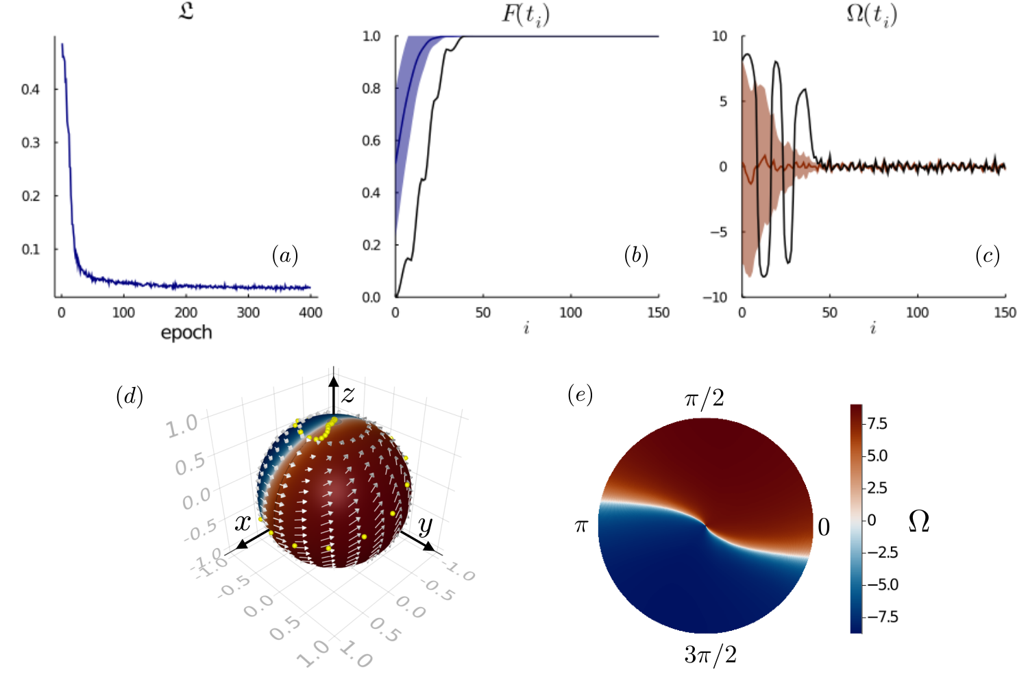
C.2 Technical details of the continuous adjoint sensitivity method for SDEs
To generalize the continuous adjoint sensitivity method for ODEs to Itô SDEs, one first needs to figure out how the sample path of an SDE can be reversed, i.e. how one can reconstruct the forward pass of the state from time to by a reversed time evolution from to launched at . The reversion of an SDE
| (71) |
defined in the Stratonovich sense, is given by [52, 53]
| (72) |
with noise values identical to those sampled in the forward pass. This closely resembles the reversion in case of an ODE shown in Eq. (68). To restore the noise, we use a dense noise grid of the noise values used in the forward pass. The memory overhead caused by using a noise grid could be traded against speed by using a virtual Brownian tree [52] or a Brownian interval [53], which enable the reconstruction of by storing only very little information such as the seed of the employed pseudo-random number generator. Despite the allocation of the noise values, the continuous stochastic adjoint sensitivity method is still much more memory efficient than a discrete reverse-mode AD backpropagation through the solver operations.
From the reverse Stratonovich SDE, Eq. (72), we can straightforwardly obtain the reverse Itô SDE
| (73) |
of the monitored qubit, Eq. (8), where the standard conversion rule
| (74) |
in Eq. (73) accounts for the required transformation from Itô to the Stratonovich sense and vice versa [54].
Analogously to the ODE case, taking the scalar loss function , Eq. (12), the adjoint process
| (75) |
to compute the gradients of with respect to the state is now a strong solution [54] of the adjoint Itô SDE
| (76) |
with the initial condition
| (77) |
Again, the value of the state of the forward pass is seen to be embedded in the vector-Jacobian products within the backward pass and, therefore, the knowledge of the state along its trajectory is necessary. Using Equation (73), we can recompute the state without having to store the full trajectory of the forward pass.
This SDE can be augmented by the additional quantity to compute the gradients . It is the solution of the stochastic differential equation
| (78) |
with the initial condition
| (79) |
As a consequence of the scalar noise character of the forward SDE, Eq. (8), the adjoint SDE with an augmented state according to Eqs. (73), (76), and (78) also has scalar noise. Similar to the ODE setting, solving SDEs backwards is not guaranteed to be stable. Thus, to improve the stability, we modify this approach by resetting the reverse integration using the checkpoints .
Appendix D The effect of the decay rate on the fidelity
In the main text, we report mean fidelities of about averaged over the whole control interval including the very low fidelities due to the transient initial dynamics. This value of the fidelity is determined by the physical parameters of the quantum system (, ) as well as by the experimental limitations of the control scheme (e.g. and the feedback control frequency). We note that these parameters are setup-specific and do not represent a hard fidelity limit for our proposed control scheme. In Figure 8, we demonstrate that the mean fidelity over the full time interval as well as the final state infidelity can easily be improved by decreasing the decay rate with respect to the detuning . In the limit , one recovers a fidelity close to unity comparable to the closed-system case, see C.1. We further see that the difference between the trained NN and the hand-crafted strategy gets more pronounced as is decreased.
References
References
- [1] D. D’Alessandro, Introduction to quantum control and dynamics. Chapman & Hall/CRC, 2008.
- [2] H. M. Wiseman and G. J. Milburn, Quantum measurement and control. Cambridge University Press, 2009.
- [3] S. J. Glaser, U. Boscain, T. Calarco, C. P. Koch, W. Köckenberger, R. Kosloff, I. Kuprov, B. Luy, S. Schirmer, T. Schulte-Herbrüggen, et al., “Training Schrödinger’s cat: quantum optimal control,” The European Physical Journal D, vol. 69, no. 12, pp. 1–24, 2015.
- [4] J. Zhang, Y. xi Liu, R.-B. Wu, K. Jacobs, and F. Nori, “Quantum feedback: Theory, experiments, and applications,” Physics Reports, vol. 679, pp. 1 – 60, 2017.
- [5] R. S. Sutton and A. G. Barto, Reinforcement Learning: An Introduction. The MIT Press, second ed., 2018.
- [6] T. P. Lillicrap, J. J. Hunt, A. Pritzel, N. Heess, T. Erez, Y. Tassa, D. Silver, and D. Wierstra, “Continuous control with deep reinforcement learning,” in International Conference on Learning Representations (Poster), 2016.
- [7] M. Y. Niu, S. Boixo, V. N. Smelyanskiy, and H. Neven, “Universal quantum control through deep reinforcement learning,” npj Quantum Information, vol. 5, no. 1, p. 33, 2019.
- [8] M. Bukov, “Reinforcement learning for autonomous preparation of Floquet-engineered states: Inverting the quantum Kapitza oscillator,” Physical Review B, vol. 98, p. 224305, Dec 2018.
- [9] M. Bukov, A. G. R. Day, D. Sels, P. Weinberg, A. Polkovnikov, and P. Mehta, “Reinforcement learning in different phases of quantum control,” Physical Review X, vol. 8, p. 031086, Sep 2018.
- [10] F. Schäfer, M. Kloc, C. Bruder, and N. Lörch, “A differentiable programming method for quantum control,” Machine Learning: Science and Technology, vol. 1, p. 035009, 2020.
- [11] C. Rackauckas, Y. Ma, J. Martensen, C. Warner, K. Zubov, R. Supekar, D. Skinner, and A. Ramadhan, “Universal differential equations for scientific machine learning,” arXiv preprint arXiv:2001.04385, 2020.
- [12] N. Leung, M. Abdelhafez, J. Koch, and D. Schuster, “Speedup for quantum optimal control from automatic differentiation based on graphics processing units,” Physical Review A, vol. 95, p. 042318, Apr 2017.
- [13] M. Abdelhafez, D. I. Schuster, and J. Koch, “Gradient-based optimal control of open quantum systems using quantum trajectories and automatic differentiation,” Physical Review A, vol. 99, p. 052327, May 2019.
- [14] C. Rackauckas, A. Edelman, K. Fischer, M. Innes, E. Saba, V. B. Shah, and W. Tebbutt, “Generalized physics-informed learning through language-wide differentiable programming.,” in AAAI Spring Symposium: MLPS, 2020.
- [15] H.-J. Liao, J.-G. Liu, L. Wang, and T. Xiang, “Differentiable programming tensor networks,” Physical Review X, vol. 9, p. 031041, 2019.
- [16] C. Rackauckas, M. Innes, Y. Ma, J. Bettencourt, L. White, and V. Dixit, “Diffeqflux.jl – a Julia library for neural differential equations,” arXiv preprint arXiv:1902.02376, 2019.
- [17] R.-B. Wu, H. Ding, D. Dong, and X. Wang, “Learning robust and high-precision quantum controls,” Physical Review A, vol. 99, p. 042327, Apr 2019.
- [18] L. Coopmans, D. Luo, G. Kells, B. K. Clark, and J. Carrasquilla, “Protocol Discovery for the Quantum Control of Majoranas by Differential Programming and Natural Evolution Strategies,” arXiv preprint arXiv:2008.09128, 2020.
- [19] H.-P. Breuer and F. Petruccione, The theory of open quantum systems. Oxford University Press, 2002.
- [20] T. Briant, P. Cohadon, M. Pinard, and A. Heidmann, “Optical phase-space reconstruction of mirror motion at the attometer level,” The European Physical Journal D - Atomic, Molecular, Optical and Plasma Physics, vol. 22, pp. 131–140, Jan 2003.
- [21] K. Iwasawa, K. Makino, H. Yonezawa, M. Tsang, A. Davidovic, E. Huntington, and A. Furusawa, “Quantum-limited mirror-motion estimation,” Phys. Rev. Lett., vol. 111, p. 163602, Oct 2013.
- [22] W. Wieczorek, S. G. Hofer, J. Hoelscher-Obermaier, R. Riedinger, K. Hammerer, and M. Aspelmeyer, “Optimal state estimation for cavity optomechanical systems,” Phys. Rev. Lett., vol. 114, p. 223601, Jun 2015.
- [23] H. M. Wiseman and G. J. Milburn, “Quantum theory of optical feedback via homodyne detection,” Phys. Rev. Lett., vol. 70, pp. 548–551, Feb 1993.
- [24] S. Mancini, D. Vitali, and P. Tombesi, “Optomechanical cooling of a macroscopic oscillator by homodyne feedback,” Phys. Rev. Lett., vol. 80, pp. 688–691, Jan 1998.
- [25] H. F. Hofmann, G. Mahler, and O. Hess, “Quantum control of atomic systems by homodyne detection and feedback,” Phys. Rev. A, vol. 57, pp. 4877–4888, Jun 1998.
- [26] A. C. Doherty and K. Jacobs, “Feedback control of quantum systems using continuous state estimation,” Phys. Rev. A, vol. 60, pp. 2700–2711, Oct 1999.
- [27] D. J. Wilson, V. Sudhir, N. Piro, R. Schilling, A. Ghadimi, and T. J. Kippenberg, “Measurement-based control of a mechanical oscillator at its themal decoherence rate,” Nature, vol. 524, p. 325, 2015.
- [28] H. Nha and H. J. Carmichael, “Entanglement within the quantum trajectory description of open quantum systems,” Phys. Rev. Lett., vol. 93, p. 120408, Sep 2004.
- [29] C. Viviescas, I. Guevara, A. R. R. Carvalho, M. Busse, and A. Buchleitner, “Entanglement dynamics in open two-qubit systems via diffusive quantum trajectories,” Phys. Rev. Lett., vol. 105, p. 210502, Nov 2010.
- [30] M. Koppenhöfer, C. Bruder, and N. Lörch, “Unraveling nonclassicality in the optomechanical instability,” Phys. Rev. A, vol. 97, p. 063812, Jun 2018.
- [31] M. Koppenhöfer, C. Bruder, and N. Lörch, “Heralded dissipative preparation of nonclassical states in a Kerr oscillator,” Phys. Rev. Research, vol. 2, p. 013071, Jan 2020.
- [32] S. Bose, P. L. Knight, M. B. Plenio, and V. Vedral, “Proposal for teleportation of an atomic state via cavity decay,” Phys. Rev. Lett., vol. 83, pp. 5158–5161, Dec 1999.
- [33] E. Greplova, K. Mølmer, and C. K. Andersen, “Quantum teleportation with continuous measurements,” Phys. Rev. A, vol. 94, p. 042334, Oct 2016.
- [34] Q. Ficheux, S. Jezouin, Z. Leghtas, and B. Huard, “Dynamics of a qubit while simultaneously monitoring its relaxation and dephasing,” Nature communications, vol. 9, no. 1, p. 1926, 2018.
- [35] R. Vijay, C. Macklin, D. Slichter, S. Weber, K. Murch, R. Naik, A. N. Korotkov, and I. Siddiqi, “Stabilizing Rabi oscillations in a superconducting qubit using quantum feedback,” Nature, vol. 490, no. 7418, pp. 77–80, 2012.
- [36] M. A. Armen, J. K. Au, J. K. Stockton, A. C. Doherty, and H. Mabuchi, “Adaptive homodyne measurement of optical phase,” Phys. Rev. Lett., vol. 89, p. 133602, Sep 2002.
- [37] M. Naghiloo, N. Foroozani, D. Tan, A. Jadbabaie, and K. Murch, “Mapping quantum state dynamics in spontaneous emission,” Nature communications, vol. 7, no. 1, pp. 1–7, 2016.
- [38] L. Bouten, R. Van Handel, and M. R. James, “An introduction to quantum filtering,” SIAM Journal on Control and Optimization, vol. 46, no. 6, pp. 2199–2241, 2007.
- [39] E. Flurin, L. S. Martin, S. Hacohen-Gourgy, and I. Siddiqi, “Using a recurrent neural network to reconstruct quantum dynamics of a superconducting qubit from physical observations,” Phys. Rev. X, vol. 10, p. 011006, Jan 2020.
- [40] C. Rackauckas and Q. Nie, “Differentialequations.jl–a performant and feature-rich ecosystem for solving differential equations in julia,” Journal of Open Research Software, vol. 5, no. 1, 2017.
- [41] C. Rackauckas and Q. Nie, “Adaptive methods for stochastic differential equations via natural embeddings and rejection sampling with memory,” Discrete and continuous dynamical systems. Series B, vol. 22, no. 7, p. 2731, 2017.
- [42] C. Rackauckas and Q. Nie, “Stability-optimized high order methods and stiffness detection for pathwise stiff stochastic differential equations,” in 2020 IEEE High Performance Extreme Computing Conference (HPEC), pp. 1–8, IEEE, 2020.
- [43] T. Caneva, T. Calarco, and S. Montangero, “Chopped random-basis quantum optimization,” Physical Review A, vol. 84, no. 2, p. 022326, 2011.
- [44] P. W. Glynn, “Likelihood ratio gradient estimation for stochastic systems,” Communications of the ACM, vol. 33, no. 10, pp. 75–84, 1990.
- [45] J. Yang and H. J. Kushner, “A Monte Carlo method for sensitivity analysis and parametric optimization of nonlinear stochastic systems,” SIAM journal on control and optimization, vol. 29, no. 5, pp. 1216–1249, 1991.
- [46] J. P. Kleijnen and R. Y. Rubinstein, “Optimization and sensitivity analysis of computer simulation models by the score function method,” European Journal of Operational Research, vol. 88, no. 3, pp. 413–427, 1996.
- [47] R. J. Williams, “Simple statistical gradient-following algorithms for connectionist reinforcement learning,” Machine learning, vol. 8, no. 3-4, pp. 229–256, 1992.
- [48] A. G. Baydin, B. A. Pearlmutter, A. A. Radul, and J. M. Siskind, “Automatic differentiation in machine learning: a survey,” The Journal of Machine Learning Research, vol. 18, no. 1, pp. 5595–5637, 2017.
- [49] R. E. Wengert, “A simple automatic derivative evaluation program,” Communications of the ACM, vol. 7, no. 8, pp. 463–464, 1964.
- [50] C. Rackauckas, Y. Ma, V. Dixit, X. Guo, M. Innes, J. Revels, J. Nyberg, and V. Ivaturi, “A comparison of automatic differentiation and continuous sensitivity analysis for derivatives of differential equation solutions,” arXiv preprint arXiv:1812.01892, 2018.
- [51] L. S. Pontryagin, Mathematical theory of optimal processes. Routledge, 2018.
- [52] X. Li, T.-K. L. Wong, R. T. Chen, and D. Duvenaud, “Scalable gradients for stochastic differential equations,” arXiv:2001.01328, 2020.
- [53] Anonymous, “Neural SDEs made easy: SDEs are infinite-dimensional GANs,” in Submitted to International Conference on Learning Representations, 2021. under review.
- [54] P. E. Kloeden and E. Platen, Numerical solution of stochastic differential equations. Springer Science & Business Media, 2013.
- [55] F. Schäfer, “High weak order solvers and adjoint sensitivity analysis for stochastic differential equations.” https://summerofcode.withgoogle.com/archive/2020/projects/5076877036748800/, 2020. [Online; accessed 15-February-2021].
- [56] J. Bezanson, S. Karpinski, V. B. Shah, and A. Edelman, “Julia: A fast dynamic language for technical computing,” arXiv preprint arXiv:1209.5145, 2012.
- [57] F. van der Meulen and M. Schauer, “Continuous-discrete smoothing of diffusions,” arXiv preprint arXiv:1712.03807, 2017.
- [58] F. van der Meulen and M. Schauer, “Automatic backward filtering forward guiding for markov processes and graphical models,” arXiv preprint arXiv:2010.03509, 2020.
- [59] J. Gough, V. P. Belavkin, and O. G. Smolyanov, “Hamilton–Jacobi–Bellman equations for quantum optimal feedback control,” Journal of Optics B: Quantum and Semiclassical Optics, vol. 7, no. 10, pp. S237–S244, 2005.
- [60] J. Sirignano and K. Spiliopoulos, “DGM: A deep learning algorithm for solving partial differential equations,” Journal of computational physics, vol. 375, pp. 1339–1364, 2018.
- [61] A. R. Gerlach, A. Leonard, J. Rogers, and C. Rackauckas, “The Koopman expectation: An operator theoretic method for efficient analysis and optimization of uncertain hybrid dynamical systems,” arXiv preprint arXiv:2008.08737, 2020.
- [62] A. Lamperski, K. R. Ghusinga, and A. Singh, “Analysis and control of stochastic systems using semidefinite programming over moments,” IEEE Transactions on Automatic Control, vol. 64, no. 4, pp. 1726–1731, 2018.
- [63] E. Greplova, C. K. Andersen, and K. Mølmer, “Quantum parameter estimation with a neural network,” arXiv preprint arXiv:1711.05238, 2017.
- [64] A. Valenti, E. van Nieuwenburg, S. Huber, and E. Greplova, “Hamiltonian learning for quantum error correction,” Physical Review Research, vol. 1, no. 3, p. 033092, 2019.
- [65] S. Krastanov, S. Zhou, S. T. Flammia, and L. Jiang, “Stochastic estimation of dynamical variables,” Quantum Science and Technology, vol. 4, no. 3, p. 035003, 2019.
- [66] F. Schäfer, P. Sekatski, M. Koppenhöfer, C. Bruder, and M. Kloc, “Control of Stochastic Quantum Dynamics with Differentiable Programming.” https://github.com/frankschae/Control-of-Stochastic-Quantum-Dynamics-with-Differentiable-Programming, 2021. [Online; accessed 15-February-2021].
- [67] S. L. Brunton, J. L. Proctor, and J. N. Kutz, “Discovering governing equations from data by sparse identification of nonlinear dynamical systems,” Proceedings of the National Academy of Sciences, vol. 113, no. 15, pp. 3932–3937, 2016.
- [68] L. Boninsegna, F. Nüske, and C. Clementi, “Sparse learning of stochastic dynamical equations,” The Journal of chemical physics, vol. 148, no. 24, p. 241723, 2018.
- [69] E. Kaiser, J. N. Kutz, and S. L. Brunton, “Sparse identification of nonlinear dynamics for model predictive control in the low-data limit,” Proceedings of the Royal Society A, vol. 474, no. 2219, p. 20180335, 2018.
- [70] M. Cranmer, A. Sanchez-Gonzalez, P. Battaglia, R. Xu, K. Cranmer, D. Spergel, and S. Ho, “Discovering symbolic models from deep learning with inductive biases,” NeurIPS 2020, 2020.
- [71] M. Innes, A. Edelman, K. Fischer, C. Rackauckus, E. Saba, V. B. Shah, and W. Tebbutt, “Zygote: A differentiable programming system to bridge machine learning and scientific computing.” arXiv preprint arXiv:1907.07587, 2019.
- [72] R. T. Chen, Y. Rubanova, J. Bettencourt, and D. K. Duvenaud, “Neural ordinary differential equations,” in Advances in neural information processing systems, pp. 6571–6583, 2018.
- [73] S. G. Johnson, “Notes on adjoint methods for 18.336,” 2007.
- [74] J. Jia and A. R. Benson, “Neural jump stochastic differential equations,” in Advances in Neural Information Processing Systems, pp. 9847–9858, 2019.