Iterated numerical homogenization for multi-scale elliptic equations with monotone nonlinearity

Xinliang Liu Note: liuxinliang@sjtu.edu.cn Institute of Natural Sciences, School of Mathematical Sciences, and MOE-LSC, Shanghai Jiao Tong University.
Eric Chung Note: tschung@math.cuhk.edu.hk Department of Mathematics, The Chinese University of Hong Kong, Shatin, Hong Kong. and Lei Zhang Note: lzhang2012@sjtu.edu.cn Institute of Natural Sciences, School of Mathematical Sciences, and MOE-LSC, Shanghai Jiao Tong University.

Abstract

Nonlinear multi-scale problems are ubiquitous in materials science and biology. Complicated interactions between nonlinearities and (nonseparable) multiple scales pose a major challenge for analysis and simulation. In this paper, we study the numerical homogenization for multi-scale elliptic PDEs with monotone nonlinearity, in particular the Leray-Lions problem (a prototypical example is the p-Laplacian equation), where the nonlinearity cannot be parameterized with low dimensional parameters, and the linearization error is non-negligible. We develop the iterated numerical homogenization scheme by combining numerical homogenization methods for linear equations, and the so-called ”quasi-norm” based iterative approach for monotone nonlinear equation. We propose a residual regularized nonlinear iterative method, and in addition, develop the sparse updating method for the efficient update of coarse spaces. A number of numerical results are presented to complement the analysis and valid the numerical method.

Keywords: numerical homogenization, multi-scale elliptic problem, monotone nonlinearity, $p$ -Laplacian, regularization, sparse updating.

1 Introduction

Problems with a wide range of coupled temporal and spatial scales are ubiquitous in many phenomena and processes of materials science and biology. Multi-scale modeling and simulation is essential in underpinning the discovery and synthesis of new materials and chemicals with novel functionalities in key areas such as energy, information technology and bio-medicine. In particular, for nonlinear multi-scale problems such as liver surgery, tissue growth, crack propagation, phase transformations, etc. [16, 66, 12, 44], complicated interactions between nonlinearity and (nonseparable) multiple scales pose a major challenge for the design and analysis of efficient and robust multi-scale numerical methods.

In this paper, we discuss the design, analysis and implementation of numerical homogenization type multi-scale methods for multi-scale elliptic PDEs with monotone nonlinearity. Let $\Omega\subset\mathbb{R}^{d}$ , $d\geqslant 2$ , be a polygonal (polyhedral) domain (open, bounded and connected), we consider the following nonlinear elliptic problem: find $u:\Omega\to\mathbb{R}$ , such that

\left\{\begin{aligned} -\nabla\cdot a(x,u(x),\nabla u(x))=f\quad\text{in }\Omega\\ u=0\quad\text{on }\partial\Omega\end{aligned}\right.

(1)

where $a(x,u(x),\nabla u(x)):\Omega\times\mathbb{R}\times\mathbb{R}^{d}\to\mathbb{R}^{d}$ is the nonlinear flux function, and $f:\Omega\to\mathbb{R}$ is the source term. The nonlinear flux function $a$ takes the general form $a(x,v,\bm{\xi})=A(x,v,\bm{\xi})\bm{\xi}$ for $(x,v,\bm{\xi})\in\Omega\times\mathbb{R}\times\mathbb{R}^{d}$ , where $A:\Omega\times\mathbb{R}\times\mathbb{R}^{d}\to\mathbb{R}^{d\times d}$ is a matrix-valued Carathéodory function (measurable in $x$ , continuous in $v$ and $\bm{\xi}$ ).

We will focus on the Leray-Lions type problem [53] such that $A(x,v,\bm{\xi})=A(x,\bm{\xi})$ for $(x,\bm{\xi})\in\Omega\times\mathbb{R}^{d}$ . This situation is very different from the quasilinear case where $A(x,v,\bm{\xi})=A(x,v)$ . In the quasilinear case, the nonlinearities within coarse regions, that induce the change in the heterogeneities, can be parametrized with a low dimensional parameter and linear multiscale theories can apply. For the Leray-Lions case, $\nabla u$ can be highly heterogeneous and one can not use any low dimensional approximation and linear theories. This is true even for a separable case $A(x,u,\nabla u)=\kappa(x)b(\nabla u)$ , which require nonlinear cell problems.

We assume that the Leray-Lions flux takes the following heterogeneous $\varphi$ -Laplacian form: $a(x,\bm{\xi})=\kappa(x)\varphi^{\prime}(|\bm{\xi}|)\bm{\xi}/|\bm{\xi}|$ , for $(x,\bm{\xi})\in\Omega\times\mathbb{R}^{d}$ [29]. $\kappa(\bm{x})\in L^{\infty}(\Omega)$ is symmetric, uniformly elliptic on $\Omega$ , and may contain (non-separable) multiple scales. If $\varphi\in C^{2}:\mathbb{R}^{+}\to\mathbb{R}^{+}$ is the so-called $N-$ function [29] (see also Section 2.1), where the well-know p-Laplacian is a special case such that $\varphi(t)=t^{p}/p$ for $p>1$ , the nonlinear multi-scale problem (1) admits a natural variational form (2), and also admits a unique solution in the Orlicz-Sobolev space $V:=W_{0}^{1,\varphi}(\Omega)$ [29] ( $W_{0}^{1,p}$ for the p-Laplacian case). More general nonlinear flux will be treated in our future work. The heterogeneous $\varphi$ -Laplacian model have applications in many areas such as nonlinear materials [44], non-Newtonian fluids [27], image processing [42], machine learning [68], etc.

There are various numerical homogenization approaches for linear multi-scale problems, such as homogenization [65, 50], numerical homogenization [30, 2, 69], heterogeneous multi-scale methods [31, 1, 57], multi-scale network approximations [7], multi-scale finite element methods [4, 36, 37, 33], variational multi-scale methods [49, 6], flux norm homogenization [8, 61], rough polyharmonic splines (RPS) [63], generalized multi-scale finite element methods [34, 20, 22]. In this paper, we will use the so-called RPS [63] or GRPS (generalized rough polyharmonic splines) method as a representative method.

Some of those ideas can be extended to nonlinear problems [43, 44, 38, 35, 23]. These approaches approximate the solution of nonlinear PDEs on a coarse grid (see Figure 4 for an illustration of coarse and fine grids) by using subgrid models. Some common ingredients in these methods are that local solutions are pre-computed over coarse patches, and coarse solves are performed over the coarse space spanned by those bases. The extensions of these methods to nonlinear problems use nonlinear local problems. For example, for the Leray-Lions flux $a(x,\nabla u)$ , one can use a local problem to compute a basis $\phi$ in each coarse cell, such that $-\mbox{div}(a(x,\nabla\phi_{\xi}))=0$ , with boundary conditions $\phi=\xi\cdot x$ . The homogenized fluxes are computed by averaging the flux $a^{*}(\xi)=\langle a(x,\nabla\phi_{\xi})\rangle$ . These approaches follow homogenization theory ([39, 64, 47, 46, 15, 3, 54, 58], see also [1, 47, 57] and, the references therein, for numerical homogenization. Also, Desbrun et. al. have applied ideas from linear numerical homogenization to coarse graining and model reduction of heterogeneous and nonlinear elasticity problems, as well as Navier-Stokes equations [51, 13, 10, 14].

For linear problems, one can construct one linear basis function per coarse node that contains the effects of small scales, in contrast, for nonlinear problems, one may need more multi-scale basis functions for each coarse cell. In [40, 18], the authors developed a systematic enrichment method, which calculates multi-scale basis functions via local spectral decomposition in each coarse cell, combined with nonlinear harmonic extensions, in order to capture small scales. The approach guarantees the recovery of homogenization results when there is a scale separation, and it is in a spirit of hybridization techniques [24, 41, 17].

In this paper, we take an alternative view for the numerical homogenization of nonlinear elliptic problems. Our view is based on the well-established fact that linear multi-scale problem can be well approximated by the coarse space up to the coarse resolution, even with nonseparable scales. Therefore, our goal is to find a sequence of approximate linear problems and the corresponding coarse spaces, which we call iterated numerical homogenization, for the original nonlinear problem. We first present an idealized construction using the so-called ”quasi-norm” [26, 27] and prove the exponential energy convergence of this approach, which is independent of the heterogeneity. Although the resulting numerical scheme is implicit, we can interpret the preconditioned gradient descent method and Newton’s method as explicit relaxations of the quasi-norm approach, and show similar exponential energy convergence up to some reasonable assumptions. Although we do not need multiple basis functions per coarse node, we update the coarse space at each iteration. Therefore, we propose a sparse updating strategy to compute only a fraction of basis functions per iteration.

The paper is organized as follows. In Section 2, we present the abstract setting of the nonlinear problem and its regularization, also the finite element formulation and the numerical homogenization for linear problem. The iterative method, and the iterated numerical homogenization are formulated and analyzed in Section 3. We present numerical experiments to validate the methods in Section 4, and conclude the paper in Section 5.

Notations: The symbol $C$ (or $c$ ) denotes generic positive constant that may change from one line of an estimate to the next. The dependence of $C$ will be clear from the context or stated explicitly. To further simplify notation we will often write $\lesssim$ to mean $\leqslant C$ as well as $\eqsim$ to mean both $\lesssim$ and $\gtrsim$ . We use the standard definitions and notations $L^{p}$ , $W^{k,p}$ , $H^{k}$ for Lebesgue and Sobolev spaces. We denote the open ball with radius $r$ about $x$ and $0$ by $B_{r}(x)$ and $B_{r}:=B_{r}(0)$ .

2 Preliminaries

We briefly describe some preliminary knowledge needed in the paper. We first introduce the weak formulation and N-functions for the monotone nonlinear elliptic problem. We then discuss the regularization of the possible degeneracy/singularity, which can be used to guarantee the well-posedness of linearized problems. In the end, we formulate the finite element method for the nonlinear problem, and also the numerical homogenization for linear problems.

2.1 Weak Formulation and N-function

We define the following energy functional

\mathcal{J}(u):=\int_{\Omega}\kappa(x)\varphi(|\nabla u|)-\int_{\Omega}fu,\quad u\in V,

(2)

where $\Omega$ is a bounded open set in $\mathbb{R}^{d}$ with piecewise Lipschitz boundary $\partial\Omega$ . $\kappa_{\max}\geqslant\kappa(x)\geqslant\kappa_{\min}>0$ , $\kappa(x)$ is a heterogeneous coefficient with oscillations and possible high contrast, i.e., $\kappa_{\max}/\kappa_{\min}$ is large. In this paper, we assume that the forcing term $f\in L^{2}(\Omega)$ , unless otherwise specified. It is well known that the variational problem: Find $u\in V$ , such that

u=\argmin_{v\in V}\mathcal{J}(v)

(3)

is equivalent to the weak form of nonlinear elliptic equation (1): Find $u\in V$ , such that

\langle Au,v\rangle=\int_{\Omega}a(x,\nabla u)\cdot\nabla v=\int_{\Omega}fv,\quad\forall v\in V

(4)

where $a(x,\bm{\xi})=\kappa(x)\varphi^{\prime}(|\bm{\xi}|)\bm{\xi}/|\bm{\xi}|$ .

We introduce the so-called N-function, and associated function spaces. A continuous function $\varphi$ is said to be a N-function if the derivative $\varphi^{\prime}$ exists, and in addition, $\varphi^{\prime}$ has the following properties: right continuous, $\varphi^{\prime}(0)=0$ , $\varphi^{\prime}(t)>0$ for $t>0$ , and $\lim_{t\rightarrow\infty}\varphi^{\prime}(t)=\infty$ .

We denote $\mathcal{L}^{\varphi}(\Omega):=\left\{w:\Omega\rightarrow\mathbb{R}:w\text{ measurable and }\int_{\Omega}\varphi(|w|)dx<\infty\right\}$ as the classical Orlicz space, and we say $f\in W^{1,\varphi}$ , the Sobolev-Orlicz space, if and only if $f$ , $\nabla f\in L^{\varphi}$ . See Appendix A.2 for more details, such as the definition of the norms $\|\cdot\|_{L^{\varphi}}$ and $\|\cdot\|_{W^{1,\varphi}}$ . Let $V:=W^{1,\varphi}_{0}$ denote the Banach space endowed with $\|\cdot\|_{W^{1,\varphi}}$ and homogeneous boundary condition, and $V^{*}$ be its dual space with norm $\|\cdot\|_{W^{-1,\varphi}}$ . $V$ is a reflexive and separable Banach space. If $\varphi$ is a N-function and $f\in V^{*}$ , (3)/(4) is well-posed and admits a unique solution in $V$ .

We say that $\varphi$ satisfies the $\Delta_{2}$ -condition, if there exists $c>0$ such that for all $t\geqslant 0$ , it holds that $\varphi(2t)\leqslant c\varphi(t)$ , and we denote $\Delta_{2}(\varphi)$ as the smallest such constant $c$ . Since $\varphi(t)\leqslant\varphi(2t)$ , the $\Delta_{2}$ condition is equivalent to $\varphi(2t)\sim\varphi(t)$ . We define the function $(\varphi^{\prime})^{-1}:\mathbb{R}^{+}\to\mathbb{R}^{+}$ by $(\varphi^{\prime})^{-1}(t):=\sup\{u\in\mathbb{R}^{+}:\phi^{\prime}(u)\leqslant t\}$ . If $\varphi^{\prime}$ is strictly increasing then $(\varphi^{\prime})^{-1}$ is the inverse function of $\varphi^{\prime}$ . $\varphi^{*}:\mathbb{R}^{+}\to\mathbb{R}^{+}$ with $\varphi^{*}(t):=\int_{0}^{t}(\varphi^{\prime})^{-1}(s)\mathrm{ds}$ is again an N-function. $\varphi^{*}$ is the complementary function of $\varphi$ such that $(\varphi^{*})^{*}=\varphi$ . For any $a\geqslant 0$ , we define the shifted N-function by $\varphi_{a}^{\prime}(t):=\frac{\varphi^{\prime}(a\vee t)}{a\vee t}$ and $\varphi_{a}(t):=\int_{0}^{t}\varphi^{\prime}(s)ds$ .

Uniformly in $t\geqslant 0$ , we have $\varphi(t)\sim\varphi^{\prime}(t)t$ , where the constants depends only on $\Delta_{2}(\varphi,\varphi^{*}):=\max(\Delta_{2}(\varphi),\Delta_{2}(\varphi^{*}))$ . In addition, we make the following assumption,

Assumption 1 (N-function).

Let $\varphi$ be an N-function with strictly increasing $\varphi^{\prime}$ , and $\Delta_{2}(\{\varphi,\varphi^{*}\})<\infty$ . We assume that

1.

$\varphi^{\prime\prime}$ exists, is right continuous, and satisfies $\varphi^{\prime}(t)\sim t\varphi^{\prime\prime}(t)$ uniformly in $t\geqslant 0$ .
2.

$\varphi^{\prime\prime}$ is non-decreasing.

Remark 2.

Assumption 1 is satisfied by p-Laplacian $\varphi(t)=t^{p}/p$ for $p\geqslant 2$ , and also the regularized p-Laplacian defined in 2.2.

We have the following properties of the flux function associated with an N-function $\varphi$ .

Property 3.

For $a(x,\bm{\xi})=\kappa(x)\varphi^{\prime}(|\bm{\xi}|)\frac{\bm{\xi}}{|\bm{\xi}|}$ , and $\kappa(x)>0$ , it holds that

(1)

$(a(x,\bm{\xi})-a(x,\bm{\zeta}))\cdot(\bm{\xi}-\bm{\zeta})\geqslant c\kappa(x)\varphi^{\prime\prime}(|\bm{\xi}|+|\bm{\zeta}|)|\bm{\xi}-\bm{\zeta}|^{2}$ ,
(2)

$|a(x,\bm{\xi})-a(x,\bm{\zeta})|\leqslant C\kappa(x)\varphi^{\prime\prime}(|\bm{\xi}|+|\bm{\zeta}|)|\bm{\xi}-\bm{\zeta}|$ ,
(3)

$a(x,\bm{0})=0$ .

where $\varphi$ is an N-function, the constants $c,C$ only depends on $\Delta_{2}({\varphi,\varphi^{*}})<\infty$ .

Property 3 has been proved for p-Laplacian in [5, 32]. We will provide more properties of N-functions in the appendix A.1.

The functional $\mathcal{J}$ is strictly convex. Furthermore, $\mathcal{J}$ is differentiable and second order Gateaux differentiable. Formally, its first and second variation are given as follows

\mathcal{J}^{\prime}(u)(v)=\int_{\Omega}\kappa(x)\frac{\varphi^{\prime}(|\nabla u|)}{|\nabla u|}\nabla u\cdot\nabla v-\int_{\Omega}fv,

(5)

\mathcal{J}^{\prime\prime}(u)(v,w)=\int_{\Omega}\kappa(x)\frac{\varphi^{\prime}(|\nabla u|)}{|\nabla u|}\nabla v\cdot\nabla w+\int_{\Omega}\kappa(x)\frac{\varphi^{\prime\prime}(|\nabla u|)|\nabla u|-\varphi^{\prime}(|\nabla u|)}{|\nabla u|^{3}}(\nabla u\cdot\nabla w)(\nabla u\cdot\nabla v).

(6)

We define the Bregman distance [9] of $\mathcal{J}$ as

\mathcal{D}_{\mathcal{J}}(u,v):=\mathcal{J}(u)-\mathcal{J}(v)-\mathcal{J}^{\prime}(v)(u-v).

(7)

Lemma 4.

We assume that $\varphi$ satisfies Assumption 1. For any $u,v\in V$ , there exists constants $0<c_{\mathcal{J}}<C_{\mathcal{J}}$ , which depend on $\Delta_{2}(\varphi,\varphi^{*})$ , and are independent of $\kappa$ such that

c_{\mathcal{J}}\int\kappa(x)\varphi^{\prime\prime}(|\nabla u|+|\nabla(u-v)|)|\nabla(u-v)|^{2}\leqslant\mathcal{D}_{\mathcal{J}}(u,v)\leqslant C_{\mathcal{J}}\int\kappa(x)\varphi^{\prime\prime}(|\nabla u|+|\nabla(u-v)|)|\nabla(u-v)|^{2}

(8)

see A.3 for the proof.

The term $\int\kappa(x)\varphi^{\prime\prime}(|\nabla u|+|\nabla(u-v)|)|\nabla(u-v)|^{2}$ is called the quasi-norm associated with $\varphi$ , which has already been defined in [5, 32] for p-Laplacian equation.

Remark 5.

For $p$ -laplacian problem with $\varphi(t)=t^{p}/p$ with $p>1$ , we have

\mathcal{J}(u)=\frac{1}{p}\int_{\Omega}\kappa(x)|\nabla u|^{p}-\int_{\Omega}fu,\quad u\in V

(9)

where the Orlicz space $W^{1,\varphi}_{0}(\Omega)$ reduces to $W_{0}^{1,p}(\Omega)$ , and $f\in W^{-1,q}(\Omega)$ ( $1/p+1/q=1$ ).

\mathcal{J}^{\prime}(u)(v)=\int_{\Omega}\kappa(x)|\nabla u|^{p-2}\nabla u\cdot\nabla v-\int_{\Omega}fv.

(10)

\mathcal{J}^{\prime\prime}(u)(v,w)=\int_{\Omega}\kappa(x)|\nabla u|^{p-2}\nabla v\cdot\nabla w+(p-2)\int_{\Omega}\kappa(x)|\nabla u|^{p-4}(\nabla u\cdot\nabla v)(\nabla u\cdot\nabla w).

(11)

where $u,v,w\in V$ .

2.2 Regularization

Let $u\in W^{1,\varphi}_{0}$ be the solution of (3)/(4), $\kappa(x)\varphi^{\prime}(\nabla u)/|\nabla u|$ can be treated as the coefficient of the elliptic equation (4). It is possible that $u$ has critical points such that $|\nabla u|=0$ , also $\varphi^{\prime}(\nabla u)/|\nabla u|$ may grow large. The interaction between $\kappa(x)$ and nonlinearity may amplify such a degeneracy/singularity.

Regularization techniques have been developed in [25] for $1<p<2$ , and for optimal control problem governed by $p-$ Laplacian in [11]. We adapt those methods and propose a two parameter regularized energy functional $\mathcal{J}_{\epsilon}$ . Let regularization parameters be $\epsilon:=\{\epsilon_{-},\epsilon_{+}\}$ such that $0<\epsilon_{-}<\epsilon_{+}$ . We take $\varphi(t)=t^{p}/p$ as an example, and introduce a regularized N-function $\varphi_{\epsilon}:\mathbb{R}^{+}\longrightarrow\mathbb{R}$ , such that $\varphi(t)=\lim_{\epsilon\rightarrow\{0,\infty\}}\varphi_{\epsilon}(t)$ for all $t\geqslant 0$ and $\varphi_{\epsilon}(t)\approx\epsilon_{+/-}^{p-2}t^{2}$ for $t\geqslant\epsilon_{+}$ and $0\leqslant t\leqslant\epsilon_{-}$ . See (53) and (54) for two concrete examples. Notice that $\mathcal{J}_{\epsilon}(v)<\infty$ , if and only if $v\in$ $W_{0}^{1,2}(\Omega)$ .

We define the regularized energy functional as

\mathcal{J}_{\epsilon}(u)=\int_{\Omega}\kappa(x)\varphi_{\epsilon}(|\nabla u|)-\int_{\Omega}fu,\quad u\in H_{0}^{1}.

(12)

The regularization error in energy can be defined as,

\mathrm{err}^{\mathrm{reg}}:=\mathcal{J}(u)-\mathcal{J}_{\epsilon}(u_{\epsilon}),

(13)

where $u_{\epsilon}$ is the energy minimizer of $\mathcal{J}_{\epsilon}$ . It is beyond the scope of this work to investigate the decay of the regularization error with respect to the regularization parameters $\epsilon$ . Instead, we have the following Lemma 15 ([11, Lemma 5.2]) and make Assumption 16 for the regularization error.

Lemma 6.

$\mathcal{J}_{\epsilon}$ has a unique minimizer $u_{\epsilon}\in H^{1}_{0}$ for any $\{\epsilon_{-},\epsilon_{+}\}\subset(0,\infty)$ . Let the sequence $\{\epsilon_{-,k},\epsilon_{+,k}\}\longrightarrow\{0,\infty\}$ , we obtain a sequence of minimizers $u_{\epsilon_{k}}$ of the regularized variational problems. Let $u$ be the solution of (2). It holds true that

u_{\epsilon_{k}}\rightarrow u\quad in\quad H_{0}^{1}(\Omega),\quad\text{ as }k\rightarrow\infty,

(14)

\chi_{\Omega\backslash\Omega_{k}\left(u_{\epsilon_{k}}\right)}\nabla u_{\epsilon_{k}}\rightarrow\nabla u,\quad\text{ strongly in }L^{p}(\Omega)^{d}.

(15)

Assumption 7 (Regularization).

For some $q>p>0$ , we have

\mathrm{err}^{\mathrm{reg}}\sim{\epsilon_{-}}^{p}+{\epsilon_{+}}^{p-q}.

(16)

2.3 Finite Element Approximation

We set up the finite element approximation of the weak formulation (4). Let $\mathcal{T}_{H}$ be a coarse simplicial subdivision of $\Omega$ , with the coarse mesh size $H:=\max_{K\in\mathcal{T}_{H}}H_{K}$ , and $H_{K}:=\mathrm{diam}(K)$ . We assume that $\mathcal{T}_{H}$ is shape regular in the sense that $\max_{K\in\mathcal{T}_{H}}\frac{h_{K}}{\rho_{K}}\leqslant\gamma$ , for a positive constant $\gamma>0$ , where $\rho_{K}$ is the radius of the inscribed circle in $K$ . Let $\Omega_{i}^{0}$ be a coarse simplex, e.g. a coarse node $x_{i}$ or a coarse element $T_{i}$ , we define the $\ell$ -th layer patch $\Omega^{\ell}_{i}=\cup\{T\in\mathcal{T}_{H}:T\cap\Omega^{\ell-1}_{i}\neq\emptyset\}$ for $\ell\geqslant 1$ recursively. A fine mesh $\mathcal{T}_{h}$ with mesh size $h$ can be obtained by uniformly subdivide $\mathcal{T}_{H}$ several times. See Figures 4 and 5 for illustrations.

The finite element space $\mathcal{V}_{h}$ contains continuous piecewise linear functions with respect to $\mathcal{T}_{h}$ which vanish at the boundary $\partial\Omega$ . We only consider continuous piecewise linear functions since higher order regularity of $p$ -Laplacian problem is not guaranteed [55]. The discrete finite element problem is defined in the following: Find $u_{h}\in\mathcal{V}_{h}$ such that

\int_{\Omega}a(x,\nabla u_{h})\cdot\nabla v=\int_{\Omega}fv_{h},\qquad\forall v_{h}\in\mathcal{V}_{h}.

(17)

or equivalently

\min_{v_{h}\in\mathcal{V}_{h}}\mathcal{J}(v_{h})

(18)

By [28, 32], we have that $\|u-u_{h}\|\sim\epsilon(h)$ and

\mathrm{err}^{h}:=\mathcal{J}_{\epsilon}(u_{\epsilon})-\mathcal{J}_{\epsilon,h}(u_{\epsilon,h}),

(19)

such that $\epsilon(h)\to 0$ as $h\to 0$ . In this paper, we assume that the fine mesh error $\epsilon(h)$ is negligible.

2.4 Numerical Homogenization for Linear Elliptic Equation

For linear elliptic equation $-\mathrm{div}A(x)\nabla u=f$ with coefficient $A(x)\in(L^{\infty})^{d\times d}$ , $0<{m^{-}}:=\inf_{x\in\Omega}\lambda_{\min}(A(x))\leqslant\sup_{x\in\Omega}\lambda_{\max}(A(x))=:m^{+}$ . We call $m:=\{m^{-},m+\}$ the set of lower and upper bounds. The associated finite element formulation is

A(\nabla u_{h},\nabla v_{h})=(f,v_{h}),\qquad\forall v_{h}\in\mathcal{V}_{h}.

(20)

The goal of numerical homogenization is to identify a coarse space $\mathcal{V}_{H}$ , such that the coarse solution $u_{H}\in\mathcal{V}_{H}$ of

A(\nabla u_{H},\nabla v_{H})=(f,v_{H}),\qquad\forall v_{H}\in\mathcal{V}_{H}.

(21)

achieves (quasi-)optimal convergence rate, and also the construction of $\mathcal{V}_{H}$ achieves (quasi-)optimal complexity. By now, there have been a wide range of literatures on the numerical homogenization of linear elliptic operators, see [30, 2, 69, 31, 1, 57, 7, 4, 36, 37, 33, 49, 6, 8, 61, 63, 34, 20, 22] for an incomplete list of references. In the following, we briefly introduce the (generalized) rough polyharmonic splines (GRPS) [62, 56, 60], as a representative approach for the numerical homogenization of linear elliptic equation with coefficient $A(x)$ .

Given $N_{H}$ suitable measurement functions $\psi_{i}$ , $i=1,\dots,N_{H}$ , for example characteristic function of coarse patches, we define the spaces $\mathcal{V}_{i}:=\{\phi\in\mathcal{V}_{h}|\int_{\Omega}\phi(x)\psi_{j}(x)\mathrm{dx}=\delta_{i,j},j=1,\dots,N_{H}\}$ . The GRPS basis is given by the solution of the following constrained minimization problem which is strictly convex and admits a unique minimizer $\phi_{i}\in\mathcal{V}_{i}$ ,

\phi_{i}=\argmin\limits_{\phi\in\mathcal{V}_{i}}\|\phi\|_{,\Omega}^{2},

(22)

for an appropriate norm $\|\cdot\|_{,\Omega}$ , for example, the energy norm $\|\cdot\|_{A,\Omega}:=\int_{\Omega}A(x)|\nabla\cdot|^{2}\mathrm{dx}$ .

The GRPS approach naturally induces a two-level decomposition of $\mathcal{V}_{h}$ : We define the coarse space as $\mathcal{V}_{H}:={\rm span}\{\phi_{i}\}$ , and the fine space as $\mathcal{V}_{f}:=\{v\in\mathcal{V}_{h}|\int_{\Omega}\psi_{i}v\mathrm{dx}=0,i=1,\dots,N_{H}\}$ . Let $\langle\cdot,\cdot\rangle$ be the inner product induced by the norm $\|\cdot\|$ , then $\mathcal{V}_{H}\perp\mathcal{V}_{f}$ with respect to the $\langle\cdot,\cdot\rangle$ product. Furthermore, let $w_{\mathrm{I}}:=\sum_{i}(\int_{\Omega}\psi_{i}w\mathrm{dx})\phi_{i}(x)$ be the interpolation of $w\in\mathcal{V}_{h}$ in $\mathcal{V}_{H}$ , we have the optimal recovery property:

\|w\|^{2}=\|w_{\mathrm{I}}\|^{2}+\|w-w_{\mathrm{I}}\|^{2},

and the optimal approximation property of $\mathcal{V}_{H}$ ,

\|w-w_{\mathrm{I}}\|_{L^{2}(\Omega)}\leqslant C_{m}H\|w\|,

(23)

the constants $C_{m}$ depends on the bounds $m$ , the details of the proof can be found in [62, 60].

The basis in (22) has a global support, which can be localized to a small patch of size $O(H\log(1/H))$ , and still maintains the optimal accuracy of $O(H)$ . Let $\Omega^{\ell}_{i}$ be a $\ell$ -th layer coarse patch, we define the localized basis $\phi_{i}^{\ell}$ by the following constrained minimization problem,

\phi^{\ell}_{i}=\argmin\limits_{\phi\in\mathcal{V}_{i}\text{ and }\mathrm{supp}(\phi)\subset\Omega^{\ell}_{i}}\|\phi\|_{,\Omega^{\ell}_{i}}^{2},

(24)

Theorem 8.

We have the following properties of the localized basis,

1.

exponential decay of the truncation error:

$\|\phi_{i}-\phi^{\ell}_{i}\|\leqslant C\exp(-C^{\prime}\ell),$

where the constants $C$ , $C^{\prime}$ depend on $m$ .
2.

finite element error for the localized basis: if $\ell\simeq\log(1/H)$ , $u_{H}^{\ell}$ is the FEM solution of (21) in $\mathcal{V}_{H}^{\ell}:={\rm span}\{\phi_{i}^{\ell}\}$ , then

$\|u-u_{H}^{\ell}\|_{H^{1}(\Omega)}\leqslant CH\|f\|_{L^{2}(\Omega)}.$ (25)

Remark 9.

For the nonlinear problem (3), we can still define global or local variation basis as in (22) and (24). For example, the global basis can be defined by

\phi_{i}=\argmin\limits_{\phi\in W^{1,\varphi}(\Omega),(\phi,\psi_{j})=\delta_{ij}}\int_{\Omega}\kappa(x)\varphi(|\nabla\psi|)dx,

(26)

and it still decays exponentially. However, the basis does not have the optimal approximation property as in (23) due to the loss of orthogonality, see Figure 1.

Refer to caption — Figure 1: For the multiscale trigonometric example in 4.1, we solve (4) using the nonlinear basis defined in (26). The $H^{1}$ error does not converge with respect to the degrees of freedom.

3 Numerical Methods

We formulate the numerical methods in this section. For a nonlinear problem, we usually need to approximate the solution iteratively. We will first introduce an ‘ideal’ iterative method with exponential decay of energy error and convergence rate independent of the heterogeneity, which is based on the quasi-norm formulation. Next, we connect the widely used preconditioned gradient descent (PGD) and Newton’s method with the quasi-norm based approach, and show the exponential energy decay with some reasonable assumptions. As a consequence, we will formulate the iterated numerical homogenization method, and its $L^{2}$ residual regularization for the multiscale nonlinear equations.

3.1 Iterative Methods

3.1.1 Quasi-norm based Implicit Method

We formulate an ‘ideal’ iterative method based on the quasi-norm introduced in Lemma 4. Suppose that $u^{(n)}\in W^{1,\varphi}$ is the n-th iterative approximation to $u$ , and $w^{(n)}$ is an increment such that $u^{(n+1)}=u^{(n)}+w^{(n)}$ , which will be specified later.

By Lemma 4, for any $u^{(n)}$ and $w^{(n)}$ , we have

\mathcal{J}(u^{(n)}+w^{(n)})-\mathcal{J}(u^{(n)})\leqslant\mathcal{J}^{\prime}(u^{(n)})(w^{(n)})+C_{\mathcal{J}}\int_{\Omega}\kappa(x)\varphi^{\prime\prime}\left(|\nabla u^{(n)}|+|\nabla w^{(n)}|\right)|\nabla w^{(n)}|^{2}.

(27)

We can define the increment $w^{(n)}$ by

C_{q}\int_{\Omega}\kappa(x)\varphi^{\prime\prime}\left(|\nabla u^{(n)}|+|\nabla w^{(n)}|\right)\nabla w^{(n)}\cdot\nabla v=-\mathcal{J}^{\prime}(u^{(n)})(v),\,\forall v\in W^{1,\varphi},

(28)

where $C_{q}=C_{\mathcal{J}}+1$ , such that the following lemma holds.

Lemma 10.

Under Assumption 1, also assume that $u^{(n)}\in W_{0}^{1,\varphi}$ , there exists a unique $w^{(n)}\in W_{0}^{1,\varphi}$ satisfying (28). Furthermore, there exists a constant $C_{1}>1$ depending on $\varphi$ but independent of $\kappa$ , such that

\mathcal{J}(u^{(n)})-\mathcal{J}(u)\leqslant C_{1}\int_{\Omega}\kappa(x)\varphi^{\prime\prime}\left(|\nabla u^{(n)}|+|\nabla w^{(n)}|\right)|\nabla w^{(n)}|^{2},

(29)

and

\mathcal{J}(u^{(n)}+w^{(n)})-\mathcal{J}(u^{(n)})\leqslant-\int_{\Omega}\kappa(x)\varphi^{\prime\prime}\left(|\nabla u^{(n)}|+|\nabla w^{(n)}|\right)|\nabla w^{(n)}|^{2}.

(30)

See A.5 for proof.

Let the energy error be defined as

e^{(n)}:=\mathcal{J}(u^{(n)})-\mathcal{J}(u),

and we have the following theorem for its exponential decay.

Theorem 11.

For the direction $w^{(n)}$ defined in (28), let $u^{(n+1)}:=u^{(n)}+w^{(n)}$ , the energy error decays exponentially with

e^{(n+1)}\leqslant(1-\frac{1}{C_{1}})e^{(n)}

(31)

where $C_{1}$ only depends on $\Delta_{2}(\varphi,\varphi^{*})$ , and independent of $\kappa(x)$ .

Proof.

By lemma 10, we have

\mathcal{J}(u^{(n)})-\mathcal{J}(u^{(n+1)})\geqslant\frac{1}{C_{1}}(\mathcal{J}(u^{(n)})-\mathcal{J}(u))

(32)

which leads to the desired result.

3.1.2 Explicit Iterative Methods

The quasi-norm based iterative method has the exponential convergence for energy error, and the convergence rate is independent of the oscillatory coefficients $\kappa$ , by Theorem 11. However, at each iteration, the nonlinear equation (28) needs to be solved to find the search direction $w^{(n)}$ . Usually, we have to resort to some explicit iterative methods for $w^{(n)}$ in practice. This can be done, for example, by using a linearized/approximate operator $A[u^{(n)}]$ to find $w^{(n)}$ , and update $u^{(n+1)}=u^{(n)}+w^{(n)}$ .

To be more precise, we define the first variation of $\mathcal{J}$ at $u^{(n)}$ ,

\mathcal{J}^{\prime}(u^{(n)})(v)=\int_{\Omega}\kappa(x)\frac{\varphi^{\prime}(|\nabla u^{(n)}|)}{|\nabla u^{(n)}|}\nabla u^{(n)}\cdot\nabla v-\int_{\Omega}fv.

(33)

Let

A_{\mathrm{G}}[u^{(n)}](w^{(n)}_{\mathrm{G}},v):=\int_{\Omega}\kappa(x)\frac{\varphi^{\prime}(|\nabla u^{(n)}|)}{|\nabla u^{(n)}|}\nabla w^{(n)}_{\mathrm{G}}\cdot\nabla v,

(34)

be the linear operator corresponding to the preconditioned steepest descent method. For p-Laplacian it writes [48]

A_{\mathrm{G}}[u^{(n)}](w^{(n)}_{\mathrm{G}},v):=\int_{\Omega}\left(\kappa(x)\left|\nabla u^{(n)}\right|^{p-2}\right)\nabla w^{(n)}_{\mathrm{G}}\cdot\nabla v.

(35)

Also, let

	$\displaystyle A_{\mathrm{N}}[u^{(n)}](w^{(n)}_{\mathrm{N}},v):=$	$\displaystyle\int_{\Omega}\kappa(x)\frac{\varphi^{\prime}(\|\nabla u^{(n)}\|)}{\|\nabla u^{(n)}\|}\nabla w^{(n)}_{\mathrm{N}}\cdot\nabla v$		(36)
		$\displaystyle+\int_{\Omega}\kappa(x)\frac{\varphi^{\prime\prime}(\|\nabla u^{(n)}\|)\|\nabla u^{(n)}\|-\varphi^{\prime}(\|\nabla u^{(n)}\|)}{\|\nabla u^{(n)}\|^{3}}(\nabla u^{(n)}\cdot\nabla w^{(n)}_{\mathrm{N}})(\nabla u^{(n)}\cdot\nabla v),$		(36)

be the linear operator corresponding to the Newton’s method,

For $A[u^{(n)}]=A_{\mathrm{G}}[u^{(n)}]$ or $A[u^{(n)}]=A_{\mathrm{N}}[u^{(n)}]$ , the search direction $w^{(n)}$ is then defined analogous to (28), through the following equation,

C_{n}A[u^{(n)}](w^{(n)},v)=-\mathcal{J}^{\prime}(u^{(n)})(v),\text{ for }\forall v\in\mathcal{V}_{h}.

(37)

where $C_{n}$ is a scaling factor analogous to $C_{q}$ in (28).

We make the following assumption,

Assumption 12.

Assume that for $u^{(n)}\in H_{0}^{1}$ , there exists an unique $w^{(n)}\in H_{0}^{1}$ satisfying (37). Furthermore, There exists $C_{n}>0$ such that

C_{n}A[u^{(n)}](w^{(n)},w^{(n)})\geqslant(C_{\mathcal{J}}+1)\int_{\Omega}\kappa(x)\varphi^{\prime\prime}\left(|\nabla u^{(n)}|+|\nabla w^{(n)}|\right)|\nabla w^{(n)}|^{2}.

(38)

Remark 13.

For the well-posedness of (37) in $H^{1}_{0}$ , we need $A[u^{(n)}]$ is bounded from above and below. For example, we can regularize the operator $A[u^{(n)}]$ at each iteration, or alternatively, assume that we are solving a regularized variational problem as defined in 2.2 in the first place. In the latter case, the above assumption 38 can be satisfied uniformly by letting $C_{n}\simeq(\epsilon_{+}/\epsilon_{-})^{p-2}$ for any $u^{(n)},w^{(n)}\in H_{0}^{1}$ . For general $\varphi$ -Laplacian problems without regularization, (38) can only be satisfied for small $w^{(n)}$ , and the constant $C_{n}$ may depend on $u^{(n)}$ .

Lemma 14.

Under Assumptions 1 and 38, there exists a constant $C_{2}>1$ depending on $\Delta_{2}(\varphi)$ , $\Delta_{2}(\varphi^{*})$ , $C_{n}$ , but independent of $\kappa$ , such that

	$\displaystyle\mathcal{J}(u^{(n)})-\mathcal{J}(u)\leqslant C_{2}\int_{\Omega}\kappa(x)\varphi^{\prime\prime}\left(\|\nabla u^{(n)}\|+\|\nabla w^{(n)}\|\right)\|\nabla w^{(n)}\|^{2},$		(39)
	$\displaystyle\mathcal{J}(u^{(n)}+w^{(n)})-\mathcal{J}(u^{(n)})\leqslant-\int_{\Omega}\kappa(x)\varphi^{\prime\prime}\left(\|\nabla u^{(n)}\|+\|\nabla w^{(n)}\|\right)\|\nabla w^{(n)}\|^{2}.$		(40)

See A.5 for proof.

Theorem 15.

Under the conditions in Lemma 14, and furthermore we assume that $C_{n}$ in (37) is uniformly bounded, namely, $C_{n}\leqslant M_{C}$ , $\forall n\in\mathbb{N}$ . For the direction $w^{(n)}$ defined in (37), let $u^{(n+1)}:=u^{(n)}+w^{(n)}$ , there exists a constant $0<\theta<1$ such that

e^{(n+1)}\leqslant\theta e^{(n)},

(41)

where $\theta$ depends on $M_{C}$ , $\Delta_{2}(\varphi)$ , $\Delta_{2}(\varphi^{*})$ , and independent of $\kappa$ .

We can formulate the iterative algorithm here.

Algorithm 1 Iterative Methods

STEP 1: Initialize

u^{(0)}

n=0

, and tolerance

\varepsilon>0

. STEP 2: Find the increment

w^{(n)}

by solving (28) for the quasi-norm based approach, or (37) for either PGD direction with (34) or Newton’s direction with (36). STEP 3: Update

u^{(n+1)}:=u^{(n)}+w^{(n)}

.STEP 4: If

(\mathcal{J}(u^{(n)})-\mathcal{J}(u^{(n+1)}))/|\mathcal{J}(u^{(n)})|<\varepsilon

, STOP; else goto STEP 2 and set

n:=n+1

Remark 16.

In practice, the constants $C_{q}$ and $C_{n}$ are not known a priori. Instead, we can solve the equation

A[u^{(n)}](w^{(n)},v)=-\mathcal{J}^{\prime}(u^{(n)})(v),\text{ for }\forall v\in\mathcal{V}_{h},

(42)

and use a line search algorithm [59] to find $\alpha_{n}=\argmin_{\alpha\geqslant 0}\mathcal{J}(u^{(n)}+\alpha w^{(n)})$ , and update $u^{(n+1)}=u^{(n)}+\alpha_{n}w^{(n)}$ .

3.2 Iterated Numerical Homogenization

In Algorithm 1, each iteration requires solving elliptic type equation (37) which combines the highly oscillatory coefficient $\kappa(x)$ and the nonlinearity from $\varphi$ . Besides, the gradient $|\nabla u^{(n)}|$ may possibly approach zero or grow large during the iteration. Therefore, a proper multi-scale solver can be employed to reduce the computational cost and maintain the coarse mesh accuracy. We are going to iteratively use the numerical homogenization method introduced in Section 3.2 to solve (37).

Let the norm associated with $A[u^{(n)}]$ be $\|\cdot\|_{A[u^{(n)}]}$ , the corresponding coarse space basis $\phi^{(n)}_{i}$ can be defined by

\phi^{(n)}_{i}=\argmin\limits_{\phi\in\mathcal{V}_{i}}\|\phi\|_{A[u^{(n)}]}^{2},

(43)

and the coarse space $\mathcal{V}_{H}^{(n)}:=\mathrm{span}\{\phi^{(n)}_{i}\}$ .

We can find the search direction $w^{(n)}_{H}\in\mathcal{V}_{H}^{(n)}$ by solving (37) in $\mathcal{V}_{H}^{(n)}$ , with $A[u^{(n)}]$ given by (34) or (36).

C^{\prime}_{n}A[u^{(n)}](w^{(n)}_{H},v)=-\mathcal{J}^{\prime}(u^{(n)})(v),\quad\forall v\in\mathcal{V}_{H}^{(n)}.

(44)

Similar to Assumption 38, we make the following assumption,

Assumption 17.

There exists $C^{\prime}_{n}>0$ such that,

C^{\prime}_{n}A[u^{(n)}](w^{(n)}_{H},w^{(n)}_{H})\geqslant(C_{\mathcal{J}}+1)\int_{\Omega}\kappa(x)\varphi^{\prime\prime}\left(|\nabla u^{(n)}|+|\nabla w^{(n)}_{H}|\right)|\nabla w^{(n)}_{H}|^{2}.

(45)

For simplicity, we take $C^{\prime}_{n}=C_{n}$ in both (38) and (45). Please see Figure 9 for numerical results and discussions related to Assumptions 38 and 45.

Lemma 18.

Suppose that $u^{(n)}\in\mathcal{V}_{h}$ . There exists positive constants $C_{\mathcal{T}_{h}}$ depending on the shape regularity of the mesh $\mathcal{T}_{h}$ , such that,

\|\mathcal{J}^{\prime}(u^{(n)})\|_{L_{h}^{2}}\leqslant\frac{C_{\mathcal{T}_{h}}}{h}\|a(x,\nabla u^{(n)})\|_{L^{2}}+\|f\|_{L^{2}},

(46)

where $\|\mathcal{J}^{\prime}(u^{(n)})\|_{L_{h}^{2}}$ is defined as $\|\mathcal{J}^{\prime}(u^{(n)})\|_{L_{h}^{2}}:=\displaystyle\min_{v_{h}\in\mathcal{V}_{h}}\frac{<\mathcal{J}^{\prime}(u^{(n)}),v_{h}>}{\|v_{h}\|_{L^{2}}}$

Proof.

The proof is based on the scaling argument that for any $v_{h}\in\mathcal{V}_{h}$ , $\|\nabla v_{h}\|_{L^{2}}\leqslant C_{\mathcal{T}_{h}}/h\|v_{h}\|_{L^{2}}$ , where the constant $C_{\mathcal{T}_{h}}$ depends only on the mesh regularity. Therefore, we have $\|\mathcal{J}^{\prime}(u^{(n)})\|_{L_{h}^{2}}\leqslant C_{\mathcal{T}_{h}}/h\|a(x,\nabla u^{(n)})\|_{L^{2}}+\|f\|_{L^{2}}$ .

Corollary 19.

For the finite element solution $w^{(n)}_{H}\in\mathcal{V}_{H}^{(n)}$ to (37), where $\mathcal{V}_{H}^{(n)}$ is the space of ”good” basis (global basis or local basis with $\ell\simeq\log H$ such that (25) holds). We have

\|w^{(n)}_{h}-w^{(n)}_{H}\|_{A[u^{(n)}]}\leqslant\frac{1}{C_{n}\lambda_{\min}(A[u^{(n)}])^{1/2}}H\|\mathcal{J}^{\prime}(u^{(n)})\|_{L_{h}^{2}}.

(47)

where $\lambda_{\min}(A[u^{(n)}]):=\inf_{x\in\Omega}\inf_{\|v\|=1}v^{T}a[u^{(n)}](x)v$ , and $a[u^{(n)}](x)$ denotes the elliptic coefficient in the operator $A[u^{(n)}]$ .

Theorem 20.

Under the conditions in Lemma 14, and furthermore we assume that $1\leqslant C_{n}\leqslant M_{C}$ , $\|\mathcal{J}^{\prime}(u^{(n)})\|_{L^{2}_{h}}^{2}\leqslant M_{L}$ , and $\lambda_{\min}(A[u^{(n)}])\geqslant M_{A}>0$ uniformly for $n\geqslant 0$ . For the direction $w^{(n)}_{H}$ defined in (44), and $u^{(n+1)}:=u^{(n)}+w^{(n)}_{H}$ , there exists a constant $C_{H}>0$ such that

(e^{(n+1)}-C_{H}H^{2})\leqslant(1-\frac{\theta}{C_{\mathcal{J}}+1})(e^{(n)}-C_{H}H^{2}),

(48)

where $C_{H}$ depends on $m$ , $\Delta_{2}(\varphi,\varphi^{*})$ , $M_{C}$ , $M_{L}$ and $M_{A}$ . $\theta$ is the constant in Theorem 15.

Proof.

By Assumption 45, we have

C_{n}A[u^{(n)}](w^{(n)}_{H},w^{(n)}_{H})\geqslant(C_{\mathcal{J}}+1)\int_{\Omega}\kappa(x)\varphi^{\prime\prime}\left(|\nabla u^{(n)}|+|\nabla w^{(n)}_{H}|\right)|\nabla w^{(n)}_{H}|^{2},

(49)

Combining Lemma 4, (44), (47), and (49), we derive the following inequalities,

	$\displaystyle\mathcal{J}(u^{(n)})-\mathcal{J}(u^{(n)}+w^{(n)}_{H})$	$\displaystyle\geqslant C_{n}A[u^{(n)}](w^{(n)}_{H},w^{(n)}_{H})-C_{\mathcal{J}}\int_{\Omega}\kappa(x)\varphi^{\prime\prime}\left(\|\nabla u^{(n)}\|+\|\nabla w^{(n)}_{H}\|\right)\|\nabla w^{(n)}_{H}\|^{2}$
		$\displaystyle\geqslant\frac{C_{n}}{C_{\mathcal{J}}+1}A[u^{(n)}](w^{(n)}_{H},w^{(n)}_{H})$
		$\displaystyle=\frac{C_{n}}{C_{\mathcal{J}}+1}A[u^{(n)}](w^{(n)}_{h},w^{(n)}_{h})+\frac{C_{n}}{C_{\mathcal{J}}+1}A[u^{(n)}](w^{(n)}_{h}-w^{(n)}_{H},w^{(n)}_{h}-w^{(n)}_{H})$
		$\displaystyle\geqslant\frac{C_{n}}{C_{\mathcal{J}}+1}A[u^{(n)}](w^{(n)}_{h},w^{(n)}_{h})-\frac{1}{(C_{\mathcal{J}}+1)C_{n}\lambda_{\min}(A[u^{(n)}])}\\|\mathcal{J}^{\prime}(u^{(n)})\\|_{L^{2}_{h}}^{2}H^{2}$
		$\displaystyle\geqslant\frac{1}{C_{\mathcal{J}}+1}(\mathcal{J}(u^{(n)})-\mathcal{J}(u^{(n)}+w^{(n)}_{h}))-\frac{M_{L}}{(C_{\mathcal{J}}+1)M_{A}}H^{2}.$

Let $e^{(n+1)}_{H}:=\mathcal{J}(u^{(n)}+w^{(n)}_{H})-\mathcal{J}(u)$ , and $\tilde{e}^{(n+1)}:=\mathcal{J}(u^{(n)}+w^{(n)}_{h})-\mathcal{J}(u)$ , by Theorem 15, we have

e^{(n)}_{H}-e^{(n+1)}_{H}\geqslant\frac{1}{C_{\mathcal{J}}+1}(e^{(n)}_{H}-\tilde{e}^{(n+1)})-\frac{M_{L}}{(C_{\mathcal{J}}+1)M_{A}}H^{2}\geqslant\frac{\theta}{C_{\mathcal{J}}+1}e^{(n)}_{H}-\frac{M_{L}}{(C_{\mathcal{J}}+1)M_{A}}H^{2}.

It follows by rearranging terms that,

(1-\frac{\theta}{C_{\mathcal{J}}+1})(e^{(n)}_{H}-\frac{M_{L}}{\theta M_{A}}H^{2})\geqslant(e^{(n+1)}_{H}-\frac{M_{L}}{\theta M_{A}}H^{2}),

namely, the energy error decays exponentially up to order $O(H^{2})$ , which concludes the theorem.

We summarize the iterated numerical homogenization method in the following algorithm.

Algorithm 2 Iterated Numerical Homogenization

STEP 1: Initialize

u^{(0)}

n=0

, and tolerance

\varepsilon>0

.STEP 2: Construct a coarse space

\mathcal{V}^{(n)}_{H}:={\rm span}\{\phi^{(n)}_{i},i=1,...,N_{H}\}

, where each

\phi^{(n)}_{i}

is obtained by solving the minimization problem (43) associated with the quadratic form

A[u^{(n)}]

.STEP 3: Find the search direction

w^{(n)}_{H}

by solving (44) for either the PGD direction in (34) or the Newton’s direction in (36).STEP 4: Update

u^{(n+1)}:=u^{(n)}+w^{(n)}_{H}

.STEP 5: If

(\mathcal{J}(u^{(n)})-\mathcal{J}(u^{(n+1)}))/|\mathcal{J}(u^{(n)})|<\varepsilon

, STOP; else goto STEP 2 and set

n:=n+1

3.3 Residual Regularization

As we mentioned in previous sections, the term

\mathcal{J}^{\prime}(u^{(n)}):=-\mbox{div}\left(a(x,\nabla u^{(n)})\right)+f=-\mbox{div}\left(\kappa(x)\varphi^{\prime}(|\nabla u^{(n)}|)/|\nabla u^{(n)}|\nabla u^{(n)}\right)+f

only has $W^{-1,\varphi}$ regularity for general $u^{(n)}\in W^{1,\varphi}$ . However, the approximation error in (47) depends on $\|\mathcal{J}^{\prime}(u^{(n)})\|_{L_{h}^{2}}^{2}$ , which may blow up as $h\to 0$ . This can be observed from the following Figure 2. Let $\displaystyle\mathcal{E}_{n}(\alpha):=\mathcal{J}\left(u^{(n)}+\alpha w^{(n)}_{H}\right)$ and $\mathcal{R}_{n}(\alpha):=\|\mathcal{J}^{\prime}(u^{(n)}+\alpha w^{(n)}_{H})\|_{L_{h}^{2}}^{2}$ . We show the local behavior of $\mathcal{E}_{n}(\alpha)$ and $\mathcal{R}_{n}(\alpha)$ in Figure 2. In this example, we take the multiscale trigonometric example from 4.1, and $w^{(n)}_{H}$ is obtained by Newton’s method (36). $\mathcal{E}_{n}(\alpha)$ attains its minimum at $\alpha\sim 1$ , but the residual $\mathcal{R}_{n}(\alpha)$ has already blown up before this point.

In order to control the residual term $\|\mathcal{J}^{\prime}(u^{(n)})\|_{L_{h}^{2}}^{2}$ during iterations, we can prescribe an upper bound $L>0$ , and relax the STEP 4 of the Algorithm 2 as,

STEP 4’: Choose $0<\alpha_{n}\leqslant 1$ , such that

\alpha_{n}:=\left\{\begin{array}[]{cc}1,&\quad\|\mathcal{J}^{\prime}(u^{(n)}+w^{(n)}_{H})\|_{L_{h}^{2}}\leqslant M_{L};\\ \argmin_{0<\alpha<1}\|\mathcal{J}^{\prime}(u^{(n)}+\alpha w^{(n)}_{H})\|_{L_{h}^{2}},&\quad\text{else}.\end{array}\right.

update $u^{(n+1)}:=u^{(n)}+\alpha_{n}w^{(n)}_{H}$ .

Alternatively, we can take $\|\mathcal{J}^{\prime}(u^{(n)}+\alpha w^{(n)}_{H})\|_{L_{h}^{2}}^{2}$ as a penalty to regularize the energy minimization, and adopt the following line search formulation,

STEP 4’: Choose $\alpha_{n},$ such that $\alpha_{n}:=\argmin_{\alpha\geqslant 0}\mathcal{J}\left(u^{(n)}+\alpha w^{(n)}_{H}\right)+\lambda_{n}{\|\mathcal{J}^{\prime}(u^{(n)}+\alpha w^{(n)}_{H})\|_{L_{h}^{2}}^{2}}$ , and update $u^{(n+1)}:=u^{(n)}+\alpha_{n}w^{(n)}_{H}$ .

A possible choice for the penalty parameter is $\lambda_{n}:=\mathcal{E}_{n}^{\prime}(0)/|\mathcal{R}_{n}^{\prime}(0)|$ , such that the energy decrease and the residual change are comparable.

The $L^{2}$ residual regularization requires additional computational cost. To switch on/off the residual regularization, we propose the following indicator

\rho^{(n+1)}:=\frac{\mathcal{J}(u^{(n)}+\alpha_{n}w^{(n)}_{H})-\mathcal{J}(u^{(n)})-\left<\mathcal{J}^{\prime}(u^{(n)}),\alpha_{n}w^{(n)}_{H}\right>}{\left<\mathcal{J}^{\prime}(u^{(n)}),\alpha_{n}w^{(n)}_{H}\right>}.

(50)

following the trust region idea [59]. If $\rho^{(n+1)}$ is close to 1/2, it indicates that $\mathcal{J}(u^{(n)}+\alpha w^{(n)}_{H})\sim\mathcal{J}(u^{(n)})+\alpha\left<\mathcal{J}^{\prime}(u^{(n)}),w^{(n)}_{H}\right>+C(\alpha_{n})\alpha^{2}/2$ , then we can drop the residual regularization for the following iterations.

We summarize the method the following Algorithm 3.

Algorithm 3 Iterated Numerical Homogenization with Residual Regularized Line Search

STEP 1: Initialize

u^{(0)}

n=0

\mathcal{I}_{reg}=1

, tolerance

\varepsilon

, and a threshold

0.5<\delta<1

. STEP 2: Construct a coarse space

\mathcal{V}^{(n)}_{H}:={\rm span}\{\phi^{(n)}_{i},i=1,...,N_{H}\}

, where each

\phi^{(n)}_{i}

is obtained by solving the constrained minimization problem (43) associated with the quadratic form

A[u^{(n)}]

.STEP 3: Find the search direction

w^{(n)}_{H}

by solving

A[u^{(n)}](w^{(n)},v)=-\mathcal{J}^{\prime}(u^{(n)})(v),\text{ for }\forall v\in\mathcal{V}^{(n)}_{H},

(51)

for either the PGD direction in (34) or the Newton’s direction in (36).STEP 4.1:

\mathcal{I}_{reg}=1

then

Line search for

\alpha_{n}:=\argmin_{\alpha\geqslant 0}\mathcal{J}\left(u^{(n)}+\alpha w^{(n)}_{H}\right)+\lambda_{n}\|\mathcal{J}^{\prime}(u^{(n)}+\alpha_{n}w^{(n)}_{H})\|_{L_{h}^{2}}^{2},

where

\lambda_{n}:=\mathcal{E}_{n}^{\prime}(0)/|\mathcal{R}_{n}^{\prime}(0)|

. Calculate

\rho^{(n+1)}

in (50).

\rho^{(n)}\leqslant\delta

then

Set

\mathcal{I}_{reg}:=0

end if

else

Line search for

\alpha_{n}:=\argmin_{\alpha\geqslant 0}\mathcal{J}\left(u^{(n)}+\alpha w^{(n)}_{H}\right).

end ifSTEP 4.2: Update

u^{(n+1)}:=u^{(n)}+\alpha_{n}w^{(n)}_{H}

. STEP 5: If

(\mathcal{J}(u^{(n)})-\mathcal{J}(u^{(n+1)}))/|\mathcal{J}(u^{(n)})|<\varepsilon

, STOP; else goto STEP 2 and set

n:=n+1

4 Numerical Experiments

In this section, we validate our numerical methods with some numerical experiments. We use the N-function $\varphi(t)=t^{p}/p$ with different exponents $p$ to characterize the nonlinearity. In practice, we use the regularized N-functions, $\varphi_{\epsilon}(t)$ as introduced in Section 2.2, and the specific form will be given and further investigated in Section 4.1.1. For the heterogeneous coefficient $\kappa(x)$ , we use: (i) the oscillatory multi-scale trigonometric function in Section 4.1, and (ii) the high-contrast heterogeneous permeability field which contains several channels, in the SPE10 benchmark for reservoir simulation (http://www.spe.org/web/csp/), in Section 4.2. In Section 4.3, we address the issue of sparse updating to save the computational cost. All the simulations are carried out in a desktop computer with Intel(R) Core(TM) i7-7700 CPU @ 3.60GHz using MATLAB 2020a.

4.1 Multiscale Trigonometric Example

The multiscale trigonometric (mstrig) coefficient $\kappa(x)$ is given by,

	$\displaystyle\kappa(x)$	$\displaystyle=$	$\displaystyle\frac{1}{6}\big(\frac{1.1+\sin(2\pi x/\epsilon_{1})}{1.1+\sin(2\pi y/\epsilon_{1})}+\frac{1.1+\sin(2\pi y/\epsilon_{2})}{1.1+\cos(2\pi x/\epsilon_{2})}+\frac{1.1+\cos(2\pi x/\epsilon_{3})}{1.1+\sin(2\pi y/\epsilon_{3})}+$		(52)
			$\displaystyle\frac{1.1+\sin(2\pi y/\epsilon_{4})}{1.1+\cos(2\pi x/\epsilon_{4})}+\frac{1.1+\cos(2\pi x/\epsilon_{5})}{1.1+\sin(2\pi y/\epsilon_{5})}+\sin(4x^{2}y^{2})+1\big).$		(52)

where $\epsilon_{1}=1/5,\epsilon_{2}=1/13,\epsilon_{3}=1/17,\epsilon_{4}=1/31,\epsilon_{5}=1/65$ . $\kappa(x)$ is highly oscillatory with non-separable scales. We show $\kappa(x)$ , and also $\kappa(x)|\nabla u(x)|^{p-2}$ for $p=5$ , which is the coefficient for the nonlinear equation (1), in Figure 3.

We take the unit square $\Omega=[0,1]\times[0,1]$ as the computational domain. The coarse mesh $\mathcal{T}_{H}$ is obtained by first subdividing $\Omega$ uniformly into $N_{c}\times N_{c}$ squares, then partitioning each square into two triangles along the $(1,1)$ direction. We can further refine the coarse mesh uniformly by dividing each triangle into four congruent subtriangles. We refine ${\mathcal{T}_{H}}$ $J$ times to obtain the fine mesh $\mathcal{T}_{h}$ , with $h=2^{-J}H$ . We refer to Figure 4 for an illustration of the partition. The degrees of freedom of the global GRPS basis with volume measurement functions are $N_{H}=2N_{c}^{2}$ . In the numerical experiment, we use a fixed fine mesh with $h=2^{-7}$ and coarse mesh sizes $H=2^{-2},\,2^{-3},\,2^{-4},\,2^{-5}$ , respectively.

We define the localized patch $\Omega_{i}^{l}$ by letting $\Omega_{i}^{0}:=T_{i}$ for coarse triangle $T_{i}\in\mathcal{T}_{H}$ , and $\Omega_{i}^{l+1}:=\cup\{T\in\mathcal{T}_{H}:T\cap\bar{\Omega}_{i}^{l}\neq\emptyset\}$ . We refer to Figure 5 for an illustration of the patches $\Omega_{i}^{l}$ with $l=1,2,3$ .

4.1.1 Regularization error

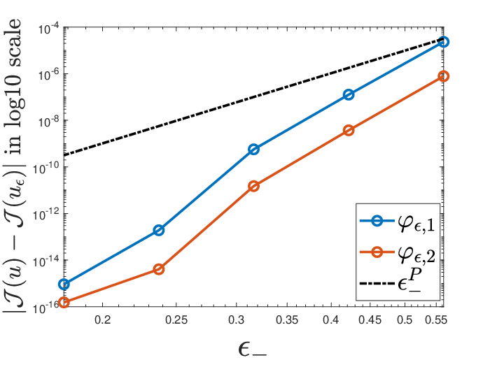
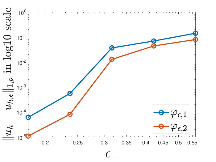
We investigate the effect of regularization parameters $\epsilon$ in this section. In Figure 6, we compare the regularization errors for the regularized models with the following N-functions $\varphi_{\epsilon}$ , where $\varphi_{\epsilon,1}\in C^{1}$ is defined as,

\varphi_{\epsilon,1}(t):=\left\{\begin{array}[]{ll}\frac{1}{2}\epsilon_{-}^{p-2}t^{2}+\left(\frac{1}{p}-\frac{1}{2}\right)\epsilon_{-}^{p}&\text{ for }t\leqslant\epsilon_{-}\\ \frac{1}{p}t^{p}&\text{ for }\epsilon_{-}\leqslant t\leqslant\epsilon_{+}\\ \frac{1}{2}\epsilon_{+}^{p-2}t^{2}+\left(\frac{1}{p}-\frac{1}{2}\right)\epsilon_{+}^{p}&\text{ for }t\geqslant\epsilon_{+}\end{array}\right.

(53)

and a smoother $\varphi_{\epsilon,2}\in C^{2}$ is defined as,

\varphi_{\epsilon,2}(t):=\left\{\begin{array}[]{ll}\frac{1}{p}\epsilon_{-}^{p-2}t^{2}+\frac{p-2}{p^{2}+2p}\epsilon_{-}^{-2}t^{p+2}-\frac{p-2}{p(p+2)}\epsilon_{-}^{p}&\text{ for }t\leqslant\epsilon_{-}\\ \frac{1}{p}t^{p}&\text{ for }\epsilon_{-}\leqslant t\leqslant\epsilon_{+}\\ \frac{p(p-1)}{2}\epsilon_{+}^{p-2}t^{2}+(2-p)\epsilon_{+}^{p-1}t-\frac{p^{2}-3p+2}{2p}\epsilon_{+}^{p}&\text{ for }t\geqslant\epsilon_{+}.\end{array}\right.

(54)

The fine mesh solutions for the original model and regularized models are discretized using piecewise linear finite elements, and solved by Matlab built-in function fminunc (trust region) with first optimality condition below $10^{-7}$ .

From our numerical results in Figure 3 and Figure 6, it seems for $p\geqslant 2$ , the coefficients $\kappa(x)|\nabla u|^{p-2}$ can be degenerate but still bounded from above. Therefore, only the regularization parameter $\epsilon_{-}$ from below is effective in this case. The regularization error has faster decay than $\epsilon_{-}^{p}$ postulated in Assumption 16. We observe that when $\epsilon_{-}^{p-2}\simeq 10^{-6}$ , the error in energy has reached the level of about $10^{-15}$ .

In the following numerical studies, we simply use the regularized model with $\epsilon_{-}^{p-2}=10^{-6}$ which guarantees sufficiently small regularization error as well as the well-posedness of the iterative scheme. For simplicity, we drop the subscript $\epsilon$ from the quantities such as $\mathcal{J}_{\epsilon}$ , $u_{\epsilon}$ , etc.

4.1.2 Comparison of iterative methods

We compare different iterative methods on fine mesh in Figure 7: the implicit quasi-norm based method, the gradient descent method (abbreviated as GD, $w_{GD}^{n}=\Delta^{-1}\mathcal{J}^{\prime}(u^{(n)})$ ), the preconditioned gradient descent (PGD) method and Newton’s method. We consider the regularized $\mathcal{J}_{\epsilon}$ with $\epsilon_{-}^{p-2}=10^{-6}$ . The stopping criterion is $(\mathcal{J}(u^{(n)})-\mathcal{J}(u^{(n+1)}))/|\mathcal{J}(u^{(n)})|\leqslant 10^{-15}$ . We use the Matlab build-in function fminunc for the line search. We choose the initial guess $u^{(0)}$ as the solution of the Poisson’s equation with the coefficient $\kappa(x)$ unless otherwise specified.

As shown in Figure 7, the implicit quasi-norm based method has the best start and exponential convergence in energy as expected by Theorem 11, and Newton’s method achieves best convergence rate as a second order method. PGD has similar convergence rate as the implicit method, which seems to be independent of the heterogeneous coefficient $\kappa(x)$ . The gradient descent method suffers from the heterogeneity of $\kappa(x)$ , and converges very slow. Therefore, an optimal iterative method may combine a starting step with the implicit quasi-norm based method and the consequent iterations with Newton’s method.

4.1.3 Iterated numerical homogenization and residual regularization

We present the implementation details and numerical results for the $L^{2}$ residual regularized iterated numerical homogenization in Section 3.3. Here, we fix the fine mesh size $h=2^{-7}$ , the coarse mesh size $H=2^{-4}$ , and $p=10$ . We implement PGD and Newton’s method on both the coarse mesh and the fine mesh. We take the tolerance $\varepsilon=10^{-15}$ and the threshold $\delta=0.68$ in Algorithm 3.

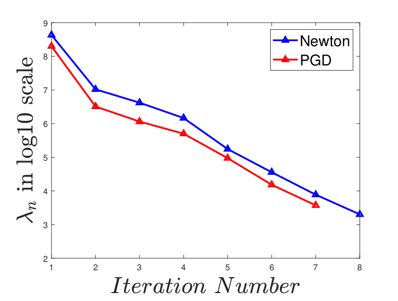
As shown in Figure 8(a), the residual regularized iterated homogenization converges, while the iterated homogenization without residual regularization (green curve in 8(a)) does not converge because of the residual behavior shown in Figure 2. The convergence of the coarse mesh solution is slower than its fine mesh counterpart due to the error of the search direction $w^{(n)}_{H}$ , as well as the residual regularization. For the iterated homogenization with residual regularization, the error of the coarse mesh solution will eventually saturate due to the $O(H^{2})$ homogenization error expected by Theorem 20. In Figures 8(b)(c), the indicator $\rho_{n}$ approaches $0.5$ and the penalty parameter $\lambda_{n}$ decreases during the first 7 or 8 iterations, as a consequence, the residual regularization switches off thereafter. We also plot numerical estimates of $C_{n}$ and $C_{n}^{\prime}$ in Figure 8(d) as a numerical verification of Assumptions 38 and 45. $C_{n}$ is estimated by the solution $\widetilde{C}_{n}$ of the following nonlinear equation,

\widetilde{C}_{n}A[u^{(n)}](w_{0}^{(n)},w_{0}^{(n)})=\int_{\Omega}\kappa(x)\varphi^{\prime\prime}\left(|\nabla u^{(n)}|+\frac{1}{\widetilde{C}_{n}}|\nabla w_{0}^{(n)}|\right)|\nabla w_{0}^{(n)}|^{2}.

where $w_{0}^{(n)}$ is given by $A[u^{(n)}](w_{0}^{(n)},v)=-\mathcal{J}^{\prime}(u^{(n)})(v),\text{ for }\forall v\in\mathcal{V}_{h}$ . $\widetilde{C}^{\prime}_{n}$ is defined similarly. We observe that both $\widetilde{C}_{n}$ and $\widetilde{C}^{\prime}_{n}$ have an upper bound controlled by the contrast of the linearized operators $A[u^{(n)}]$ , and decays to $O(1)$ as $n$ grows.

4.1.4 Homogenization error

We demonstrate the numerical homogenization errors of coarse mesh solutions in Figure 9 and Figure 10, with respect to the coarse degrees of freedom, for PGD and Newton methods, respectively. We show the $H^{1}$ error, the $W^{1,p}$ error, and the energy error of $u_{H}$ with respect to the minimizer $u_{h}\in\mathcal{V}_{h}$ . In this example, we use a fixed fine mesh with $h=2^{-7}$ and varying coarse mesh sizes $H=2^{-2},\,2^{-3},\,2^{-4},\,2^{-5}$ , respectively.

4.2 SPE 10

In this section, we show the performance of the iterated numerical homogenization method for a more challenging example, the SPE10 benchmark problem, which is the set of industry benchmark problems from the Society of Petroleum Engineers (SPE). The coefficients $\kappa(x,y,z)$ are piecewise constant in the domain $[0,220]\times[0,60]\times[0,85]$ . We select $\kappa(x,y,39)$ as the coefficient of the two dimensional problem, with contrast $1.74956\times 10^{7}$ . We rescale the domain to $\Omega=[0,2.2]\times[0,0.6]$ . We take $f=\sin((1/2.2)\pi x)\sin((1/0.6)\pi y)$ , and $p=20$ . In the numerical experiment, we choose $H=1/10$ , $1/20$ , $1/40$ , respectively. The fine mesh size is fixed as $h=1/160$ .

We illustrate the above SPE10 coefficient $\kappa$ , also $|\nabla u|^{p-2}$ and $\kappa|\nabla u|^{p-2}$ in Figure 11(a). We show the reference solution and homogenized solution in Figure 11(b), which visually match with each other.

We further show the homogenization error in Figure 12. Although the energy error has similar decay, but the $H^{1}$ and $W^{1,p}$ errors are not as good as the mstrig example in Section 4.1.

4.3 Sparse Updating

In the iterated homogenization method, we need to update the coarse space $\mathcal{V}_{H}^{(n)}$ in every iteration, which may contribute to a significant part of the computational cost. However, apart from the first several steps of the iteration, as $u^{(n)}$ converges to the true solution $u$ , the linearized operator $A[u^{(n)}]$ also converges to $A[u]$ . Therefore, we propose a sparse updating scheme for the efficient construction of the coarse space $\mathcal{V}_{H}^{(n)}$ in the iterated numerical homogenization.

Here we propose a simple indicator to switch on/off basis update, and we refer to [45] for more rigorous analysis. We recall that a single basis of $\mathcal{V}_{H}^{(n)}$ only depends locally on the coefficient of $A[u^{(n)}]$ through $\kappa(x)$ and $|\nabla u^{(n)}|$ . Denote by $\phi_{i}^{(n,n+1)}(\tau)$ the corresponding basis of the operator $A[u^{(n)}+\tau(u^{(n+1)}-u^{(n)})]$ , and by $\mathbf{B}^{(n,n+1)}(\tau)$ their stiffness matrix. The components of $\mathbf{B}^{(n,n+1)}(\tau)$ write $\mathbf{B}_{i,j}^{(n,n+1)}(\tau)=A[u^{(n)}+\tau(u^{(n+1)}-u^{(n)})](\phi_{i}^{(n,n+1)}(\tau),\phi_{j}^{(n,n+1)}(\tau))$ . Let

\mathcal{I}_{i}^{(n)}:=\frac{d\mathbf{B}_{i,i}^{(n,n+1)}(\tau)}{d\tau}\Big|_{\tau=0}=A[(u^{(n+1)}-u^{(n)})](\phi_{i}^{n},\phi_{i}^{n}),

we may take $\mathcal{I}_{i}^{(n)}$ as an indicator for basis updating. Using indicator $\mathcal{I}_{i}^{(n)}$ for $n\geqslant 1$ , we can reformulate the STEP 2 of Algorithms 2 and 3 as below,

STEP 2:

n=0

then

Construct a coarse space

\mathcal{V}^{(0)}_{H}:={\rm span}\{\phi^{(0)}_{i},i=1,...,N_{H}\}

, and each

\phi^{(0)}_{i}

is obtained by solving a constrained minimization problem (3) associated with the quadratic form

A[u^{(0)}]

else

for

i=1..N_{H}

Calculate

\mathcal{I}_{i}^{(n)}

\mathcal{I}_{i}^{(n)}\geqslant\delta_{\mathcal{I}}

then

Calculate new basis

\phi_{i}^{(n)}

by solving (3) associated with the quadratic form

A[u^{(n)}]

else

\phi_{i}^{(n)}:=\phi_{i}^{(n-1)}

end if

end for

\mathcal{V}^{(n)}_{H}:={\rm span}\{\phi^{(n)}_{i},i=1,...,N_{H}\}

end if

Table 1: Efficiency Improvement for

p=15

\kappa(x)=spe10

	Efficiency	Accuracy( $H^{1}$ )
Full Updating	100%	0.67e-2
$\delta_{\mathcal{I}}=4e-8$	80.94%	0.73e-2
$\delta_{\mathcal{I}}=2e-8$	80.23%	0.79e-2
$\delta_{\mathcal{I}}=1e-8$	68.68%	1.08e-2

Table 2: Efficiency Improvement for

p=20

\kappa(x)=spe10

	Efficiency	Accuracy( $H^{1}$ )
Full Updating	100%	0.44e-2
$\delta_{\mathcal{I}}=4e-9$	84.89%	0.48e-2
$\delta_{\mathcal{I}}=6e-9$	65.42%	0.75e-2
$\delta_{\mathcal{I}}=1e-8$	55.75%	0.82e-2

In Table 2 and Table 2, we show the total number of basis updating (Efficiency) versus the parameter $\delta_{\mathcal{I}}$ , for spe10 example with $p=15,20$ , respectively. It seems the sparse updating is more effective for more nonlinear problem ( $p=20$ ).

5 Conclusion

In this paper we propose the iterated numerical homogenization method for multi-scale elliptic equations with monotone nonlinearity. We combine the iterative methods inspired by the quasi-norm based approach and the numerical homogenization for each linearized operator in the nonlinear iteration. The residual regularized line search is proposed to ensure the convergence of the iterated numerical homogenization up to coarse resolution. We offer a number of representative numerical examples to illustrate and validate the proposed method.

We plan to study more complicated nonlinear multiscale problems, for example, problems with nonconvex flux, and nonlinear heterogeneous elasticity. We also plan to study the use of nonlocal upscaling techniques [21, 19].

6 Acknowledgements

X.L and L.Z are partially supported by the National Natural Science Foundation of China (NSFC 11871339, 11861131004). E.C. is partially supported by the Hong Kong RGC General Research Fund (Project numbers 14304719 and 14302018).

References

[1] Assyr Abdulle and Gilles Vilmart. Analysis of the finite element heterogeneous multiscale method for quasilinear elliptic homogenization problems. Mathematics of Computation, 83(286):513–536, 2014.
[2] G. Allaire and R. Brizzi. A multiscale finite element method for numerical homogenization. SIAM J. Multiscale Modeling and Simulation, 4(3):790–812, 2005.
[3] Grégoire Allaire. Homogenization and two-scale convergence. SIAM Journal on Mathematical Analysis, 23(6):1482–1518, 1992.
[4] T. Arbogast. Analysis of a two-scale, locally conservative subgrid upscaling for elliptic problems. SIAM J. Numer. Anal., 42(2):576–598 (electronic), 2004.
[5] J. W. Barrett and W. B. Liu. Finite-element approximation of the p-laplacian. Mathematics of Computation, 61(204):523–537, 1993.
[6] Y Bazilevs, VM Calo, JA Cottrell, TJR Hughes, A Reali, and G Scovazzi. Variational multiscale residual-based turbulence modeling for large eddy simulation of incompressible flows. Computer Methods in Applied Mechanics and Engineering, 197(1):173–201, 2007.
[7] Leonid Berlyand, Alexander G Kolpakov, and Alexei Novikov. Introduction to the network approximation method for materials modeling, volume 148. Cambridge University Press, 2013.
[8] Leonid Berlyand and Houman Owhadi. Flux norm approach to finite dimensional homogenization approximations with non-separated scales and high contrast. Archive for rational mechanics and analysis, 198(2):677–721, 2010.
[9] L. M. Bregman. The relaxation method of finding the common points of convex sets and its application to the solution of problems in convex programming. USSR Computational Mathematics and Mathematical Physics, 7(3):200–217, 1967.
[10] Max Budninskiy, Houman Owhadi, and Mathieu Desbrun. Operator-adapted wavelets for finite-element differential forms. Journal of Computational Physics, 388:144–177, 2019.
[11] Eduardo Casas, Peter I Kogut, and Günter Leugering. Approximation of optimal control problems in the coefficient for the p-laplace equation. i. convergence result. SIAM Journal on Control and Optimization, 54(3):1406–1422, 2016.
[12] P Ponte Castañeda, Józef Joachim Telega, and Barbara Gambin. Nonlinear Homogenization and Its Applications to Composites, Polycrystals and Smart Materials: Proceedings of the NATO Advanced Research Workshop, Held in Warsaw, Poland, 23-26 June 2003, volume 170. Springer Science & Business Media, 2006.
[13] Jiong Chen, Hujun Bao, Tianyu Wang, Mathieu Desbrun, and Jin Huang. Numerical coarsening using discontinuous shape functions. ACM Trans. Graph., 37(4):Art. 117, 2018.
[14] Jiong Chen, Max Budninskiy, Houman Owhadi, Hujun Bao, Jin Huang, and Mathieu Desbrun. Material-adapted refinable basis functions for elasticity simulation. ACM Trans. Graph. (SIGGRAPH Asia), 38(6):Art. 161, 2019.
[15] Valeria ChiadòPiat and Anneliese Defranceschi. Homogenization of monotone operators. Nonlinear Analysis: Theory, Methods & Applications, 14(9):717–732, 1990.
[16] Bruno Christ, Uta Dahmen, Karl-Heinz Herrmann, Matthias König, Jürgen R. Reichenbach, Tim Ricken, Jana Schleicher, Lars Ole Schwen, Sebastian Vlaic, and Navina Waschinsky. Computational modeling in liver surgery. Front Physiol., 8:906, 2017.
[17] Eric Chung, Bernardo Cockburn, and Guosheng Fu. The staggered dg method is the limit of a hybridizable dg method. SIAM Journal on Numerical Analysis, 52(2):915–932, 2014.
[18] Eric Chung, Yalchin Efendiev, Ke Shi, and Shuai Ye. A multiscale model reduction method for nonlinear monotone elliptic equations in heterogeneous media. Networks & Heterogeneous Media, 12(4):619, 2017.
[19] Eric T Chung, Yalchin Efendiev, Wing T Leung, and Mary Wheeler. Nonlinear nonlocal multicontinua upscaling framework and its applications. International Journal for Multiscale Computational Engineering, 16(5), 2018.
[20] Eric T Chung, Yalchin Efendiev, and Wing Tat Leung. An adaptive generalized multiscale discontinuous galerkin method (GMsDGM) for high-contrast flow problems. arXiv preprint arXiv:1409.3474, 2014.
[21] Eric T Chung, Yalchin Efendiev, Wing Tat Leung, Maria Vasilyeva, and Yating Wang. Non-local multi-continua upscaling for flows in heterogeneous fractured media. Journal of Computational Physics, 372:22–34, 2018.
[22] ET Chung, Y Efendiev, and WT Leung. Residual-driven online generalized multiscale finite element methods. To appear in J. Comput. Phys., 2015.
[23] ET Chung, Y Efendiev, and G Li. An adaptive GMsFEM for high-contrast flow problems. Journal of Computational Physics, 273:54–76, 2014.
[24] Bernardo Cockburn, Jayadeep Gopalakrishnan, and Raytcho Lazarov. Unified hybridization of discontinuous galerkin, mixed, and continuous galerkin methods for second order elliptic problems. SIAM Journal on Numerical Analysis, 47(2):1319–1365, 2009.
[25] L. Diening, M. Fornasier, R. Tomasi, and M. Wank. A relaxed kačanov iteration for the p-poisson problem. Numerische Mathematik, 145:1–34, 2020.
[26] L. Diening and Ch. Kreuzer. Linear convergence of an adaptive finite element method for the p-laplacian equation. SIAM J. Numer. Anal., 46(2):614–638, 2008.
[27] L. Diening, Ch. Kreuzer, and E. Süli. Finite element approximation of steady flows of incompressible fluids with implicit power-law-like rheology. SIAM Journal on Numerical Analysis, 51(2):984–1015, 2013.
[28] L. Diening and M. Růžiička. Interpolation operators in orlicz–sobolev spaces. Numerische Mathematik, 107:107–129, 2007.
[29] Lars Diening and Frank Ettwein. Fractional estimates for non-differentiable elliptic systems with general growth. Forum Mathematicum, 20(3):523 – 556, 01 May. 2008.
[30] L.J. Durlofsky. Numerical calculation of equivalent grid block permeability tensors for heterogeneous porous media. Water Resour. Res., 27:699–708, 1991.
[31] W. E and B. Engquist. Heterogeneous multiscale methods. Comm. Math. Sci., 1(1):87–132, 2003.
[32] Carsten Ebmeyer and WB Liu. Quasi-norm interpolation error estimates for the piecewise linear finite element approximation of p-laplacian problems. Numerische Mathematik, 100(2):233–258, 2005.
[33] Y. Efendiev and J. Galvis. Coarse-grid multiscale model reduction techniques for flows in heterogeneous media and applications. Chapter of Numerical Analysis of Multiscale Problems, Lecture Notes in Computational Science and Engineering, Vol. 83, pages 97–125, 2012.
[34] Y. Efendiev, J. Galvis, and T. Hou. Generalized multiscale finite element methods. Journal of Computational Physics, 251:116–135, 2013.
[35] Y. Efendiev, J. Galvis, S. Ki Kang, and R.D. Lazarov. Robust multiscale iterative solvers for nonlinear flows in highly heterogeneous media. Numer. Math. Theory Methods Appl., 5(3):359–383, 2012.
[36] Y. Efendiev, J. Galvis, and X.H. Wu. Multiscale finite element methods for high-contrast problems using local spectral basis functions. Journal of Computational Physics, 230:937–955, 2011.
[37] Y. Efendiev and T. Hou. Multiscale Finite Element Methods: Theory and Applications. Springer, 2009.
[38] Y. Efendiev, T. Hou, and V. Ginting. Multiscale finite element methods for nonlinear problems and their applications. Comm. Math. Sci., 2:553–589, 2004.
[39] Y. Efendiev and A. Pankov. Numerical homogenization and correctors for nonlinear elliptic equations. SIAM J. Appl. Math., 65(1):43–68, 2004.
[40] Yalchin Efendiev, J Galvis, M Presho, and J Zhou. A multiscale enrichment procedure for nonlinear monotone operators. ESAIM: Mathematical Modelling and Numerical Analysis, 48(02):475–491, 2014.
[41] Yalchin Efendiev, Raytcho Lazarov, Minam Moon, and Ke Shi. A spectral multiscale hybridizable discontinuous Galerkin method for second order elliptic problems. Computer Methods in Applied Mechanics and Engineering, 292:243–256, 2015.
[42] Abderrahim Elmoataz, Matthieu Toutain, and Daniel Tenbrinck. On the p-laplacian and $\infty$ -laplacian on graphs with applications in image and data processing. SIAM Journal on Imaging Sciences, 8(4):2412–2451, 2015.
[43] Frédéric Feyel. Multiscale fe2 elastoviscoplastic analysis of composite structures. Computational Materials Science, 16(1-4):344–354, 1999.
[44] Marc GD Geers, Varvara G Kouznetsova, Karel Matouš, and Julien Yvonnet. Homogenization methods and multiscale modeling: nonlinear problems. Encyclopedia of Computational Mechanics Second Edition, pages 1–34, 2017.
[45] Fredrik Hellman and Axel Målqvist. Numerical homogenization of elliptic pdes with similar coefficients. Multiscale Modeling & Simulation, 17(2):650–674, 2019.
[46] Patrick Henning. Heterogeneous multiscale finite element methods for advection-diffusion and nonlinear elliptic multiscale problems. Münster: Univ. Münster, Mathematisch-Naturwissenschaftliche Fakultät, Fachbereich Mathematik und Informatik (Diss.). ii, page 63, 2011.
[47] Patrick Henning and Mario Ohlberger. Error control and adaptivity for heterogeneous multiscale approximations of nonlinear monotone problems. Discrete and Continuous Dynamical Systems-Serie S. Special Issue on Numerical Methods based on Homogenization and Two-Scale Convergence, 2015.
[48] Yunqing Huang, Ruo Li, and Wenbin Liu. Preconditioned descent algorithms for p-laplacian. Journal of Scientific Computing, 32(2):343–371, 2007.
[49] T. J. R Hughes, G. Feijoo, L. Mazzei, and J. Quincy. The variational multiscale method—a paradigm for computational mechanics. Comput. Methods Appl. Mech. Engrg., 166:3–24, 1998.
[50] V.V. Jikov, S. M. Kozlov, and O. A. Oleinik. Homogenization of differential operators and integral functionals. Springer Science & Business Media, 2012.
[51] Lily Kharevych, Patrick Mullen, Houman Owhadi, and Mathieu Desbrun. Numerical coarsening of inhomogeneous elastic materials. ACM Transactions on Graphics (SIGGRAPH), 28(3), 2009.
[52] Mark Aleksandrovich Krasnoselskiiĭ. Convex functions and Orlicz spaces, volume 4311. US Atomic Energy Commission, 1960.
[53] J. Leray and J. L. Lions. Quelques résulatats de višik sur les problèmes elliptiques nonlinéaires par les méthodes de minty-browder. Bull. Soc. Math. France, 93:97–107, 1965.
[54] J. L. Lions, D. Lukkassen, L. E. Persson, and P. Wall. Reiterated homogenization of nonlinear monotone operators. Chinese Annals of Mathematics, 22(01):1–12, 2001.
[55] W. B. Liu and J. W. Barrett. A remark on the regularity of the solutions of the p-laplacian and its application to their finite-element approximation. Journal of Mathematical Analysis and Applications, 178(2):470–487, 1993.
[56] X. Liu, L. Zhang, and Zhu S. Generalized polyharmonic splines for multiscale pdes with rough coefficients. Preprint, 2018.
[57] Pingbing Ming, Pingwen Zhang, et al. Analysis of the heterogeneous multiscale method for elliptic homogenization problems. Journal of the American Mathematical Society, 18(1):121–156, 2005.
[58] Gabriel Nguetseng and Hubert Nnang. Homogenization of nonlinear monotone operators beyond the periodic setting. Electr. J. of Diff. Eqns, 36:1–24, 2003.
[59] Jorge Nocedal and Stephen Wright. Numerical optimization. Springer Science & Business Media, 2006.
[60] H. Owhadi. Multigrid with rough coefficients and Multiresolution operator decomposition from Hierarchical Information Games. SIAM Rev., 59(1):99–149, March 2017.
[61] H. Owhadi and L. Zhang. Localized bases for finite dimensional homogenization approximations with non-separated scales and high-contrast. SIAM Multiscale Model. Simul., 9(4):1373–1398, 2011.
[62] H. Owhadi, L. Zhang, and L. Berlyand. Polyharmonic homogenization, rough polyharmonic splines and sparse super-localization. ESAIM: Math. Model. Numer. Anal., 48(2):517–552, 2014.
[63] Houman Owhadi, Lei Zhang, and Leonid Berlyand. Polyharmonic homogenization, rough polyharmonic splines and sparse super-localization. ESAIM: Mathematical Modelling and Numerical Analysis, 48(02):517–552, 2014.
[64] Aleksandr Andreevich Pankov. G-convergence and homogenization of nonlinear partial differential operators, volume 422. Springer Science & Business Media, 2013.
[65] G Papanicolau, A Bensoussan, and J-L Lions. Asymptotic analysis for periodic structures. Elsevier, 1978.
[66] Mohammad Mamunur Rahman, Yusheng Feng, Thomas E. Yankeelov, and J. Tinsley Odenb. A fully coupled space–time multiscale modeling framework for predicting tumor growth. Comput Methods Appl Mech Eng., 320:261–286, 2017.
[67] Malempati Madhusudana Rao and Zhong Dao Ren. Applications of Orlicz spaces, volume 250. CRC Press, 2002.
[68] Dejan Slepčev and Matthew Thorpe. Analysis of $p$ -laplacian regularization in semi-supervised learning. arXiv preprint arXiv:1707.06213, 2017.
[69] X.H. Wu, Y. Efendiev, and T.Y. Hou. Analysis of upscaling absolute permeability. Discrete and Continuous Dynamical Systems, Series B., 2:158–204, 2002.

Appendix A Appendix

A.1 Property of N-functions

For a given N-function $\varphi$ , we define the N-function $\psi$ by $\frac{\psi^{\prime}(t)}{t}:=(\frac{\varphi^{\prime}(t)}{t})^{\frac{1}{2}}$ , and $\mathbf{V}(\bm{\xi}):=(\nabla\bm{\Psi})(\bm{\xi})=\psi^{\prime}(|\bm{\xi}|)\frac{\xi}{|\bm{\xi}|}$ . We collect the following results from [28, 29].

Lemma 21.

Let $a(x,\bm{\xi})=\kappa(x)\varphi^{\prime}(|\bm{\xi}|)\frac{\bm{\xi}}{|\bm{\xi}|}$ , we have

$\displaystyle(a(x,\bm{\xi})-a(x,\bm{\zeta}))\cdot(\bm{\xi}-\bm{\zeta})$	$\displaystyle\sim\varphi_{\|\bm{\xi}\|}(\|\bm{\xi}-\bm{\zeta}\|)$	(55)
	$\displaystyle\sim\|\mathbf{V}(\bm{\xi})-\mathbf{V}(\bm{\zeta})\|^{2}$
	$\displaystyle\sim\varphi^{\prime\prime}(\|\bm{\xi}\|+\|\bm{\zeta}\|)\|\bm{\xi}-\bm{\zeta}\|^{2}.$

Lemma 22 (Young type inequality).

Let $\varphi$ be an N-function with $\Delta_{2}({\varphi,\varphi^{*}})<\infty$ . For all $\delta>0$ , we have the following Young’s inequality, where $C_{\delta}$ only depends on $\Delta_{2}({\varphi,\varphi^{*}})$ , such that for all $t$ , $s$ , $a\geqslant 0$ ,

t\varphi^{\prime}_{a}(s)+s\varphi^{\prime}_{a}(t)\leqslant\delta\varphi_{a}(t)+c_{\delta}\varphi_{a}(s).

(56)

Lemma 23.

Let the N-function $\varphi$ satisfy Assumption 1, then uniformly in $s$ , $t\in\mathbb{R}$ , we have

	$\displaystyle\varphi^{\prime\prime}(\|s\|+\|t\|)\|s-t\|$	$\displaystyle\sim\varphi^{\prime}_{\|s\|}(\|s-t\|),$		(57)
	$\displaystyle\varphi^{\prime\prime}(\|s\|+\|t\|)\|s-t\|^{2}$	$\displaystyle\sim\varphi_{\|s\|}(\|s-t\|).$		(57)

Lemma 24.

Let the N-function $\varphi$ satisfy Assumption 1, then uniformly in $s$ , $t\in\mathbb{R}$ , we have

\varphi_{|s|}(|s-t|)\sim\varphi_{|t|}(|s-t|).

(58)

The following inequality is the consequence of the Young type inequality, Property 3, and Lemma 57,

$\displaystyle(a(x,\nabla u)-a(x,\nabla v))(\nabla w-\nabla v)$	$\displaystyle\leqslant\|(a(x,\nabla u)-a(x,\nabla v))\|\cdot\|(\nabla w-\nabla v)\|$	(59)
	$\displaystyle\leqslant c\varphi^{\prime\prime}(\|\nabla u\|+\nabla v\|)\|\nabla u-\nabla v\|\cdot\|\nabla w-\nabla v\|$
	$\displaystyle\leqslant c\varphi^{\prime}_{\|\nabla u\|}(\|\nabla u-\nabla v\|)\|\nabla w-\nabla v\|$
	$\displaystyle\leqslant\delta\varphi_{\|\nabla u\|}(\|\nabla u-\nabla v\|)+c_{\delta}\varphi_{\|\nabla u\|}(\|\nabla w-\nabla v\|).$

A.2 Orlicz Space

We give some characterizations of the Orlicz space and Sobolev Orlicz space according to [52, 67].

Theorem 25.

Let $\varphi$ be an N-function with $\Delta_{2}(\varphi,\varphi^{*})<\infty$ , the following statements are true:

(1)

$L^{\varphi}(\Omega)$ is normed with $\|w\|_{L^{\varphi}(\Omega)}:=\inf\left\{\lambda>0:\int_{\Omega}\varphi\left(\frac{|w|}{\lambda}\right)dx\leqslant 1\right\}$ . We note that this norm coincides with $L^{p}$ norm for $\varphi=t^{p}/p$ .
(2)

A sequence of functions $\left\{w_{n}\right\}$ in $L^{\varphi}(\Omega)$ converges to $w\in L^{\varphi}(\Omega)$ with respect to $\|\cdot\|_{L^{\varphi}(\Omega)}$ , if and only if $\int_{\Omega}\varphi\left(\left|w_{n}-w\right|\right)dx\stackrel{{\scriptstyle n\rightarrow\infty}}{{\longrightarrow}}0,$
(3)

$L^{\varphi}(\Omega)$ is complete, separable and reflexive.

Definition 26.

For an N-function $\varphi$ satisfying the $\Delta_{2}$ condition we define the Orlicz Sobolev space via

W^{1,\varphi}(\Omega):=\left\{w\in L^{\varphi}(\Omega):\forall i\in\{1,\ldots,d\},\frac{\partial}{\partial x_{i}}w\in L^{\varphi}(\Omega)\right\}.

where $\frac{\partial}{\partial x_{i}}w$ denotes the weak derivative in the $i$ -th direction.

Definition 27.

For an N-function $\varphi$ , we define its Simonenko indices via

p^{-}:=\inf_{t>0}\frac{t\varphi^{\prime}(t)}{\varphi(t)}<\sup_{t>0}\frac{t\varphi^{\prime}(t)}{\varphi(t)}=:p^{+}.

If $p^{+}<\infty$ , $\varphi$ satisfies the $\Delta_{2}$ condition.

Theorem 28.

Let $\varphi$ be an N-function with $p^{-},p^{+}\in(1,\infty).$ Then, the following statements are true:

(1)

$W^{1,\varphi}(\Omega)$ is normed with $\|w\|_{W^{1,\varphi(\Omega)}}:=\|w\|_{L^{\varphi}(\Omega)}+\sum_{i=1}^{d}\left\|\frac{\partial}{\partial x_{i}}w\right\|_{L^{\varphi}(\Omega)}$ .
(2)

A sequence of functions $\left\{w_{n}\right\}$ in $W^{1,\varphi}(\Omega)$ converges to $w\in W^{1,\varphi}(\Omega)$ with respect to $\|\cdot\|_{W^{1,\varphi(\Omega)}}$ , if and only if $\int_{\Omega}\varphi\left(\left|w_{n}-w\right|\right)dx\stackrel{{\scriptstyle n\rightarrow\infty}}{{\longrightarrow}}0$ , and for all $i\in\{1,\ldots,d\}$ also $\int_{\Omega}\varphi\left(\left|\frac{\partial}{\partial x_{i}}\left(w_{n}-w\right)\right|\right)dx\stackrel{{\scriptstyle n\rightarrow\infty}}{{\longrightarrow}}0$ .
(3)

$W^{1,\varphi}(\Omega)$ is complete, separable and reflexive.

Definition 29.

We define the homogeneous Orlicz Sobolev space as $W_{0}^{1,\varphi}(\Omega):=\overline{C_{0}^{\infty}(\Omega)}^{\|\cdot\|_{W^{1,\varphi}(\Omega)}}$ . Note that Poincaré’s Inequality also holds for the homogeneous Orlicz Sobolev space.

Proposition 30.

Under Assumption 1, $\varphi^{\prime\prime}(t)$ is a non-decreasing function, which implies that the Simonenko index of $\varphi$ , $p^{-}\geqslant 2$ . Furthermore, $\mathcal{J}$ is differentiable and second order Gateaux differentiable. Its derivative and second order derivative are given in (5) and (6), and well-defined.

A.3 Proof of Lemma 4

Lemma 31.

For any $u$ , $v$ , and $s\in[0,1]$ , we have

s/2(|\nabla v|+|\nabla(u-v)|)\leqslant|\nabla(v+s(u-v))|+|\nabla v|\leqslant 2(|\nabla v|+|\nabla(u-v)|).

(60)

In particular, for $s=1$ , we have

1/2(|\nabla v|+|\nabla(u-v)|)\leqslant|\nabla v|+|\nabla u|\leqslant 2(|\nabla v|+|\nabla(u-v)|).

(61)

Proof.

Assumption 1 implies that $\varphi(t)\sim t\varphi^{\prime}(t)\sim t^{2}\varphi^{\prime\prime}(t)$ , and by the $\Delta_{2}(\varphi)$ condition, we also have $\varphi(2t)\leqslant c\varphi(t)$ . Therefore, it holds true that $4t^{2}\varphi^{\prime\prime}(2t)\leqslant ct^{2}\varphi^{\prime\prime}(t)$ uniformly for $t\geqslant 0$ . Denoting $w=u-v$ , we have

\begin{aligned} \mathcal{D}_{\mathcal{J}}(u,v)&=\mathcal{J}(u)-\mathcal{J}(v)-\mathcal{J}^{\prime}(v)(u-v)\\ &=\int_{0}^{1}\mathcal{J}^{\prime}(v+sw)w-\mathcal{J}^{\prime}(v)w\mathrm{ds}\\ &=\int_{0}^{1}\frac{1}{s}(\mathcal{J}^{\prime}(v+sw)-\mathcal{J}^{\prime}(v))(sw)\mathrm{ds}\\ &\geqslant c\int_{0}^{1}s\int\kappa(x)\varphi^{\prime\prime}(|\nabla v+s\nabla w|+|\nabla v|)|\nabla w|^{2}\mathrm{dx}\mathrm{ds}\\ &\geqslant c\int\kappa(x)\varphi^{\prime\prime}(|\nabla v|+|\nabla w|)|\nabla u-\nabla v|^{2}\mathrm{dx},\end{aligned}.

(62)

and

\begin{aligned} \mathcal{D}_{\mathcal{J}}(u,v)&=\mathcal{J}(u)-\mathcal{J}(v)-\mathcal{J}^{\prime}(v)(u-v)\\ &=\int_{0}^{1}\mathcal{J}^{\prime}(v+sw)w-\mathcal{J}^{\prime}(v)w\mathrm{ds}\\ &\leqslant\int_{0}^{1}\int\kappa(x)\varphi^{\prime\prime}(|\nabla v+s\nabla w|+|\nabla v|)s|\nabla w|^{2}\mathrm{ds}\\ &\leqslant C\int\kappa(x)\varphi^{\prime\prime}(|\nabla v|+|\nabla w|)|\nabla u-\nabla v|^{2}\mathrm{dx}.\end{aligned}.

(63)

A.4 Proof of Lemma 15

Proof.

It is clear that we regularize when $|\nabla u|$ vanishes or becomes large.

For $u\in W_{0}^{1,p}(\Omega)$ , we define $\Omega_{k}(u):=\left\{x\in\Omega:|\nabla u(x)|>k\right\}$ . By following inequalities

\left|\Omega_{k}(u)\right|:=\int_{\Omega_{k}(u)}1\leqslant\frac{1}{k}\int_{\Omega_{k}(u)}|\nabla u|\leqslant\frac{1}{k}\left|\Omega_{k}(u)\right|^{\frac{1}{q}}\left(\int_{\Omega}|\nabla u|^{p}d\right)^{\frac{1}{p}}=\frac{\|u\|_{W_{0}^{1,p}(\Omega)}}{k}\left|\Omega_{k}(u)\right|^{\frac{p-1}{p}},

we have $\left|\Omega_{k}(u)\right|\leq\|u\|_{W_{0}^{1,p}(\Omega)}^{p}k^{-p}$ , for all $u\in W_{0}^{1,p}(\Omega)$ . Similarly, we have

\left|\Omega_{k}(u)\right|\leqslant\frac{1}{k^{p}}\left(\int_{\Omega_{k}(u)}a_{\epsilon}(x,\nabla u)\cdot\nabla u\right),\quad\forall u\in W_{0}^{1,2}(\Omega),

(64)

where $a_{\epsilon}(x,\nabla u)=\varphi_{\epsilon_{k}}^{\prime}(|\nabla u|)\nabla u/|\nabla u|$ . Therefore, $\left|\Omega_{k}(u)\right|\rightarrow 0$ , as $\epsilon_{+,k}\rightarrow\infty$ .

Step 1: The sequence $u_{\epsilon_{k}}$ is bounded in $H^{1}_{0}$ .

Taking $v=u_{\epsilon_{k}}$ in

\int_{\Omega}a_{\epsilon_{k}}(x,\nabla u_{\epsilon_{k}})\cdot\nabla v=(f,v),\quad\forall v\in H_{0}^{1},

(65)

and combining the fact that

	$\displaystyle\\|\nabla u_{\epsilon_{k}}\\|_{L^{2}\left(\Omega\backslash\Omega_{k}(u_{\epsilon_{k}})\right)^{d}}$	$\displaystyle\leq\|\Omega\|^{\frac{p-2}{2p}}\\|\nabla u_{\epsilon_{k}}\\|_{L^{p}\left(\Omega\backslash\Omega_{k}(u_{\epsilon_{k}})\right)^{d}}$		(66)
		$\displaystyle\leqslant\|\Omega\|^{\frac{p-2}{2p}}\left(\int_{\Omega\backslash\Omega_{k}(u)}a_{\epsilon}(x,\nabla u_{\epsilon_{k}})\cdot\nabla u_{\epsilon_{k}}\right)^{\frac{1}{p}},$		(66)

and

\|\nabla u_{\epsilon_{k}}\|_{L^{2}\left(\Omega_{k}(u_{\epsilon_{k}})\right)^{N}}\leqslant|\Omega|^{\frac{p-2}{2p}}\left(\int_{\Omega_{k}(u_{\epsilon_{k}})}a_{\epsilon}(x,\nabla u_{\epsilon_{k}})\cdot\nabla u_{\epsilon_{k}}\right)^{\frac{1}{2}},

(67)

we have

	$\displaystyle\int_{\Omega}a_{\epsilon_{k}}(x,\nabla u_{\epsilon_{k}})\cdot\nabla u_{\epsilon_{k}}$	$\displaystyle=(f,u_{\epsilon_{k}})\leqslant\\|f\\|_{L^{2}}\\|\nabla u_{\epsilon_{k}}\\|_{L^{2}}$		(68)
		$\displaystyle\leqslant C\\|f\\|_{L^{2}}\left(\int_{\Omega}a_{\epsilon_{k}}(x,\nabla u_{\epsilon_{k}})\cdot\nabla u_{\epsilon_{k}}\right)^{1/2}.$		(68)

Therefore, $\int_{\Omega}a_{\epsilon_{k}}(x,\nabla u_{\epsilon_{k}})\cdot\nabla u_{\epsilon_{k}}$ (hence $\|u_{\epsilon_{k}}\|_{H_{0}^{1}}$ ) is also uniformly bounded.

Step 2 : (Lemma 5.1 in Casas [11]) weak limit $u$ of $u_{\epsilon_{k}}$ belongs to $W^{1,p}$ .

Since $\{u_{\epsilon_{k}}\}$ is uniformly bounded in $H^{1}_{0}$ , we can extract a subsequence which converge weakly to $u\in H^{1}_{0}$ . Without loss of generality, we assume the subsequence is $\{u_{\epsilon_{k}}\}$ itself.

We fix an index $k\in\mathrm{N}$ and associate it with the set: $B_{k}:=\bigcup_{j=k}^{\infty}\Omega_{j}\left(u_{\epsilon_{j}}\right)$ , where $\Omega_{j}\left(u_{\epsilon_{j}}\right):=\left\{x\in\Omega:\left|\nabla u_{\epsilon_{j}}(x)\right|>j\right\}$ .

By the estimate (64) and uniformly boundedness of $\int_{\Omega}a_{\epsilon_{k}}(x,\nabla u_{\epsilon_{k}})\cdot\nabla u_{\epsilon_{k}}$ , we see that

\left|B_{k}\right|\leqslant C\sum_{j=k}^{\infty}\frac{1}{j^{p}}<+\infty,

and, therefore $\lim_{k\rightarrow\infty}\left|B_{k}\right|=0$ . We also have

\displaystyle\int_{\Omega\backslash B_{k}}\kappa(x)\left|\nabla u_{\epsilon_{j}}\right|^{p}dx

\displaystyle\leqslant\int_{\Omega}a_{\epsilon_{j}}(x,\nabla u_{\epsilon_{j}})\cdot\nabla u_{\epsilon_{j}}\leqslant C,\,\forall j\geqslant k,

hence $\left\{\nabla u_{\epsilon_{j}}\right\}$ is bounded in $L^{p}\left(\Omega\backslash B_{k}\right)^{N}$ . Since $\nabla u_{\epsilon_{j}}\rightharpoonup\nabla u$ in $L^{2}(\Omega)^{d}$ , we have $\nabla u_{\epsilon_{j}}\rightharpoonup\nabla u$ in $L^{p}(\Omega\backslash{B_{k}})^{d}$ . Hence,

	$\displaystyle\int_{\Omega}\frac{1}{p}\kappa(x)\|\nabla u\|^{p}$	$\displaystyle=\lim_{k\rightarrow\infty}\int_{\Omega\backslash B_{k}}\frac{1}{p}\kappa(x)\|\nabla u\|^{p}\leqslant\lim_{k\rightarrow\infty}\liminf_{\begin{subarray}{c}j\rightarrow\infty\\ j\geqslant k\end{subarray}}\int_{\Omega\backslash B_{k}}\frac{1}{p}\kappa(x)\left\|\nabla u_{\epsilon_{j}}\right\|^{p}$		(69)
		$\displaystyle\leqslant\liminf_{j\rightarrow\infty}\int_{\Omega\backslash\Omega_{j}}\kappa(x)\varphi_{\epsilon_{j}}(\|\nabla u_{\epsilon_{j}}\|)\leqslant\liminf_{j\rightarrow\infty}\int_{\Omega}\kappa(x)\varphi_{\epsilon_{j}}(\|\nabla u_{\epsilon_{j}}\|).$		(69)

Moreover,

\mathcal{J}(u)=\int_{\Omega}\frac{1}{p}\kappa(x)|\nabla u|^{p}-fu\leqslant\liminf_{j\rightarrow\infty}\int_{\Omega}\kappa(x)\varphi_{\epsilon_{j}}(|\nabla u_{\epsilon_{j}}|)-fu_{\epsilon_{j}}=\liminf_{j\rightarrow\infty}\mathcal{J}_{\epsilon}(u_{\epsilon_{j}}).

(70)

Let $u^{*}$ be the minimizer of $\mathcal{J}$ in $W^{1,p}$ , we have

\mathcal{J}(u^{*})\leqslant\mathcal{J}(u)\leqslant\liminf_{j\rightarrow\infty}\mathcal{J}_{\epsilon}(u_{\epsilon_{j}}).

(71)

Using the definition (53) or (54) of $\varphi_{\epsilon}$ , for any $u\in W_{0}^{1,p}$ , we have

\int_{\Omega}\kappa(x)\varphi_{\epsilon_{j}}(|\nabla u|)\leqslant\int_{\Omega}\kappa(x)|\nabla u|^{p}+C\epsilon_{j-}^{p}.

Thus, $\mathcal{J}_{\epsilon}(u_{\epsilon_{j}})\leqslant\mathcal{J}(u^{*})+C\epsilon_{j-}^{p}$ . Let $j\rightarrow\infty$ ,

\liminf_{j\rightarrow\infty}\mathcal{J}_{\epsilon}(u_{\epsilon_{j}})\leqslant\mathcal{J}(u^{*}).

(72)

Combining (71) and (72) we have

\mathcal{J}(u^{*})=\mathcal{J}(u)=\liminf_{j\rightarrow\infty,}\mathcal{J}_{\epsilon}(u_{\epsilon_{j}}),

(73)

which implies $u_{\epsilon_{j}}\rightharpoonup u^{*}$ in $H^{1}_{0}$ and $\nabla u_{\epsilon_{j}}\rightharpoonup\nabla u^{*}$ in $L^{p}(\Omega\backslash{B_{k}})^{d}$ . Furthermore, we have

\lim_{k\rightarrow\infty}\int_{\Omega}\kappa(x)\varphi_{\epsilon_{k}}(|\nabla u_{\epsilon_{k}}|)=\lim_{k\rightarrow\infty}\int_{\Omega\backslash\Omega_{k}}\kappa(x)\varphi_{\epsilon_{k}}(|\nabla u_{\epsilon_{k}}|)=\int_{\Omega}\kappa(x)|\nabla u|^{p},

(74)

and,

		$\displaystyle\lim_{k\rightarrow\infty}\int_{\Omega}\kappa(x)\chi_{\Omega\backslash\Omega_{k}}\|\nabla u_{\epsilon_{k}}\|^{p}=\int_{\Omega}\kappa(x)\|\nabla u\|^{p},$		(75)
		$\displaystyle\lim_{k\rightarrow\infty}\int_{\Omega_{k}}\kappa(x)\|\nabla u_{\epsilon_{k}}\|^{2}=0,$		(76)

since $\varphi_{\epsilon_{k}}(|\nabla u_{\epsilon_{k}}|)=|\nabla u_{\epsilon_{k}}|^{p}$ for $x\in\Omega\backslash\Omega_{k}$ . The weak convergence $\nabla u_{\epsilon_{j}}\rightharpoonup\nabla u$ in $L^{p}(\Omega\backslash{B_{k}})^{d}$ and the norm convergence in (75) imply the strong convergence in $L^{p}(\Omega\backslash{B_{k}})^{d}$ . Combining this and (76) we also have strong convergence in $H^{1}_{0}(\Omega)$ .

A.5 Proof of Lemma 10 and 14

A.5.1 Proof of Lemma 10

Proof.

We first show the existence and uniqueness of $w^{(n)}$ defined by (28). Let $\phi(t)=\int_{0}^{t}\varphi^{\prime\prime}(|\nabla u^{(n)}|+\tau)\tau d\tau$ . It is straightforward to show that $\phi(t)$ is an N-function and strictly convex under the assumption that $\varphi^{\prime\prime}$ is non-decreasing. Since the Simonenko indices of $\varphi$ $p_{\varphi}^{-}>1$ and $p_{\varphi}^{+}<\infty$ , it suffice to show that Simonenko indices of $\phi$ , $p_{\phi}^{-}>1$ and $p_{\phi}^{+}<\infty$ . If $|\nabla u^{(n)}|=0$ , we can use the relation $\varphi^{\prime}(t)\sim\varphi^{\prime\prime}(t)t$ . Therefore, we only need to verify the case $|\nabla u^{(n)}|\neq 0$ . It is obvious that $\varphi^{\prime\prime}(|\nabla u^{(n)}|+t)>0$ since $\varphi(t)$ is strictly convex. By

p_{\phi}(t):=\frac{t\phi^{\prime}(t)}{\phi(t)}=\frac{\varphi^{\prime\prime}(|\nabla u^{(n)}|+t)t^{2}}{\int_{0}^{t}\varphi^{\prime\prime}(|\nabla u^{(n)}|+\tau)\tau d\tau},

it implies that $\lim_{t\rightarrow 0}p_{\phi}(t)=2$ . We have, $\phi(t)=\int_{0}^{t}\varphi^{\prime\prime}(|\nabla u^{(n)}|+\tau)\tau d\tau\geqslant\int_{0}^{t}\varphi^{\prime\prime}(\tau)\tau d\tau\geqslant c\varphi(t)$ , $\varphi^{\prime\prime}(|\nabla u^{(n)}|+t)t^{2}\leqslant\varphi(|\nabla u^{(n)}|+t)$ , and $\varphi(|\nabla u^{(n)}|+t)\leqslant 2^{p^{+}}\varphi(t)$ , as $t\geq|\nabla u^{(n)}|$ . Therefore, $p_{\phi}^{+}(t)\leqslant 2^{p^{+}}$ , as $t\geq|\nabla u^{(n)}|$ . Since $p_{\phi}(t)$ is continuous in $t$ , $p^{+}_{\phi}(t)<\infty$ for $0<t\leqslant\infty$ . Also, the non-decreasing property of $\varphi^{\prime\prime}$ implies that $p^{-}_{\phi}(t)>1$ .

By Theorem 28, we deduce that $\Delta_{2}({\phi,\phi^{*}})\leqslant\infty$ , $W^{1,\phi}$ is a separable and reflexive Banach space. Moreover, since $\phi(t)\geqslant\varphi(t)$ , we have $\|w\|_{W_{1,\phi}}\geqslant\|w\|_{W_{1,\varphi}}$ , for any $w\in W_{1,\phi}$ . By strict convexity of $F(w):=\int_{\Omega}\phi(|\nabla(w)|)+\mathcal{J}^{\prime}(u^{(n)})(w)$ for $w\in W^{1,\phi}$ , there exists a unique minimizer $w^{(n)}\in W^{1,\phi}$ satisfying the equation (28), which further implies $w^{(n)}\in W^{1,\varphi}$ .

A combination of (28), Assumption 1, Lemma 4, Young type inequality Lemma 56, Lemma 58, and inequality (59) lead to the following inequalities,

$\displaystyle\mathcal{J}\left(u^{(n)}\right)-\mathcal{J}(u)$	$\displaystyle\leqslant\mathcal{J}^{\prime}(u^{(n)})\left(u^{(n)}-u\right)$	(77)
	$\displaystyle=-C_{q}\int_{\Omega}\kappa(x)\varphi^{\prime\prime}\left(\|\nabla u^{(n)}\|+\|\nabla w^{(n)}\|\right)\nabla w^{(n)}\cdot\nabla(u^{(n)}-u)$
	$\displaystyle\lesssim C_{q}\int_{\Omega}\kappa(x)\varphi^{\prime}_{\|\nabla u^{(n)}\|}\left(\|\nabla w^{(n)}\|\right)\left\|\nabla u^{(n)}-\nabla u\right\|$
	$\displaystyle\leqslant C_{q}\int_{\Omega}C_{\delta}\kappa(x)\varphi_{\|\nabla u^{(n)}\|}(\|\nabla w^{(n)}\|)+\delta\kappa(x)\varphi_{\|\nabla u^{(n)}\|}(\|\nabla(u^{(n)}-u)\|)$
	$\displaystyle\leqslant C_{q}\int_{\Omega}C_{\delta}\kappa(x)\varphi_{\|\nabla u^{(n)}\|}(\|\nabla w^{(n)}\|)+CC_{q}\delta\kappa(x)\varphi_{\|\nabla u\|}(\|\nabla(u^{(n)}-u)\|).$

By the fact $\mathcal{J}^{\prime}(u)=0$ , Lemma 4, and Lemma 55, we have

\mathcal{J}(u^{(n)})-\mathcal{J}(u)\geqslant c_{\mathcal{J}}\int_{\Omega}\kappa(x)\varphi_{|\nabla u|}(|\nabla(u^{(n)}-u)|).

(78)

Plugging (78) to the right hand side of (77) and taking an appropriate $\delta>0$ , we derive the following inequality

\mathcal{J}\left(u^{(n)}\right)-\mathcal{J}(u)\leqslant C_{1}\int_{\Omega}\kappa(x)\varphi_{|\nabla u^{(n)}|}(|\nabla w^{(n)}|),

(79)

which leads to the first inequality (29) by applying Lemma 55 again, and the constant $C_{1}$ only depends on $\Delta_{2}({\varphi,\varphi^{*}})$ .

The second inequality (30) comes directly from a combination of (27) and (28).

A.5.2 Proof of Lemma 14

Proof.

By Lemma 4, (37) and (38), we have

	$\displaystyle\mathcal{J}(u^{(n)}+w^{(n)})-\mathcal{J}(u^{(n)})$	$\displaystyle\leqslant\mathcal{J}^{\prime}(u^{(n)})(w^{(n)})+C_{\mathcal{J}}\int_{\Omega}\kappa(x)\varphi^{\prime\prime}\left(\|\nabla u^{(n)}\|+\|\nabla w^{(n)}\|\right)\|\nabla w^{(n)}\|^{2}$
		$\displaystyle=-C_{n}A[u^{(n)}](w^{(n)},w^{(n)})+C_{\mathcal{J}}\int_{\Omega}\kappa(x)\varphi^{\prime\prime}\left(\|\nabla u^{(n)}\|+\|\nabla w^{(n)}\|\right)\|\nabla w^{(n)}\|^{2}$
		$\displaystyle\leqslant-\int_{\Omega}\kappa(x)\varphi^{\prime\prime}\left(\|\nabla u^{(n)}\|+\|\nabla w^{(n)}\|\right)\|\nabla w^{(n)}\|^{2}.$

Similar to the above proof of Lemma 10, we have

$\displaystyle\mathcal{J}\left(u^{(n)}\right)-\mathcal{J}(u)$	$\displaystyle\leqslant\mathcal{J}^{\prime}(u^{(n)})\left(u^{(n)}-u\right)$	(80)
	$\displaystyle=-C_{n}A[u^{(n)}](w^{(n)},u^{(n)}-u)$
	$\displaystyle\leqslant C_{n}\int_{\Omega}\kappa(x)\varphi^{\prime\prime}\left(\|\nabla u^{(n)}\|+\|\nabla w^{(n)}\|\right)\|\nabla w^{(n)}\|\cdot\|\nabla(u^{(n)}-u)\|$
	$\displaystyle\lesssim C_{n}\int_{\Omega}\kappa(x)\varphi^{\prime}_{\|\nabla u^{(n)}\|}\left(\|\nabla w^{(n)}\|\right)\|\nabla(u^{(n)}-u)\|$
	$\displaystyle\leqslant\int_{\Omega}C_{n}C_{\delta}\kappa(x)\varphi_{\|\nabla u^{(n)}\|}(\|\nabla w^{(n)}\|)+\int_{\Omega}C_{n}\delta\kappa(x)\varphi_{\|\nabla u^{(n)}\|}(\|\nabla(u^{(n)}-u)\|)$
	$\displaystyle\lesssim C_{n}C_{\delta}\int_{\Omega}\kappa(x)\varphi_{\|\nabla u^{(n)}\|}(\|\nabla w^{(n)}\|)+C_{n}\delta\int_{\Omega}\kappa(x)\varphi_{\|\nabla u\|}(\|\nabla(u^{(n)}-u)\|).$

Plugging (78) to the right hand side of (80) and taking an appropriate $\delta>0$ , we derive the following inequality

\mathcal{J}\left(u^{(n)}\right)-\mathcal{J}(u)\leqslant C_{2}\int_{\Omega}\kappa(x)\varphi_{|\nabla u^{(n)}|}(|\nabla w^{(n)}|),

(81)

where $C_{2}$ only depending on $M_{C}$ and $\Delta_{2}(\varphi,\varphi^{*})$ . It leads to the first inequality (39) by applying Lemma 55 again. And, the second inequality (40) can be proved similarly as in the proof of Lemma 10 by (27),(37) and Assumption 38 .

$\displaystyle(a(x,\bm{\xi})-a(x,\bm{\zeta}))\cdot(\bm{\xi}-\bm{\zeta})$	$\displaystyle\sim\varphi_{\|\bm{\xi}\|}(\|\bm{\xi}-\bm{\zeta}\|)$	(55)
	$\displaystyle\sim\|\mathbf{V}(\bm{\xi})-\mathbf{V}(\bm{\zeta})\|^{2}$
	$\displaystyle\sim\varphi^{\prime\prime}(\|\bm{\xi}\|+\|\bm{\zeta}\|)\|\bm{\xi}-\bm{\zeta}\|^{2}.$

	$\displaystyle\varphi^{\prime\prime}(\|s\|+\|t\|)\|s-t\|$	$\displaystyle\sim\varphi^{\prime}_{\|s\|}(\|s-t\|),$		(57)
	$\displaystyle\varphi^{\prime\prime}(\|s\|+\|t\|)\|s-t\|^{2}$	$\displaystyle\sim\varphi_{\|s\|}(\|s-t\|).$		(57)

$\displaystyle(a(x,\nabla u)-a(x,\nabla v))(\nabla w-\nabla v)$	$\displaystyle\leqslant\|(a(x,\nabla u)-a(x,\nabla v))\|\cdot\|(\nabla w-\nabla v)\|$	(59)
	$\displaystyle\leqslant c\varphi^{\prime\prime}(\|\nabla u\|+\nabla v\|)\|\nabla u-\nabla v\|\cdot\|\nabla w-\nabla v\|$
	$\displaystyle\leqslant c\varphi^{\prime}_{\|\nabla u\|}(\|\nabla u-\nabla v\|)\|\nabla w-\nabla v\|$
	$\displaystyle\leqslant\delta\varphi_{\|\nabla u\|}(\|\nabla u-\nabla v\|)+c_{\delta}\varphi_{\|\nabla u\|}(\|\nabla w-\nabla v\|).$

	$\displaystyle\\|\nabla u_{\epsilon_{k}}\\|_{L^{2}\left(\Omega\backslash\Omega_{k}(u_{\epsilon_{k}})\right)^{d}}$	$\displaystyle\leq\|\Omega\|^{\frac{p-2}{2p}}\\|\nabla u_{\epsilon_{k}}\\|_{L^{p}\left(\Omega\backslash\Omega_{k}(u_{\epsilon_{k}})\right)^{d}}$		(66)
		$\displaystyle\leqslant\|\Omega\|^{\frac{p-2}{2p}}\left(\int_{\Omega\backslash\Omega_{k}(u)}a_{\epsilon}(x,\nabla u_{\epsilon_{k}})\cdot\nabla u_{\epsilon_{k}}\right)^{\frac{1}{p}},$		(66)

	$\displaystyle\int_{\Omega}\frac{1}{p}\kappa(x)\|\nabla u\|^{p}$	$\displaystyle=\lim_{k\rightarrow\infty}\int_{\Omega\backslash B_{k}}\frac{1}{p}\kappa(x)\|\nabla u\|^{p}\leqslant\lim_{k\rightarrow\infty}\liminf_{\begin{subarray}{c}j\rightarrow\infty\\ j\geqslant k\end{subarray}}\int_{\Omega\backslash B_{k}}\frac{1}{p}\kappa(x)\left\|\nabla u_{\epsilon_{j}}\right\|^{p}$		(69)
		$\displaystyle\leqslant\liminf_{j\rightarrow\infty}\int_{\Omega\backslash\Omega_{j}}\kappa(x)\varphi_{\epsilon_{j}}(\|\nabla u_{\epsilon_{j}}\|)\leqslant\liminf_{j\rightarrow\infty}\int_{\Omega}\kappa(x)\varphi_{\epsilon_{j}}(\|\nabla u_{\epsilon_{j}}\|).$		(69)