$C^{1}$ isogeometric spline space for trilinearly parameterized multi-patch volumes

Mario Kapl Email: m.kapl@fh-kaernten.at Address: Department of Engineering

\&

IT, Carinthia University of Applied Sciences, Villach, Austria Corresponding author: Corresponding author Vito Vitrih Email: vito.vitrih@upr.si Address: IAM and FAMNIT, University of Primorska, Koper, Slovenia

Abstract

We study the space of $C^{1}$ isogeometric spline functions defined on trilinearly parameterized multi-patch volumes. Amongst others, we present a general framework for the design of the $C^{1}$ isogeometric spline space and of an associated basis, which is based on the two-patch construction [7], and which works uniformly for any possible multi-patch configuration. The presented method is demonstrated in more detail on the basis of a particular subclass of trilinear multi-patch volumes, namely for the class of trilinearly parameterized multi-patch volumes with exactly one inner edge. For this specific subclass of trivariate multi-patch parameterizations, we further numerically compute the dimension of the resulting $C^{1}$ isogeometric spline space and use the constructed $C^{1}$ isogeometric basis functions to numerically explore the approximation properties of the $C^{1}$ spline space by performing $L^{2}$ approximation.

Keywords:

isogeometric analysis ,

C^{1}

-continuity , geometric continuity , multi-patch volume , isogeometric basis functions

2010 MSC

65N35 , 65D17 , 68U07

1 Introduction

In the context of isogeometric analysis (IgA) [3, 10, 15], the construction of globally $C^{1}$ spline spaces over multi-patch geometries is a topic of great interest, since it allows the solving of fourth order partial differential equations (PDEs) over complex geometries just via their weak form and a standard Galerkin discretization, see e.g. [2, 9, 16, 30, 32] for the biharmonic equation, [1, 4, 24, 25, 26] for the Kirchhoff-Love shell problem, [12, 13, 28] for the Cahn-Hilliard equation, and [11, 29, 31] for problems of strain gradient elasticity. While in case of bivariate multi-patch geometries, i.e. for planar multi-patch domains and multi-patch surfaces, the design of $C^{1}$ spline spaces has been intensively studied in the last years, cf. the recent survey paper [17], in case of trivariate multi-patch parameterizations, that is for multi-patch volumes, the construction of such smooth spline spaces has been dealt with just in a small number of publications, see e.g. [5, 7, 6, 8, 30].

The work in [30] is based on a sweeping approach, which generates from a $C^{1}$ bivariate multi-patch spline space a particular $C^{1}$ spline space over a multi-patch volume. The constructed isogeometric functions are triquadratic except in the vicinity of an extraordinary vertex or edge, i.e a vertex or edge with a valency different to four, where the degree is raised to be three or four depending on the valency of the vertex or edge. In [8], for a given general muti-patch volume with possibly extraordinary vertices or edges, partial degree elevation across the common faces is performed to construct $C^{1}$ spline spaces with good approximation properties. The proposed method relies on solving a large homogeneous system of linear equations, is applicable to any spline degree $p\geq 2$ , and results in isogeometric functions with an increased degree in neighborhood of the common faces of the multi-patch volume.

The publications [5, 7, 6] explore the entire $C^{1}$ isogeometric spline space over trilinearly parameterized two-patch volumes. While in [5] the dimension and a basis of the $C^{1}$ spline space is numerically obtained for a spline degree $p=3$ and $p=4$ , in [7], a full theoretical framework for any spline degree $p\geq 3$ is developed to compute the dimension and to generate a basis of the $C^{1}$ spline space. In contrast to [8, 30], the constructed $C^{1}$ isogeometric basis functions possess for both cases [5, 7] the same degree on the whole multi-patch volume. Furthermore, the $C^{1}$ basis construction [5] is used in [6] for the case of $p=3$ and $p=4$ to perform $L^{2}$ projection on trilinearly parameterized two-patch volumes to numerically investigate the approximation properties of the corresponding $C^{1}$ isogeometric spline space. The numerical results indicate an optimal approximation power for $p=4$ and a slightly reduced one for $p=3$ which is mainly effected by the reduced convergence caused in the vicinity of the common face of the two-patch domain.

Another approach for the design of smooth spline spaces over multi-patch volumes, which is related to the problem of constructing $C^{1}$ isogeometric multi-patch spline spaces but does not completely solve the issue, is the technique [33]. There, a tricubic spline space over a given multi-patch volume is generated, which is $C^{2}$ inside the single patches, $C^{1}$ across the common faces but just $C^{0}$ at extraordinary edges and vertices.

This paper extends now the work in [5, 7] for the construction of $C^{1}$ isogeometric spline spaces over trilinearly parameterized two-patch volumes to the case of trilinear multi-patch volumes with arbitrary many patches and with possibly extraordinary edges and vertices. More precisely, we analyze the space of $C^{1}$ isogeometric spline functions defined on these trilinear multi-patch volumes and describe a general framework to generate the $C^{1}$ isogeometric spline space and a basis of the space. The proposed technique relies on the constructed $C^{1}$ basis functions for the two-patch case in [7] and can be applied in a uniform way to any possible trilinear multi-patch volume and to any spline degree $p\geq 3$ . In addition, a specific subclass of trilinearly parameterized multi-patch volumes, namely the class of trilinear multi-patch volumes with exactly one inner edge, is considered in more detail. This subclass of trivariate multi-patch parameterizations is of particular interest since it comprises multi-patch volumes with still a small number of patches but which already allow to model quite complex domains. For this specific subclass of trilinear multi-patch volumes, the dimension of the resulting $C^{1}$ isogeometric spline space is numerically computed, and $L^{2}$ approximation is performed to numerically study the approximation properties of the $C^{1}$ spline space.

The remainder of the paper is organized as follows. Section 2 presents the class of trilinearly parameterized multi-patch volumes and introduces further the concept of $C^{1}$ isogeometric spline spaces over this class of multi-patch volumes. In Section 3, the $C^{1}$ continuity condition across an interface of a given multi-patch volume is discussed, which has been already studied in [7] for the case of a trilinear two-patch volume, and which can be used to represent a $C^{1}$ isogeometric spline function in an explicit form in the vicinity of the interface. This representation is then employed in Section 4 to develop a general framework for the design of the $C^{1}$ isogeometric spline space over the given trilinear multi-patch volume and of an associated basis of the space. For a particular subclass of trilinear multi-patch volumes, namely for the class of trilinearly parameterized multi-patch volumes with exactly one inner edge, the basis construction is discussed in more detail in Section 5, and is used to numerically compute the dimension of the associated $C^{1}$ isogeometric spline space and to numerically investigate the approximation power of the space. Finally, we conclude the paper in Section 6.

2 Multi-patch volumes & $C^{1}$ isogeometric spline spaces

We will first introduce the particular setting of the volumetric multi-patch domains, which will be used throughout the paper, and then shortly present the concept of $C^{1}$ isogeometric spline spaces over these domains.

2.1 Trilinear multi-patch volumes

Let $\Omega\subset\mathbb{R}^{3}$ be an open domain, whose closure $\overline{\Omega}$ is the disjoint union of open components given by hexahedral patches $\Omega^{(i)}$ , $i\in\mathcal{I}_{\Omega}$ , quadrilateral faces $\Gamma^{(i)}$ , $i\in\mathcal{I}_{\Gamma}$ , edges $\Sigma^{(i)}$ , $i\in\mathcal{I}_{\Sigma}$ , and vertices $\Xi^{(i)}$ , $i\in\mathcal{I}_{\Xi}$ , i.e.

\displaystyle\overline{\Omega}=\bigcup_{i\in\mathcal{I}_{\Omega}}\Omega^{(i)}\;\dot{\cup}\bigcup_{i\in\mathcal{I}_{\Gamma}}\Gamma^{(i)}\;\dot{\cup}\bigcup_{i\in\mathcal{I}_{\Sigma}}\Sigma^{(i)}\dot{\cup}\bigcup_{i\in\mathcal{I}_{\Xi}}\Xi^{(i)},

where the symbol $\dot{\cup}$ is used to denote the disjoint union of two sets. Each vertex $\Xi^{(i)}$ , $i\in\mathcal{I}_{\Xi}$ , is a point in the space, i.e. $\Xi^{(i)}\in\mathbb{R}^{3}$ , and each edge $\Sigma^{(i)}$ , $i\in\mathcal{I}_{\Sigma}$ , face $\Gamma^{(i)}$ , $i\in\mathcal{I}_{\Gamma}$ , and patch $\Omega^{(i)}$ , $i\in\mathcal{I}_{\Omega}$ , is defined by $2$ , $4$ or $8$ of these vertices via

\Sigma^{(i)}=\{(1-\xi)\Xi^{(i_{0})}+\xi\Xi^{(i_{1})}\;|\;\xi\in(0,1)\},

(1)

\Gamma^{(i)}=\{(1-\xi_{1})(1-\xi_{2})\Xi^{(i_{0})}+\xi_{1}(1-\xi_{2})\Xi^{(i_{1})}+(1-\xi_{1})\xi_{2}\Xi^{(i_{2})}+\xi_{1}\xi_{2}\Xi^{(i_{3})}\;|\;(\xi_{1},\xi_{2})\in(0,1)^{2}\},

(2)

$\displaystyle\Omega^{(i)}$	$\displaystyle=$	$\displaystyle\{(1-\xi_{1})(1-\xi_{2})(1-\xi_{3})\Xi^{(i_{0})}+\xi_{1}(1-\xi_{2})(1-\xi_{3})\Xi^{(i_{1})}+$	(3)
		$\displaystyle(1-\xi_{1})\xi_{2}(1-\xi_{3})\Xi^{(i_{2})}+\xi_{1}\xi_{2}(1-\xi_{3})\Xi^{(i_{3})}+(1-\xi_{1})(1-\xi_{2})\xi_{3}\Xi^{(i_{4})}+$
		$\displaystyle\xi_{1}(1-\xi_{2})\xi_{3}\Xi^{(i_{5})}+(1-\xi_{1})\xi_{2}\xi_{3}\Xi^{(i_{6})}+\xi_{1}\xi_{2}\xi_{3}\Xi^{(i_{7})}\;\|\;(\xi_{1},\xi_{2},\xi_{3})\in(0,1)^{3}\},$

respectively. The faces $\Gamma^{(i)}$ , $i\in\mathcal{I}_{\Gamma}$ , will be distinguished throughout the paper between boundary faces $\Gamma^{(i)}$ , $i\in\mathcal{I}_{\Gamma_{B}}$ , i.e. $\Gamma^{(i)}\subset\partial\Omega$ , and inner faces $\Gamma^{(i)}$ , $i\in\mathcal{I}_{\Gamma_{I}}$ , i.e. $\Gamma^{(i)}\subset\overline{\Omega}\setminus\partial\Omega$ , and we will further have $\mathcal{I}_{\Gamma}=\mathcal{I}_{\Gamma_{B}}\dot{\cup}\mathcal{I}_{\Gamma_{I}}$ . We assume that the domain $\overline{\Omega}$ does not possess any hanging vertex or edge. Moreover, we assume that all parameterizations in (1)–(3) are non-singular, and denote by $\boldsymbol{F}^{(i)}$ the extended trilinear and non-singular parameterization in (3), called geometry mapping, for the closure of $\Omega^{(i)}$ , i.e., $\boldsymbol{F}^{(i)}:[0,1]^{3}\rightarrow\overline{\Omega^{(i)}}$ . Clearly, each vertex $\Xi^{(i)}$ , $i\in\mathcal{I}_{\Xi}$ , each edge $\Sigma^{(i)}$ , $i\in\mathcal{I}_{\Sigma}$ , and each face $\Gamma^{(i)}$ , $i\in\mathcal{I}_{\Gamma}$ , can then be also interpreted as the image of a boundary point, open boundary edge, or open boundary face of the unit cube $[0,1]^{3}$ for at least one geometry mapping $\boldsymbol{F}^{(i)}$ , $i\in\mathcal{I}_{\Omega}$ .

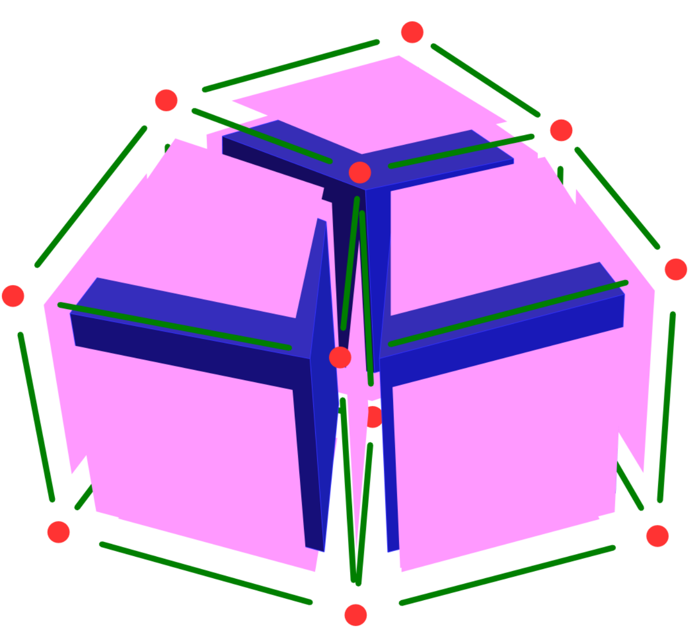
The domain $\overline{\Omega}$ is also referred to as multi-patch volume, and the collection of all geometry mappings $\boldsymbol{F}^{(i)}$ , $i\in\mathcal{I}_{\Omega}$ , is called the geometry of the multi-patch volume $\overline{\Omega}$ . An example of a three-patch volume $\overline{\Omega}$ with their individual patches $\Omega^{(i)}$ , $i\in\{1,2,3\}$ , and with their corresponding geometry mappings $\boldsymbol{F}^{(i)}$ , as well as the decomposition of the three-patch volume into the single patches $\Omega^{(i)}$ , $i\in\mathcal{I}_{\Omega}$ , faces $\Gamma^{(i)}$ , $i\in\mathcal{I}_{\Gamma}$ , edges $\Sigma^{(i)}$ , $i\in\mathcal{I}_{\Sigma}$ , and vertices $\Xi^{(i)}$ , $i\in\mathcal{I}_{\Xi}$ , is shown in Fig. 1.

Refer to caption — Figure 1: Left: A trilinear multi-patch volume $\overline{\Omega}$ with three patches $\Omega^{(i)}$ , $i\in\{1,2,3\}$ , and with their associated geometry mappings $\boldsymbol{F}^{(i)}$ . Right: The decomposition of the multi-patch volume $\overline{\Omega}$ into the single patches $\Omega^{(i)}$ (blue), faces $\Gamma^{(i)}$ (pink), edges $\Sigma^{(i)}$ (green) and vertices $\Xi^{(i)}$ (red).

2.2 The concept of $C^{1}$ isogeometric spline spaces for multi-patch volumes

Let $p\geq 3$ , $1\leq r\leq p-2$ and $k\geq 0$ . We denote by $\mathcal{S}_{h}^{p,r}$ the univariate spline space of degree $p$ and regularity $r$ on a uniform mesh of size $h=\frac{1}{k+1}$ over the unit interval $[0,1]$ , where $k+1$ is the number of spline elements. Moreover, let $\mathcal{S}_{h}^{\boldsymbol{p},\boldsymbol{r}}$ with $\boldsymbol{p}=(p,p)$ and $\boldsymbol{r}=(r,r)$ or $\boldsymbol{p}=(p,p,p)$ and $\boldsymbol{r}=(r,r,r)$ be the bivariate or trivariate tensor-product spline space $\mathcal{S}_{h}^{p,r}\times\mathcal{S}_{h}^{p,r}$ or $\mathcal{S}_{h}^{p,r}\times\mathcal{S}_{h}^{p,r}\times\mathcal{S}_{h}^{p,r}$ over the unit square $[0,1]^{2}$ or the unit cube $[0,1]^{3}$ , respectively. We denote by $N_{j}^{p,r}$ , $j\in\mathbb{I}=\{0,1,\ldots,n-1\}$ , the B-splines of the univariate spline space $\mathcal{S}_{h}^{p,r}$ , where $n$ is the dimension of the spline space $\mathcal{S}_{h}^{p,r}$ , i.e. $n=\dim\mathcal{S}_{h}^{p,r}=p+1+k(p-r)$ , and we denote by $N_{j_{1},j_{2}}^{\boldsymbol{p},\boldsymbol{r}}=N_{j_{1}}^{p,r}N_{j_{2}}^{p,r}$ , $j_{1},j_{2}\in\mathbb{I}$ , and $N_{j_{1},j_{2},j_{3}}^{\boldsymbol{p},\boldsymbol{r}}=N_{j_{1}}^{p,r}N_{j_{2}}^{p,r}N_{j_{3}}^{p,r}$ , $j_{1},j_{2},j_{3}\in\mathbb{I}$ , the tensor-product B-splines of the bivariate and trivariate spline space $\mathcal{S}_{h}^{\boldsymbol{p},\boldsymbol{r}}$ , respectively.

Note that the trilinear parameterization (3) of the geometry mappings $\boldsymbol{F}^{(i)}$ , $i\in\mathcal{I}_{\Omega}$ , trivially implies that $\boldsymbol{F}^{(i)}\in(\mathcal{S}_{h}^{\boldsymbol{p},\boldsymbol{r}})^{3}$ . Then, the space of isogeometric spline functions on the multi-patch volume $\overline{\Omega}$ (with respect to the spline space $\mathcal{S}_{h}^{\boldsymbol{p},\boldsymbol{r}}$ ) is defined as

\mathcal{V}=\left\{\phi\in L^{2}(\overline{\Omega})\;|\;\phi|_{\overline{\Omega^{(i)}}}\in\mathcal{S}_{h}^{\boldsymbol{p},\boldsymbol{r}}\circ(\boldsymbol{F}^{(i)})^{-1},\;i\in\mathcal{I}_{\Omega}\right\}.

Therefore, an isogeometric function $\phi\in\mathcal{V}$ possesses for each patch $\Omega^{(i)}$ , $i\in\mathcal{I}_{\Omega}$ , a spline function $f^{(i)}=\phi\circ\boldsymbol{F}^{(i)}$ of the form

f^{(i)}(\xi_{1},\xi_{2},\xi_{3})=\sum_{j_{1}=0}^{n-1}\sum_{j_{2}=0}^{n-1}\sum_{j_{3}=0}^{n-1}a_{j_{1},j_{2},j_{3}}^{(i)}N_{j_{1},j_{2},j_{3}}^{\boldsymbol{p},\boldsymbol{r}}(\xi_{1},\xi_{2},\xi_{3}),\quad(\xi_{1},\xi_{2},\xi_{3})\in[0,1]^{3},

with $a_{j_{1},j_{2},j_{3}}^{(i)}\in\mathbb{R}$ . We are interested in the $C^{1}$ subspace of $\mathcal{V}$ , which is given by

\mathcal{V}^{1}=\mathcal{V}\cap C^{1}(\overline{\Omega}).

The space $\mathcal{V}^{1}$ is fully characterized by the observation that an isogeometric function $\phi\in\mathcal{V}$ belongs to the space $\mathcal{V}^{1}$ if and only if for any two neighboring patches $\Omega^{(i_{0})}$ and $\Omega^{(i_{1})}$ , $i_{0},i_{1}\in\mathcal{I}_{\Omega}$ , with the common inner face $\overline{\Gamma^{(i)}}=\overline{\Omega^{(i_{0})}}\cap\overline{\Omega^{(i_{1})}}$ , $i\in\mathcal{I}_{\Gamma_{I}}$ , the associated graph patches $\left[\begin{array}[]{cc}\boldsymbol{F}^{(i_{0})}&\phi\circ\boldsymbol{F}^{(i_{0})}\end{array}\right]^{T}$ and $\left[\begin{array}[]{cc}\boldsymbol{F}^{(i_{1})}&\phi\circ\boldsymbol{F}^{(i_{1})}\end{array}\right]^{T}$ are $G^{1}$ -continuous, cf. [5, 14]. The $C^{1}$ continuity condition of an isogeometric function $\phi\in\mathcal{V}$ has been studied in detail for the two-patch case in [7], and will be recalled in the next section.

3 $C^{1}$ continuity condition

We present the $C^{1}$ smoothness condition of an isogeometric function $\phi\in\mathcal{V}$ , which has been already considered for the case of a two-patch volume in [7], and which can be also used in this work to study the $C^{1}$ isogeometric spline space $\mathcal{V}^{1}$ and to generate a basis for the space $\mathcal{V}^{1}$ over any possible configuration of a trilinear multi-patch volume $\overline{\Omega}$ . Firstly, we will introduce some required assumptions, definitions and concepts.

3.1 Assumptions, definitions and concepts

Let $\Gamma^{(i)}$ , $i\in\mathcal{I}_{\Gamma_{I}}$ , be an inner face with two neighboring patches $\Omega^{(i_{0})}$ and $\Omega^{(i_{1})}$ , $i_{0},i_{1}\in\mathcal{I}_{\Omega}$ , i.e. $\overline{\Gamma^{(i)}}=\overline{\Omega^{(i_{0})}}\cap\overline{\Omega^{(i_{1})}}$ . Then, we will assume throughout the paper and without loss of generality that the two associated geometry mappings $\boldsymbol{F}^{(i_{0})}$ and $\boldsymbol{F}^{(i_{1})}$ are (re)parameterized in such a way that the common inner face $\overline{\Gamma^{(i)}}$ is given by

\boldsymbol{F}^{(i_{0})}(0,t_{1},t_{2})=\boldsymbol{F}^{(i_{1})}(t_{1},0,t_{2}),\quad(t_{1},t_{2})\in[0,1]^{2},

(4)

and that the $12$ different vertices of the two-patch volume $\overline{\Omega^{(i_{0})}}\cup\overline{\Omega^{(i_{1})}}$ are labeled as $\Xi^{(i_{0})},\Xi^{(i_{1})},\ldots,$ $\Xi^{(i_{11})}$ , cf. Figure 2. We also say that the two geometry mappings $\boldsymbol{F}^{(i_{0})}$ and $\boldsymbol{F}^{(i_{1})}$ are given in standard form with respect to their common inner face $\Gamma^{(i)}$ when they fulfill (4).

Figure 2: For any inner face

\Gamma^{(i)}

i\in\mathcal{I}_{\Gamma_{I}}

, between the two neighboring patches

\Omega^{(i_{0})}

and

\Omega^{(i_{1})}

i_{0},i_{1}\in\mathcal{I}_{\Omega}

, we assume that the common inner face

\Gamma^{(i)}

is parameterized via the geometry mappings

\boldsymbol{F}^{(i_{0})}

and

\boldsymbol{F}^{(i_{1})}

as shown, and that the

12

different vertices are labeled as visualized.

We define bivariate functions $\alpha^{(i,i_{0})},\alpha^{(i,i_{1})},\beta^{(i)},\gamma^{(i)}:[0,1]^{2}\rightarrow\mathbb{R}$ by

\begin{split}\alpha^{(i,i_{0})}(t_{1},t_{2})=\lambda\det\left(\partial_{1}\boldsymbol{F}^{(i_{0})}(0,t_{1},t_{2}),\partial_{2}\boldsymbol{F}^{(i_{0})}(0,t_{1},t_{2}),\partial_{3}\boldsymbol{F}^{(i_{0})}(0,t_{1},t_{2})\right),\\ \alpha^{(i,i_{1})}(t_{1},t_{2})=\lambda\det\left(\partial_{1}\boldsymbol{F}^{(i_{1})}(t_{1},0,t_{2}),\partial_{2}\boldsymbol{F}^{(i_{1})}(t_{1},0,t_{2}),\partial_{3}\boldsymbol{F}^{(i_{1})}(t_{1},0,t_{2})\right),\\ \beta^{(i)}(t_{1},t_{2})=\lambda\det\left(\partial_{2}\boldsymbol{F}^{(i_{1})}(t_{1},0,t_{2}),\partial_{3}\boldsymbol{F}^{(i_{1})}(t_{1},0,t_{2}),\partial_{1}\boldsymbol{F}^{(i_{0})}(0,t_{1},t_{2})\right),\\ \gamma^{(i)}(t_{1},t_{2})=\lambda\det\left(\partial_{1}\boldsymbol{F}^{(i_{1})}(t_{1},0,t_{2}),\partial_{2}\boldsymbol{F}^{(i_{1})}(t_{1},0,t_{2}),\partial_{1}\boldsymbol{F}^{(i_{0})}(0,t_{1},t_{2})\right),\end{split}

(5)

where $\lambda\in(0,\infty)$ is given by minimizing the term

||\alpha^{(i_{0})}-1||^{2}_{L_{2}}+||\alpha^{(i_{1})}-1||^{2}_{L_{2}},

and which satisfy

	$\displaystyle\alpha^{(i,i_{0})}(t_{1},t_{2})\partial_{2}\boldsymbol{F}^{(i_{1})}(t_{1},0,t_{2})+\alpha^{(i,i_{1})}(t_{1},t_{2})\partial_{1}\boldsymbol{F}^{(i_{0})}(0,t_{1},t_{2})-$
	$\displaystyle\beta^{(i)}(t_{1},t_{2})\partial_{1}\boldsymbol{F}^{(i_{1})}(t_{1},0,t_{2})-\gamma^{(i)}(t_{1},t_{2})\partial_{3}\boldsymbol{F}^{(i_{1})}(t_{1},0,t_{2})=\boldsymbol{0}$

for $(t_{1},t_{2})\in[0,1]^{2}$ , cf. [7]. Since the geometry mappings $\boldsymbol{F}^{(i_{0})}$ and $\boldsymbol{F}^{(i_{1})}$ are trilinear, non-singular parameterizations, the functions $\alpha^{(i,i_{0})}$ , $\alpha^{(i,i_{1})}$ , $\beta^{(i)}$ and $\gamma^{(i)}$ are bivariate polynomials of bidegree $(2,2)$ , $(2,2)$ , $(3,2)$ and $(2,3)$ , respectively, and the functions $\alpha^{(i,i_{0})}$ and $\alpha^{(i,i_{1})}$ further fulfill

\alpha^{(i,i_{0})}(t_{1},t_{2})>0\mbox{ and }\alpha^{(i,i_{1})}(t_{1},t_{2})>0,\mbox{ }(t_{1},t_{2})\in[0,1]^{2}.

It was also shown in [7], that in case of a non-planar face $\Gamma^{(i)}$ , there exist bilinear polynomial functions $\beta^{(i,i_{0})},\beta^{(i,i_{1})},\gamma^{(i,i_{0})},\gamma^{(i,i_{1})}:[0,1]^{2}\rightarrow\mathbb{R}$ given by

\begin{split}\beta^{(i,i_{0})}(t_{1},t_{2})=\frac{\det(\Xi^{(i_{6})}-\Xi^{(i_{2})},\Xi^{(i_{0})}-\Xi^{(i_{4})},\partial_{1}\boldsymbol{F}^{(i_{0})}(0,t_{1},t_{2}))}{\text{vol}^{(i)}},\\ \beta^{(i,i_{1})}(t_{1},t_{2})=\frac{\det(\Xi^{(i_{6})}-\Xi^{(i_{2})},\Xi^{(i_{0})}-\Xi^{(i_{4})},\partial_{2}\boldsymbol{F}^{(i_{1})}(t_{1},0,t_{2}))}{\text{vol}^{(i)}},\\ \end{split}

and

\begin{split}\gamma^{(i,i_{0})}(t_{1},t_{2})=\frac{\det(\Xi^{(i_{6})}-\Xi^{(i_{4})},\Xi^{(i_{2})}-\Xi^{(i_{0})},\partial_{1}\boldsymbol{F}^{(i_{0})}(0,t_{1},t_{2}))}{\text{vol}^{(i)}},\\ \gamma^{(i,i_{1})}(t_{1},t_{2})=\frac{\det(\Xi^{(i_{6})}-\Xi^{(i_{4})},\Xi^{(i_{2})}-\Xi^{(i_{0})},\partial_{2}\boldsymbol{F}^{(i_{1})}(t_{1},0,t_{2}))}{\text{vol}^{(i)}},\\ \end{split}

respectively, which satisfy

\beta^{(i)}(t_{1},t_{2})=\beta^{(i,i_{0})}(t_{1},t_{2})\alpha^{(i,i_{1})}(t_{1},t_{2})+\beta^{(i,i_{1})}(t_{1},t_{2})\alpha^{(i,i_{0})}(t_{1},t_{2})

(7)

and

\gamma^{(i)}(t_{1},t_{2})=\gamma^{(i,i_{0})}(t_{1},t_{2})\alpha^{(i,i_{1})}(t_{1},t_{2})+\gamma^{(i,i_{1})}(t_{1},t_{2})\alpha^{(i,i_{0})}(t_{1},t_{2}),

(8)

where $\text{vol}^{(i)}$ is the volume of the rectangular solid spanned by the three vectors $\Xi^{(i_{2})}-\Xi^{(i_{0})}$ , $\Xi^{(i_{4})}-\Xi^{(i_{0})}$ and $\Xi^{(i_{6})}-\Xi^{(i_{0})}$ , i.e.

\text{vol}^{(i)}=\det(\Xi^{(i_{2})}-\Xi^{(i_{0})},\Xi^{(i_{4})}-\Xi^{(i_{0})},\Xi^{(i_{6})}-\Xi^{(i_{0})}),

with the four vertices $\Xi^{(i_{0})}$ , $\Xi^{(i_{2})}$ , $\Xi^{(i_{4})}$ and $\Xi^{(i_{6})}$ of the common face $\Gamma^{(i)}$ . In addition, the functions $\alpha^{(i,i_{0})}$ and $\alpha^{(i,i_{1})}$ can be written as

\alpha^{(i,i_{0})}(t_{1},t_{2})=\lambda\,\text{vol}^{(i)}\left(\delta^{(i,i_{0})}(t_{1},t_{2})-t_{1}\gamma^{(i,i_{0})}(t_{1},t_{2})-t_{2}\beta^{(i,i_{0})}(t_{1},t_{2})\right)

and

\alpha^{(i,i_{1})}(t_{1},t_{2})=-\lambda\,\text{vol}^{(i)}\left(\delta^{(i,i_{1})}(t_{1},t_{2})-t_{1}\gamma^{(i,i_{1})}(t_{1},t_{2})-t_{2}\beta^{(i,i_{1})}(t_{1},t_{2})\right),

with bilinear polynomial functions

\delta^{(i,i_{0})}(t_{1},t_{2})=\frac{\det(\Xi^{(i_{2})}-\Xi^{(i_{0})},\Xi^{(i_{4})}-\Xi^{(i_{0})},\partial_{1}\boldsymbol{F}^{(i_{0})}(0,t_{1},t_{2}))}{\text{vol}^{(i)}}

and

\delta^{(i,i_{1})}(t_{1},t_{2})=\frac{\det(\Xi^{(i_{2})}-\Xi^{(i_{0})},\Xi^{(i_{4})}-\Xi^{(i_{0})},\partial_{2}\boldsymbol{F}^{(i_{1})}(t_{1},0,t_{2}))}{\text{vol}^{(i)}}.

In case of a boundary face $\Gamma^{(i)}$ , $i\in\mathcal{I}_{\Gamma_{B}}$ , which is contained in the closure of the patch $\Omega^{(i_{0})}$ , $i_{0}\in\mathcal{I}_{\Omega}$ , i.e. $\Gamma^{(i)}\subset\overline{\Omega^{(i_{0})}}$ , we will similarly assume as in the case of an inner face shown in Fig. 2, that the corresponding geometry mapping $\boldsymbol{F}^{(i_{0})}$ is (re)parameterized in such a way that the face $\overline{\Gamma^{(i)}}$ is given by

\boldsymbol{F}^{(i_{0})}(0,t_{1},t_{2}),\mbox{ }(t_{1},t_{2})\in[0,1]^{2},

(9)

and that the $8$ vertices of the patch $\overline{\Omega^{(i_{0})}}$ are labeled as $\Xi^{(i_{0})},\Xi^{(i_{1})},\ldots,\Xi^{(i_{7})}$ . We say that the geometry mapping $\boldsymbol{F}^{(i_{0})}$ is given in standard form with respect to its boundary face $\Gamma^{(i)}$ when it fulfills (9).

Below, inspired by the work in [7] for the case of trilinearly parameterized two-patch volumes, we will assume that the considered trilinear multi-patch volumes $\overline{\Omega}$ satisfy the following assumption:

Assumption 1.

Each inner face $\Gamma^{(i)}$ , $i\in\mathcal{I}_{\Gamma_{I}}$ , is non-planar, and its functions $\alpha^{(i,i_{0})}$ , $\alpha^{(i,i_{1})}$ , $\beta^{(i)}$ and $\gamma^{(i)}$ possess full bidegrees $(2,2)$ , $(2,2)$ , $(3,2)$ and $(2,3)$ , respectively, its functions $\beta^{(i)}$ and $\gamma^{(i)}$ have no roots in the values $(j_{1}\,h,j_{2}\,h)$ , $j_{1},j_{2}=1,2,\ldots,k$ , and the greatest common divisor of its functions $\alpha^{(i,i_{0})}$ and $\alpha^{(i,i_{1})}$ is a constant function.

Note that each trilinear multi-patch volume $\overline{\Omega}$ , which does not satisfy Assumption 1, can be enforced to fulfill the assumption by slightly disturbing some of the values of their vertices $\Xi^{(i)}$ , $i\in\mathcal{I}_{\Xi}$ .

3.2 $C^{1}$ continuity condition across inner faces

As already mentioned in Section 2.2, an isogeometric function $\phi\in\mathcal{V}$ belongs to the $C^{1}$ isogeometric spline space $\mathcal{V}^{1}$ if and only if for any two neighboring patches $\Omega^{(i_{0})}$ and $\Omega^{(i_{1})}$ , $i_{0},i_{1}\in\mathcal{I}_{\Omega}$ , with the common inner face $\overline{\Gamma^{(i)}}=\overline{\Omega^{(i_{0})}}\cap\overline{\Omega^{(i_{1})}}$ , $i\in\mathcal{I}_{\Gamma_{I}}$ , the associated graph patches $\left[\begin{array}[]{cc}\boldsymbol{F}^{(i_{0})}&\phi\circ\boldsymbol{F}^{(i_{0})}\end{array}\right]^{T}$ and $\left[\begin{array}[]{cc}\boldsymbol{F}^{(i_{1})}&\phi\circ\boldsymbol{F}^{(i_{1})}\end{array}\right]^{T}$ meet with $G^{1}$ continuity. Let us consider two such neighboring patches $\Omega^{(i_{0})}$ and $\Omega^{(i_{1})}$ , $i_{0},i_{1}\in\mathcal{I}_{\Omega}$ , and let us assume without loss of generality that the two corresponding geometry mappings $\boldsymbol{F}^{(i_{0})}$ and $\boldsymbol{F}^{(i_{1})}$ are given in standard form (4) with respect to the common inner face $\overline{\Gamma^{(i)}}$ , $i\in\mathcal{I}_{\Gamma_{I}}$ . We further consider an isogeometric function $\phi\in\mathcal{V}$ , and recall that we denote by $f^{(i_{0})}$ and $f^{(i_{1})}$ its associated spline functions $\phi\circ\boldsymbol{F}^{(i_{0})}$ and $\phi\circ\boldsymbol{F}^{(i_{1})}$ , respectively. Then, the two graph patches $\left[\begin{array}[]{cc}\boldsymbol{F}^{(i_{0})}&f^{(i_{0})}\end{array}\right]^{T}$ and $\left[\begin{array}[]{cc}\boldsymbol{F}^{(i_{1})}&f^{(i_{1})}\end{array}\right]^{T}$ are $G^{1}$ -continuous if

\left[\begin{array}[]{c}\boldsymbol{F}^{(i_{0})}(0,t_{1},t_{2})\\ f^{(i_{0})}(0,t_{1},t_{2})\end{array}\right]=\left[\begin{array}[]{c}\boldsymbol{F}^{(i_{1})}(t_{1},0,t_{2})\\ f^{(i_{1})}(t_{1},0,t_{2})\end{array}\right],\quad(t_{1},t_{2})\in[0,1]^{2},

and if there exist bivariate functions $\widetilde{\alpha}^{(i,i_{0})},\widetilde{\alpha}^{(i,i_{1})},\widetilde{\beta}^{(i)},\widetilde{\gamma}^{(i)}:[0,1]^{2}\rightarrow\mathbb{R}$ with $\widetilde{\alpha}^{(i,i_{0})}\widetilde{\alpha}^{(i,i_{1})}>0$ , such that

	$\displaystyle\widetilde{\alpha}^{(i,i_{0})}(t_{1},t_{2})\left[\begin{array}[]{c}\partial_{2}\boldsymbol{F}^{(i_{1})}(t_{1},0,t_{2})\\ \partial_{2}f^{(i_{1})}(t_{1},0,t_{2})\end{array}\right]+\widetilde{\alpha}^{(i,i_{1})}(t_{1},t_{2})\left[\begin{array}[]{c}\partial_{1}\boldsymbol{F}^{(i_{0})}(0,t_{1},t_{2})\\ \partial_{1}f^{(i_{0})}(0,t_{1},t_{2})\end{array}\right]-$
	$\displaystyle\widetilde{\beta}^{(i)}(t_{1},t_{2})\left[\begin{array}[]{c}\partial_{1}\boldsymbol{F}^{(i_{1})}(t_{1},0,t_{2})\\ \partial_{1}f^{(i_{1})}(t_{1},0,t_{2})\end{array}\right]-\widetilde{\gamma}^{(i)}(t_{1},t_{2})\left[\begin{array}[]{c}\partial_{3}\boldsymbol{F}^{(i_{1})}(t_{1},0,t_{2})\\ \partial_{3}f^{(i_{1})}(t_{1},0,t_{2})\end{array}\right]=\boldsymbol{0},$

for $(t_{1},t_{2})\in[0,1]^{2}$ . Since the geometry mappings $\boldsymbol{F}^{(i_{0})}$ and $\boldsymbol{F}^{(i_{1})}$ are given, the first three coordinate rows in equation () uniquely determine the functions $\widetilde{\alpha}^{(i,i_{0})}$ , $\widetilde{\alpha}^{(i,i_{1})}$ , $\widetilde{\beta}^{(i)}$ and $\widetilde{\gamma}^{(i)}$ up to a common function $\widetilde{\lambda}:[0,1]^{2}\rightarrow\mathbb{R}$ . Without loss of generality, we choose the functions $\widetilde{\alpha}^{(i,i_{0})}$ , $\widetilde{\alpha}^{(i,i_{1})}$ , $\widetilde{\beta}^{(i)}$ and $\widetilde{\gamma}^{(i)}$ as the functions $\alpha^{(i,i_{0})}$ , $\alpha^{(i,i_{1})}$ , $\beta^{(i)}$ and $\gamma^{(i)}$ defined in equation (5), which fulfill the first three coordinate rows in equation () , cf. equation (). Therefore, the isogeometric function $\phi$ is $C^{1}$ across the inner face $\overline{\Gamma^{(i)}}$ if and only if

f^{(i_{0})}(0,t_{1},t_{2})=f^{(i_{1})}(t_{1},0,t_{2}),\mbox{ }(t_{1},t_{2})\in[0,1]^{2},

(19)

and

	$\displaystyle\alpha^{(i,i_{0})}(t_{1},t_{2})\partial_{2}f^{(i_{1})}(t_{1},0,t_{2})+\alpha^{(i,i_{1})}(t_{1},t_{2})\partial_{1}f^{(i_{0})}(0,t_{1},t_{2})-$
	$\displaystyle\beta^{(i)}(t_{1},t_{2})\partial_{1}f^{(i_{1})}(t_{1},0,t_{2})-\gamma^{(i)}(t_{1},t_{2})\partial_{3}f^{(i_{1})}(t_{1},0,t_{2})=0,$

for $(t_{1},t_{2})\in[0,1]^{2}$ , and the function $\phi$ is globally $C^{1}$ on $\overline{\Omega}$ , i.e. $\phi\in\mathcal{V}^{1}$ , if and only if the pull-back of the function $\phi$ satisfies equations (19) and () for any inner face $\overline{\Gamma^{(j)}}$ , $j\in\mathcal{I}_{\Gamma_{I}}$ .

Let us consider the $C^{1}$ continuity condition () of the isogeometric function $\phi$ across the inner face $\overline{\Gamma^{(i)}}$ in more detail. By using relations (7), (8) and (19), the condition () is equivalent to

	$\displaystyle\frac{\partial_{1}f^{(i_{0})}(0,t_{1},t_{2})-\beta^{(i,i_{0})}(t_{1},t_{2})\partial_{2}f^{(i_{0})}(0,t_{1},t_{2})-\gamma^{(i,i_{0})}(t_{1},t_{2})\partial_{3}f^{(i_{0})}(0,t_{1},t_{2})}{\alpha^{(i,i_{0})}(t_{1},t_{2})}=$
	$\displaystyle-\frac{\partial_{2}f^{(i_{1})}(t_{1},0,t_{2})-\beta^{(i,i_{1})}(t_{1},t_{2})\partial_{1}f^{(i_{1})}(t_{1},0,t_{2})-\gamma^{(i,i_{1})}(t_{1},t_{2})\partial_{3}f^{(i_{1})}(t_{1},0,t_{2})}{\alpha^{(i,i_{1})}(t_{1},t_{2})}.$

Let $f_{0}:[0,1]^{2}\rightarrow\mathbb{R}$ and $f_{1}:[0,1]^{2}\rightarrow\mathbb{R}$ be the two bivariate functions, which are determined by the equally valued terms in equation (19) and (), respectively. While the function $f_{0}$ is just the trace of the function $\phi$ at the common inner face $\overline{\Gamma^{(i)}}$ , i.e.

f_{0}(t_{1},t_{2})=\phi\circ\boldsymbol{F}^{(i_{0})}(0,t_{1},t_{2})=\phi\circ\boldsymbol{F}^{(i_{1})}(t_{1},0,t_{2}),\quad(t_{1},t_{2})\in[0,1]^{2},

the function $f_{1}$ is the directional derivative of $\phi$ with respect to the transversal direction $\boldsymbol{d}^{(i)}$ at the common inner face $\overline{\Gamma^{(i)}}$ , i.e.

f_{1}(t_{1},t_{2})=\nabla\phi\cdot\boldsymbol{d}^{(i)}\circ\boldsymbol{F}^{(i_{0})}(0,t_{1},t_{2})=\nabla\phi\cdot\boldsymbol{d}^{(i)}\circ\boldsymbol{F}^{(i_{1})}(t_{1},0,t_{2}),\quad(t_{1},t_{2})\in[0,1]^{2},

with $\boldsymbol{d}^{(i)}=\boldsymbol{d}^{(i,i_{0})}=\boldsymbol{d}^{(i,i_{1})}$ on $\overline{\Gamma^{(i)}}$ given as

\boldsymbol{d}^{(i,i_{0})}\circ\boldsymbol{F}^{(i_{0})}(0,t_{1},t_{2})=\text{grad}\boldsymbol{F}^{(i_{0})}(0,t_{1},t_{2})\cdot\left[\begin{array}[]{ccc}-\beta^{(i,i_{0})}(t_{1},t_{2})&-\gamma^{(i,i_{0})}(t_{1},t_{2})&1\end{array}\right]^{T}\frac{1}{\alpha^{(i,i_{0})}(t_{1},t_{2})}

and

\boldsymbol{d}^{(i,i_{1})}\circ\boldsymbol{F}^{(i_{1})}(t_{1},0,t_{2})=\text{grad}\boldsymbol{F}^{(i_{1})}(t_{1},0,t_{2})\cdot\left[\begin{array}[]{ccc}\beta^{(i,i_{1})}(t_{1},t_{2})&\gamma^{(i,i_{1})}(t_{1},t_{2})&-1\end{array}\right]^{T}\frac{1}{\alpha^{(i,i_{1})}(t_{1},t_{2})},

cf. [7]. The use of the functions $f_{0}$ and $f_{1}$ directly implies that

f^{(i_{0})}(0,t_{1},t_{2})=f^{(i_{1})}(t_{1},0,t_{2})=f_{0}(t_{1},t_{2}),

\partial_{1}f^{(i_{0})}(0,t_{1},t_{2})=\beta^{(i,i_{0})}(t_{1},t_{2})\partial_{1}f_{0}(t_{1},t_{2})+\gamma^{(i,i_{0})}(t_{1},t_{2})\partial_{2}f_{0}(t_{1},t_{2})+\alpha^{(i,i_{0})}(t_{1},t_{2})f_{1}(t_{1},t_{2}),

and

\partial_{2}f^{(i_{1})}(t_{1},0,t_{2})=\beta^{(i,i_{1})}(t_{1},t_{2})\partial_{1}f_{0}(t_{1},t_{2})+\gamma^{(i,i_{1})}(t_{1},t_{2})\partial_{2}f_{0}(t_{1},t_{2})-\alpha^{(i,i_{1})}(t_{1},t_{2})f_{1}(t_{1},t_{2}).

Then, the Taylor expansion of $f^{(i_{0})}=\phi\circ\boldsymbol{F}^{(i_{0})}$ at $(\xi_{1},\xi_{2},\xi_{3})=(0,\xi_{2},\xi_{3})$ , and the Taylor expansion of $f^{(i_{1})}=\phi\circ\boldsymbol{F}^{(i_{1})}$ at $(\xi_{1},\xi_{2},\xi_{3})=(\xi_{1},0,\xi_{3})$ is given by

	$\displaystyle f^{(i_{0})}(\xi_{1},\xi_{2},\xi_{3})$	$\displaystyle=$	$\displaystyle f_{0}(\xi_{2},\xi_{3})+\big(\beta^{(i,i_{0})}(\xi_{2},\xi_{3})\partial_{1}f_{0}(\xi_{2},\xi_{3})+$
			$\displaystyle\gamma^{(i,i_{0})}(\xi_{2},\xi_{3})\partial_{2}f_{0}(\xi_{2},\xi_{3})+\alpha^{(i,i_{0})}(\xi_{2},\xi_{3})f_{1}(\xi_{2},\xi_{3})\big)\xi_{1}+\mathcal{O}(\xi_{1}^{2}),$

and by

	$\displaystyle f^{(i_{1})}(\xi_{1},\xi_{2},\xi_{3})$	$\displaystyle=$	$\displaystyle f_{0}(\xi_{1},\xi_{3})+\big(\beta^{(i,i_{1})}(\xi_{1},\xi_{3})\partial_{1}f_{0}(\xi_{1},\xi_{3})+$
			$\displaystyle\gamma^{(i,i_{1})}(\xi_{1},\xi_{3})\partial_{2}f_{0}(\xi_{1},\xi_{3})-\alpha^{(i,i_{1})}(\xi_{1},\xi_{3})f_{1}(\xi_{1},\xi_{3})\big)\xi_{2}+\mathcal{O}(\xi_{2}^{2}),$

respectively, cf. [7]. The representations () and () of an isogeometric function $\phi\in\mathcal{V}^{1}$ along an inner face $\overline{\Gamma^{(i)}}$ , $i\in\mathcal{I}_{\Gamma_{I}}$ , will be used in the next sections to study and to design the $C^{1}$ isogeometric spline space $\mathcal{V}^{1}$ for trilinear multi-patch volumes $\overline{\Omega}$ .

4 Design and study of $C^{1}$ isogeometric spline spaces

In [7], the $C^{1}$ isogeometric spline space $\mathcal{V}^{1}$ for the case of a trilinear two-patch volume $\overline{\Omega}$ was studied, and a basis for the space $\mathcal{V}^{1}$ was constructed. This basis consists of $C^{1}$ functions, which possess simple explicit representations and have small local supports, and will be used in this and in the next section as a tool for the investigation of the $C^{1}$ isogeometric spline space $\mathcal{V}^{1}$ for the case of a trilinear multi-patch volume $\overline{\Omega}$ . More precisely, we will present in this section for the trilinear multi-patch volumes $\overline{\Omega}$ a general framework for design of the corresponding $C^{1}$ isogeometric spline space $\mathcal{V}^{1}$ and of an associated basis, and will then focus in the next section on a more detailed study for a particular subclass of trilinearly parameterized multi-patch volumes $\overline{\Omega}$ . Before, we will introduce some needed additional notations and definitions, and will briefly recall the construction [7] for the two-patch case.

4.1 Preliminaries

Let $\mathbb{I}_{0}=\{0,1,\ldots,n_{0}-1\}$ and $\mathbb{I}_{1}=\{0,1,\ldots,n_{1}-1\}$ with $n_{0}=\dim\mathcal{S}_{h}^{p,r+1}=p+1+k(p-r-1)$ and $n_{1}=\dim\mathcal{S}_{h}^{p-2,r}=p-1+k(p-r-2)$ be the index sets of the univariate B-splines $N_{j}^{p,r+1}$ and $N_{j}^{p-2,r}$ of the spline spaces $\mathcal{S}_{h}^{p,r+1}$ and $\mathcal{S}_{h}^{p-2,r}$ , respectively. In addition, let $R_{j}^{p,r+1}:[0,1]\rightarrow\mathbb{R}$ , $j\in\mathbb{I}_{0}$ , be the spline functions defined by

R_{j}^{p,r+1}(\xi)=\begin{cases}-hN_{j}^{p-1,r}(\xi)&\mbox{if }j=0,\\ h\,(N_{j-1}^{p-1,r}(\xi)-N_{j}^{p-1,r}(\xi))\;&\mbox{if }j\in\mathbb{I}_{0}\setminus\{0,n_{0}-1\},\\ hN_{j-1}^{p-1,r}(\xi)\;&\mbox{if }j=n_{0}-1,\end{cases}

and let $R_{j_{1},j_{2}}^{\boldsymbol{p},\boldsymbol{r+1}}$ be the tensor-product spline functions $R_{j_{1},j_{2}}^{\boldsymbol{p},\boldsymbol{r+1}}=R_{j_{1}}^{p,r+1}R_{j_{2}}^{p,r+1}$ , $j_{1},j_{2}\in\mathbb{I}_{0}$ . We further denote by $M_{j}^{p,r}:[0,1]\rightarrow\mathbb{R}$ , $j=0,1$ , the basis transformation of the B-splines $N_{j}^{p,r}$ , $j=0,1$ , given by

M_{0}^{p,r}(\xi)=N_{0}^{p,r}(\xi)+N_{1}^{p,r}(\xi)\quad{\rm and}\quad M_{1}^{p,r}(\xi)=\frac{h}{p}N_{1}^{p,r}(\xi),

which fulfill $\partial_{\xi}^{i}M_{j}^{p,r}(0)=\delta_{j}^{i}$ , $i=0,1$ , where $\delta_{j}^{i}$ is the Kronecker delta.

Recall that for any inner face $\Gamma^{(i)}$ , $i\in\mathcal{I}_{\Gamma_{I}}$ , with the two neighboring patches $\Omega^{(i_{0})}$ and $\Omega^{(i_{1})}$ , $i_{0},i_{1}\in\mathcal{I}_{\Omega}$ , i.e. $\overline{\Gamma^{(i)}}=\overline{\Omega^{(i_{0})}}\cap\overline{\Omega^{(i_{1})}}$ , we can assume that the two associated geometry mappings $\boldsymbol{F}^{(i_{0})}$ and $\boldsymbol{F}^{(i_{1})}$ can be reparameterized (if necessary) to be in standard form (4). Similarly, for any boundary face $\Gamma^{(i)}$ , $i\in\mathcal{I}_{\Gamma_{B}}$ , which is contained in the closure of the patch $\Omega^{(i_{0})}$ , $i_{0}\in\mathcal{I}_{\Omega}$ , i.e. $\Gamma^{(i)}\subset\overline{\Omega^{(i_{0})}}$ , the associated geometry mapping $\boldsymbol{F}^{(i_{0})}$ can be assumed to be in standard form (9).

We define on the trilinear multi-patch volume $\overline{\Omega}$ for each patch $\Omega^{(i)}$ , $i\in\mathcal{I}_{\Omega}$ , the isogeometric functions $\phi_{\Omega^{(i)};j_{1},j_{2},j_{3}}$ , $i=0,1$ , $j_{1},j_{2},j_{3}\in\mathbb{I}$ , for each boundary face $\Gamma^{(i)}$ , $i\in\mathcal{I}_{\Gamma_{B}}$ , the isogeometric functions $\phi_{\Gamma^{(i)};j_{1},j_{2},j_{3}}$ , $j_{1}=0,1$ , $j_{2},j_{3}\in\mathbb{I}$ , and for each inner face $\Gamma^{(i)}$ , $i\in\mathcal{I}_{\Gamma_{I}}$ , the isogeometric functions $\phi_{\Gamma^{(i)};j_{1},j_{2},j_{3}}$ , $j_{1}=0,1$ , $j_{2},j_{3}\in\mathbb{I}_{j_{1}}$ , whose spline functions $f^{(\tau)}_{\Omega^{(i)};j_{1},j_{2},j_{3}}=\phi_{\Omega^{(i)};j_{1},j_{2},j_{3}}\circ\boldsymbol{F}^{(\tau)}$ and $f^{(\tau)}_{\Gamma^{(i)};j_{1},j_{2},j_{3}}=\phi_{\Gamma^{(i)};j_{1},j_{2},j_{3}}\circ\boldsymbol{F}^{(\tau)}$ for $\tau\in\mathcal{I}_{\Omega}$ , possess the form

f^{(\tau)}_{\Omega^{(i)};j_{1},j_{2},j_{3}}(\xi_{1},\xi_{2},\xi_{3})=\begin{cases}N_{j_{1},j_{2},j_{3}}^{\boldsymbol{p},\boldsymbol{r}}(\xi_{1},\xi_{2},\xi_{3})&\mbox{if }\tau=i,\\ 0&\mbox{otherwise},\end{cases}

f^{(\tau)}_{\Gamma^{(i)};j_{1},j_{2},j_{3}}(\xi_{1},\xi_{2},\xi_{3})=f^{(\tau)}_{\Omega^{(i_{0})};j_{1},j_{2},j_{3}}(\xi_{1},\xi_{2},\xi_{3}),

for $i\in\mathcal{I}_{\Gamma_{B}}$ , and

f^{(\tau)}_{\Gamma^{(i)};0,j_{2},j_{3}}(\xi_{1},\xi_{2},\xi_{3})=\begin{cases}\begin{array}[]{c}N_{j_{2},j_{3}}^{\boldsymbol{p},\boldsymbol{r+1}}(\xi_{2},\xi_{3})M_{0}^{p,r}(\xi_{1})+\big(\beta^{(i,i_{0})}(\xi_{2},\xi_{3})\partial_{1}N_{j_{2},j_{3}}^{\boldsymbol{p},\boldsymbol{r+1}}(\xi_{2},\xi_{3})+\\ \gamma^{(i,i_{0})}(\xi_{2},\xi_{3})\partial_{2}N_{j_{2},j_{3}}^{\boldsymbol{p},\boldsymbol{r+1}}(\xi_{2},\xi_{3})+\\ \alpha^{(i,i_{0})}(\xi_{2},\xi_{3})\frac{p}{\lambda\,\text{vol}^{(i)}}R_{j_{2},j_{3}}^{\boldsymbol{p},\boldsymbol{r+1}}(\xi_{2},\xi_{3})\big)M_{1}^{p,r}(\xi_{1}),\end{array}&$\hskip-11.38092pt $\mbox{if }\tau=i_{0},\\ \begin{array}[]{c}N_{j_{2},j_{3}}^{\boldsymbol{p},\boldsymbol{r+1}}(\xi_{1},\xi_{3})M_{0}^{p,r}(\xi_{2})+\big(\beta^{(i,i_{1})}(\xi_{1},\xi_{3})\partial_{1}N_{j_{2},j_{3}}^{\boldsymbol{p},\boldsymbol{r+1}}(\xi_{1},\xi_{3})+\\ \gamma^{(i,i_{1})}(\xi_{1},\xi_{3})\partial_{2}N_{j_{2},j_{3}}^{\boldsymbol{p},\boldsymbol{r+1}}(\xi_{1},\xi_{3})-\\ \alpha^{(i,i_{1})}(\xi_{1},\xi_{3})\frac{p}{\lambda\,\text{vol}^{(i)}}R_{j_{2},j_{3}}^{\boldsymbol{p},\boldsymbol{r+1}}(\xi_{1},\xi_{3})\big)M_{1}^{p,r}(\xi_{2}),\end{array}&$\hskip-11.38092pt $\mbox{if }\tau=i_{1},\\ \quad 0&$\hskip-17.07182pt $\mbox{otherwise},\end{cases}

f^{(\tau)}_{\Gamma^{(i)};1,j_{2},j_{3}}(\xi_{1},\xi_{2},\xi_{3})=\begin{cases}\alpha^{(i,i_{0})}(\xi_{2},\xi_{3})N_{j_{2},j_{3}}^{\boldsymbol{p-2},\boldsymbol{r}}(\xi_{2},\xi_{3})M_{1}^{p,r}(\xi_{1})&\mbox{if }\tau=i_{0},\\ -\alpha^{(i,i_{1})}(\xi_{1},\xi_{3})N_{j_{2},j_{3}}^{\boldsymbol{p-2},\boldsymbol{r}}(\xi_{1},\xi_{3})M_{1}^{p,r}(\xi_{2})&\mbox{if }\tau=i_{1},\\ 0&\mbox{otherwise},\end{cases}

for $i\in\mathcal{I}_{\Gamma_{I}}$ .

The functions $\phi_{\Omega^{(i)};j_{1},j_{2},j_{3}}$ , $i\in\mathcal{I}_{\Omega}$ , $j_{1},j_{2},j_{3}\in\mathbb{I}$ , are just the standard isogeometric spline functions, and are $C^{1}$ on $\overline{\Omega}$ , if they have vanishing values and gradients at all inner faces $\overline{\Gamma^{(\ell)}}$ , $\ell\in\mathcal{I}_{\Gamma_{I}}$ , i.e. $\phi_{\Omega^{(i)};j_{1},j_{2},j_{3}}(\overline{\Gamma^{(\ell)}})=0$ and $\nabla\phi_{\Omega^{(i)};j_{1},j_{2},j_{3}}(\overline{\Gamma^{(\ell)}})=\boldsymbol{0}$ . For $j_{1},j_{2},j_{3}\in\mathbb{I}\setminus\{0,1,n-2,n-1\}$ , it is guaranteed that the function $\phi_{\Omega^{(i)};j_{1},j_{2},j_{3}}$ belongs to the space $\mathcal{V}^{1}$ .

For a boundary face $\Gamma^{(i)}$ , $i\in\mathcal{I}_{\Gamma_{B}}$ , the functions $\phi_{\Gamma^{(i)};j_{1},j_{2},j_{3}}$ , $j_{1}=0,1$ , $j_{2},j_{3}\in\mathbb{I}$ , are again just the standard isogeometric spline functions, which are analogously as before $C^{1}$ on $\overline{\Omega}$ , if the functions possess vanishing values and gradients at all inner faces $\overline{\Gamma^{(\ell)}}$ , $\ell\in\mathcal{I}_{\Gamma_{I}}$ , i.e. $\phi_{\Gamma^{(i)};j_{1},j_{2},j_{3}}(\overline{\Gamma^{(\ell)}})=0$ and $\nabla\phi_{\Gamma^{(i)};j_{1},j_{2},j_{3}}(\overline{\Gamma^{(\ell)}})=\boldsymbol{0}$ . Now, the function $\phi_{\Gamma^{(i)};j_{1},j_{2},j_{3}}$ belongs in any case to the space $\mathcal{V}^{1}$ , if $j_{1}=0,1$ , $j_{2},j_{3}\in\mathbb{I}\setminus\{0,1,n-2,n-1\}$ .

For an inner face $\Gamma^{(i)}$ , $i\in\mathcal{I}_{\Gamma_{I}}$ , the functions $\phi_{\Gamma^{(i)};j_{1},j_{2},j_{3}}$ , $j_{1}=0,1$ , $j_{2},j_{3}\in\mathbb{I}_{j_{1}}$ , are defined by the spline representations () and (), which are restricted in $\xi_{1}$ - and $\xi_{2}$ -direction, respectively, to the first two B-splines $N_{0}^{p,r}$ and $N_{1}^{p,r}$ , and are obtained by selecting the functions $f_{0}$ and $f_{1}$ as

f_{0}(t_{1},t_{2})=N_{j_{2},j_{3}}^{\boldsymbol{p},\boldsymbol{r+1}}(t_{1},t_{2})\mbox{ and }f_{1}(t_{1},t_{2})=\frac{p}{\lambda\,\text{vol}^{(i)}}R_{j_{2},j_{3}}^{\boldsymbol{p},\boldsymbol{r+1}}(t_{1},t_{2})

(24)

for the functions $\phi_{\Gamma^{(i)};0,j_{2},j_{3}}$ and as

f_{0}(t_{1},t_{2})=0\mbox{ and }f_{1}(t_{1},t_{2})=N_{j_{2},j_{3}}^{\boldsymbol{p-2},\boldsymbol{r}}(t_{1},t_{2})

(25)

for the functions $\phi_{\Gamma^{(i)};1,j_{2},j_{3}}$ . The use of the representations () and () implies that the functions $\phi_{\Gamma^{(i)};j_{1},j_{2},j_{3}}$ , $i\in\mathcal{I}_{\Gamma_{I}}$ , $j_{1}=0,1$ , $j_{2},j_{3}\in\mathbb{I}_{j_{1}}$ , are $C^{1}$ on the two-patch volume $\overline{\Omega^{(i_{0})}}\cup\overline{\Omega^{(i_{1})}}$ , and the choices (24) and (25) for the functions $f_{0}$ and $f_{1}$ further guarantee that the functions $\phi_{\Gamma^{(i)};j_{1},j_{2},j_{3}}$ are linearly independent and that their spline functions $f^{(\tau)}_{\Gamma^{(i)};j_{1},j_{2},j_{3}}$ belong to the space $\mathcal{S}_{h}^{\boldsymbol{p},\boldsymbol{r}}$ for all $\tau\in\mathcal{I}_{\Omega}$ , cf. [7]. If a function $f^{(\tau)}_{\Gamma^{(i)};j_{1},j_{2},j_{3}}$ has vanishing values and gradients at all other inner faces $\overline{\Gamma^{(\ell)}}$ , $\ell\in\mathcal{I}_{\Gamma_{I}}\setminus\{i\}$ , i.e. $\phi_{\Gamma^{(i)};j_{1},j_{2},j_{3}}(\overline{\Gamma^{(\ell)}})=0$ and $\nabla\phi_{\Gamma^{(i)};j_{1},j_{2},j_{3}}(\overline{\Gamma^{(\ell)}})=\boldsymbol{0}$ , the function is also $C^{1}$ on $\overline{\Omega}$ , and therefore belongs to the space $\mathcal{V}^{1}$ . This is guaranteed for the case of $j_{1}=0,1$ , $j_{2},j_{3}\in\mathbb{I}_{j_{1}}\setminus\{0,\ldots,2-j_{1},n_{j_{1}}-3+j_{1},\ldots,n_{j_{1}}-1\}$ .

4.2 The two-patch case

In this subsection, let us restrict to a trilinear two-patch volume $\overline{\Omega}=\overline{\Omega^{(0)}}\cup\overline{\Omega^{(1)}}$ , where the one inner face $\overline{\Omega^{(0)}}\cap\overline{\Omega^{(1)}}$ is labeled by $\overline{\Gamma^{(0)}}$ . We assume without loss of generality that the two geometry mappings $\boldsymbol{F}^{(0)}$ and $\boldsymbol{F}^{(1)}$ are given in standard form (4), that is, the face $\overline{\Gamma^{(0)}}$ is parameterized by

\boldsymbol{F}^{(0)}(0,t_{1},t_{2})=\boldsymbol{F}^{(1)}(t_{1},0,t_{2}),\mbox{ }(t_{1},t_{2})\in[0,1]^{2}.

Let us recall now the construction [7] for the $C^{1}$ isogeometric spline space $\mathcal{V}^{1}$ over the two-patch volume $\overline{\Omega}$ . The $C^{1}$ isogeometric spline space $\mathcal{V}^{1}$ can be decomposed into the direct sum

\mathcal{V}^{1}=\widetilde{\mathcal{V}}^{1}_{\Omega^{(0)}}\oplus\widetilde{\mathcal{V}}^{1}_{\Omega^{(1)}}\oplus\widetilde{\mathcal{V}}^{1}_{\Gamma^{(0)}},

(26)

with the subspaces

	$\displaystyle\widetilde{\mathcal{V}}^{1}_{\Omega^{(0)}}$	$\displaystyle=$	$\displaystyle\Big\{\phi\in\mathcal{V}^{1}\;\|\;f^{(1)}(\xi_{1},\xi_{2},\xi_{3})=0,\;f^{(0)}(\xi_{1},\xi_{2},\xi_{3})=$
			$\displaystyle\sum_{j_{1}=2}^{n-1}\sum_{j_{2}=0}^{n-1}\sum_{j_{3}=0}^{n-1}a_{j_{1},j_{2},j_{3}}^{(0)}N_{j_{1},j_{2},j_{3}}^{\boldsymbol{p},\boldsymbol{r}}(\xi_{1},\xi_{2},\xi_{3}),\;a_{j_{1},j_{2},j_{3}}^{(0)}\in\mathbb{R}\Big\},$

	$\displaystyle\widetilde{\mathcal{V}}^{1}_{\Omega^{(1)}}$	$\displaystyle=$	$\displaystyle\Big\{\phi\in\mathcal{V}^{1}\;\|\;f^{(0)}(\xi_{1},\xi_{2},\xi_{3})=0,\;f^{(1)}(\xi_{1},\xi_{2},\xi_{3})=$
			$\displaystyle\sum_{j_{1}=0}^{n-1}\sum_{j_{2}=2}^{n-1}\sum_{j_{3}=0}^{n-1}a_{j_{1},j_{2},j_{3}}^{(1)}N_{j_{1},j_{2},j_{3}}^{\boldsymbol{p},\boldsymbol{r}}(\xi_{1},\xi_{2},\xi_{3}),\;a_{j_{1},j_{2},j_{3}}^{(1)}\in\mathbb{R}\Big\},$

and

	$\displaystyle\widetilde{\mathcal{V}}^{1}_{\Gamma^{(0)}}$	$\displaystyle=$	$\displaystyle\Big\{\phi\in\mathcal{V}^{1}\;\|\;f^{(0)}(\xi_{1},\xi_{2},\xi_{3})=\sum_{j_{1}=0}^{1}\sum_{j_{2}=0}^{n-1}\sum_{j_{3}=0}^{n-1}a_{j_{1},j_{2},j_{3}}^{(0)}N_{j_{1},j_{2},j_{3}}^{\boldsymbol{p},\boldsymbol{r}}(\xi_{1},\xi_{2},\xi_{3}),$
			$\displaystyle f^{(1)}(\xi_{1},\xi_{2},\xi_{3})=\sum_{j_{1}=0}^{n-1}\sum_{j_{2}=0}^{1}\sum_{j_{3}=0}^{n-1}a_{j_{1},j_{2},j_{3}}^{(1)}N_{j_{1},j_{2},j_{3}}^{\boldsymbol{p},\boldsymbol{r}}(\xi_{1},\xi_{2},\xi_{3}),\;a_{j_{1},j_{2},j_{3}}^{(i)}\in\mathbb{R},\;i=0,1\Big\}.$

The subspaces $\widetilde{\mathcal{V}}^{1}_{\Omega^{(0)}}$ , $\widetilde{\mathcal{V}}^{1}_{\Omega^{(1)}}$ and $\widetilde{\mathcal{V}}^{1}_{\Gamma^{(0)}}$ can be equivalently described as

\widetilde{\mathcal{V}}^{1}_{\Omega^{(0)}}=\Span\left\{\phi_{\Omega^{(0)};j_{1},j_{2},j_{3}}\;|\;j_{2},j_{3}\in\mathbb{I},\,j_{1}\in\mathbb{I}\setminus\{0,1\}\right\},

\widetilde{\mathcal{V}}^{1}_{\Omega^{(1)}}=\Span\left\{\phi_{\Omega^{(1)};j_{1},j_{2},j_{3}}\;|\;j_{1},j_{3}\in\mathbb{I},\,j_{2}\in\mathbb{I}\setminus\{0,1\}\right\},

and

\widetilde{\mathcal{V}}^{1}_{\Gamma^{(0)}}=\Span\left\{\phi_{\Gamma^{(0)};j_{1},j_{2},j_{3}}\;|\;j_{1}=0,1,\;j_{2},j_{3}\in\mathbb{I}_{j_{1}}\right\},

respectively, cf. [7]. Then, as a direct consequence of the use of the direct sum (26) for the representation of the $C^{1}$ space $\mathcal{V}^{1}$ , the dimension of $\mathcal{V}^{1}$ is given by

\dim\mathcal{V}^{1}=\dim\widetilde{\mathcal{V}}^{1}_{\Omega^{(0)}}+\dim\widetilde{\mathcal{V}}^{1}_{\Omega^{(1)}}+\dim\widetilde{\mathcal{V}}^{1}_{\Gamma^{(0)}}=2|\mathbb{I}|^{2}(|\mathbb{I}|-2)+|\mathbb{I}_{0}|^{2}+|\mathbb{I}_{1}|^{2}.

4.3 A general framework for the design

We will present a general framework for the construction of the $C^{1}$ isogeometric spline space $\mathcal{V}^{1}$ over a trilinear multi-patch volume $\overline{\Omega}$ , which will be based as in the two-patch case on the decomposition of the space $\mathcal{V}^{1}$ into the direct sum of simpler subspaces.

Clearly, the space $\mathcal{V}^{1}$ can be just described as the direct sum

\mathcal{V}^{1}=\left(\bigoplus_{i\in\mathcal{I}_{\Omega}}\mathcal{V}^{1}_{\Omega^{(i)}}\right)\oplus\mathcal{V}^{1}_{\Gamma},

where the single subspaces $\mathcal{V}^{1}_{\Omega^{(i)}}$ , $i\in\mathcal{I}_{\Omega}$ , and $\mathcal{V}^{1}_{\Gamma}$ are given as

	$\displaystyle\mathcal{V}^{1}_{\Omega^{(i)}}$	$\displaystyle=$	$\displaystyle\Big\{\phi\in\mathcal{V}^{1}\;\|\;f^{(i)}(\xi_{1},\xi_{2},\xi_{3})=\sum_{j_{1}=2}^{n-3}\sum_{j_{2}=2}^{n-3}\sum_{j_{3}=2}^{n-3}a_{j_{1},j_{2},j_{3}}^{(i)}N_{j_{1},j_{2},j_{3}}^{\boldsymbol{p},\boldsymbol{r}}(\xi_{1},\xi_{2},\xi_{3}),\;a_{j_{1},j_{2},j_{3}}^{(i)}\in\mathbb{R},$
			$\displaystyle f^{(\ell)}(\xi_{1},\xi_{2},\xi_{3})=0,\,\ell\in\mathcal{I}_{\Omega}\setminus\{i\}\Big\},$

and

$\displaystyle\mathcal{V}^{1}_{\Gamma}$	$\displaystyle=$	$\displaystyle\Big\{\phi\in\mathcal{V}^{1}\;\|\;f^{(i)}(\xi_{1},\xi_{2},\xi_{3})=\sum_{j_{1}=0}^{n-1}\sum_{j_{2}=0}^{n-1}\sum_{j_{3}=0}^{n-1}a_{j_{1},j_{2},j_{3}}^{(i)}N_{j_{1},j_{2},j_{3}}^{\boldsymbol{p},\boldsymbol{r}}(\xi_{1},\xi_{2},\xi_{3}),$
		$\displaystyle a_{j_{1},j_{2},j_{3}}^{(i)}\in\mathbb{R}\mbox{ for }(j_{1},j_{2},j_{3})\in\mathbb{I}^{3}\setminus(\mathbb{I}\setminus\{0,1,n-2,n-1\})^{3},$
		$\displaystyle a_{j_{1},j_{2},j_{3}}^{(i)}=0\mbox{ for }(j_{1},j_{2},j_{3})\in(\mathbb{I}\setminus\{0,1,n-2,n-1\})^{3},\;i\in\mathcal{I}_{\Omega}\Big\},$

respectively. Note that the subspaces $\mathcal{V}^{1}_{\Omega^{(i)}}$ , $i\in\mathcal{I}_{\Omega}$ , are simply equal to

\mathcal{V}^{1}_{\Omega^{(i)}}=\Span\left\{\phi_{\Omega^{(i)};j_{1},j_{2},j_{3}}\;|\;j_{1},j_{2},j_{3}\in\mathbb{I}\setminus\{0,1,n-2,n-1\}\right\}.

(27)

As already mentioned in Section 4.1, the functions $\phi_{\Omega^{(i)};j_{1},j_{2},j_{3}}$ , $j_{1},j_{2},j_{3}\in\mathbb{I}\setminus\{0,1,n-2,n-1\}$ , are trivially $C^{1}$ on $\overline{\Omega}$ and therefore belong to the space $\mathcal{V}^{1}$ , since they have vanishing values and gradients at all faces $\overline{\Gamma^{(\ell)}}$ , $\ell\in\mathcal{I}_{\Gamma}$ , i.e. $\phi_{\Omega^{(i)};j_{1},j_{2},j_{3}}(\overline{\Gamma^{(\ell)}})=0$ and $\nabla\phi_{\Omega^{(i)};j_{1},j_{2},j_{3}}(\overline{\Gamma^{(\ell)}})=\boldsymbol{0}$ .

To study the space $\mathcal{V}^{1}_{\Gamma}$ in more detail, we need some additional notations and definitions. Let $\phi_{\Gamma^{(i)}}:\overline{\Omega}\rightarrow\mathbb{R}$ , $i\in\mathcal{I}_{\Gamma}$ , be the isogeometric function defined as the linear combination of all functions $\phi_{\Gamma^{(i)};j_{1},j_{2},j_{3}}$ , i.e.

\phi_{\Gamma^{(i)}}(\boldsymbol{x})=\sum_{j_{1}=0}^{1}\sum_{j_{2}=0}^{n_{j_{1}}-1}\sum_{j_{3}=0}^{n_{j_{1}}-1}a_{\Gamma^{(i)};j_{1},j_{2},j_{3}}\phi_{\Gamma^{(i)};j_{1},j_{2},j_{3}}(\boldsymbol{x}),\quad a_{\Gamma^{(i)};j_{1},j_{2},j_{3}}\in\mathbb{R},

for the case of an inner face $\Gamma^{(i)}$ , $i\in\mathcal{I}_{\Gamma_{I}}$ , and

\phi_{\Gamma^{(i)}}(\boldsymbol{x})=\sum_{j_{1}=0}^{1}\sum_{j_{2}=0}^{n-1}\sum_{j_{3}=0}^{n-1}a_{\Gamma^{(i)};j_{1},j_{2},j_{3}}\phi_{\Gamma^{(i)};j_{1},j_{2},j_{3}}(\boldsymbol{x}),\quad a_{\Gamma^{(i)};j_{1},j_{2},j_{3}}\in\mathbb{R},

for the case of a boundary face $\Gamma^{(i)}$ , $i\in\mathcal{I}_{\Gamma_{B}}$ .

Figure 3: The parameterization

\boldsymbol{F}^{(i_{m})}

of the patch

\overline{\Omega^{(i_{m})}}

is called to be in standard form with respect to the edge

\Sigma^{(i)}

or with respect to the vertex

\Xi^{(i)}

. For the edge

\Sigma^{(i)}

of the patch

\overline{\Omega^{(i_{m})}}

, the two neighboring faces are denoted by

\Gamma^{(L_{i,i_{m}})}

and

\Gamma^{(R_{i,i_{m}})}

as shown in the figure.

For a patch $\Omega^{(i_{m})}$ , $i_{m}\in\mathcal{I}_{\Omega}$ , we say that the associated geometry mapping $\boldsymbol{F}^{(i_{m})}$ is given in standard form with respect to an edge $\Sigma^{(i)}$ , $i\in\mathcal{I}_{\Sigma}$ , $\Sigma^{(i)}\subset\overline{\Omega^{(i_{m})}}$ , or with respect to a vertex $\Xi^{(i)}$ , $i\in\mathcal{I}_{\Xi}$ , $\Xi^{(i)}\in\overline{\Omega^{(i_{m})}}$ , when the geometry mapping $\boldsymbol{F}^{(i_{m})}$ is parameterized as shown in Fig. 3. Note that the geometry mapping $\boldsymbol{F}^{(i_{m})}$ can always be reparameterized (if necessary) to be in standard form with respect to an edge or a vertex.

We denote for each edge $\Sigma^{(i)}$ , $i\in\mathcal{I}_{\Sigma}$ , by $E_{i}$ the set of the indices $i_{m}$ of those patches $\Omega^{(i_{m})}$ , $i_{m}\in\mathcal{I}_{\Omega}$ , whose closure contains the edge $\Sigma^{(i)}$ , i.e. $\Sigma^{(i)}\subset\overline{\Omega^{(i_{m})}}$ , and define for each vertex $\Xi^{(i)}$ , $i\in\mathcal{I}_{\Xi}$ , the set $V_{i}$ , which collects the indices $i_{m}$ , $i_{m}\in\mathcal{I}_{\Omega}$ , such that $\Xi^{(i)}\in\overline{\Omega^{(i_{m})}}$ , and the set $D_{i}$ , which collects the indices $i_{s}$ of the three edges $\Sigma^{(i_{s})}$ , $i_{s}\in\mathcal{I}_{\Sigma}$ , such that $\Xi^{(i)}\in\overline{\Sigma^{(i_{s})}}$ . For each edge $\Sigma^{(i)}$ , $i\in\mathcal{I}_{\Sigma}$ , assuming without loss of generality that the geometry mappings $\boldsymbol{F}^{(i_{m})}$ of the patches $\Omega^{(i_{m})}$ , $i_{m}\in E_{i}$ , are in standard form with respect to the edge $\Sigma^{(i)}$ , cf. Fig. 3, let $\psi_{\Sigma^{(i)}}:\overline{\Omega}\rightarrow\mathbb{R}$ be the isogeometric function defined as the linear combination of standard isogeometric functions $\phi_{\Omega^{(i_{m})};j_{1},j_{2},j_{3}}$ in the vicinity of the edge $\Sigma^{(i)}$ , more precisely

\psi_{\Sigma^{(i)}}(\boldsymbol{x})=\sum_{i_{m}\in E_{i}}\sum_{j_{1}=0}^{1}\sum_{j_{2}=0}^{1}\sum_{j_{3}=0}^{n-1}a^{(i_{m})}_{\Sigma^{(i)};j_{1},j_{2},j_{3}}\phi_{\Omega^{(i_{m})};j_{1},j_{2},j_{3}}(\boldsymbol{x}),

with $a^{(i_{m})}_{\Sigma^{(i)};j_{1},j_{2},j_{3}}\in\mathbb{R}$ . Similarly, we define for each vertex $\Xi^{(i)}$ , $i\in\mathcal{I}_{\Xi}$ , now assuming without loss of generality that the geometry mappings $\boldsymbol{F}^{(i_{m})}$ of the patches $\Omega^{(i_{m})}$ , $i_{m}\in V_{i}$ , are in standard form with respect to the vertex $\Xi^{(i)}$ , cf. Fig. 3, the isogeometric function given by

\psi_{\Xi^{(i)}}(\boldsymbol{x})=\sum_{i_{m}\in V_{i}}\sum_{j_{1}=0}^{1}\sum_{j_{2}=0}^{1}\sum_{j_{3}=0}^{1}a^{(i_{m})}_{\Xi^{(i)};j_{1},j_{2},j_{3}}\phi_{\Omega^{(i_{m})};j_{1},j_{2},j_{3}}(\boldsymbol{x}),

with $a^{(i_{m})}_{\Xi^{(i)};j_{1},j_{2},j_{3}}\in\mathbb{R}$ , which is the linear combination of standard isogeometric functions $\phi_{\Omega^{(i_{m})};j_{1},j_{2},j_{3}}$ in the neighborhood of the vertex $\Xi^{(i)}$ . We further denote by $\boldsymbol{a}_{\Gamma}$ the vector of all coefficients $a_{\Gamma^{(i)};j_{1},j_{2},j_{3}}$ , $a^{(i_{m})}_{\Sigma^{(i)};j_{1},j_{2},j_{3}}$ and $a^{(i_{m})}_{\Xi^{(i)};j_{1},j_{2},j_{3}}$ of the isogeometric functions $\phi_{\Gamma^{(i)}}$ , $i\in\mathcal{I}_{\Gamma}$ , $\psi_{\Sigma^{(i)}}$ , $i\in\mathcal{I}_{\Sigma}$ , and $\psi_{\Xi^{(i)}}$ , $i\in\mathcal{I}_{\Xi}$ , respectively.

For each edge $\Sigma^{(i)}$ , $i\in\mathcal{I}_{\Sigma}$ , and patch $\Omega^{(i_{m})}$ , $i_{m}\in E_{i}$ , assuming that the associated geometry mapping $\boldsymbol{F}^{(i_{m})}$ is given in standard form with respect to the edge $\Sigma^{(i)}$ , we define by $L_{i,i_{m}}$ the index $\ell\in\mathcal{I}_{\Gamma}$ for which

\Gamma^{(\ell)}\subset\boldsymbol{F}^{(i_{m})}(\{0\}\times[0,1]\times[0,1]),

and similarly by $R_{i,i_{m}}$ the index $\ell^{\prime}\in\mathcal{I}_{\Gamma}$ for which

\Gamma^{(\ell^{\prime})}\subset\boldsymbol{F}^{(i_{m})}([0,1]\times\{0\}\times[0,1]),

cf. Fig. 3.

Recall that for any face $\Gamma^{(i)}$ , $i\in\mathcal{I}_{\Gamma}$ , all functions $\phi_{\Gamma^{(i)};j_{1},j_{2},j_{3}}$ , or equivalently all possible variations of $\phi_{\Gamma^{(i)}}$ , span the space of those isogeometric functions $\phi\in\mathcal{V}$ , which are $C^{1}$ at the face $\Gamma^{(i)}$ and which possess a support limited to the vicinity of the face $\Gamma^{(i)}$ , or more precisely, which have a support with respect to the standard isogeometric spline functions $\phi_{\Omega^{(\ell)};j_{1},j_{2},j_{3}}$ with non-vanishing values or non-vanishing gradients at the face $\Gamma^{(i)}$ , cf. Section 4.1 and 4.2.

Therefore, the space $\mathcal{V}^{1}_{\Gamma}$ is equal to the space of all functions that are formed by a linear combination of functions $\phi_{\Gamma^{(i)}}$ , $i\in\mathcal{I}_{\Gamma}$ , which are compatible (i.e. coincide) at their possible common supports in the neighborhood of the edges $\Sigma^{(\ell)}$ , $\ell\in\mathcal{I}_{\Sigma}$ , and vertices $\Xi^{(\ell)}$ , $\ell\in\mathcal{I}_{\Xi}$ , of the multi-patch volume $\overline{\Omega}$ , and by subtracting those standard isogeometric spline functions $\phi_{\Omega^{(\ell^{\prime})};j_{1},j_{2},j_{3}}$ which have been added to often. By studying the possible common supports of the functions $\phi_{\Gamma^{(i)}}$ , $i\in\mathcal{I}_{\Gamma}$ , at the edges and vertices of the multi-patch volume $\overline{\Omega}$ , we observe that such a function possesses the form

\sum_{i\in\mathcal{I}_{\Gamma}}\phi_{\Gamma^{(i)}}-\sum_{i\in\mathcal{I}_{\Sigma}}\psi_{\Sigma^{(i)}}-2\sum_{i\in\mathcal{I}_{\Xi}}\psi_{\Xi^{(i)}},

(28)

where the coefficients $\boldsymbol{a}_{\Gamma}$ have to satisfy

\partial_{1}^{\ell_{1}}\partial_{2}^{\ell_{2}}\big(\phi_{\Gamma^{(L_{i,i_{m}})}}\circ\boldsymbol{F}^{(i_{m})}\big)(0,0,\xi)=\partial_{1}^{\ell_{1}}\partial_{2}^{\ell_{2}}\big(\phi_{\Gamma^{(R_{i,i_{m}})}}\circ\boldsymbol{F}^{(i_{m})}\big)(0,0,\xi),\mbox{ }0\leq\ell_{1},\ell_{2},\leq 1,\,\xi\in[0,1],

(29)

and

\partial_{1}^{\ell_{1}}\partial_{2}^{\ell_{2}}\big(\phi_{\Gamma^{(L_{i,i_{m}})}}\circ\boldsymbol{F}^{(i_{m})}\big)(0,0,\xi)=\partial_{1}^{\ell_{1}}\partial_{2}^{\ell_{2}}\big(\psi_{\Sigma^{(i)}}\circ\boldsymbol{F}^{(i_{m})}\big)(0,0,\xi),\mbox{ }0\leq\ell_{1},\ell_{2},\leq 1,\,\xi\in[0,1],

(30)

for each edge $\Sigma^{(i)}$ , $i\in\mathcal{I}_{\Sigma}$ , and patch $\Omega^{(i_{m})}$ , $i_{m}\in E_{i}$ , and

\partial_{1}^{\ell_{1}}\partial_{2}^{\ell_{2}}\partial_{3}^{\ell_{3}}\big(\psi_{\Xi^{(i)}}\circ\boldsymbol{F}^{(i_{m})}\big)(0,0,0)=\partial_{1}^{\ell_{1}}\partial_{2}^{\ell_{2}}\partial_{3}^{\ell_{3}}\big(\psi_{\Sigma^{({i_{s}})}}\circ\boldsymbol{F}^{(i_{m})}\big)(0,0,0),\mbox{ }0\leq\ell_{1},\ell_{2},\ell_{3}\leq 1,

(31)

for each vertex $\Xi^{(i)}$ , $i\in\mathcal{I}_{\Xi}$ , patch $\Omega^{(i_{m})}$ , $i_{m}\in V_{i}$ , and edge $\Sigma^{({i_{s}})}$ , ${i_{s}}\in D_{i}$ , assuming that in each case the geometry mapping $\boldsymbol{F}^{(i_{m})}$ is given in standard form with respect to the corresponding edge $\Sigma^{(i)}$ or vertex $\Xi^{(i)}$ , cf. Fig. 3. While condition (29) guarantees that the single functions $\phi_{\Gamma^{(i)}}$ are compatible in the vicinity of the edges and vertices of the multi-patch domain $\overline{\Omega}$ , conditions (30) and (31) ensure that the correct multiples of the standard isogeometric spline functions $\phi_{\Omega^{(\ell^{\prime})};j_{1},j_{2},j_{3}}$ are subtracted, which all together implies that the resulting function (28) is $C^{1}$ on $\overline{\Omega}$ and therefore belongs to the space $\mathcal{V}^{1}$ .

Equations (29) and (30) are equivalent to

\partial_{1}^{\ell_{1}}\partial_{2}^{\ell_{2}}\big(\phi_{\Gamma^{(L_{i,i_{m}})}}\circ\boldsymbol{F}^{(i_{m})}\big)(0,0,\zeta_{j})=\partial_{1}^{\ell_{1}}\partial_{2}^{\ell_{2}}\big(\phi_{\Gamma^{(R_{i,i_{m}})}}\circ\boldsymbol{F}^{(i_{m})}\big)(0,0,\zeta_{j}),\mbox{ }0\leq\ell_{1},\ell_{2},\leq 1,\,j\in\mathbb{I},

(32)

and

\partial_{1}^{\ell_{1}}\partial_{2}^{\ell_{2}}\big(\phi_{\Gamma^{(L_{i,i_{m}})}}\circ\boldsymbol{F}^{(i_{m})}\big)(0,0,\zeta_{j})=\partial_{1}^{\ell_{1}}\partial_{2}^{\ell_{2}}\big(\psi_{\Sigma^{(i)}}\circ\boldsymbol{F}^{(i_{m})}\big)(0,0,\zeta_{j}),\mbox{ }0\leq\ell_{1},\ell_{2},\leq 1,\,j\in\mathbb{I},

(33)

respectively, where $\zeta_{j}$ , $j\in\{0,1,\ldots,n-1\}$ , are the Greville abscissae with respect to the univariate spline space $\mathcal{S}_{h}^{p,r}$ . Then, all equations (31), (32) and (33) build a homogeneous system of linear equations

T_{\Gamma}\boldsymbol{a}_{\Gamma}=\boldsymbol{0},

(34)

for the coefficients $\boldsymbol{a}_{\Gamma}$ , and any choice of the coefficient vector $\boldsymbol{a}_{\Gamma}$ , which fulfills the linear system (34), specifies an isogeometric function (28) which belongs to the space $\mathcal{V}^{1}$ . This allows us to describe the space $\mathcal{V}^{1}_{\Gamma}$ as

\mathcal{V}^{1}_{\Gamma}=\left\{\sum_{i\in\mathcal{I}_{\Gamma}}\phi_{\Gamma^{(i)}}-\sum_{i\in\mathcal{I}_{\Sigma}}\psi_{\Sigma^{(i)}}-2\sum_{i\in\mathcal{I}_{\Xi}}\psi_{\Xi^{(i)}}\;|\;\boldsymbol{a}_{\Gamma}\in\mathbb{R}^{|\boldsymbol{a}_{\Gamma}|},\;T_{\Gamma}\boldsymbol{a}_{\Gamma}=\boldsymbol{0}\right\}.

Note that the selected strategy to generate $C^{1}$ isogeometric spline functions across the patch faces is inspired by the construction of $C^{1}$ and $C^{2}$ isogeometric spline functions in the vicinity of a vertex of a planar multi-patch domain presented in [18, 17] and [21, 22], respectively. There, $C^{1}$ / $C^{2}$ isogeometric spline functions are generated in the neighborhood of a vertex as the sum of compatible edge functions for the single edges and by subtracting those standard isogeometric spline functions which have been added twice. In [23], this approach has been generalized to the case of $C^{s}$ isogeometric spline functions over planar multi-patch parameterizations for an abritrary $s\geq 1$ .

Now, analyzing the conditions (31), (32) and (33), we observe that a coefficient $a_{\Gamma^{(i)};j_{1},j_{2},j_{3}}$ is not involved in these equations if $j_{1}=0,1$ , $j_{2},j_{3}\in\mathbb{I}_{j_{1}}\setminus\{0,\ldots,2-j_{1},n_{j_{1}}-3+j_{1},\ldots,n_{j_{1}}-1\}$ , for the case of an inner face $\Gamma^{(i)}$ , $i\in\mathcal{I}_{\Gamma_{I}}$ , and if $j_{1}=0,1$ , $j_{2},j_{3}\in\mathbb{I}\setminus\{0,1,n-2,n-1\}$ , for the case of a boundary face $\Gamma^{(i)}$ , $i\in\mathcal{I}_{\Gamma_{B}}$ , which simplifies the homogeneous linear system (34) to the system

T_{\Sigma}\boldsymbol{a}_{\Sigma}=\boldsymbol{0},

(35)

where $\boldsymbol{a}_{\Sigma}$ is the vector of all coefficients $\boldsymbol{a}_{\Gamma}$ which are involved in the equations (31), (32) and (33). This is a direct consequence of the fact that the function $\phi_{\Gamma^{(i)};j_{1},j_{2},j_{3}}$ for $j_{1}=0,1$ , $j_{2},j_{3}\in\mathbb{I}_{j_{1}}\setminus\{0,\ldots,2-j_{1},n_{j_{1}}-3+j_{1},\ldots,n_{j_{1}}-1\}$ , $i\in\mathcal{I}_{\Gamma_{I}}$ , and for $j_{1}=0,1$ , $j_{2},j_{3}\in\mathbb{I}\setminus\{0,1,n-2,n-1\}$ , $i\in\mathcal{I}_{\Gamma_{B}}$ , has vanishing values and gradients at all other faces $\overline{\Gamma^{(\ell)}}$ , $\ell\in\mathcal{I}_{\Gamma}\setminus\{i\}$ , i.e. $\phi_{\Gamma^{(i)};j_{1},j_{2},j_{3}}(\overline{\Gamma^{(\ell)}})=0$ and $\nabla\phi_{\Gamma^{(i)};j_{1},j_{2},j_{3}}(\overline{\Gamma^{(\ell)}})=\boldsymbol{0}$ , but which also further implies that the corresponding function $\phi_{\Gamma^{(i)};j_{1},j_{2},j_{3}}$ is $C^{1}$ on the entire multi-patch volume $\overline{\Omega}$ , and therefore belongs to the space $\mathcal{V}^{1}$ , see also Section 4.1. Therefore, the space $\mathcal{V}^{1}_{\Gamma}$ can be decomposed into the direct sum

\mathcal{V}^{1}_{\Gamma}=\left(\bigoplus_{i\in\mathcal{I}_{\Gamma}}\mathcal{V}^{1}_{\Gamma^{(i)}}\right)\oplus\mathcal{V}^{1}_{\Sigma},

with the single subspaces $\mathcal{V}^{1}_{\Gamma^{(i)}}$ given by

\mathcal{V}^{1}_{\Gamma^{(i)}}=\Span\{\phi_{\Gamma^{(i)};j_{1},j_{2},j_{3}}\,|\,j_{1}=0,1,\,j_{2},j_{3}\in\mathbb{I}_{j_{1}}\setminus\{0,\ldots,2-j_{1},n_{j_{1}}-3+j_{1},\ldots,n_{j_{1}}-1\}\},

(36)

for an inner face $\Gamma^{(i)}$ , $i\in\mathcal{I}_{\Gamma_{I}}$ , and by

\mathcal{V}^{1}_{\Gamma^{(i)}}=\Span\left\{\phi_{\Gamma^{(i)};j_{1},j_{2},j_{3}}\;|\;j_{1}=0,1,\,j_{2},j_{3}\in\mathbb{I}\setminus\{0,1,n-2,n-1\}\right\},

(37)

for a boundary face $\Gamma^{(i)}$ , $i\in\mathcal{I}_{\Gamma_{B}}$ , and with the subspace $\mathcal{V}^{1}_{\Sigma}$ which is equal to

\mathcal{V}^{1}_{\Sigma}=\left\{\sum_{i\in\mathcal{I}_{\Gamma}}\phi_{\Gamma^{(i)};B}-\sum_{i\in\mathcal{I}_{\Sigma}}\psi_{\Sigma^{(i)}}-2\sum_{i\in\mathcal{I}_{\Xi}}\psi_{\Xi^{(i)}}\;|\;\boldsymbol{a}_{\Sigma}\in\mathbb{R}^{|\boldsymbol{a}_{\Sigma}|},\;T_{\Sigma}\boldsymbol{a}_{\Sigma}=\boldsymbol{0}\right\},

(38)

where $\phi_{\Gamma^{(i)};B}$ is the function $\phi_{\Gamma^{(i)}}$ for which the coefficients $a_{\Gamma^{(i)};j_{1},j_{2},j_{3}}$ are set to zero if $j_{1}=0,1$ , $j_{2},j_{3}\in\mathbb{I}_{j_{1}}\setminus\{0,\ldots,2-j_{1},n_{j_{1}}-3+j_{1},\ldots,n_{j_{1}}-1\}$ for $i\in\mathcal{I}_{\Gamma_{I}}$ , and if $j_{1}=0,1$ , $j_{2},j_{3}\in\mathbb{I}\setminus\{0,1,n-2,n-1\}$ , for $i\in\mathcal{I}_{\Gamma_{B}}$ .

Let $n_{T_{\Sigma}}$ be the dimension of the kernel of the matrix $T_{\Sigma}$ in the homogeneous system of linear equations (35), i.e. $n_{T_{\Sigma}}=\dim\ker(T_{\Sigma})$ . Each basis of the $\ker(T_{\Sigma})$ determines $n_{T_{\Sigma}}$ linearly independent $C^{1}$ isogeometric functions, which we will denote by $\phi_{\Sigma;j}$ , $j\in\{0,1,\ldots,n_{T_{\Sigma}}-1\}$ , and which form a basis of the space $\mathcal{V}^{1}_{\Sigma}$ , i.e.

\mathcal{V}^{1}_{\Sigma}=\Span\left\{\phi_{\Sigma;j}\;|\;j\in\{0,1,\ldots,n_{T_{\Sigma}}-1\}\right\}.

A possible strategy to compute a basis for the $\ker(T_{\Sigma})$ is to use the concept of minimal determining sets (cf. [27]) for the coefficients $\boldsymbol{a}_{\Sigma}$ . An example of such a minimal determining set algorithm, which can be directly applied to our configuration, is described in [20]. While the functions $\phi_{\Omega^{(i)};j_{1},j_{2},j_{3}}$ and $\phi_{\Gamma^{(i)};j_{1},j_{2},j_{3}}$ of the spline spaces $\mathcal{V}^{1}_{\Omega^{(i)}}$ , $i\in\mathcal{I}_{\Omega}$ , and $\mathcal{V}^{1}_{\Gamma^{(i)}}$ , $i\in\mathcal{I}_{\Gamma}$ , are locally supported by their definition and construction, this is in general not true for the resulting functions $\phi_{\Sigma;j}$ , $j\in\{0,1,\ldots,n_{T_{\Sigma}}-1\}$ , which can be in the worst case even supported over all or over most edges of the multi-patch volume $\overline{\Omega}$ . However, the method allows a significant reduction of the support of the generated functions $\phi_{\Sigma;j}$ , $j\in\{0,1,\ldots,n_{T_{\Sigma}}-1\}$ , by an appropriate separation of the linear system (35) and by a careful preselection of some coefficients of $\boldsymbol{a}_{\Sigma}$ . E.g. in [19], the minimal determining set algorithm [20] was used and adapted to generate $C^{2}$ functions over edges of planar bilinearly parameterized multi-patch domains, which are just supported over one edge or over the edges containing one particular vertex.

Summarized, we obtain:

Theorem 1.

The $C^{1}$ isogeometric spline space $\mathcal{V}^{1}$ over the trilinear multi-patch volume $\overline{\Omega}$ can be decomposed into the direct sum

\mathcal{V}^{1}=\left(\bigoplus_{i\in\mathcal{I}_{\Omega}}\mathcal{V}^{1}_{\Omega^{(i)}}\right)\oplus\left(\bigoplus_{i\in\mathcal{I}_{\Gamma}}\mathcal{V}^{1}_{\Gamma^{(i)}}\right)\oplus\mathcal{V}^{1}_{\Sigma},

(39)

where the single subspaces $\mathcal{V}^{1}_{\Omega^{(i)}}$ , $i\in\mathcal{I}_{\Omega}$ , $\mathcal{V}^{1}_{\Gamma^{(i)}}$ , $i\in\mathcal{I}_{\Gamma_{I}}$ , $\mathcal{V}^{1}_{\Gamma^{(i)}}$ , $i\in\mathcal{I}_{\Gamma_{B}}$ , and $\mathcal{V}^{1}_{\Sigma}$ are given by (27), (36), (37) and (38), respectively. Moreover, the functions $\phi_{\Omega^{(i)};j_{1},j_{2},j_{3}}$ , $j_{1},j_{2},j_{3}\in\mathbb{I}\setminus\{0,1,n-2,n-1\}$ , $i\in\mathcal{I}_{\Omega}$ , $\phi_{\Gamma^{(i)};j_{1},j_{2},j_{3}}$ , $j_{1}=0,1$ , $j_{2},j_{3}\in\mathbb{I}_{j_{1}}\setminus\{0,\ldots,2-j_{1},n_{j_{1}}-3+j_{1},\ldots,n_{j_{1}}-1\}$ , $i\in\mathcal{I}_{\Gamma_{I}}$ , $\phi_{\Gamma^{(i)};j_{1},j_{2},j_{3}}$ , $j_{1}=0,1$ , $j_{2},j_{3}\in\mathbb{I}\setminus\{0,1,n-2,n-1\}$ , $i\in\mathcal{I}_{\Gamma_{B}}$ , and $\phi_{\Sigma;j}$ , $j\in\{0,\ldots,n_{T}-1\}$ of the spaces $\mathcal{V}^{1}_{\Omega^{(i)}}$ , $i\in\mathcal{I}_{\Omega}$ , $\mathcal{V}^{1}_{\Gamma^{(i)}}$ , $i\in\mathcal{I}_{\Gamma_{I}}$ , $\mathcal{V}^{1}_{\Gamma^{(i)}}$ , $i\in\mathcal{I}_{\Gamma_{B}}$ , and $\mathcal{V}^{1}_{\Sigma}$ , respectively, form a basis of the $C^{1}$ isogeometric spline space $\mathcal{V}^{1}$ .

Proof.

The equivalence (39) as well as the claim that the functions $\phi_{\Omega^{(i)};j_{1},j_{2},j_{3}}$ , $\phi_{\Gamma^{(i)};j_{1},j_{2},j_{3}}$ and $\phi_{\Sigma;j}$ of the spline spaces $\mathcal{V}^{1}_{\Omega^{(i)}}$ , $i\in\mathcal{I}_{\Omega}$ , $\mathcal{V}^{1}_{\Gamma^{(i)}}$ , $i\in\mathcal{I}_{\Gamma}$ , and $\mathcal{V}^{1}_{\Sigma}$ form a basis of the $C^{1}$ space $\mathcal{V}^{1}$ directly follow from the construction of the space $\mathcal{V}^{1}$ presented above. ∎

Since the $C^{1}$ isogeometric spline space $\mathcal{V}^{1}$ is the direct sum (39), the dimension of $\mathcal{V}^{1}$ is equal to

\dim\mathcal{V}^{1}=\sum_{i\in\mathcal{I}_{\Omega}}\dim\mathcal{V}^{1}_{\Omega^{(i)}}+\sum_{i\in\mathcal{I}_{\Gamma}}\dim\mathcal{V}^{1}_{\Gamma^{(i)}}+\dim\mathcal{V}^{1}_{\Sigma}.

While the dimensions of the spaces $\mathcal{V}^{1}_{\Omega^{(i)}}$ , $i\in\mathcal{I}_{\Omega}$ , and of the spaces $\mathcal{V}^{1}_{\Gamma^{(i)}}$ , $i\in\mathcal{I}_{\Gamma}$ , just depend on the degree $p$ , the regularity $r$ and the number of spline elements, i.e. $k+1$ , of the underlying spline space $\mathcal{S}_{h}^{p,r}$ , and are simply given as

\dim\mathcal{V}^{1}_{\Omega^{(i)}}=(|\mathbb{I}|-4)^{3},

and

\dim\mathcal{V}^{1}_{\Gamma^{(i)}}=\begin{cases}2(|\mathbb{I}|-4)^{2}&\mbox{if }i\in\mathcal{I}_{\Gamma_{B}},\\ (|\mathbb{I}_{0}|-6)^{2}+(|\mathbb{I}_{1}|-4)^{2}&\mbox{if }i\in\mathcal{I}_{\Gamma_{I}},\end{cases}

the dimension of the space $\mathcal{V}^{1}_{\Sigma}$ , that is the number $n_{T_{\Sigma}}$ , also depends on the number of patches, faces, edges and vertices of the multi-patch volume $\overline{\Omega}$ , and further depends on the valencies of the single edges and vertices, and on the shapes of the individual trilinearly parameterized patches. A detailed study of the dimension of $\mathcal{V}^{1}_{\Sigma}$ is beyond the scope of the paper and is the topic of possible future research. However, the numerical investigation of its dimension for a specific subclass of trilinearly parameterized multi-patch volumes will be presented in Section 5.2.

Remark 1.

The presented construction of the $C^{1}$ isogeometric spline space over the trilinear multi-patch volume $\overline{\Omega}$ is a general framework for the uniform design of the space $\mathcal{V}^{1}$ and of a basis of the space for any possible configuration of the trilinear multi-patch volume $\overline{\Omega}$ . But clearly, the selected splitting of the space $\mathcal{V}^{1}$ into the direct sum of simpler subspaces is not the only possible one. E.g., in case of a boundary face or in case of a boundary edge with a patch valency $1$ , the corresponding patch space $\mathcal{V}^{1}_{\Omega^{(i)}}$ , $i\in\mathcal{I}_{\Omega}$ , could be trivially extended to the boundary face or to the boundary edge to obtain a slightly modified patch space $\widetilde{\mathcal{V}}^{1}_{\Gamma^{(i)}}$ . Similarly, in case of a boundary edge with patch valency $2$ , the corresponding face space $\mathcal{V}^{1}_{\Gamma^{(i)}}$ , $i\in\mathcal{I}_{\Gamma_{I}}$ , could be trivially enlarged to the boundary edge to get a slightly adapted face space $\widetilde{\mathcal{V}}^{1}_{\Gamma^{(i)}}$ . The described steps would then also lead to a modified edge space $\widetilde{\mathcal{V}}^{1}_{\Sigma}$ , which would be smaller and simpler such as for the particular subclass of trilinear multi-patch volumes $\overline{\Omega}$ considered in Section 5.1, or which would even vanish like in the two patch case in Section 4.2.

5 A specific subclass of trilinear multi-patch volumes

In this section, we describe for a particular subclass of trilinear multi-patch volumes the above presented method for the design of the $C^{1}$ isogeometric spline space $\mathcal{V}^{1}$ and of an associated basis in more detail. In addition, we numerically compute the dimension of the resulting $C^{1}$ spline space $\mathcal{V}^{1}$ and perform $L^{2}$ approximation to numerically investigate the approximation power of this space.

5.1 The subclass of trilinear multi-patch volumes with one inner edge

In the following, let us consider a particular subclass of trilinear multi-patch volumes $\overline{\Omega}$ , denoted by $\mathcal{A}$ , where each of the multi-patch volumes is the union of $\nu$ patches $\overline{\Omega^{(i)}}$ , $i\in\mathcal{I}_{\Omega}$ , with $\mathcal{I}_{\Omega}=\{0,1,\ldots,\nu-1\}$ and $\nu\geq 3$ , that is $\overline{\Omega}=\cup_{i=0}^{\nu-1}\overline{\Omega^{(i)}}$ , possesses $\nu$ inner faces $\Gamma^{(i)}$ , $i\in\mathcal{I}_{\Gamma_{I}}$ , with $\mathcal{I}_{\Gamma_{I}}=\{0,1,\ldots,\nu-1\}$ , and has exactly one inner edge labeled by $\Sigma^{(0)}$ . For each example of such a trilinear multi-patch volume $\overline{\Omega}$ , we assume that the inner faces $\overline{\Gamma^{(i)}}$ , $i\in\{0,1,\ldots,\nu-1\}$ , are given by $\overline{\Gamma^{(i)}}=\overline{\Omega^{(i)}}\cap\overline{\Omega^{(i+1)}}$ , or more precisely by

\boldsymbol{F}^{(i)}(0,t_{1},t_{2})=\boldsymbol{F}^{(i+1)}(t_{1},0,t_{2}),\quad(t_{1},t_{2})\in[0,1]^{2},

considering the upper index $i$ modulo $\nu$ , and that the inner edge $\overline{\Sigma^{(0)}}$ is given by $\overline{\Sigma^{(0)}}=\cap_{i=0}^{\nu-1}\overline{\Omega^{(i)}}$ , or more precisely by

\boldsymbol{F}^{(0)}(0,0,t)=\cdots=\boldsymbol{F}^{(\nu-1)}(0,0,t),\quad t\in[0,1],

see Fig. 4 for the case of a trilinear three- and four-patch volume $\overline{\Omega}$ . This means that the geometry mappings $\boldsymbol{F}^{(i)}$ , $i\in\{0,1,\ldots,\nu-1\}$ , are given in standard form with respect to the inner faces $\Gamma^{(i)}$ , $i\in\{0,1,\ldots,\nu-1\}$ , and with respect to the inner edge $\Sigma^{(0)}$ .

Figure 4: A trilinear three- and four-patch volume

\overline{\Omega}=\cup_{i=0}^{\nu-1}\overline{\Omega^{(i)}}\in\mathcal{A}

(i.e.

\nu=3

and

\nu=4

, respectively) with

\nu

inner faces

\Gamma^{(i)}

i\in\{0,1,\ldots,\nu-1\}

, and one inner edge

\Sigma^{(0)}

. The associated geometry mappings

\boldsymbol{F}^{(i)}

i\in\{0,1,\ldots,\nu-1\}

, are assumed to be in standard form with respect to the inner faces

\Gamma^{(i)}

i\in\{0,1,\ldots,\nu-1\}

, and with respect to the inner edge

\Sigma^{(0)}

Based on the general framework for the construction of the $C^{1}$ isogeometric spline space $\mathcal{V}^{1}$ presented in Section 4.3, and following the ideas from Remark 1 for a slightly modified design, the space $\mathcal{V}^{1}$ can be generated for a trilinear multi-patch volume $\overline{\Omega}$ belonging to the particular subclass $\mathcal{A}$ of multi-patch volumes as the direct sum

\mathcal{V}^{1}=\left(\bigoplus_{i=0}^{\nu-1}\widetilde{\mathcal{V}}^{1}_{\Omega^{(i)}}\right)\oplus\left(\bigoplus_{i=0}^{\nu-1}\widetilde{\mathcal{V}}^{1}_{\Gamma^{(i)}}\right)\oplus\widetilde{\mathcal{V}}^{1}_{\Sigma},

(40)

with the single subspaces $\widetilde{\mathcal{V}}^{1}_{\Omega^{(i)}}$ , $i\in\{0,1,\ldots,\nu-1\}$ , $\widetilde{\mathcal{V}}^{1}_{\Gamma^{(i)}}$ , $i\in\{0,1,\ldots,\nu-1\}$ , and $\widetilde{\mathcal{V}}^{1}_{\Sigma}$ given as

\widetilde{\mathcal{V}}^{1}_{\Omega^{(i)}}=\Span\left\{\phi_{\Omega^{(i)};j_{1},j_{2},j_{3}}\;|\;j_{1},j_{2}\in\mathbb{I}\setminus\{0,1\},\,j_{3}\in\mathbb{I}\right\},

(41)

\widetilde{\mathcal{V}}^{1}_{\Gamma^{(i)}}=\Span\left\{\phi_{\Gamma^{(i)};j_{1},j_{2},j_{3}}\;|\;j_{1}=0,1,\,j_{2},j_{3}\in\mathbb{I}_{j_{1}}\setminus\{0,1,\ldots,2-j_{1}\}\right\},

(42)

and

\widetilde{\mathcal{V}}^{1}_{\Sigma}=\left\{\Big(\sum_{i=0}^{\nu-1}\widetilde{\phi}_{\Gamma^{(i)};B}\Big)-\psi_{\Sigma^{(0)}}\;|\;\widetilde{\boldsymbol{a}}_{\Sigma}\in\mathbb{R}^{|\widetilde{\boldsymbol{a}}_{\Sigma}|},\;\widetilde{T}_{\Sigma}\widetilde{\boldsymbol{a}}_{\Sigma}=\boldsymbol{0}\right\},

respectively, where $\widetilde{\phi}_{\Gamma^{(i)};B}$ is the function

\widetilde{\phi}_{\Gamma^{(i)};B}(\boldsymbol{x})=\sum_{j_{1}=0}^{1}\sum_{j_{2}=0}^{2-j_{1}}\sum_{j_{3}=0}^{2-j_{1}}a_{\Gamma^{(i)};j_{1},j_{2},j_{3}}\phi_{\Gamma^{(i)};j_{1},j_{2},j_{3}}(\boldsymbol{x}),

$\widetilde{\boldsymbol{a}}_{\Sigma}$ is the vector of all coefficients of the functions $\,\widetilde{\phi}_{\Gamma^{(i)};B}$ , $i\in\{0,1,\ldots,\nu-1\}$ , and $\psi_{\Sigma^{(0)}}$ , i.e. $a_{\Gamma^{(i)};j_{1},j_{2},j_{3}}$ , $j_{1}=0,1$ , $j_{2},j_{3}\in\{0,1,\ldots,2-j_{1}\}$ , $i\in\{0,1,\ldots,\nu\}$ , and $a^{(m)}_{\Sigma^{(0)};j_{1},j_{2},j_{3}}$ , $j_{1},j_{2}=0,1$ , $j_{3}\in\mathbb{I}$ , $m\in\{0,1,\ldots,\nu-1\}$ , and

\widetilde{T}_{\Sigma}\widetilde{\boldsymbol{a}}_{\Sigma}=\boldsymbol{0},

(43)

is the reduced homogeneous linear system (35) formed by the remaining equations (32) and (33), which are given by the equations

\partial_{1}^{\ell_{1}}\partial_{2}^{\ell_{2}}\big(\phi_{\Gamma^{(L_{0,m})}}\circ\boldsymbol{F}^{(m)}\big)(0,0,\zeta_{j})=\partial_{1}^{\ell_{1}}\partial_{2}^{\ell_{2}}\big(\phi_{\Gamma^{(R_{0,m})}}\circ\boldsymbol{F}^{(m)}\big)(0,0,\zeta_{j}),\mbox{ }0\leq\ell_{1},\ell_{2},\leq 1,\,j\in\mathbb{I},

for $m\in\{0,1,\ldots,\nu-1\}$ , and

\partial_{1}^{\ell_{1}}\partial_{2}^{\ell_{2}}\big(\phi_{\Gamma^{(L_{0,m})}}\circ\boldsymbol{F}^{(m)}\big)(0,0,\zeta_{j})=\partial_{1}^{\ell_{1}}\partial_{2}^{\ell_{2}}\big(\psi_{\Sigma^{(0)}}\circ\boldsymbol{F}^{(m)}\big)(0,0,\zeta_{j}),\mbox{ }0\leq\ell_{1},\ell_{2},\leq 1,\,j\in\mathbb{I},

for $m\in\{0,1,\ldots,\nu\}$ . Note that the here presented construction (40) of the $C^{1}$ isogeometric spline space $\mathcal{V}^{1}$ for the particular subclass $\mathcal{A}$ of trilinear multi-patch volumes $\overline{\Omega}$ can be directly derived from the general framework (39). Now, instead of using the patch spaces $\mathcal{V}^{1}_{\Omega^{(i)}}$ , $i\in\mathcal{I}_{\Omega}$ , we can trivially extend these spaces to the boundary faces and to the boundary edges with a patch valency $1$ of the multi-patch volume $\overline{\Omega}$ to get the modified patch spaces $\widetilde{\mathcal{V}}^{1}_{\Omega^{(i)}}$ . Therefore, the face spaces $\mathcal{V}^{1}_{\Gamma^{(i)}}$ for the boundary faces $\Gamma^{(i)}$ , $i\in\mathcal{I}_{\Gamma_{B}}$ , are not needed anymore, since each face space $\mathcal{V}^{1}_{\Gamma^{(i)}}$ , $i\in\mathcal{I}_{\Gamma_{B}}$ , is contained in a patch space $\widetilde{\mathcal{V}}^{1}_{\Omega^{(\ell)}}$ , $\ell\in\mathcal{I}_{\Omega}$ . Furthermore, instead of using the face spaces $\mathcal{V}^{1}_{\Gamma^{(i)}}$ for the inner faces $\Gamma^{(i)}$ , $i\in\mathcal{I}_{\Gamma_{I}}$ , these spaces can be trivially enlarged to the boundary edges with a patch valency $2$ of the multi-patch volume $\overline{\Omega}$ to obtain the adapted face spaces $\widetilde{\mathcal{V}}^{1}_{\Gamma^{(i)}}$ for $i\in\mathcal{I}_{\Gamma_{I}}$ . As a result of these modifications, the edge space $\mathcal{V}^{1}_{\Sigma}$ reduces to the smaller and simplified edge space $\widetilde{\mathcal{V}}^{1}_{\Sigma}$ , where now just one edge, namely the inner edge $\Sigma^{(0)}$ , has to be considered.

Analogous to space $\mathcal{V}^{1}_{\Sigma}$ in Section 4.3, a basis of the space $\widetilde{\mathcal{V}}^{1}_{\Sigma}$ is determined by a basis of the kernel of the matrix $\widetilde{T}_{\Sigma}$ in the homogeneous linear system (43), and can be constructed again e.g. by finding a minimal determining set for the coefficients $\widetilde{\boldsymbol{a}}_{\Sigma}$ . Let such a basis of the space $\widetilde{\mathcal{V}}^{1}_{\Sigma}$ be given by the functions $\widetilde{\phi}_{\Sigma;j}$ , $j\in\{0,1,\ldots,n_{\widetilde{T}_{\Sigma}}-1\}$ , with $n_{\widetilde{T}_{\Sigma}}=\dim\ker(\widetilde{T}_{\Sigma})=\dim\widetilde{\mathcal{V}}^{1}_{\Sigma}$ , i.e.

\widetilde{\mathcal{V}}^{1}_{\Sigma}=\Span\left\{\widetilde{\phi}_{\Sigma;j}\;|\;j\in\{0,1,\ldots,n_{\widetilde{T}_{\Sigma}}-1\}\right\},

then the functions $\widetilde{\phi}_{\Sigma;j}$ , $j\in\{0,1,\ldots,n_{\widetilde{T}_{\Sigma}}-1\}$ , form together with the functions $\phi_{\Omega^{(i)};j_{1},j_{2},j_{3}}$ , $j_{1},j_{2}\in\mathbb{I}\setminus\{0,1\}$ , $j_{3}\in\mathbb{I}$ , $i\in\{0,1,\ldots,\nu-1\}$ , and $\phi_{\Gamma^{(i)};j_{1},j_{2},j_{3}}$ , $j_{1}=0,1$ , $j_{2},j_{3}\in\mathbb{I}_{j_{1}}\setminus\{0,1,\ldots,2-j_{1}\}$ , $i\in\{0,1,\ldots,\nu-1\}$ , a basis of the $C^{1}$ isogeometric spline space $\mathcal{V}^{1}$ .

5.2 Dimension of $\mathcal{V}^{1}$

Due to the possible decomposition of the $C^{1}$ isogeometric spline space $\mathcal{V}^{1}$ into the direct sum (40), the dimension of $\mathcal{V}^{1}$ can be obtained via

\dim\mathcal{V}^{1}=\sum_{i=0}^{\nu-1}\dim\widetilde{\mathcal{V}}^{1}_{\Omega^{(i)}}+\sum_{i=0}^{\nu-1}\dim\widetilde{\mathcal{V}}^{1}_{\Gamma^{(i)}}+\dim\widetilde{\mathcal{V}}^{1}_{\Sigma}.

The dimensions of the spaces $\widetilde{\mathcal{V}}^{1}_{\Omega^{(i)}}$ , $i\in\{0,1,\ldots,\nu-1\}$ , and of the spaces $\widetilde{\mathcal{V}}^{1}_{\Gamma^{(i)}}$ , $i\in\{0,1,\ldots,\nu-1\}$ , are equal to

\dim\widetilde{\mathcal{V}}^{1}_{\Omega^{(i)}}=|\mathbb{I}|(|\mathbb{I}|-2)^{2},\quad i\in\{0,1,\ldots,\nu-1\},

and

\dim\widetilde{\mathcal{V}}^{1}_{\Gamma^{(i)}}=(|\mathbb{I}_{0}|-6)^{2}+(|\mathbb{I}_{1}|-4)^{2},\quad i\in\{0,1,\ldots,\nu-1\},

respectively, which directly follow from the constructions (41) or (42) for the single spaces. As already explained in Section 4.3, the dimension of $\widetilde{\mathcal{V}}^{1}_{\Sigma}$ does not just depend on the degree $p$ , the regularity $r$ and the number of spline elements, i.e. $k+1$ , of the underlying spline space $\mathcal{S}_{h}^{p,r}$ like for the dimensions of the spaces $\widetilde{\mathcal{V}}^{1}_{\Omega^{(i)}}$ and $\widetilde{\mathcal{V}}^{1}_{\Gamma^{(i)}}$ , rather also on the valency $\nu$ of the inner edge and even on the shapes of the individual trilinear patches of the multi-patch domain, which will be also seen later on the basis of an example. We numerically compute the generic dimension of the space $\widetilde{\mathcal{V}}^{1}_{\Sigma}$ , that is the dimension of the space $\widetilde{\mathcal{V}}^{1}_{\Sigma}$ which can be expected to get with probability $1$ for a trilinear multi-patch volume $\overline{\Omega}\in\mathcal{A}$ with an inner edge of valency $\nu$ and for a given spline degree $p$ , regularity $r$ and $k+1$ spline elements. For this numerical study, we identify for a large number of randomly generated trilinear multi-patch volumes $\overline{\Omega}\in\mathcal{A}$ with an inner edge valency $\nu=3$ , $\nu=4$ or $\nu=5$ the dimension of the space $\widetilde{\mathcal{V}}^{1}_{\Sigma}$ for different values of $p$ , $r$ and $k$ , see Table 1, and we conjecture from these results that the generic dimension of the spline space $\widetilde{\mathcal{V}}^{1}_{\Sigma}$ is given as

\dim\widetilde{\mathcal{V}}^{1}_{\Sigma}=3p+1+\nu(p-1)+k\max\left(0,(\nu+3)(p-r-3)+3\right).

(44)

Therefore, the space $\widetilde{\mathcal{V}}^{1}_{\Sigma}$ is h-refineable in the generic case if $p-r>\lfloor\frac{3(\nu+2)}{\nu+3}\rfloor=2$ .

$\nu=3$
	$p=3$	$p=4$		$p=5$			$p=6$			$p=7$
$k$	$r=1$	$r=1$	$r=2$	$r=1$	$r=2$	$r=3$	$r=1$	$r=2$	$r=3$	$r=1$	$r=2$	$r=3$
0	16	22	22	28	28	28	34	34	34	40	40	40
1	16	25	22	37	31	28	49	43	37	61	55	49
2	16	28	22	46	34	28	64	52	40	82	70	58
3	16	31	22	55	37	28	79	61	43	103	85	67
4	16	34	22	64	40	28	94	70	46	124	100	76
$\nu=4$
	$p=3$	$p=4$		$p=5$			$p=6$			$p=7$
$k$	$r=1$	$r=1$	$r=2$	$r=1$	$r=2$	$r=3$	$r=1$	$r=2$	$r=3$	$r=1$	$r=2$	$r=3$
0	18	25	25	32	32	32	39	39	39	46	46	46
1	18	28	25	42	35	32	56	49	42	70	63	56
2	18	31	25	52	38	32	73	59	45	94	80	66
3	18	34	25	62	41	32	90	69	48	118	97	76
4	18	37	25	72	44	32	107	79	51	142	114	86
$\nu=5$
	$p=3$	$p=4$		$p=5$			$p=6$			$p=7$
$k$	$r=1$	$r=1$	$r=2$	$r=1$	$r=2$	$r=3$	$r=1$	$r=2$	$r=3$	$r=1$	$r=2$	$r=3$
0	20	28	28	36	36	36	44	44	44	52	52	52
1	20	31	28	47	39	36	63	55	47	79	71	63
2	20	34	28	58	42	36	82	66	50	106	90	74
3	20	37	28	69	45	36	101	77	53	133	109	85
4	20	40	28	80	48	36	120	88	56	160	128	96

Table 1: Numerically obtained generic dimension of the space

\widetilde{\mathcal{V}}^{1}_{\Sigma}

for different inner edge valency

\nu

, spline degree

p

, regularity

r

and

k+1

spline elements.

For some multi-patch volumes $\overline{\Omega}\in\mathcal{A}$ , in particular with special configurations and shapes of the single trilinear patches, the dimension of the corresponding space $\widetilde{\mathcal{V}}^{1}_{\Sigma}$ can differ from the generic dimension (44). One such example is a four-patch domain $\overline{\Omega}\in\mathcal{A}$ as shown in Fig. 4 (right) with vertices $\Xi^{(i)}$ , $i\in\{0,1,\ldots,17\}$ , which are given as

\Xi^{(0)}=\left(\frac{13}{16},\frac{7}{20},-\frac{21}{80}\right)^{T},\mbox{ }\Xi^{(1)}=\left(\frac{83}{20},\frac{1}{5},-\frac{1}{5}\right)^{T},\mbox{ }\Xi^{(2)}=\left(\frac{9}{2},\frac{43}{10},-\frac{3}{20}\right)^{T},

\Xi^{(3)}=\left(\frac{3}{10},\frac{22}{5},-\frac{11}{40}\right)^{T},\mbox{ }\Xi^{(4)}=\left(-\frac{39}{10},\frac{9}{2},-\frac{2}{5}\right)^{T},\mbox{ }\Xi^{(5)}=\left(-\frac{151}{40},\frac{1}{2},-\frac{13}{40}\right)^{T},

\Xi^{(6)}=\left(-\frac{73}{20},-\frac{7}{2},-\frac{1}{4}\right)^{T},\mbox{ }\Xi^{(7)}=\left(\frac{3}{40},-\frac{37}{10},-\frac{1}{4}\right)^{T},\mbox{ }\Xi^{(8)}=\left(\frac{19}{5},-\frac{39}{10},-\frac{1}{4}\right)^{T},

(45)

\Xi^{(9)}=\left(-\frac{1}{15},-\frac{13}{30},\frac{197}{30}\right)^{T},\mbox{ }\Xi^{(10)}=\left(\frac{43}{10},\frac{3}{5},\frac{16}{3}\right)^{T},\mbox{ }\Xi^{(11)}=\left(\frac{19}{5},\frac{121}{30},\frac{29}{5}\right)^{T},

\Xi^{(12)}=\left(-\frac{4}{15},\frac{18}{5},\frac{91}{15}\right)^{T},\mbox{ }\Xi^{(13)}=\left(-\frac{107}{30},\frac{133}{30},\frac{173}{30}\right)^{T},\mbox{ }\Xi^{(14)}=\left(-\frac{139}{30},\frac{2}{3},\frac{191}{30}\right)^{T},

\Xi^{(15)}=\left(-\frac{39}{10},-\frac{53}{15},\frac{91}{15}\right)^{T},\mbox{ }\Xi^{(16)}=\left(\frac{2}{3},-\frac{121}{30},\frac{193}{30}\right)^{T},\mbox{ }\Xi^{(17)}=\left(\frac{7}{2},-\frac{23}{6},\frac{193}{30}\right)^{T}.

For this concrete example, the vertices $\Xi^{(i)}$ , $i\in\{0,1,\ldots,8\}$ , are lying on the planar surface

\boldsymbol{G}(\xi_{1},\xi_{2})=(1-\xi_{1})(1-\xi_{2})\Xi^{(6)}+\xi_{1}(1-\xi_{2})\Xi^{(8)}+(1-\xi_{1})\xi_{2}\Xi^{(4)}+\xi_{1}\xi_{2}\Xi^{(2)},\mbox{ }(\xi_{1},\xi_{2})\in[0,1]^{2},

and are determined via this surface by

\Xi^{(0)}=\boldsymbol{G}\left(\frac{1}{2},\frac{1}{2}\right),\mbox{ }\Xi^{(1)}=\boldsymbol{G}\left(1,\frac{1}{2}\right),\mbox{ }\Xi^{(2)}=\boldsymbol{G}\left(1,1\right),\mbox{ }\Xi^{(3)}=\boldsymbol{G}\left(\frac{1}{2},1\right),\mbox{ }\Xi^{(4)}=\boldsymbol{G}\left(0,1\right),

\Xi^{(5)}=\boldsymbol{G}\left(0,\frac{1}{2}\right),\mbox{ }\Xi^{(6)}=\boldsymbol{G}(0,0),\mbox{ }\Xi^{(7)}=\boldsymbol{G}\left(\frac{1}{2},0\right),\mbox{ }\Xi^{(8)}=\boldsymbol{G}(1,0).

As in the numerical study for the generic case above, we compute the dimension of the space $\widetilde{\mathcal{V}}^{1}_{\Sigma}$ for different values of $p$ , $r$ and $k$ , see Table 2. The results indicate that the dimension of the space $\widetilde{\mathcal{V}}^{1}_{\Sigma}$ is equal to

\dim\widetilde{\mathcal{V}}^{1}_{\Sigma}=3p+2+\nu(p-1)+k\max\left(0,(\nu+3)(p-r-3)+4\right),

and is hence slightly larger than the generic one (44).

	$p=3$	$p=4$		$p=5$			$p=6$			$p=7$
$k$	$r=1$	$r=1$	$r=2$	$r=1$	$r=2$	$r=3$	$r=1$	$r=2$	$r=3$	$r=1$	$r=2$	$r=3$
0	19	26	26	33	33	33	40	40	40	47	47	47
1	19	30	26	44	37	33	58	51	44	72	65	58
2	19	34	26	55	41	33	76	62	48	97	83	69
3	19	38	26	66	45	33	94	73	52	122	101	80
4	19	42	26	77	49	33	112	84	56	147	119	91

Table 2: The dimension of the space

\widetilde{\mathcal{V}}^{1}_{\Sigma}

for different spline degree

p

, regularity

r

and

k+1

spline elements for a non-generic example of a multi-patch volume

\overline{\Omega}\in\mathcal{A}

with an inner edge valency

\nu=4

, where the vertices

\Xi^{(i)}

i\in\{0,1,\ldots,17\}

, are given in (45).

5.3 $L^{2}$ approximation

The goal of this subsection is to numerically explore the approximation properties of the space $\mathcal{V}^{1}$ over a trilinear multi-patch volume $\overline{\Omega}\in\mathcal{A}$ . For this purpose, we perform $L^{2}$ approximation on one concrete volume, namely on a trilinear three-patch volume $\overline{\Omega}\in\mathcal{A}$ as shown in Fig. 4 (left), where the single vertices $\Xi^{(i)}$ , $i\in\{0,1,\ldots,13\}$ , are given as

\Xi^{(0)}=\left(\frac{88}{15},\frac{9}{5},-\frac{2}{3}\right)^{T},\mbox{ }\Xi^{(1)}=\left(\frac{541}{60},\frac{113}{35},-\frac{4}{15}\right)^{T},\mbox{ }\Xi^{(2)}=\left(\frac{94}{15},\frac{187}{30},\frac{4}{15}\right)^{T},

\Xi^{(3)}=\left(\frac{13}{6},\frac{93}{20},-\frac{2}{15}\right)^{T},\mbox{ }\Xi^{(4)}=\left(-\frac{3}{5},-\frac{2}{5},\frac{2}{5}\right)^{T},\mbox{ }\Xi^{(5)}=\left(\frac{71}{15},-\frac{29}{30},0\right)^{T},

\Xi^{(6)}=\left(\frac{97}{10},-\frac{2}{5},-\frac{4}{15}\right)^{T},\mbox{ }\Xi^{(7)}=\left(\frac{157}{30},\frac{17}{10},\frac{13}{2}\right)^{T},\mbox{ }\Xi^{(8)}=\left(\frac{113}{12},\frac{629}{210},\frac{35}{6}\right)^{T},

\Xi^{(9)}=\left(\frac{91}{15},\frac{101}{15},\frac{179}{30}\right)^{T},\mbox{ }\Xi^{(10)}=\left(\frac{67}{30},\frac{93}{20},\frac{98}{15}\right)^{T},\mbox{ }\Xi^{(11)}=\left(\frac{1}{6},\frac{17}{30},\frac{31}{5}\right)^{T},

\Xi^{(12)}=\left(\frac{83}{15},-\frac{6}{5},\frac{92}{15}\right)^{T},\mbox{ }\Xi^{(13)}=\left(\frac{101}{10},0,\frac{59}{10}\right)^{T}.

We generate for the spline degrees $p=3,4,5,6$ nested $C^{1}$ isogometric spline spaces $\mathcal{V}^{1}$ with regularity $r=1$ for mesh sizes $h=\frac{1}{2^{L}}$ , $L=0,1,2,3,4$ for $p\in\{3,4\}$ and $L=0,1,2,3$ for $p\in\{5,6\}$ , where $L$ is the level of refinement. The dimensions of the resulting spaces $\mathcal{V}^{1}$ and of the corresponding subspaces $\oplus_{i=0}^{2}\widetilde{\mathcal{V}}^{1}_{\Omega^{(i)}}$ , $\oplus_{i=0}^{2}\widetilde{\mathcal{V}}^{1}_{\Gamma^{(i)}}$ , $\widetilde{\mathcal{V}}^{1}_{\Sigma}$ are given in Table 3. Let $\{\phi_{i}\}_{i=0}^{\dim\mathcal{V}^{1}-1}$ be the constructed basis of such a $C^{1}$ space $\mathcal{V}^{1}$ , then we aim at approximating the function

z(x_{1},x_{2},x_{3})=5\cos\left(\frac{x_{1}}{2}\right)\sin\left(\frac{x_{2}}{2}\right)\cos\left(\frac{x_{3}}{2}\right)

(46)

over the considered trilinear three-patch volume in a least-squares sense, that means, we compute an approximation

z_{h}(\boldsymbol{x})=\sum_{i=0}^{\dim\mathcal{V}^{1}-1}c_{i}\,\phi_{i}(\boldsymbol{x}),\quad c_{i}\in\mathbb{R},

of the function $z$ , which minimizes the objective function

\int_{\Omega}(z_{h}(\boldsymbol{x})-z(\boldsymbol{x}))^{2}\mathrm{d}\boldsymbol{x}.

Fig. 5 shows the resulting relative $L^{2}$ errors measured on the entire volume $\overline{\Omega}$ (left), on the union of the inner faces $\cup_{i=0}^{2}\Gamma^{(i)}$ (middle) and on the inner edge $\Sigma^{(0)}$ (right). While for the spline degrees $p=3,4$ the convergence rates are quite low, which is amongst others a consequence of the constant (for $p=3$ ) or very slowly increasing (for $p=4$ ) dimension of the edge space $\widetilde{\mathcal{V}}^{1}_{\Sigma}$ , the convergence rates for the spline degrees $p=5,6$ are high and illustrate good approximation properties of the corresponding $C^{1}$ spaces $\mathcal{V}^{1}$ .

	$p=3$				$p=4$
$L$	$\dim\mathcal{V}^{1}$	$\sum_{i}\dim\widetilde{\mathcal{V}}^{1}_{\Omega^{(i)}}$	$\sum_{i}\dim\widetilde{\mathcal{V}}^{1}_{\Gamma^{(i)}}$	$\dim\widetilde{\mathcal{V}}^{1}_{\Sigma}$	$\dim\mathcal{V}^{1}$	$\sum_{i}\dim\widetilde{\mathcal{V}}^{1}_{\Omega^{(i)}}$	$\sum_{i}\dim\widetilde{\mathcal{V}}^{1}_{\Gamma^{(i)}}$	$\dim\widetilde{\mathcal{V}}^{1}_{\Sigma}$
0	76	48	12	16	196	135	39	22
1	334	288	30	16	997	864	108	25
2	2020	1920	84	16	6415	6048	336	31
3	14104	13824	264	16	46123	44928	1152	43
4	105376	104448	912	16	349891	345600	4224	67
	$p=5$				$p=6$
$L$	$\dim\mathcal{V}^{1}$	$\sum_{i}\dim\widetilde{\mathcal{V}}^{1}_{\Omega^{(i)}}$	$\sum_{i}\dim\widetilde{\mathcal{V}}^{1}_{\Gamma^{(i)}}$	$\dim\widetilde{\mathcal{V}}^{1}_{\Sigma}$	$\dim\mathcal{V}^{1}$	$\sum_{i}\dim\widetilde{\mathcal{V}}^{1}_{\Omega^{(i)}}$	$\sum_{i}\dim\widetilde{\mathcal{V}}^{1}_{\Gamma^{(i)}}$	$\dim\widetilde{\mathcal{V}}^{1}_{\Sigma}$
0	394	288	78	28	688	525	129	34
1	2191	1920	234	37	4057	3600	408	49
2	14659	13824	780	55	27895	26400	1416	79
3	107347	104448	2808	91	206971	201600	5232	139

Table 3: The dimension of the spaces

\mathcal{V}^{1}

and of the corresponding subspaces

\oplus_{i=0}^{2}\widetilde{\mathcal{V}}^{1}_{\Omega^{(i)}}

\oplus_{i=0}^{2}\widetilde{\mathcal{V}}^{1}_{\Gamma^{(i)}}

\widetilde{\mathcal{V}}^{1}_{\Sigma}

for different degrees

p

and level of refinements

L

used in the

L^{2}

approximation example in Section 5.3.

$p=3$ , $r=1$ & $p=4$ , $r=1$

$p=5$ , $r=1$ & $p=6$ , $r=1$

Rel. $L^{2}$ -errors on entire volume $\overline{\Omega}$	Rel. $L^{2}$ -errors on inner faces $\cup_{i=0}^{2}\Gamma^{(i)}$	Rel. $L^{2}$ -errors on inner edge $\Sigma^{(0)}$

Figure 5: Resulting relative

L^{2}

-errors by performing

L^{2}

approximation for the function (46) on the considered three-patch volume

\overline{\Omega}

in Section 5.3.

6 Conclusion

We explored the concept of the $C^{1}$ isogeometric spline space $\mathcal{V}^{1}$ over trilinearly parameterized multi-patch volumes $\overline{\Omega}$ .

Thereby, the main purpose of the paper was the design of a technique, which allows for a given trilinear multi-patch volume $\overline{\Omega}$ a simple and uniform construction of the $C^{1}$ isogeometric spline space $\mathcal{V}^{1}$ and of an associated basis. The proposed procedure is based on the two-patch construction [7] and can be applied to any spline degree $p\geq 3$ . For the subclass $\mathcal{A}$ of trilinearly parameterized multi-patch volumes with one inner edge, we described the basis construction in more detail, and numerically studied some properties of the resulting $C^{1}$ isogeometric spline space $\mathcal{V}^{1}$ . We computed on the one hand its dimension, and investigated on the other hand its approximation properties by means of $L^{2}$ approximation. Our presented construction leads to $C^{1}$ isogeometric basis functions which are given as the linear combination of explicitly given and locally supported functions. The scalar factors for such a linear combination are computed by solving a homogeneous system of linear equations. Using e.g. the minimal determining set algorithm described in [19], the resulting $C^{1}$ functions are locally supported with respect to the entire multi-patch volume, but can possess in the worst case a support over one edge or over the edges containing one vertex.

A first interesting topic for future research is now the design of fully locally supported basis functions, e.g. by enforcing additional smoothness conditions across the edges and vertices similar to the bivariate case in [18, 17], where the functions are additionally enforced to be $C^{2}$ at the vertices. The paper leaves several further open issues which are worth to study. One is the theoretical investigation of the numerically obtained results about the properties of the $C^{1}$ isogeometric spline space such as its dimension and its approximation properties. Further topics of interest are e.g. the generalization of our approach to an even wider class of multi-patch volumes than the trilinear ones and the study of possible applications of the constructed $C^{1}$ isogeometric spline functions such as the biharmonic equation, the Cahn-Hilliard equation or problems of strain gradient elasticity.

Acknowledgements

M. Kapl has been partially supported by the Austrian Science Fund (FWF) through the project P 33023-N. V. Vitrih has been partially supported by the Slovenian Research Agency (research program P1-0404 and research projects J1-9186, J1-1715). This support is gratefully acknowledged.

References

[1] F. Auricchio, L. Beirão da Veiga, A. Buffa, C. Lovadina, A. Reali, and G. Sangalli. A fully "locking-free" isogeometric approach for plane linear elasticity problems: a stream function formulation. Comput. Methods Appl. Mech. Engrg., 197(1):160–172, 2007.
[2] A. Bartezzaghi, L. Dedè, and A. Quarteroni. Isogeometric analysis of high order partial differential equations on surfaces. Comput. Methods Appl. Mech. Engrg., 295:446 – 469, 2015.
[3] L. Beirão da Veiga, A. Buffa, G. Sangalli, and R. Vázquez. Mathematical analysis of variational isogeometric methods. Acta Numerica, 23:157–287, 5 2014.
[4] D. J. Benson, Y. Bazilevs, M.-C. Hsu, and T. J.R. Hughes. A large deformation, rotation-free, isogeometric shell. Comput. Methods Appl. Mech. Engrg., 200(13):1367–1378, 2011.
[5] K. Birner, B. Jüttler, and A. Mantzaflaris. Bases and dimensions of ${C}^{1}$ -smooth isogeometric splines on volumetric two-patch domains. Graphical Models, 99:46 – 56, 2018.
[6] K. Birner, B. Jüttler, and A. Mantzaflaris. Approximation power of ${C}^{1}$ -smooth isogeometric splines on volumetric two-patch domains. In Isogeometric Analysis and Applications 2018, pages 27–38. Springer, LNCSE, 2021.
[7] K. Birner and M. Kapl. The space of ${C}^{1}$ -smooth isogeometric spline functions on trilinearly parameterized volumetric two-patch domains. Comput. Aided Geom. Des., 70:16 – 30, 2019.
[8] C.L. Chan, C. Anitescu, and T. Rabczuk. Strong multipatch C¹-coupling for isogeometric analysis on 2D and 3D domains. Comput. Methods Appl. Mech. Engrg., 357:112599, 2019.
[9] A. Collin, G. Sangalli, and T. Takacs. Analysis-suitable G¹ multi-patch parametrizations for C¹ isogeometric spaces. Comput. Aided Geom. Des., 47:93 – 113, 2016.
[10] J. A. Cottrell, T. J. R. Hughes, and Y. Bazilevs. Isogeometric Analysis: Toward Integration of CAD and FEA. John Wiley & Sons, Chichester, England, 2009.
[11] P. Fischer, M. Klassen, J. Mergheim, P. Steinmann, and R. Müller. Isogeometric analysis of 2D gradient elasticity. Comput. Mech., 47(3):325–334, 2011.
[12] H. Gómez, V. M Calo, Y. Bazilevs, and T. J.R. Hughes. Isogeometric analysis of the Cahn–Hilliard phase-field model. Comput. Methods Appl. Mech. Engrg., 197(49):4333–4352, 2008.
[13] H. Gomez, V. M. Calo, and T. J. R. Hughes. Isogeometric analysis of Phase–Field models: Application to the Cahn–Hilliard equation. In ECCOMAS Multidisciplinary Jubilee Symposium: New Computational Challenges in Materials, Structures, and Fluids, pages 1–16. Springer Netherlands, 2009.
[14] D. Groisser and J. Peters. Matched G^k-constructions always yield C^k-continuous isogeometric elements. Comput. Aided Geom. Des., 34:67 – 72, 2015.
[15] T. J. R. Hughes, J. A. Cottrell, and Y. Bazilevs. Isogeometric analysis: CAD, finite elements, NURBS, exact geometry and mesh refinement. Comput. Methods Appl. Mech. Engrg., 194(39-41):4135–4195, 2005.
[16] M. Kapl, F. Buchegger, M. Bercovier, and B. Jüttler. Isogeometric analysis with geometrically continuous functions on planar multi-patch geometries. Comput. Methods Appl. Mech. Engrg., 316:209 – 234, 2017.
[17] M. Kapl, G. Sangalli, and T. Takacs. Isogeometric analysis with C¹ functions on unstructured quadrilateral meshes. The SMAI journal of computational mathematics, 5:67–86, 2019.
[18] M. Kapl, G. Sangalli, and T. Takacs. An isogeometric C¹ subspace on unstructured multi-patch planar domains. Comput. Aided Geom. Des., 69:55–75, 2019.
[19] M. Kapl and V. Vitrih. Space of C²-smooth geometrically continuous isogeometric functions on planar multi-patch geometries: Dimension and numerical experiments. Comput. Math. Appl., 73(10):2319–2338, 2017.
[20] M. Kapl and V. Vitrih. Space of C²-smooth geometrically continuous isogeometric functions on two-patch geometries. Comput. Math. Appl., 73(1):37 – 59, 2017.
[21] M. Kapl and V. Vitrih. Solving the triharmonic equation over multi-patch planar domains using isogeometric analysis. J. Comput. Appl. Math., 358:385–404, 2019.
[22] M. Kapl and V. Vitrih. Isogeometric collocation on planar multi-patch domains. Comput. Methods Appl. Mech. Engrg., 360:112684, 2020.
[23] M. Kapl and V. Vitrih. ${C}^{s}$ -smooth isogeometric spline spaces over planar multi-patch parameterizations. Advances in Computational Mathematics, 47:47, 2021.
[24] J. Kiendl, Y. Bazilevs, M.-C. Hsu, R. Wüchner, and K.-U. Bletzinger. The bending strip method for isogeometric analysis of Kirchhoff-Love shell structures comprised of multiple patches. Comput. Methods Appl. Mech. Engrg., 199(35):2403–2416, 2010.
[25] J. Kiendl, K.-U. Bletzinger, J. Linhard, and R. Wüchner. Isogeometric shell analysis with Kirchhoff-Love elements. Comput. Methods Appl. Mech. Engrg., 198(49):3902–3914, 2009.
[26] J. Kiendl, M.-Ch. Hsu, M. C. H. Wu, and A. Reali. Isogeometric Kirchhoff–Love shell formulations for general hyperelastic materials. Comput. Methods Appl. Mech. Engrg., 291:280 – 303, 2015.
[27] M.-J. Lai and L. L. Schumaker. Spline functions on triangulations, volume 110 of Encyclopedia of Mathematics and its Applications. Cambridge University Press, Cambridge, 2007.
[28] J. Liu, L. Dedè, J. A. John A Evans, M. J. Borden, and T. J. R. Hughes. Isogeometric analysis of the advective Cahn–Hilliard equation: Spinodal decomposition under shear flow. Journal of Computational Physics, 242:321 – 350, 2013.
[29] R. Makvandi, J. Ch. Reiher, A. Bertram, and D. Juhre. Isogeometric analysis of first and second strain gradient elasticity. Comput. Mech., 61(3):351–363, 2018.
[30] T. Nguyen, K. Karčiauskas, and J. Peters. ${C}^{1}$ finite elements on non-tensor-product 2d and 3d manifolds. Applied Mathematics and Computation, 272:148 – 158, 2016.
[31] J. Niiranen, S. Khakalo, V. Balobanov, and A. H. Niemi. Variational formulation and isogeometric analysis for fourth-order boundary value problems of gradient-elastic bar and plane strain/stress problems. Comput. Methods Appl. Mech. Engrg., 308:182–211, 2016.
[32] A. Tagliabue, L. Dedè, and A. Quarteroni. Isogeometric analysis and error estimates for high order partial differential equations in fluid dynamics. Computers & Fluids, 102:277 – 303, 2014.
[33] X. Wei, Y. J. Zhang, D. Toshniwal, H. Speleers, X. Li, C. Manni, J. A. Evans, and T. J. R. Hughes. Blended B-spline construction on unstructured quadrilateral and hexahedral meshes with optimal convergence rates in isogeometric analysis. Comput. Methods Appl. Mech. Engrg., 341:609–639, 2018.

C1C^{1} isogeometric spline space for trilinearly parameterized multi-patch volumes