Performance of wall-modeled LES for external aerodynamics in the NASA Juncture Flow

We use the NASA Juncture Flow geometry with a wing based on the DLR-F6 and a leading-edge horn to mitigate the effect of the horseshoe vortex over the wing-fuselage juncture. The model wingspan is nominally 3397.2 mm, the fuselage length is 4839.2 mm, and the crank chord (chord length at the Yehudi break) is $L=557.1$ mm. The frame of reference is such that the fuselage nose is located at $x=0$, the $x$-axis is aligned with the fuselage centerline, the $y$-axis denotes spanwise direction, and the $z$-axis is the vertical direction. The associated instantaneous velocities are denoted by $u$, $v$, and $w$, and occasionally by $u_{1}$, $u_{2}$, and $u_{3}$.

In the experiment, the model was tripped near the front of the fuselage and on the upper and lower surfaces of both wings. In our case, preliminary calculations showed that tripping was also necessary to trigger the transition to turbulence over the wing. Hence, the geometry of the wing was modified by displacing in the $z$ direction a line of surface mesh points close to the leading edge by 1 mm along the suction side of the wing, and by -1 mm along the pressure side. The tripping lines follow approximately the location of the tripping dots used in the experimental setup for the left wing (lower surface $x=(4144-y)/2.082$; upper surface $x=(3775-y)/1.975$ for $y<-362$ and $x=(2847-y)/1.532$ for $y>-362$). Tripping using dots mimicking the experimental setup was also tested. It was found that the results over the wing-body juncture show little sensitivity to the tripping due to the presence of the incoming boundary layer from the fuselage. No tripping was needed on the fuselage, which naturally transitioned from laminar to turbulence.

In the wind tunnel, the model was mounted on a sting aligned with the fuselage axis. The sting was attached to a mast that emerged from the wind tunnel floor. Here, all calculations are performed in free air conditions, and the sting and mast are ignored. The computational setup is such that the dimensions of the domain are about five times the length of the fuselage in the three directions. The Reynolds number is $Re=LU_{\infty}/\nu=2.4$ million based on the crank chord length $L$, and freestream velocity $U_{\infty}$. The freestream Mach number is Ma $=0.189$, the freestream temperature is $T=288.84$ K, and the dynamic pressure is 2476 Pa. We impose a uniform plug flow as the inflow boundary condition. The Navier–Stokes characteristic boundary condition for subsonic non-reflecting outflow is imposed at the lateral boundaries, outflow and top boundaries (Poinsot & Lele 1992). At the walls, we impose Neumann boundary conditions with the shear stress provided by the wall model as described in Section 2.2.

The simulations are conducted with the high-fidelity solver charLES developed by Cascade Technologies, Inc. The code integrates the compressible LES equations using a kinetic-energy conserving, second-order accurate, finite volume method. The numerical discretization relies on a flux formulation which is approximately entropy preserving in the inviscid limit, thereby limiting the amount of numerical dissipation added into the calculation. The time integration is performed with a third-order Runge-Kutta explicit method. The SGS model is the dynamic Smagorinsky model (Germano et al. 1991) with the modification by Lilly 1992.

We utilize a wall model to overcome the restrictive grid-resolution requirements to resolve the small-scale flow motions in the vicinity of the walls. The no-slip boundary condition at the walls is replaced by a wall-stress boundary condition. The wall stress is obtained from the wall model and the walls are assumed isothermal. We use an algebraic equilibrium wall model derived from the integration of the one-dimensional equilibrium stress model along the wall-normal direction (Wang & Moin 2002; Kawai & Larsson 2012; Larsson et al. 2016). The matching location for the wall model is the first off-wall cell center of the LES grid. No temporal filtering or treatments were used.

The mesh generation is based on a Voronoi hexagonal close-packed point-seeding method. We follow two strategies for grid generation:

• (i)

  Constant-size grid. In the first approach, we set the grid size in the vicinity of the aircraft surface to be roughly isotropic $\Delta\approx\Delta_{x}\approx\Delta_{y}\approx\Delta_{z}$. The number of layers in the direction normal to the wall of size $\Delta$ is also specified. We set the far-field grid resolution, $\Delta_{\mathrm{far}}>\Delta$, and create additional layers with increasing grid size to blend the near-wall grid with the far-field size. The meshes are constructed using a Voronoi diagram and ten iterations of Lloyd’s algorithm to smooth the transition between layers with different grid resolutions. Figure 1(a) illustrates the grid structure for $\Delta=2$ mm and $\Delta_{\mathrm{far}}=80$ mm. This grid-generation approach is algorithmically simple and efficient. However, it is agnostic to details of the actual flow such as wake/shear regions and boundary-layer growth. This implies that flow regions close to the fuselage nose and wing leading edge are underresolved (less than one point per boundary-layer thickness), whereas the wing trailing edge and the downstream-fuselage regions are seeded with up to hundreds of points per boundary-layer thickness. The gridding strategy (ii) aims at alleviating this issue.

  

  

• (ii)

  Boundary-layer-conforming grid. In the second gridding strategy, we account for the actual growth of the turbulent boundary layers $\delta$ by seeding the control volumes consistently. We refer to this approach as boundary-layer-conforming grid (BL-conforming grid). The method necessitates two parameters. The first one is the number of points per boundary-layer thickness, $N_{bl}$, such that $\Delta_{x}\approx\Delta_{y}\approx\Delta_{z}\approx\Delta\approx\delta/N_{bl}$, which is a function of space. The second parameter is less often discussed in the literature and is the minimum local Reynolds number that we are willing to represent in the flow, $Re_{\Delta}^{\mathrm{min}}\equiv\Delta_{\mathrm{min}}U_{\infty}/\nu$, where $\Delta_{\mathrm{min}}$ is the smallest grid resolution allowed. This is a necessary constraint as $\delta\rightarrow 0$ at the body leading edge, which would impose a large burden on the number of points required. The last condition is a geometric constraint such that $\Delta$ is smaller than the local radius of curvature $R$ of the surface. The grid is then constructed by seeding points within the boundary layer with space-varying grid size

  $$\Delta(x,y,z)\approx\mathrm{min}\left[\mathrm{max}\left(\frac{\gamma\delta}{N_{tbl}},\frac{Re_{\Delta}^{\mathrm{min}}\nu}{U_{\infty}}\right),\beta R\right],$$

  (1)

  where $\gamma=1.2$ is a correction factor for $\delta$ to ensure the near-wall grid contains the instantaneous boundary layer, and $\beta=1/2$. Note that the grid is still locally isotropic and the characteristic size of the control volumes is $\delta/N_{tbl}$ in the three spatial directions. Figure 1(b) shows the structure of a BL-conforming grid with $N_{bl}=5$ and $Re_{\Delta}^{\mathrm{min}}=8\times 10^{3}$. Additional control volumes of increasing size are created to blend the near-wall grid with the far-field grid of size $\Delta_{\mathrm{far}}$.

The gridding approach above requires an estimation of the boundary-layer thickness at each location of the aircraft surface. The method proposed here is based on measuring the deviation of the viscous flow solution from the reference inviscid flow. This is achieved by conducting two simulations: one WMLES, whose velocity is denoted as $\boldsymbol{u}$, and one inviscid simulation (no SGS model and free-slip at the wall), with velocity denoted by $\boldsymbol{u}_{I}$. The grid generation of both simulations follows strategy (i) with $\Delta=2$ mm. Boundary layers at the leading edge with thickness below $2$ mm are estimated by extrapolating the solution using a power law. Two examples of mean velocity profiles for $\boldsymbol{u}$ and $\boldsymbol{u}_{I}$ are shown in Figures 2(a) and (b). The three-dimensional surface representing the boundary layer edge $S_{\mathrm{tbl}}$ is identified as the loci of

$$S_{\mathrm{tbl}}\equiv\left\{(x,y,z):\frac{||\langle\boldsymbol{u}_{I}(x,y,z)\rangle-\langle\boldsymbol{u}(x,y,z)\rangle||}{||\langle\boldsymbol{u}_{I}(x,y,z)\rangle||}=0.01\right\},$$

(2)

where $\langle\cdot\rangle$ denotes time-average. Finally, at each point of the aircraft surface $(x_{a},y_{a},z_{a})$, the boundary-layer thickness $\delta$ is defined as the minimum spherical distance between $\boldsymbol{x}_{a}=(x_{a},y_{a},z_{a})$ and $\boldsymbol{x}=(x,y,z)\in S_{tbl}$,

$$\delta(\boldsymbol{x}_{a})\equiv||\boldsymbol{x}_{a}-\boldsymbol{x}||_{\mathrm{min}},\ \forall\boldsymbol{x}\in S_{tbl}.$$

(3)

The boundary-layer thickness for the flow conditions of the NASA Juncture Flow is shown in Figure 2(c) and ranges from $0$ mm at the leading edge of the wing to $\sim 30$ mm at the trailing edge of the wing. Thicker boundary layers about $50$ mm are found in the downstream region of the fuselage. Equation (2) might be interpreted as the definition for a turbulent/nonturbulent interface, although it also applies to laminar regions. Other approaches for defining $S_{\mathrm{tbl}}$ were also explored and combined with Eq. (3), such as isosurfaces of Q-criterion. Nonetheless, the present flow case is dominated by attached boundary layers and Eq. (2) yields reasonable results for the purpose of generating a BL-conforming grid.

We estimate the number of grid points (or control volumes) to conduct WMLES of the NASA Juncture Flow as a function of the number of points per boundary-layer thickness ($N_{bl}$) and the minimum grid Reynolds number ($Re_{\Delta}^{\mathrm{min}}$). We assume the gridding strategy (ii) and utilize the Juncture Flow geometry. The boundary-layer thickness was obtained following the procedure in Section 3.1. The total number of points, $N_{\mathrm{points}}$, to grid the boundary layer spanning the surface area of the aircraft $S_{a}$ is

$$N_{\mathrm{points}}=\int_{0}^{\delta}\int_{S_{a}}\frac{1}{\Delta(x_{||},y_{||})^{3}}\mathrm{d}x_{||}\mathrm{d}y_{||}\mathrm{d}n=\int_{S_{a}}\frac{N_{bl}}{\Delta(x_{\parallel},y_{\parallel})^{2}}\mathrm{d}x_{||}\mathrm{d}y_{||},$$

(4)

where $x_{\parallel}$, $y_{\parallel}$ are the aircraft wall-parallel directions, and $n$ is the wall-normal direction (Chapman 1979; Spalart et al. 1997; Choi & Moin 2012, see also). Equation (4) is integrated numerically and the results are shown in Figure 3. The cost map in Figure 3(a) contains $\log_{10}(N_{\mathrm{points}})$ as a function of $N_{bl}$ and $Re_{\Delta}^{\mathrm{min}}$. The accuracy of the solution is expected to improve for increasing values of $N_{bl}$, i.e., higher energy content resolved by the LES grid, and decrease with increasing $Re_{\Delta}^{\mathrm{min}}$. The latter sets the minimum boundary-layer thickness that can be resolved by the LES grid (i.e., the largest thickness of the subgrid boundary layer). Figure 3(b) provides a visual illustration of the subgrid-boundary-layer region for $Re_{\Delta}^{\mathrm{min}}<10^{4}$, which is confined to a small region (less than 10% of the chord) at the leading edge of the wing.

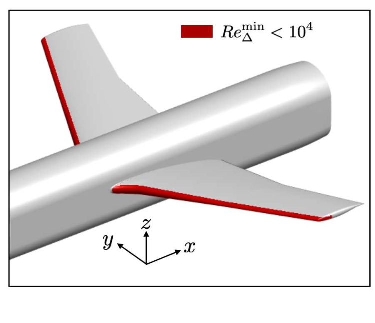
The Reynolds number considered in Figure 3(a) is $Re=5\times 10^{6}$, which is representative of wind tunnel experiments. A Reynolds number typical of aircraft in flight conditions is $Re\approx 5\times 10^{7}$, which would increase $N_{\mathrm{points}}$ by a factor of ten due to the thinning of the boundary layers. More precisely, the increase in $N_{\mathrm{points}}$ is proportional to $Re$ and $N_{bl}$, and roughly inversely proportional to $Re_{\Delta}^{\mathrm{min}}$. The scaling properties of Eq. (4) can be explained by assuming that the boundary layer over the aircraft is fully turbulent and grows as $\delta\sim(x-x_{e})[(x-x_{e})U_{\infty}/\nu]^{-m}$, where $x_{e}$ is the streamwise distance to the closest leading edge and $m\approx-1/7$ for a zero-pressure gradient flat-plate turbulent boundary layer (ZPGTBL). If we further assume that $Re\gg Re_{\Delta}^{\mathrm{min}}$, the number of control volumes can be shown to scale as

$$N_{\mathrm{points}}\sim N_{bl}Re\left(Re_{\Delta}^{\mathrm{min}}\right)^{-5/6},$$

(5)

which is confirmed in Figures 3(c) and (d) using the data obtained using Eq. (4) for the NASA Juncture Flow.

The two isolines in Figure 3(a) bound the region $N_{\mathrm{points}}=100$ million to $1000$ million grid points, which are within the reach of current computing resources available to the industry. For example, for $N_{bl}\approx 10$ and $Re_{\Delta}^{\mathrm{min}}\approx 10^{4}$, the required number of points is $\sim 400$ million, which can be currently simulated in a few days using thousands of cores. However, if the desired accuracy for the quantities of interest is such that $N_{bl}\approx 20$ and $Re_{\Delta}^{\mathrm{min}}\approx 10^{3}$, the number of grid points rises up to $3000$ million, which renders WMLES unfeasible as a routine tool for the industry. Hence, the key to the success of WMLES as a designing tool resides in the accuracy of the solution achieved as a function of $N_{bl}$ and $Re_{\Delta}^{\mathrm{min}}$. This calls for a systematic error characterization of the quantities of interest, which is the objective of the present preliminary work.

We perform WMLES of the NASA Juncture Flow with a leading-edge horn at $Re=2.4\times 10^{6}$ and AoA=$5^{\circ}$. Seven cases are considered. In the first six cases, we use grids generated using strategy (i) with constant grid size in millimeters akin to the example offered in Figure 1(a). In this case, the direct impact of $Re_{\Delta}^{min}$ can be absorbed into $\Delta/\delta$ as is done in Eq. (7). The grid sizes considered are $\Delta\approx 6.7,4.3,2.2,1.1$ and $0.5$ millimeters, which are labeled as C-D7, C-D4, C-D2, C-D1, and C-D0.5, respectively. Cases C-D7, C-D4, and C-D2 are obtained by refining the grid across the entire aircraft surface. For cases C-D1 and C-D0.5, the grid size is, respectively, 1.1 and 0.5 millimeters only within a refinement box along the fuselage and wing-body juncture defined by $x\in[1770,2970]$ mm, $y\in[-300,-200]$ mm, and $z\in[-50,150]$ mm. An additional case is considered to assess the impact on the accuracy of BL-conforming Voronoi grids. The grid is generated using strategy (ii) for $N_{bl}=\delta/\Delta=5$ and $Re_{\Delta}^{\mathrm{min}}=8\times 10^{3}$, as shown in Figure 1(b). The case is denoted as C-N5-Rem8e3.

In the following, $\langle\cdot\rangle$ and $(\cdot)^{\prime}$ denote time-average and fluctuating component, respectively. For comparison purposes, the profiles are interpolated to the grid locations of the experiments. Statistical uncertainties in WMLES quantities are estimated assuming uncorrelated and randomly distributed errors following a normal distribution. The uncertainty in $\langle q\rangle$ is then estimated as $\Delta\langle q\rangle\equiv\sigma/\sqrt{N_{s}}$, where $N_{s}$ is the number of samples for the computing $\langle q\rangle$, and $\sigma$ is the standard deviation of the samples. The uncertainties for the mean velocity profiles and pressure coefficient were found to be below 1% and are not reported in the plots.

We consider three locations on the aircraft: (1) the upstream region of the fuselage, (2) the wing-body juncture, and (3) wing-body juncture close to the trailing edge. The mean velocity profiles are shown in panel (a) of Figures 4, 5, and 6 for each location considered and the errors are quantified in Figure 7(a). We assume that $\langle u_{i}\rangle\approx\langle u_{i}^{\mathrm{exp}}\rangle$ and the mean velocity from WMLES is directly comparable with unfiltered experimental data ($\langle u_{i}^{\mathrm{exp}}\rangle$). The approximation is reasonable for quantities dominated by large-scale contributions, as is the case for $\langle u_{i}\rangle$. Figure 4(a) shows that $\langle u_{i}\rangle$ from WMLES converges to the experimental results with grid refinement. The turbulent boundary layer over the fuselage is about $10$ to $20$ mm thick, which yields roughly 3–6 points per boundary-layer thickness at the grid resolutions considered. Assuming that the flow at a given station can be approximated by a local canonical ZPGTBL, the expected error in the mean velocities can be estimated as $\varepsilon_{m}\approx 0.16\Delta/\delta$ (Lozano-Durán & Bae 2019). For the current $\Delta$, this yields errors of 2%–8%, consistent with the results in Figure 7(a) (red symbols). The situation differs for the wing-body juncture and wing trailing edge. Despite the finer grid sizes, errors in the mean flow prediction are about 15% in the juncture (black symbols in Figure 7a) and even 100% in the trailing edge (blue symbols in Figure 7a). The larger errors may be attributed to the presence of a three-dimensional boundary layers and flow separation in the vicinity of the wing-body juncture and trailing edge, which makes the error scaling predicated upon the assumption of local similarity to a ZPGTBL inappropriate.

The resolved portion of the tangential Reynolds stresses is shown in Figure panels (b) of Figures 4, 5, and 6. The trends followed by $\langle u_{i}^{\prime}u_{j}^{\prime}\rangle$ are correctly captured at the different stations investigated, although their magnitudes tend to be systematically underpredicted, especially for the juncture region and trailing edge. Estimations from Lozano-Durán & Bae 2019 suggest that the error for the turbulence intensities should scale as $\sim(\Delta/\delta)^{2/3}$, which for the present grid resolution implies $\sim 10$–$20\%$ error. The result is consistent with the typical $\Delta$ for WMLES, which supports a limited fraction of the turbulent fluctuations. Assuming $\langle u_{i}^{\mathrm{exp}}\rangle\approx\langle u_{i}\rangle$, then $\langle{u_{i}^{\prime}}^{\mathrm{exp}}{u_{j}^{\prime}}^{\mathrm{exp}}\rangle\approx\langle u_{i}^{\prime}u_{j}^{\prime}\rangle+\langle\tau_{ij}^{\mathrm{SGS}}\rangle$, where $\tau_{ij}^{\mathrm{SGS}}$ is the subgrid-scale tensor. Thus, for the current grid sizes we can expect $|\langle u_{i}^{\prime}u_{j}^{\prime}\rangle|<|\langle{u_{i}^{\prime}}^{\mathrm{exp}}{u_{j}^{\prime}}^{\mathrm{exp}}\rangle|$, i.e., severe underprediction of the tangential Reynolds stress by WMLES.

Figure 7(a) is the cornerstone of the present study. It shows the relative errors in the prediction of the mean velocity profiles for the three regions considered: upstream fuselage, wing-body juncture, and wing-body juncture at the trailing edge. The three regions are marked with lines in Figure 7(b) using the same colors as in Figure 7(a). The turbulent flow in the fuselage resembles a ZPGTBL. As such, the wall- and SGS models, which have been devised for and validated in flat-plate turbulence, perform accordingly. On the contrary, there is a clear decline of current models in the wing-body juncture and trailing edge region, which are dominated by secondary motions in the corner and flow separation. Not only is the magnitude of the errors larger in the latter locations, but the error rate of convergence is also slower ($\varepsilon_{m}\sim(\Delta/\delta)^{0.5}$) when compared with the equilibrium conditions encountered in ZPGTBL ($\varepsilon_{m}\sim(\Delta/\delta)$). The situation could be even more unfavorable, as Lozano-Durán & Bae 2019 has shown that for refining grid resolutions the convergence of WMLES towards the DNS solution may follow a non-monotonic behavior due to the interplay between numerical and SGS model errors.

The surface pressure coefficient over the wing, $C_{p}$, is shown in Figure 8 along the chord of the wing. The predictions are compared with experimental data at three different $y$-locations. The locations selected are denoted by red lines in Figure 8(d). Overall, WMLES agrees with the experimental data to within 1–5% error. The predictions are still to within 5% accuracy even at the coarsest grid resolutions considered, which barely resolved the boundary layer. The main discrepancies with experiments are located at the leading edge of the wing.

The accurate prediction of $C_{p}$ is a common observation in CFD of external aerodynamics. The result can be attributed to the outer-layer nature of the mean pressure, which becomes less sensitive to the details of near-wall turbulence. Under the thin boundary-layer assumption, the integrated mean momentum equation in the spanwise direction shows that $\langle p\rangle+\rho\langle v^{2}\rangle\approx p_{e}(x)\Rightarrow p_{\mathrm{wall}}=p_{e}(x)$, where $p_{e}$ is the far-field pressure. Hence, the pressure at the surface is mostly imposed by the inviscid imprint of the outer flow. This is demonstrated by performing an additional calculation similar to C-D2 but imposing the free-slip boundary condition at the wall such that boundary layers are unable to develop (Figure 8(c)). The conditions for $p_{\mathrm{wall}}=p_{e}(x)$ would not hold, for example, when the wall radius of curvature is comparable to the boundary-layer thickness. This is the case in the vicinity of the wing leading-edge, which is the region where the accuracy of $C_{p}$ provided for WMLES is the poorest and most sensitive to $\Delta$. The tripping methodology used in WMLES differs from the experimental setup, which may also contribute to the discrepancies observed.

The outer-flow character of $C_{p}$ is encouraging for the prediction of the pressure-induced components of the lift and drag coefficients. It also suggests that $C_{p}$ might not be a challenging quantity to predict in the presence of wall-attached boundary layers. Thus, the community should focus the efforts on other important quantities of interest such as the numerical prediction of the skin-friction coefficient and its challenging experimental measurement.

For completeness, we also report the results on the size of the separation bubble. The mean wall-stress streamlines for case C-D0.5 are shown in Figure 9. The figure also contains a depiction of the average length and width of the separation bubble, which are about $100$ mm and $60$ mm, respectively, for case C-D0.5. Direct comparison of these dimensions with oil-film experimental results show that the current WMLES prediction is about 15% lower than the experimental measurements ($120\times 80$ mm), consistent with previous WMLES investigations (Lozano-Durán et al. 2020; Iyer & Malik 2020; Ghate et al. 2020). Nonetheless, note that the sizes of the separation zone from WMLES are obtained from the tangential wall-stress streamlines after the wall stress is averaged in time, whereas the experimental sizes are obtained from the pattern resulting from the oil-film time evolution. Albeit both methodologies provide an average description of the size of the separation zone, they do not allow for a one to one comparison and we should not interpret the present differences as a faithful quantification of the errors. Hence, a methodology allowing for quantitative comparisons of separated-flow patterns between CFD and experimental data remains an open challenge.

We evaluate potential improvements with BL-conforming grids by comparing the results for case C-N5-Rem8e3 with case C-D2. The grid for C-N5-Rem8e3 is generated for $N_{bl}=5$ and $Re_{\Delta}^{\mathrm{min}}=10^{4}$ following the procedure described in Section 3.1. For reference, case C-D2 has 32 million control volumes, whereas case C-N5-Rem8e3 has 11 million control volumes. The mean velocity profiles for C-N5-Rem8e3 are shown in Figure 10 and compared with C-D2 at three locations. Some moderate improvements are achieved at the fuselage despite both cases sharing the same $N_{bl}$ at that location. The improvements are accentuated at the juncture and trailing edge, where C-N5-Rem8e3 outperforms C-D2 with less than a fourth of the grid points per $\delta$ in each of the three spatial directions.

The results suggest that grids designed to specifically target the boundary layer could improve the overall accuracy of WMLES. The outcome might be explained by considering the upstream history of the WMLES solution at a given station. Let’s assume the simpler scenario of WMLES of a flat-plate turbulent boundary layer along $x$ using two grids: a constant-size grid and a BL-conforming grid. If we take an $x$-location at which both grids have the same $N_{bl}$, the upstream flow for the constant-size grid is underresolved compared to the BL-conforming grid due to the thinner $\delta$ upstream the flow (hence, less points per $\delta$ and larger errors). On the other hand, the BL-conforming grid maintains a constant grid resolution scaled in $\delta$ units and effectively more resolution upstream the flow. Furthermore, even if at a given $x$ location $N_{bl}$ is larger for the constant-size grid, the solution could be worse because of error propagation from the upstream flow. By assuming that energy-containing eddies with lifetimes $\delta/U_{\infty}$ are advected by $U_{\infty}$, we can estimate the downstream propagation of errors at a given location $x_{0}$ by $\Delta x_{e}=\int_{x_{0}}^{x}\delta_{0}/\delta\,\mathrm{d}x$, which is the streamwise distance required for the energy-containing eddies to forget their past history. In ZPGTBL at high $Re$ (Sillero et al. 2013), $\Delta x_{e}$ can reach values of $\Delta x_{e}\approx 100\delta_{0}$. The long convective distance for error propagation ($\sim 200$ mm for $\delta_{0}\approx\Delta=2$ mm) combined with the higher upstream errors for constant-size grids may explain the improved results for C-N5-Rem8e3 reported in Figure 10.

References

- Bose & Park (2018) Bose, S. T. & Park, G. I. 2018 Wall-modeled large-eddy simulation for complex turbulent flows. Annu. Rev. Fluid Mech. 50, 535–561.
- Chapman (1979) Chapman, D. R. 1979 Computational aerodynamics development and outlook. AIAA J. 17, 1293–1313.
- Choi & Moin (2012) Choi, H. & Moin, P. 2012 Grid-point requirements for large eddy simulation: Chapman’s estimates revisited. Phys. Fluids 24, 011702.
- Clark et al. (2020) Clark, A. M., Slotnick, J. P., Taylor, N. J. & Rumsey, C. L. 2020 Requirements and challenges for CFD validation within the High-Lift Common Research Model ecosystem. AIAA Paper 2020-2772.
- Germano et al. (1991) Germano, M., Piomelli, U., Moin, P. & Cabot, W. H. 1991 A dynamic subgrid-scale eddy viscosity model. Phys. Fluids 3, 1760.
- Ghate et al. (2020) Ghate, A. S., Housman, J. A., Stich, G.-D., Kenway, G. & Kiris, C. C. 2020 Scale Resolving Simulations of the NASA Juncture Flow Model using the LAVA Solver. AIAA Paper 2020-2735.
- Iyer & Malik (2020) Iyer, P. S. & Malik, M. R. 2020 Wall-modeled LES of the NASA Juncture Flow Experiment. AIAA Paper 2020-1307.
- Kawai & Larsson (2012) Kawai, S. & Larsson, J. 2012 Wall-modeling in large eddy simulation: Length scales, grid resolution, and accuracy. Phys. Fluids 24, 015105.
- Kegerise et al. (2019) Kegerise, M. A., Neuhart, D., Hannon, J. & Rumsey, C. L. 2019 An experimental investigation of a wing-fuselage junction model in the NASA Langley 14- by 22-foot subsonic wind tunnel. AIAA Paper 2019-0077.
- Larsson et al. (2016) Larsson, J., Kawai, S., Bodart, J. & Bermejo-Moreno, I. 2016 Large eddy simulation with modeled wall-stress: recent progress and future directions. Mech. Eng. Rev. 3, 1–23.
- Lee et al. (2018) Lee, H., Pulliam, T., Rumsey, C. & Carlson, J.-R. 2018 Simulations of the NASA Langley 14-by 22-Foot Subsonic Tunnel for the Juncture Flow Experiment. In NATO STO.
- Lee & Pulliam (2019) Lee, H. C. & Pulliam, T. H. 2019 Overflow juncture flow computations compared with experimental data. AIAA Paper 2019-0080.
- Lee et al. (2017) Lee, H. C., Pulliam, T. H., Neuhart, D. & Kegerise, M. A. 2017 CFD analysis in advance of the NASA Juncture Flow Experiment. AIAA Paper 2017-4127.
- Lilly (1992) Lilly, D. K. 1992 A proposed modification of the Germano subgrid-scale closure method. Phys. Fluids 4, 633–635.
- Lozano-Durán & Bae (2019) Lozano-Durán, A. & Bae, H. J. 2019 Error scaling of large-eddy simulation in the outer region of wall-bounded turbulence. J. Comput. Phys. 392, 532–555.
- Lozano-Durán & Bae (2020) Lozano-Durán, A. & Bae, H. J. 2020 Self-critical machine-learning wall-modeled LES for external aerodynamics. Center for Turbulence Research - Annual Research Briefs pp. XX–XX.
- Lozano-Durán et al. (2020) Lozano-Durán, A., Bose, S. T. & Moin, P. 2020 Prediction of trailing edge separation on the NASA Juncture Flow using wall-modeled LES. AIAA Paper 2020-1776.
- Poinsot & Lele (1992) Poinsot, T. & Lele, S. 1992 Boundary conditions for direct simulations of compressible viscous flows. J. Comput. Phys. 101, 104–129.
- Rumsey (2018) Rumsey, C. L. 2018 The NASA Juncture Flow Test as a model for effective CFD/experimental collaboration. AIAA Paper 2018-3319.
- Rumsey et al. (2019) Rumsey, C. L., Carlson, J. & Ahmad, N. 2019 FUN3D Juncture Flow computations compared with experimental data. AIAA Paper 2019-0079.
- Rumsey & Morrison (2016) Rumsey, C. L. & Morrison, J. H. 2016 Goals and status of the NASA Juncture Flow Experiment. In NATO STO.
- Rumsey et al. (2016) Rumsey, C. L., Neuhart, D. & Kegerise, M. A. 2016 The NASA Juncture Flow Experiment: goals, progress, and preliminary testing (Invited). AIAA Paper 2016-1557.
- Sillero et al. (2013) Sillero, J. A., Jiménez, J. & Moser, R. D. 2013 One-point statistics for turbulent wall-bounded flows at Reynolds numbers up to . Phys. Fluids 25, 105102.
- Slotnick et al. (2014) Slotnick, J., Khodadoust, A., Alonso, J., Darmofal, D., Gropp, W., Lurie, E. & Mavriplis, D. 2014 CFD Vision 2030 Study: A Path to Revolutionary Computational Aerosciences.
- Spalart (2009) Spalart, P. R. 2009 Detached-eddy simulation. Annu. Rev. Fluid Mech. 41, 181–202.
- Spalart et al. (1997) Spalart, P. R., Jou, W. H., Strelets, M., Allmaras, S. R. et al. 1997 Comments on the feasibility of LES for wings, and on a hybrid RANS/LES approach. Advances in DNS/LES, 4–8.
- Vassberg et al. (2008) Vassberg, J. C., Tinoco, E. N., Mani, M., Brodersen, O. P., Eisfeld, B., Wahls, R. A., Morrison, J. H., Zickuhr, T., Laflin, K. R. & Mavriplis, D. J. 2008 Abridged summary of the third AIAA computational fluid dynamics drag prediction workshop. J. Aircr. 45, 781–798.
- Wang & Moin (2002) Wang, M. & Moin, P. 2002 Dynamic wall modeling for large-eddy simulation of complex turbulent flows. Phys. Fluids 14, 2043–2051.