Locally conservative immersed finite element method for elliptic interface problems

In this section, we review and discuss the classical immersed finite element method to handle the problem (2.19). Let $\mathcal{T}_{h}$ be a regular triangulation of $\Omega$. We note that the triangulation is provided in general for which nodes are not necessarily aligned with the interface $\Gamma$. Under this setting, there are two types of triangles in $\mathcal{T}_{h}$, i.e., an interface element $T$, which is characterized by the fact that it is cut by the interface $\Gamma$ and a non-interface element $T$ which is not. We shall denote $\mathcal{T}_{h,\Gamma}\subset\mathcal{T}_{h}$, by the set of interface triangles. We shall let $\mathcal{E}_{h}$ be the set of edges of $\mathcal{T}_{h}$. Note that $\mathcal{E}_{h}=\mathcal{E}_{h}^{o}\cup\mathcal{E}_{h}^{\partial}$, where $\mathcal{E}_{h}^{o}$ is the set of interior edges while $\mathcal{E}_{h}^{\partial}$ is the set of boundary edges.

The space $H^{s}(\mathcal{T}_{h})(s\in{\rm I\!R})$ is the set of element-wise $H^{2}$ functions on $\mathcal{T}_{h}$, and $L^{2}(\mathcal{T}_{h})$ refers to the set of element-wise $L^{2}$ functions. Following arnold2002unified, for any $e\in\mathcal{E}_{h}$, we denote by $|e|$ the length of the edges $e$. Now let $e\in\mathcal{E}_{h}^{o}$, $T^{+}$ and $T^{-}$ denote two neighboring elements such that $e=\partial T^{+}\cap\partial T^{-}$. Let $\mathbf{n}^{+}$ and $\mathbf{n}^{-}$ be the outward normal unit vectors to $\partial T^{+}$ and $\partial T^{-}$, respectively. For any given function $\xi$ and vector function ${\xi}$ $\scriptscriptstyle\bf{\sim}$ , defined on the triangulation $\mathcal{T}_{h}$, we denote $\xi^{\pm}$ and ${\bf{\xi}}^{\pm}$ by the restrictions of $\xi$ and ${\bf{\xi}}$ to $T^{\pm}$, respectively. We define the average $\{\!\!\{\cdot\}\!\!\}$ as follows: for $\zeta\in L^{2}(\mathcal{T}_{h})$ and $\hbox{\vtop{\halign{#\cr${\tau}$\crcr$\scriptscriptstyle\bf{\sim}$\crcr}}}\in L^{2}(\mathcal{T}_{h})^{d}$,

On the other hand, for $e\in\mathcal{E}_{h}^{\partial}$, we set $\{\!\!\{\zeta\}\!\!\}:=\zeta$ and $\{\!\!\{\hbox{\vtop{\halign{#\cr${\tau}$\crcr$\scriptscriptstyle\bf{\sim}$\crcr}}}\}\!\!\}:=\hbox{\vtop{\halign{#\cr${\tau}$\crcr$\scriptscriptstyle\bf{\sim}$\crcr}}}$. The jump across the interior edge will be defined as usual:

For $e\in\mathcal{E}_{h}^{\partial}$, we set $[\![\zeta]\!]=\zeta\mathbf{n}$. For any given edge $e\in\mathcal{E}_{h}^{o}$, there are two choices of the normal $\mathbf{n}$ to $e$ and it is useful to fix one of them, for example, for an appropriate definition of the flux. Such a fixed choice of the normal to $e$ will be denoted by $\mathbf{n}_{e}.$

For any $T\in\mathcal{T}_{h}$ and an inner product $(\cdot,\cdot)_{m,T}$, the computation can be done with the following decomposition:

We will let $\mathcal{P}^{k}(T)$ denote the space of polynomials of degrees less than or equal to $k$ for a given $T\in\mathcal{T}_{h}$. Similarly, we also let $\mathcal{P}^{k}(e)$ denote the space of polynomials of degree less than or equal to $k$ for a given $e\in\mathcal{E}_{h}$.

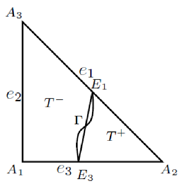
Given a non-interface element $T$, we shall recall that $S_{h}(T)=\mathcal{P}^{1}(T)={\rm span}\{\lambda_{j}\}_{j=1,2,3}$, where $\lambda_{j}$’s are standard barycentric coordinates, i.e., $\lambda_{j}(A_{i})=\delta_{ij}$, where $A_{i}$’s are nodes of $T$ and $\delta_{ij}$ is the standard Kronecker delta function. In case $T$ is an interface element, the space $S_{h}(T)$ will be modified as $\widehat{S}_{h}(T)={\rm span}\{\widehat{\lambda}_{j}\}_{j=1,2,3}$, so that $\widehat{\lambda}_{j}$ satisfies the interface condition as well as $\widehat{\lambda}_{j}(A_{i})=\delta_{ij}$. More precisely, as described in Figure 2, given an interface element $T$, we suppose the interface $\Gamma$ cuts $T$ through edges $e_{1}$ and $e_{3}$ of $T$ at points $E_{2}$ and $E_{1}$. This cut will divide $T$ into $T^{+}$ contained in $\Omega^{+}$ and $T^{-}$ contained in $\Omega^{-}$.

For $j=1,2,3$, we modify $\lambda_{j}\in S_{h}(T)$ to a piecewise linear function $\widehat{\lambda}_{j}$ of the following form:

where the coefficients $\{a_{j}^{\pm},b_{j}^{\pm},c_{j}^{\pm}\}$ are determined by the jump conditions and vertex degrees of freedom:

It is well known that the aforementioned conditions (2.13) uniquely determine $\widehat{\lambda}_{j}$ for $j=1,2,3$, (see chou2010optimal). The vertex based piecewise linear immersed finite element space (IFEM) for the problem (2.19) is then characterized by the space $\widehat{S}_{h}(\Omega)$ defined as follows: for $\phi\in\widehat{S}_{h}(\Omega)$, it holds

The approximation property of the space $\widehat{S}_{h}(\Omega)$ is well known, he2008approximation; kwak2010analysis; li2004immersed. Namely, let $\ell_{h}:H^{2}(T)\to\widehat{S}_{h}(T)$ be the standard local nodal interpolation operator defined by, for $v\in H^{2}(T)$,

We then let $I_{h}:\widetilde{H}^{2}(\Omega)\to\widehat{S}_{h}(\Omega)$ be the extension of $\ell_{h}$ defined by $I_{h}(v)|_{T}=\ell_{h}(v|_{T})$. The following has been established:

The classic IFEM construct a finite element solution to the problem (2.19), by solving the following discrete weak formulation: find $p_{h}\in\widehat{S}_{h}(\Omega)$ such that

Recently, it is observed that the partially penalized IFEM is of optimal convergence in the energy norm Lin2015partially, which will be adopted in our paper (see Section 3 for detailed description). To clarify the proposed conservative IFEM formulation, we state the definition of local and global conservation.

We would like to remark that the conservation is dependent on the choice of triangulations, $\mathcal{T}_{h}$. The issue with the conservation has drawn a lot of attention in literatures (see sun2009locally; lee2015locally and references cited therein). Due to the absence of the piecewise constant in the IFEM space, the standard and its variant IFEMs are not locally or globally conservative.

We enrich the standard IFEM space $\widehat{S}(\Omega)$ by piecewise constant functions. The idea has been introduced at sun2009locally; lee2015locally. However, both of works are limited to the case when the mesh fits in the interface. This is the first attempt to introduce the enrichment for the interface problem where the interface is not necessarily aligned with the mesh. We shall denote by $E_{h}$, the enriched IFEM space, i.e., we define

where

To clarify the EIFEM formulation, we shall set the fixed unit normal vector for any given edge $e\in\mathcal{E}_{h}$, which will be denoted by ${\bf{n}}$. Note that the dimension of the space $\widehat{S}_{h}(\Omega)$ is the number of interior nodes for the triangulation $\mathcal{T}_{h}$, which will be denoted by $N_{0}$ while the dimension of the space $C_{h}$ is the number of elements, which will be denoted by $N_{e}$. We first, consider the space $H_{h}(\Omega):=\widetilde{H}^{1}(\Omega)+E_{h}(\Omega)$ and equip it with a broken $H^{1}$-norm:

We introduce the scalar $L^{2}$ projection, $Q_{e}^{0}:H^{1/2}(e)\mapsto\mathcal{P}^{0}(e)$ and the vector $L^{2}$ projection, ${\bf{Q}}_{e}^{0}:(H^{1/2}(e))^{2}\mapsto(\mathcal{P}^{0}(e))^{2}$, defined, respectively by

We note that $Q_{h}^{0}:L^{2}(\Omega)\mapsto C_{h}$ denotes the standard $L^{2}$ projection onto $C_{h}$. In this section, we shall establish the optimal approximation property for EIFEM, both in the primal and flux variables. We begin with the EIFEM interpolation. Motivated by Lee et. al lee2015locally, we introduce the EIFEM-interpolation operator $\Pi_{h}:\widetilde{H}^{2}(\Omega)\mapsto E_{h}$ as follows:

We define the bilinear form $a_{h}(\cdot,\cdot):H_{h}(\Omega)\times H_{h}(\Omega)\mapsto{\rm I\!R}$ by, for all $v,w\in H_{h}(\Omega)$,

where $|e|$ is the measure of $e$, the symbol $\theta$ will be discussed below, and the symbol $\sigma(\beta)$ is to indicate that $\sigma$, the stabilization parameter is chosen depending on $\beta$ in each edge $e\in\mathcal{E}_{h}$. Theoretically, at the interface edge, $\sigma=\kappa\overline{\beta}/\underline{\beta}$ for some $\kappa>0$ gives sufficient stabilization.

We are now in a position to state the enriched immersed finite element to solve (2.5). The enriched IFEM can then be formulated as follows: find $p_{h}\in E_{h}$ such that

The bilinear form, here is the one that corresponds to interior penalty DG method, introduced in wheeler1978elliptic. The symbol $\theta$ is the tuning parameter, which determines the type of interior penalty method, i.e., $\theta=-1,0$ and $1$ result in NIPG, IIPG and SIPG, respectively sun2009locally; lee2015locally.

We shall now list couple of simple but important observations for the problem (3.7). We begin with the consistency.

For the coercivity of the bilinear form $a_{h}(\cdot,\cdot)$, we state and prove a simple, but important lemma:

We are in a position to establish the coercivity of the bilinear form $a_{h}(\cdot,\cdot)$.

The continuity of the bilinear form $a_{h}(\cdot,\cdot)$ can be proven by the same techniques used in the proof of Lemma 5.

We now state and prove the error estimate for the primary variable in $|\!|\!|\cdot|\!|\!|_{h}$-norm.

Finally, we state the error estimate in $L^{2}$-norm.