Particle Swarm Based Hyper-Parameter Optimization for Machine Learned Interatomic Potentials
Abstract
Modeling non-empirical and highly flexible interatomic potential energy surfaces (PES) using machine learning (ML) approaches is becoming popular in molecular and materials research. Training an ML-PES is typically performed in two stages: feature extraction and structure-property relationship modeling. The feature extraction stage transforms atomic positions into a symmetry-invariant mathematical representation. This representation can be fine tuned by adjusting on a set of so-called “hyper-parameters” (HPs). Subsequently, an ML algorithm such as neural networks or Gaussian process regression (GPR) is used to model the structure-PES relationship based on another set of HPs. Choosing optimal values for the two sets of HPs is critical to ensure the high quality of the resulting ML-PES model.
In this paper, we explore HP optimization strategies tailored for ML-PES generation using a custom-coded parallel particle swarm optimizer (available freely at https://github.com/suresh0807/PPSO.git). We employ the smooth overlap of atomic positions (SOAP) descriptor in combination with GPR-based Gaussian approximation potentials (GAP) and optimize HPs for four distinct systems: a toy C dimer, amorphous carbon, -Fe and small organic molecules (QM9 dataset). We propose a two-step optimization strategy in which the HPs related to the feature extraction stage are optimized first, followed by the optimization of the HPs in the training stage. This strategy is computationally more efficient than optimizing all HPs at the same time by means of significantly reducing the number of ML models needed to be trained to obtain the optimal HPs. This approach can be trivially extended to other combinations of descriptor and ML algorithm, and brings us another step closer to fully automated ML-PES generation.
keywords
hyper-parameter optimization, machine learning, interatomic potentials, potential energy surfaces1 Introduction
Studying the dynamic motion of atoms in molecular and material systems with femtosecond resolution is made possible via molecular dynamics (MD) simulations. Allen and Tildesley 2017 In the last few decades our reliance on such simulations to understand complex systems has increased steadily, driven by advances in computer architectures and the availability of more accurate mathematical functions describing interatomic interactions. Hollingsworth and Dror 2018 Numerical integration of Newton’s equations of motion, one time step at a time, to sample the phase space of the model system, requires access to the forces acting on the atoms in the system, i.e., the negative gradient of the potential energy surface (PES). Historically, these forces are obtained from empirical potentials (“force fields”) that incorporate physically inspired functional forms fitted to experimental and/or ab initio reference data. This type of simulation is termed classical molecular dynamics (CMD). MacKerell Jr 2004 As computer power increased, it became possible to compute accurate forces on-the-fly from the electronic structure of the atomic system at every time step, termed ab initio molecular dynamics (AIMD). Marx and Hutter 2009 There is an inescapable trade off between accuracy and flexibility, on the one hand, and computational cost, on the other, to simulate atomic systems. Thus, there is a great drive to develop new methods that are as fast as CMD and as accurate as AIMD. This is where PES learned by machine learning algorithms (MLAs) present themselves as an optimal solution. Handley and Popelier 2010; Behler 2016; Schmitz et al. 2019; Mueller et al. 2020; Dral et al. 2020; Deringer et al. 2019
MLAs enable us to understand, find patterns in and predict future outcomes of complex systems from huge volumes of data accumulated from both experiments and simulation. Liu et al. 2010; Butler et al. 2013; Fenton et al. 2018; de Pablo et al. 2019; Schmidt et al. 2019; Meredig 2019; Morgan and Jacobs 2020 Establishing a strong structure-property relationship is at the core of the ML strategy in developing applications for chemical systems. These ML models rely on a number of so-called hyper-parameters (HPs) affecting their performance. These HPs control the learning rate (how much data is needed to achieve a certain accuracy) and the interpolation power (what accuracy can the ML model achieve with a given data set). Therefore, HP optimization is a critical step towards ensuring that a given ML model is making the most out of the available data, and an integral part in the training workflow, which for ML-PES models can be summarized as follows:
- 1.
Building a reference database of atomic positions and corresponding properties (energies, forces, etc.)
- 2.
Symmetry-invariant feature extraction from atomic positions
- 3.
Hyper-parameter optimization
- 4.
Training and validating the ML model
Building a reference database includes careful selection of reference structures representing the material/chemical system and a reference method to compute their properties. The reference method is usually more expensive to evaluate than the ML model. A reference method that is commonly used to describe condensed-phase systems with reasonable accuracy and felxibility is Kohn-Sham density functional theory (DFT). Kohn and Sham 1965 However, researchers have also used more accurate (and relatively more expensive) wave function based methods as reference to train ML models of molecular systems. Schran et al. 2018; Chmiela et al. 2018
To validate the trained ML model, a test set must be created. This could simply be a fraction of the reference database (“train/test split”) or could involve a complex suite of test simulations (stiffness tensor, phonon spectra, phase diagrams, etc.). Usually, the former is a good choice in the preliminary stages, whereas the most promising ML models could be further scrutinized using the latter.
Since the atomic positions of a reference structure are not invariant with respect to rotation and translation of atoms, they are unsuitable to be used directly as input for training the ML model. Therefore, positions must first be converted to an invariant representation. This representation could encode the entire structure, termed as ‘global descriptor’, such as Coulomb matrix Rupp et al. 2012 and many body tensor representation, Huo and Rupp 2017 or every atom in the system individually, termed as ‘local descriptor’. Himanen et al. 2020 For training ML-PES of condensed-phase systems, local descriptors are desirable and the total energy of the system can be computed as a sum of atom-wise energy contributions. Christensen et al. 2020 This also allows for transferability of the ML-PES. There are several descriptor commonly used in the representation of atomic structures. Himanen et al. 2020 Two of the most widely used approaches are the smooth overlap of atomic positions (SOAP) Bartók et al. 2013; Caro 2019 and atom-centered symmetry functions (ACSF). Behler 2011 These approaches encode the immediate chemical environment of every atom in the system into a set of invariants (simply ‘descriptors’, from here onward), which form the training data along with the properties obtained from the reference method. It has been shown that these representations are formally related to one another Willatt et al. 2019. Imbalzano et al. Imbalzano et al. 2018 have previously identified efficient methods to automatically optimize the size of ACSF and SOAP fingerprints to describe the atomic environment of the desired chemical system. We also note there exist neural networks that use deep learning to extract the symmetry invariants directly from the input 3D structural data. Schütt et al. 2017 For ML-PES training, the reference properties typically include the total energy of the structure, atomic force components, virial stress components and atomic charges.
The ML algorithm is responsible for establishing the structure-property relationship. The two most popular ML algorithms for condensed-phase ML-PES training are Behler-Parrinello type neural networks (BPNN) Behler and Parrinello 2007 and Gaussian process regression (GPR, generally known in the community as Gaussian approximation potential, GAP). Bartók et al. 2010; Bartók and Csányi 2015 GPR is a particular flavor of the more general class of kernel-based regression algorithms Christensen et al. 2020. Both ML and descriptor algorithms have adjustable HPs, that need to be optimized for the target system. Since training an ML model is an expensive endeavor in terms of computational time, rigorous HP optimization (HPO) is often impractical due to the large HP search space. For the same reason, the HPs in the earlier ML-PES models have been selected either from chemical intuition Bernstein et al. 2019, grid search, stochastic search, Christensen et al. 2020 or from testing a small number of HP combinations using approaches similar to the design of experiments. More recently, we performed a Sobol sequence based HP search to obtain optimal HPs for an amorphous carbon GAP.Caro 2019 Schmitz et al. Schmitz et al. 2019 performed HP optimization of a GPR model of the molecule using open source optimizers. Recently, an application to automate molecular PES training using the HyperOpt Bergstra et al. 2015 optimizer has been introduced. Abbott et al. 2019 It is important to note that an accurate model of the whole HP surface is not needed because we are only interested in its global minimum.
While there are deterministic algorithms that are guaranteed to find the global minimum of high dimensional functions, they are impractical for finding solutions to multi-parameter dependent real world problems, which are in most cases NP-hard. By contrast, heuristics-based stochastic algorithms, although not guaranteed to find the global minimum in every instance, have the best chance to find solutions to such problems. Collet and Rennard 2008 There are several non-traditional HPO techniques for ML models available in the literature such as Bayesian optimization, random forest algorithm and particle swarm optimization Bergstra et al. 2015; Feurer and Hutter 2019. However, we are unaware of any HPO strategy tailored specifically for complex ML-PES training. A specialized strategy is necessary since the impact of each hyper-parameter on the accuracy and performance of the ML-PES model is not the same. While good values for hyper-parameters can be guessed for simple and well studied chemical systems, guessing them is impossible for new and complex systems. In this paper, we look at optimization strategies specific to the HPs encountered in ML-PES training using a custom coded parallel particle swarm optimizer, which is a heuristic based stochastic optimizer. We will consider the combination of SOAP descriptors and GAP ML model in this paper, but it is possible to trivially extend the discussed strategies to other descriptors and ML schemes as well. Incorporating these strategies into the training workflow will bring us one step closer to efficient fully automated ML-PES generation.
2 Hyper-Parameter Classification
Figure 1 shows an overview of the steps involved in a ML-PES training workflow. There are two important stages, the feature extraction (FE) stage and the machine learning algorithm (MLA) stage, in which two distinct sets of HPs are needed. The FE stage converts the atomic coordinates in the reference database into descriptors . This transformation depends parametrically on a set of HPs, {HP}FE. The MLA stage relates the descriptors to the corresponding quantum chemical reference data ( and ), based on another set of HPs, {HP}MLA.

In the FE stage, {HP}FE controls how the representation of the atoms is carried out. For many-body descriptors, such as SOAP and ACSFs, this representation may involve the assignment of each atomic position to an atomic density, as well as the construction of a basis set for finite numerical expansion of this atomic density. This is conceptually very similar to how electron densities are represented in DFT codes (e.g., by using localized atomic orbitals). The symmetry-invariant representation of into leads to a mapping from an dimensional space to an dimensional space, where is the number of atoms and is the dimension of each atomic descriptor . This generally leads to a significant increase in dimensionality, since usually . The {HP}FE can be further split into two subsets, {HP} and {HP}, where {HP} controls the size () of the descriptor and the computational effort needed, via adjusting the number of basis functions, while {HP} affects the shape of the atomic density representation (i.e., how a point atom is “smeared” into a density field). An optimal {HP}FE is desirable, such that the resulting descriptors are not only optimally sized so that they will not be too expensive to compute but also maximally detailed so as to better differentiate between atomic environments.
In the MLA stage, the quality of the structure-property relationship depends on the choice of {HP}MLA along with the choice of {HP}FE in the FE stage. Similar to the FE stage, {HP}MLA can also be split into two subsets {HP} and {HP}. For example, in artificial neural networks, a HP could be the number of hidden layer neurons in the network while a HP could be the choice of activation function in the hidden layer neurons (e.g., using a sigmoid function instead of a hyperbolic tangent does not increase the computational cost but only changes the output value range). The total number of HPs combining those from FE and MLA stages, , can be small or large depending on the choice of the descriptor and MLA. Each point in this dimensional space has a ML-PES and a quality estimate associated to it. As mentioned earlier, our aim is not to model this dimensional objective function but to find its global minimum as cheaply and efficiently as possible. For the remainder of this paper we will use SOAP in the FE stage and GAP in the MLA stage.
3 SOAP, GAP and Objective Functions
Let us first look at how SOAP and GAP allow us to predict energies and forces in a simple practical way. For more extensive details please refer to the literature. Bartók et al. 2010; Bartók et al. 2013; Bartók and Csányi 2015; Caro 2019 Let us consider a training database containing structures each with atoms (or, equivalently, atomic environments). First, the bits of Cartesian positions information () of the reference database are transformed into bits of information () based on the choice of {HP}SOAP:
| (1) |
using the SOAP formalism introduced by Bartók et al. Bartók et al. 2013 Here, we work with the SOAP-type descriptors introduced by us elsewhere, Caro 2019 to which we refer as soap_turbo.
Every atomic environment is bounded by a SOAP cutoff sphere (CS) with radius . The atomic density of the environment of atom is approximated by an expansion in radial basis and spherical harmonics : Bartók et al. 2013
| (2) |
Here, and are the indices for radial and angular channels, respectively. The maximum values of and control the size of the basis. takes the integer values between and . The outer sum is over all the atoms, , that are within the cutoff sphere of (CSi), and the are the expansion coefficients. The components of the SOAP descriptor for atomic environment are obtained from the normalized power spectrum of the corresponding atomic density:
| (3) |
The total number of invariant components describing the atomic environment, with elemental species in it, is given by
| (4) |
where and are the total number of radial and angular momentum channels used in the basis set, respectively (the division by 2 is for the symmetry of the coefficients upon exchange of the radial basis indices; Caro 2019 next to is to include ). To get an idea of the typical dimensionality of SOAP descriptors, consider the following example: if we choose and , we end up with 605 SOAP components for a single species descriptor (). This value increases to 2310 components for . Therefore, computing SOAP descriptors becomes increasingly more expensive as the atomic environment becomes more heterogeneous (“curse of dimensionality”). Hence, and are critical performance-based HPs. Another HP that significantly affects the performance is , which determines the total number of neighbor atoms to be considered inside the SOAP sphere for the many-body descriptor evaluation (the cost of building SOAP descriptors and descriptor gradients grows as ). Brief descriptions of all {HP}SOAP+GAP are given in Table 1. From Table 1, there are 11 soap_turbo HPs in total out of which 3 are performance affecting HPs and the other 8 are shape affecting HPs. Except , all the other HPs can be given as a vector of components. Choosing different values for each species increases the total number of unique SOAP HPs to . We also note that this is the maximum number of HPs to be optimized; one can choose to constrain the search to those HPs that are expected to have the biggest impact on model accuracy, and set the rest to the default values.
| HP | Symbol | Units | Description |
|---|---|---|---|
| {HP} | |||
| number of radial channels | |||
| number of angular momentum channels | |||
| rcut_hard | rch | Å | cutoff radius for SOAP sphere |
| {HP} | |||
| rcut_soft | rcs | Å | density smoothing enabled beyond this value |
| atom_sigma_r | Å | width of Gaussian functions in radial channels | |
| atom_sigma_t | Å | width of Gaussian functions in angular channels | |
| atom_sigma_r_scaling | ar | radial dependence of functions in radial channels | |
| atom_sigma_t_scaling | at | radial dependence of functions in angular channels | |
| amplitude_scaling | a | radial dependence of neighbour contribution | |
| central_weight | cw | Gaussian width for the central atom | |
| radial_enhancement | re | factor to enhance the amplitude of radial Gaussians | |
| zeta | SOAP kernel is raised to the power of | ||
| {HP} | |||
| n_sparse | number of sparse configuration to be used | ||
| {HP} | |||
| delta | eV | energy contribution scaling factor | |
| sigma_E | eV | regularization parameter for energies | |
| sigma_F | eV/Å | regularization parameter for forces | |
In the next step, a GAP is generated by Gaussian process regression (GPR) from the reference energies and forces, where the covariance between two atomic energies and is obtained from the SOAP-based kernel (which measures the similarity between atomic environments and ):
| (5) |
The MLA task depends on the observables ( and ) and descriptors () and, parametrically, on {HP}GAP:
| (6) |
As a result, we produce a set of fitting coefficients , one coefficient for each training environment, which will be used to predict energies and forces of new geometries. A detailed account of this procedure is given by Bartók and Csányi. Bartók and Csányi 2015. In GAP, the total energy of a structure is predicted as a sum of atomic environment based energy contributions:
| (7) | |||
| (8) |
Here, the SOAP kernel compares the set of SOAP vectors describing the training configurations () and , the SOAP vector describing the atomic environment in the predicted geometry. This kernel outputs a vector of similarity measures, each component between 0 and 1, by comparing with all the vectors in . A similarity measure of 1 means the two compared environments are identical with respect to rotation and translation of atoms whereas a value of 0 means they are nothing alike. SOAP descriptors are usually used in combination with a dot product kernel,
| (9) |
where is a SOAP kernel parameter (with down scaling the similarity measure, which helps towards better differentiation of similar environments). Carrying out the element-wise dot products between and (and rising each element to the power of ) then outputs a vector of kernels which, when multiplied with the vector , gives the scalar energy contribution of atom () to the total energy. Forces are then evaluated from the gradients of these energy contributions with respect to the Cartesian coordinates of the atoms, which is more demanding due to the inclusion of the descriptor derivatives and, especially, due to the explicit dependence on the number of atomic neighbours. represents a scaling factor corresponding to the distribution of energy contributions. While for single-kernel GPR an optimal can be obtained in closed form, Cawley et al. 2005 in the context of GAP is in practice another HP. If multiple GAPs are involved, there will be a associated with each GAP, which indicates the distribution of that GAP’s contribution to the total energy. It has been shown that explicitly including two-body and three-body terms improves the overall quality of the PES models. Deringer and Csányi 2017 However, in this paper we consider GAP training with SOAP as the only descriptor. The methodology discussed here can be trivially extended to include two-body and three-body GAPs. and are the regularization parameters that indicates the expected error in the input energies and forces, respectively.
The quality of the GAP can be evaluated as root mean squared energy () and force component errors (),
| (10) | |||
| (11) |
and will vary as we change {HP} for a given , and :
| (12) |
Here, is an unknown black box function in the dimensional space whose global minimum will give the least possible energy and force errors for the GAP. So, is the objective function to be minimized:
| (13) |
Note that even a single evaluation of can be rather expensive, since it involves both training and validating a GAP. At the same time, may have many local minima. These two facts make the use of traditional optimization methods that rely on derivatives of the objective function (e.g., quasi-Newton methods) both expensive and ineffective at finding the global minimum. Hence the need for efficient global optimization methods like the one presented here.
The number of HPs in the GAP stage is relatively small when compared to that of the SOAP stage. The only performance affecting HP here is the number of sparse configuration representing the entire database of atomic environments. When a number smaller than the total number of environments in the database is chosen, then Eq. (8) runs over the configurations in the sparse set, rather than over every entry in the training data base. Bartók and Csányi 2015
Therefore, minimizing gives cost benefit in the training as well as in the prediction stages. The selection of the sparse configurations needs to be done carefully, since it affects the accuracy of the potential (e.g., if all the sparse configurations are similar, the potential will generalize poorly). For diverse and well-balanced data bases, random selection of sparse configurations may be sufficient. Generally, one may want to pick the most representative configurations, for instance using matrix decomposition, data clustering techniques and so on. Bartók and Csányi 2015 Optimal reference configuration selection is far from trivial and remains an active area of research.
4 Methodologies for automatic HP optimization
There are two broad categories under which automatic HPO can be carried out: offline and inline optimization. A flowchart showing the steps involved in an offline optimization is given in Figure 2.

In offline optimization, a cheap surrogate function (response surface) is modelled to represent , the dimensional objective function, followed by a global minimum search to find the optimal HPs. This is needed when the cost of evaluating the objective function is very high. To begin with, a working range for the HPs is chosen and a number of HP vectors are chosen based on techniques such as the design of experiments (DOE) approach Anderson and Whitcomb 2000 using orthogonal arrays Hedayat et al. 2012 or Sobol sequences. Sobol’ 1967 For each of the chosen HP vectors, a ML-PES is trained and the corresponding response parameter (, RMSE) is recorded in a database. The database can be directly analysed to understand the influence of each HP on the response variable. This is an advantage of offline optimization methodology mainly because of how the HP vectors are sampled. This database is then used to build a surrogate function using standard techniques such as a linear model or an -order polynomial model. If the coefficient of regression () is not suitable, then one could train a NN model on the data. Once a reliable model of the HP surface is ready, it is trivial to search for minima using standard tools. All the steps involved in offline optimization using DOE data can be performed in Python. Kondati Natarajan 2020
A simple flowchart of inline optimization is given in Figure 3.
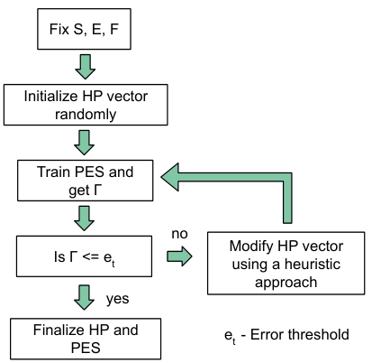
In inline optimization, a HP vector is chosen randomly and a preliminary ML-PES is trained and the response parameter (, RMSE) is computed. We either set a threshold value for the response parameter, or a maximum number of steps can be set alternatively. If is less than , then the optimal HP vector and corresponding ML-PES are obtained. If not, the HP vector is modified based on a heuristic algorithm and another ML-PES is trained with this modified HP set. This process is repeated until is below the threshold or the maximum number of steps are reached. This is the preferred approach if the PES training is not very expensive.
A popular HPO technique used in the ML community is Bayesian optimization (B-opt), Snoek et al. 2012 which is a hybrid of the inline and offline methodologies discussed above. B-opt requires a starting database of HP vectors and corresponding from which a surrogate function is built using GPR, similar to the offline optimization. A small number of samples compared to the offline optimization is enough to start B-opt. The surrogate function, which is also the objective function here, is defined exactly at the prior data points in the HP space while the estimated error in at other regions is given by a probability distribution function. An acquisition function is then generated based on the surrogate function and the associated error probabilities. This acquisition function shows us the most promising regions in the HP space to sample the next points. This aspect is similar to the inline optimization.
If the ML-PES training is costly and the HP space is huge, then all of the above techniques will be very time consuming. The classification schemes of the HPs discussed in the earlier section allow us to divide and conquer the HP space, but it will not help us reduce the cost of training ML-PESs. One solution to this problem is to train ML-PESs only using reference energies (i.e., leaving forces out) but evaluate them using both response parameters, and . It is to be noted that there will be regions in the HP space where one of the response parameters is minimal while the other is large, which are not optimal. By directing the search towards the regions in the HP space where both energy and force errors are minimal, we can obtain optimal HPs without explicitly training the models with forces.
Once optimal HPs are found, we can further improve the quality of ML-PES by refining the HP search, retraining the GAPs including forces. The rationale for leaving forces out of the fit in a first step is that there are a lot more reference forces than reference energies for a typical atomic structure data base. In particular, the number of reference energies equals the number of structures (i.e., “simulation boxes”) in the data base , whereas the number of forces equals times the average number of atoms in a structure. For a typical data base, the number of forces is therefore between one and two orders of magnitude larger than the number of energies. For the practical purposes of training a GAP, this means increasing CPU times and memory usage by the same relative amount.
Since GAPs can be trained cheaply by not including forces, we will use inline optimization to optimize our HPs. For this we will use a parallel particle swarm optimization (PPSO) algorithm, a heuristic based stochastic algorithm. An in house MPI Fortran implementation of the PPSO algorithm is used in this work. Our code is available free of charge at https://github.com/suresh0807/PPSO.git. There are 4 general steps in the PSO algorithm as follows:
1) Choose the number of particles in the swarm and initialize their positions in the user defined dimensional space and initialize their velocities to 0. Each HP coordinate () of a particle is chosen according to
| (14) |
Here, index runs from 1 through dimensions of the search space and is a random number between 0 and 1, which allows for an unbiased selection of the particle coordinates. and are the lower and upper bounds of the th HP, respectively.
2) For each particle (HP vector), train a GAP and compute the response variable(s). At , the initialized HP coordinates of each particle are labeled as the particle’s best location or simply local best (). From the swarm, the coordinates of the particle with the lowest response value are labeled as the global best (). At , the local best for each particle is the set of coordinates that particle visited since that had the lowest associated response value. Similarly, global best is the set of coordinates that resulted in the lowest response value for any particle in the swarm since .
3) Compute particle velocities for a time step using
| (15) |
Here,
and are the ‘self confidence’ and ‘swarm confidence’ factors, which usually take a value between 0 and 2. Setting allows the particles to search the space completely independently of each other (‘exploration’), whereas setting constrains the particles to move directly towards the global best particle in the swarm (‘exploitation’). In practice, setting both provides the best compromise between exploration and exploitation. The adjustable parameter provides a random perturbation in the velocity to assist in HP space exploration. can be adjusted to either speed up or slow down the particle.
4) Update the new position of the particles using
| (16) |
and go to step 2 for the next iteration. We have developed our own PSO implementation because of the need to include custom-built objective functions to target individual stages in ML-PES training. Moreover, our problem requires a unique parallelization strategy where both PSO algorithm and the objective function could run in parallel in a hybrid fashion, to get the high-throughput required in HPO.
In this work, we use the QUIP/GAP qui; Bartók and Csányi 2015 code built with the TurboGAP Caro 2019; tur libraries, to train GAP models based on the soap_turbo descriptor. We also use TurboGAP on its own to compute soap_turbo descriptors.
5 HPO Strategies
5.1 Optimization Cost
HP optimization will be performed in several PSO iterations. In each iteration, a set number of response variable evaluations will be made on the HP coordinates given by the PSO algorithm. There are two strategic ways to optimize these HPs: 1) optimize {HP} and {HP} together by minimizing the RMSE of the test set geometries; 2) optimize {HP} and {HP} separately in two subsequent stages. Option 1 is the most obvious and straightforward way to optimize the HPs, which by default takes into consideration the interaction between {HP} and {HP}. By contrast, option 2 is based on the assumption that the interaction between the two sets of HPs is negligible so that {HP} can be optimized first, followed by the optimization of {HP}GAP. Option 2 gives us a distinct advantage in terms of computational effort needed to optimize the HPs. The number of {HP} is usually larger than the number of {HP}, whereas the time required to train a GAP is much larger than the time needed to evaluate SOAP descriptors. If we could find a way to choose the best {HP} to describe the data set cheaply, i.e., without training GAPs, we would be able to search the relatively smaller GAP HP space faster and more thoroughly. Once the optimal SOAP basis set is chosen, techniques such as those mentioned in Ref. Imbalzano et al. 2018 can be applied to further reduce the number of descriptor functions within the basis set without sacrificing the quality of the descriptors.
For GAP, the RMSE as quality parameter is an obvious objective function to minimize. However, an appropriate objective function for finding the best SOAP is not obvious. This means that we need to devise a suitable objective function to optimize SOAP for a given database. Since the prospect of training-free HPO is very enticing, we will evaluate both options in this manuscript.
In strategy 1, the response variable is the RMSE (, ) of the test set and we will use the full HP search space (16 dimensional) to find the minima.
In strategy 2, optimization is done in two stages. In the first stage, SOAP HPs are optimized in the SOAP HP sub-space (12 dimensional, including ) by considering a SOAP kernel distribution property as the response variable (e.g., maximizing its standard deviation).
In the second stage of strategy 2, GAP HPs are optimized in the GAP HP sub-space (4 dimensional) with fixed SOAP HPs obtained from the first stage and using the RMSE of the test set as the response variable.
Strategy 2 requires relatively high computational effort per iteration (stage 1 and 2 combined) when compared to strategy 1. However, stage 1 of strategy 2 requires less computational effort per iteration than strategy 1 since SOAP evaluation is much cheaper than GAP training. Also, stage 2 of strategy 2 will require a lower number of iterations to converge than strategy 1 because the HP search space is much smaller for the former. This means that we will need to train less GAPs using strategy 2 than using strategy 1 in the entire PSO run. Therefore, there are advantages in using strategy 2 if GAP training is expensive. On the other hand, if the GAP training and RMSE computation are cheap, then strategy 1 should be optimal. Note that, in both strategies, need not be optimized if forces are not included in the training.
5.2 C Dimer System
To test our HPO strategies, as a first example, we choose a ‘toy’ data set of an isolated C dimer. Note that the scalar distance between the two C atoms is enough to completely describe the C dimer system. However, we use the SOAP descriptor in this analysis simply as a proof of principle and to compare the results with more complex data sets in the next section. There are 30 structures in our dimer data set, with C-C distances ranging from 0.8 Å to 3.7 Å, increasing in steps of 0.1 Å. Because of symmetry, both C atoms in a given dimer structure will have the same SOAP. The optimal SOAP will change systematically as we go from contracted dimer to stretched (dissociated) dimer, and this difference should be picked up by the SOAP kernel, i.e., the dot product between SOAP vectors of C atoms from any two structures raised to the power of . While is not formally a SOAP HP, we include it in {HP} since the kernel distribution is dependent on it.
5.2.1 Importance of {HP}
First of all, we want to showcase the impact of the shape affecting SOAP HPs on SOAP kernels and why it is important to optimize them for the data set at hand. Let us compare two sets of {HP}s with fixed values for , and rc Å, keeping constant at 147, and different values for the other HPs as listed in Table 2.
| {HP}SOAP | Set 1 | Set 2 |
|---|---|---|
| nmax | 6 | |
| lmax | 6 | |
| rch | 5.0 | |
| rcs | 4.21 | 3.40 |
| 0.69 | 0.13 | |
| 0.74 | 1.39 | |
| ar | 0.88 | 0.13 |
| at | 0.69 | 0.51 |
| a | 0.64 | 1.45 |
| cw | 0.53 | 1.26 |
| re | 0 | 2 |
| 1 | 1 | |
| Mean | 0.994 | 0.358 |
| Std | 0.008 | 0.379 |
| 10 | 10 | |
| Mean | 0.944 | 0.132 |
| Std | 0.075 | 0.280 |
The table also lists the resulting mean and standard deviation (std) of the corresponding kernel distribution at (linear kernel in the SOAP components) and at . Note that these two sets of HPs are somewhat arbitrary, having been chosen for the sole purpose of argumentation of how different, naively chosen, descriptor HP sets can lead to drastically different kernel distributions, and therefore drastically different ML model performance.
For the two SOAP HP sets, the similarity curves of 7 selected structures, as distinct from each other as possible in the data set, are compared in Figure 4 for and .
The corresponding kernel distributions are given in Figure 5. Please note that we use automatic range for x-axis based on the data as it also helps to see the range of similarity measures the kernel produces. As mentioned earlier, the kernel gives a similarity measure between 1 and 0, with 1 being exactly the same environment (up to symmetry operations) and 0 being nothing alike. Essentially, has the overall effect of scaling the kernel value. Larger values of emphasize the differences between atomic environments (make the kernel ‘sharper’). From Table 2, Figures 4a and 5a, we see that set 1 has a very narrow kernel distribution at (), and the mean close to 1 () means that the SOAP vectors from all the structures are very similar. A distribution that is symmetric about its mean value will have . Increasing the value of broadens the kernel distribution of set 1 (, ) by scaling down the kernel values, as seen in Table 2, Figures 4c and 5c. The numbers given above suggest that set 1 HPs do not result in a highly resolved SOAP since (i) all kernel values are for the linear kernel (Figure 5a) and for (Figure 5c); (ii) environments with C-C distance between 2.8 Å and 3.7 Å look very similar and the broadened kernel distribution at did not change the shape of the similarity curves either (Figures 4a and 4c).
In contrast with set 1, set 2 shows a reasonably broad kernel distribution () already at , with the kernel values spanning the full range between 0 and 1 (), as seen in Figures 4b and 5b. Here, set 2 linear kernel provides clearly distinguishable similarity curves for each environment.
Further increasing in set 2 leads to continued down scaling of the kernel values (; ) and results in the similarity measures falling steeply for almost all environments (Figures 4d and 5d). Set 2 HPs with large values will therefore result in under-fitting when used to train a GAP. For quantitative understanding, we trained C dimer GAPs on DFT energies and forces using the above four SOAP HP sets (with eV, = 2 meV/atom and =20 meV/Å). The corresponding energy and force RMSEs are shown in the respective panels in Figures 4 and 5. We see a direct correlation between the changes in the std of the kernel distribution and the training errors: large std leads to low errors and vice-versa.
Based on the above observations, std of SOAP kernel distribution is chosen as a response variable in optimizing the shape-affecting SOAP HPs. The distribution in Figure 5b, although spanning the entire kernel range, is skewed towards low similarity values. We will find out in the next section whether std is a good universal response variable for SOAP optimization or not. More importantly, this tells us that choosing a large basis set and cutoff ({HP}) does not automatically guarantee a reasonable SOAP description of the system without the careful selection of {HP}. Choosing the best {HP} is non-trivial even for the simple C dimer data set, as we have discussed above, and is best done by efficient optimization algorithms such as the parallel PSO described in the previous section. We will look at more complex data sets in later sections.
5.2.2 Strategy 1
We begin our HP optimization studies of C dimer data set with strategy 1, in which both SOAP and GAP HPs are optimized at the same time by minimizing a linear combination of the energy and force errors, here chosen as +(/30). This way the code optimizes HPs by minimizing both energy and force errors at the same time. Since the magnitude of the energy error is usually smaller than the magnitude of the force error (when expressed in eV and eV/Å, respectively), we downscale the force error contribution by a factor of 30, to give roughly equal importance to both errors in the response variable. We initialized 16 particles in the swarm and selected a self-confidence to swarm-confidence ratio of 1:2 to put more emphasis on exploitation of the global best HP coordinates in each swarm step. We would also like to see if a smaller SOAP basis set could offer similar quality of GAPs as the larger ones.
Therefore, we started two PSO runs, one with fixed values of (S6-1) and the other with (S4-1), to keep the total number of SOAP components constant at 147 and 50, respectively. We also fixed the hard cutoff at 5 Å and randomly initialized the values of the other HPs within the bounds given in Table 3.
| HPSOAP | LB | UB | S6-1 | S4-1 | S6-2 | S4-2 |
|---|---|---|---|---|---|---|
| nmax | 6/4 | 6 | 4 | 6 | 4 | |
| lmax | 6/4 | 6 | 4 | 6 | 4 | |
| rch | 5.0 | |||||
| rcs | 4.0 | 5.0 | 4.60 | 4.61 | 4.49 | 4.87 |
| 0.1 | 2.0 | 0.38 | 0.24 | 0.23 | 0.15 | |
| 0.1 | 2.0 | 1.28 | 1.43 | 1.22 | 1.08 | |
| ar | 0.0 | 2.0 | 1.06 | 0.59 | 1.20 | 0.56 |
| at | 0.0 | 2.0 | 0.05 | 1.20 | 0.32 | 0.18 |
| a | 0.0 | 2.0 | 1.41 | 0.98 | 1.52 | 0.34 |
| cw | 0.0 | 2.0 | 0.81 | 0.92 | 1.26 | 0.73 |
| re | 0 | 2 | 1 | 1 | 1 | 2 |
| 2 | 10 | 5.52 | 4.60 | 7.21 | 3.79 | |
| 0.1 | 5.0 | 3.50 | 2.49 | 4.24 | 4.31 | |
| 0.001 | 0.100 | 0.056 | 0.061 | 0.001 | 0.001 | |
| 0.001 | 0.100 | 0.001 | 0.001 | 0.014 | 0.024 | |
| K mean | 0.51 | 0.58 | 0.51 | 0.49 | ||
| K std | 0.35 | 0.32 | 0.37 | 0.39 | ||
| [meV/atom] | 0.6 | 0.6 | 0.6 | 0.5 | ||
| [meV/Å] | 14.8 | 14.6 | 15.3 | 15.1 | ||
The table also includes the optimized HPs for the two sets along with the minimum response variable (RMSEs) and mean and std of corresponding SOAP kernels.
We find that, for this extremely simple system, the two differently sized SOAP can be optimized to provide GAPs with almost the same accuracy, energy RMSE of 0.6 meV/atom and force RMSE of meV/Å. The SOAP kernel distribution and similarity curves of the 7 distinct C environments are shown in Figure 6 for the optimized SOAP HPs.
From Figures 6a and 6b, we find that both HP sets differentiate the C environments very well. From the kernel distributions in Figures 6c and 6d, we find that the similarity measures span the entire kernel range and the distribution is also broad (std of 0.32 for S4-1 and 0.35 for S6-1) and more symmetric than those in Figure 5.
5.2.3 Strategy 2
We proceed with the first stage of strategy 2 in which we employed a PSO run with 16 particles to obtain optimal {HP} values for this simple C dimer data set by maximizing the standard deviation of the SOAP kernel distribution. Again, we test the two differently sized SOAP bases with (S4-2 and S6-2, respectively) at fixed hard cutoff of 5 Å and random initialization of the values of the other HPs within the bounds given in Table 3.
Maximizing the std of the kernel distribution ultimately led to increased tail weights, i.e., the contributions close to 0 and 1 increased while the contributions in between diminished, as shown in Figure 7. Using such kernels in GAP training will result in under fitting. This implies that while a broad kernel distribution is important to better distinguish between chemical environments, it is not necessarily true that the broadest kernel distribution will give the best possible GAP. Therefore, instead of maximizing only the std of the kernel distribution, we chose to optimize the HPs by simultaneously maximizing std and minimizing the skew of the distribution.
The similarity curves of the 7 C-dimer environments and the kernel distributions (similar to Figure 6), obtained from the SOAP HPs that are optimized using the revised response variable, are shown in Figure 8; the corresponding HP coordinates are given in Table 3. From the table, we find that the kernel distributions of both sets look very similar in terms of the mean and std values, despite the fact that S4-2 has roughly 100 less SOAP components than S6-2. This suggests that HPO can be used to find the optimal size and shape of SOAP basis set for a given data set. In the next section we will find out whether this strategy also works for complex data sets.
To put our predictions to the test, we applied the PSO code to optimise GAP HPs (stage 2) within the ranges given in Table 3, while keeping the SOAP HPs fixed for the two cases. We used 20 particles per swarm, the same confidence ratio of 1:2 as before, and set the target response variable to +(/30). We used both energies and forces to train the GAPs. From Table 3, we see that both HP sets, S4-2 and S6-2, result in energy errors below 1 meV/atom and force errors below 20 meV/Å. The quality of the fits obtained from strategy 2 is comparable to those obtained from strategy 1. This indicates that our divide-and-conquer approach (strategy 2), to optimize SOAP and GAP HPs separately, works for this toy C dimer system.
5.3 Complex Data Sets
So far, we have tested our two proposed HPO strategies on a toy dimer system. We have identified that kernel distribution properties such as skewness and std can be used as response variables in obtaining optimal SOAP for a given data set. Now, we apply the two strategies to optimize SOAP and GAP HPs for already published amorphous carbon Deringer and Csányi 2017 and -iron Dragoni et al. 2017 data sets. It is to be noted that the optimal kernel distribution for condensed-phase systems may not look symmetric as in the case of the C dimer data set, as there will be a lot more environments that look similar (kernel value close to 1) than the ones that are completely dissimilar (kernel value close to 0). It will be interesting to see what kind of kernel distributions we arrive at by maximizing its std and minimizing its skewness.
The amorphous carbon (a-C) database consists of 4080 structures out of which there are 3070 bulk amorphous carbon structures, 356 crystalline structures, 624 amorphous surface geometries and 30 C dimer geometries (those studied in the previous section). There are a total of 256,628 C atomic environments in this database, and it includes several high energy structures with very high forces (ca. 100 eV/Å). Therefore, we should expect relatively larger energy and force errors for this system as compared to the simple dimer data set. The -Fe database consists of 12,171 structures in total, with 152,293 Fe atomic environments. The largest force value in this database is ca. 30 eV/Å.
If we denote the total number of atomic environments in a database be , then the total number of unique kernels that can be constructed is (where we have removed the trivial self-similarities). In our databases, this leads to a total of similarity checks in the order of . Handling this number of data points is intractable computationally (both in terms of CPU time and memory). Therefore, we have used 3000 randomly selected environments to construct the SOAP kernels, for a total of similarity checks, which is much more manageable. For the GAP fits, 4030 (a-C) and 4500 (-Fe) sparse environments () are chosen by decomposition, Mahoney and Drineas 2009 a low-rank matrix decomposition method, with 20% (a-C) and 30% (-Fe) of the structures in the data set randomly chosen per configuration type to make up the test set (TE), the rest making up the training set (TR). We have simply used a subset of the full data set as the test set, but a comprehensive test suite tailor-made for the specific system can also be employed here. Moreover, we reiterate that the GAP fits are trained only on reference energies, for computational efficiency, but the response is taken from both energy and force errors.
We tested the four optimal HP sets obtained in the previous section to find out whether they would perform well also for the condensed-phase system. We found that all of the four sets led to large errors for the a-C data set. Thus, there is no guarantee that the SOAP HPs that work well for one data set will be optimal for a different data set. Therefore, we must, in principle, optimize SOAP and GAP HPs for every new data set.
5.4 Amorphous Carbon Database
5.4.1 Strategy 1
For the complex a-C database, we test strategy 1 in which we optimized both SOAP and GAP HPs together within the bounds given in Table 4. Note that the GAPs are trained only on reference energies and not forces. Since we do not train with force information, HP need not be optimized.
| HPSOAP | LB | UB | aC6-1 | aC4-1 | Fe6-1 | Fe4-1 |
|---|---|---|---|---|---|---|
| nmax | 6/4 | 6 | 4 | 6 | 4 | |
| lmax | 6/4 | 6 | 4 | 6 | 4 | |
| rch | 5.0 | |||||
| rcs | 4.0 | 5.0 | 4.77 | 4.42 | 4.26 | 4.27 |
| 0.1 | 2.0 | 0.63 | 0.48 | 0.38 | 0.35 | |
| 0.1 | 2.0 | 0.50 | 0.17 | 0.68 | 0.22 | |
| ar | 0.0 | 2.0 | 0.003 | 0.03 | 0.05 | 0.81 |
| at | 0.0 | 2.0 | 0.02 | 0.12 | 0.20 | 0.12 |
| a | 0.0 | 2.0 | 1.30 | 1.98 | 1.20 | 1.36 |
| cw | 0.0 | 2.0 | 0.46 | 0.90 | 1.23 | 0.51 |
| re | 0 | 2 | 0 | 2 | 1 | 2 |
| 2 | 10 | 7.30 | 5.39 | 6.18 | 8.20 | |
| K mean | 0.87 | 0.86 | 0.99 | 0.99 | ||
| K std | 0.12 | 0.12 | 0.04 | 0.04 | ||
| K skew | 1.63 | 1.56 | 8.31 | 11.2 | ||
| nsparse | 4030 | 4500 | ||||
| 0.1 | 5.0 | 2.72 | 2.54 | 4.95 | 3.84 | |
| 0.001 | 0.100 | 0.010 | 0.015 | 0.001 | 0.001 | |
| [eV/atom] | 0.032 | 0.037 | 0.003 | 0.005 | ||
| [eV/Å] | 1.211 | 1.172 | 0.093 | 0.124 | ||
Table 4 also contains the optimized HPs for the two SOAP basis sizes, aC4-1 and aC6-1 with fixed at 5 Å. We were able to find optimal HPs for each of the sets providing similar test set errors. This suggests that by optimizing the HPs, a small SOAP basis can perform similarly to a larger basis, even for a complex data set. This amorphous carbon database consists of liquid carbon geometries with some large forces, thus the large errors and it is consistent with the values reported in the original paper. Deringer and Csányi 2017 In the original paper, the final potential is a combination of SOAP, 2-body and 3-body contributions, and was set to 3.7 Å. In our PSO test, we have only used SOAP contributions. However, it is straightforward to include the 2-body and 3-body HPs here, which will lead to a nominal increase in the computational cost per iteration.
As the next step, we look at the SOAP kernel distribution given by the two sets of optimal HPs in Figures 9a and 9b. As we anticipated, the kernel distribution is weighted heavily towards 1 with a mean value ca. 0.87 for both sets. We also notice that the range of similarity measure extends all the way down to 0 in both cases. Note that we use automatic range for x-axis based on the data. This is due to the fact that the frequency for large similarity measures are very high compared to that of small similarity measures. If 0.0 is visible in the x-axis then there is at least one kernel with 0 similarity.
To validate the use of std and skew of the kernel distribution as the response variable in stage 1 of strategy 2, we compare the kernel distributions of the HP configurations that gave large errors in Figures 9c and 9d. We find the non-optimal HPs (aC4-1b and aC6-1b) gave narrow kernel distributions, similar to the C dimer case, along with large skew, and they did not span the entire kernel space either. It appears that our SOAP optimization objectives, maximizing std and minimizing skewness of the kernel distribution, might work for the condensed phase systems as well.
5.4.2 Strategy 2
We execute stage 1 of strategy 2 using the smaller SOAP basis, aC4-2, as the test case to optimize SOAP HPs for the a-C data set within the bounds given in Table 4. By maximizing the std of the kernel distribution to 0.26 and minimizing its skewness to 0.30 using PSO, we obtained a set of optimal SOAP HPs, aC4-2, given in Figure 10a (HP values in figure caption).
The value of is pushed towards the upper bound of its chosen range by the optimization procedure, which is not surprising as increasing down scales the kernel values and widens their distribution. For comparison, we recomputed the kernel distribution by setting the value to 2 while keeping the other HPs constant (in Figure 10b). This distribution has a mean of 0.85, std of 0.13 and skew of 1.68, which is similar to the optimal distribution found in strategy 2 (Figure 9a).
Fixing the SOAP HPs, aC4-2 obtained in stage 1, we proceeded with stage 2 and obtained a GAP fit providing test set errors of eV/atom and eV/Å by optimizing GAP HPs ( eV, eV). aC4-2 with provided a fit with similar errors ( eV/atom and eV/Å using eV and eV) suggesting that, while large values allow for better differentiation of similar environments, they do not have a large effect on the quality of the GAP fits. The above observations prove that our strategy 2 can be employed to obtain reasonable GAPs from a pre-optimized SOAP for this complex a-C data set. The force errors are very large when compared to the energy errors. It should be possible to reduce the force errors by including force information to retrain the GAPs with the above optimized HPs, which we will investigate further below.
5.5 -Fe
The optimal set of SOAP and GAP HPs for the alpha-Fe database obtained by strategy 1 is given in Table 4.
For the two optimal HP sets Fe4-1 and Fe6-1, with differently sized SOAP, the energy and force errors obtained for the test set are much smaller than for the a-C database. One reason for this is that a-C database consists of many repulsive geometries with large forces, compared to the -Fe database. The other reason is that bonding is very complex in a-C, when compared to that in pure transition metals, and the amount of cohesive energy per bond (related to the ‘spring constants’ in traditional force fields) is much higher. For instance, compare the bulk modulus and coordination numbers of diamond ( GPa and 4) and -Fe ( GPa and 8), which means that in C materials each bond stores about 7.5 times more energy than in Fe. Therefore, the relative GAP errors are virtually the same for a-C and -Fe databases. By contrast, the optimized SOAP kernel distributions are much narrower for this database () than for the a-C database and do not span the entire kernel space, as shown in Figure 11.
Now we switch to stage 1 of strategy 2 to find a broad kernel distribution for the small SOAP basis. We found a SOAP HP set, Fe4-2 ( Å, Å, , , , , , and ), that gave a kernel distribution that spanned the entire kernel space with a relatively larger std of 0.07 and a skew of 8.5. Keeping this set of SOAP HPs fixed, we optimized the GAP HPs in stage 2 ( eV, eV) to get the test set errors, meV/atom and meV/Å. Again, strategy 2 provided similar test set errors as that of strategy 1 for the -Fe database.
5.6 Training with Forces
Using the optimal HP sets obtained in the last sections for the two complex data sets, we retrained the GAPs on both energies and all force components (with eV/Å; we did not employ PSO to optimize this HP due to the high computational cost and memory bottleneck) and the results are listed in Table 5.
| HP set | [eV/atom] | [eV/Å] | ||
|---|---|---|---|---|
| GAP trained on | GAP trained on | |||
| E only | E and F | E only | E and F | |
| aC4-1 | 0.037 | 0.075 | 1.172 | 0.682 |
| aC4-2 | 0.041 | 0.098 | 1.330 | 0.755 |
| aC6-1 | 0.032 | 0.057 | 1.211 | 0.650 |
| Fe4-1 | 0.005 | 0.006 | 0.124 | 0.098 |
| Fe4-2 | 0.005 | 0.007 | 0.170 | 0.083 |
| Fe6-1 | 0.003 | 0.004 | 0.093 | 0.105 |
On the one hand, we observe a significant reduction (roughly 50%) in the force RMSE for the a-C GAPs when compared to those trained on reference energies only. At the same time, the energy RMSE for these GAPs has roughly doubled. Possible reasons for this observation are that there are far more force data points than there are energies and we did not optimize with the other HPs. It is also possible to include only a fraction of the force data for training, which would also reduce the training cost. On the other hand, the force RMSEs for -Fe GAPs have improved only marginally. However, the energy RMSEs have not increased much. One outlier is observed for the -Fe HP set, Fe6-1, for which the retrained GAP gave a surprisingly larger force error as compared to the energy only fit, but the difference is very small (12 meV/Å).
5.7 QM9 Dataset
As a final test, we employed Strategy 1 to learn the potential energies of the open source QM9 dataset. Ramakrishnan et al. 2014 The QM9 dataset consists of 130831 molecules made up of up to 5 elements (C, H, O, N, F) as listed in Table 6.
| Elements | Mol. | Env. | Mol. 100 | Mol. 1000 |
|---|---|---|---|---|
| CF | 2 | 13 | ||
| CFH | 96 | 1491 | 2 | 1 |
| CFHN | 610 | 8536 | 4 | |
| CFHNO | 951 | 12170 | 4 | |
| CFHO | 250 | 3540 | ||
| CFN | 3 | 23 | ||
| CFNO | 11 | 96 | ||
| CH | 4890 | 106235 | 4 | 31 |
| CHN | 13903 | 247483 | 15 | 114 |
| CHNO | 64374 | 1099065 | 47 | 516 |
| CHO | 45713 | 880348 | 32 | 330 |
| CN | 4 | 27 | ||
| CNO | 21 | 171 | ||
| HN | 1 | 4 | ||
| HO | 1 | 3 | ||
| NO | 1 | 5 | ||
| Total | 130831 | 2359210 | 100 | 1000 |
In a recent benchmark study, Christensen et al. 2020 the atomic descriptor based spectrum of London and Axilrod–Teller–Muto (aSLATM) model was found to provide the lowest MAE (between 210 meV/molecule and 230 meV/molecule) for the entire dataset when only 100 molecules are used for training. We used PSO to optimize a set of SOAP and GAP HPs so as to obtain an even lower MAE for the entire dataset using specially chosen 100 molecules for training. The composition of the training dataset is given in Table 6. The selection of these 100 molecules was done by prescreening through many random combinations of 100 molecules, training a GAP on those (without HPO) and then testing on a small subset of the QM9 database (circa 10 % of the entire database). The combination of 100 molecules obtained this way was the one chosen for HPO and then tested on the entire QM9 dataset. We also performed a similar test using 1000 molecules (distributed as shown in Table 6) in the dataset, although these 1000 molecules were randomly chosen among those molecules that showed good learning power in the 100-molecule prescreening. Optimal selection of molecular samples to construct such small datasets is far from trivial, and there is current work in progress in our group in this regard. We will not explore this issue further in this paper.
The optimized SOAP and GAP HPs for the two training datasets are listed in Table 7. For the optimization we fixed a small SOAP basis of which results in 1050 SOAP components per atomic environment. If we had used a larger basis, say , then we would have had to compute 4100 SOAP components per environment. We also used a simple method to ‘compress’ the SOAP descriptors, consisting on retaining only some of the SOAP components (450 components in this case) followed by renormalization of the SOAP vectors, to speed up the calculation. The retained components are simply those that incorporate expansion coefficients corresponding to the first radial basis function (the one with the lowest associated singular value) in each species channel. For example, for a single-species soap_turbo descriptor, only components of the form are retained, and all others are dropped. From our experience, this trivial compression does not affect the quality of the GAPs too much. More information on compression schemes will be provided in a future article.
| HPSOAP | HP100 | HP1000 |
|---|---|---|
| nmax | 4 | 4 |
| lmax | 4 | 4 |
| rch [Å] | 4.0 | 4.0 |
| rcs [Å] | 3.65 | 3.41 |
| 0.48 | 0.33 | |
| 0.14 | 0.19 | |
| ar | 0.44 | 0.001 |
| at | 0.14 | 0.013 |
| a | 1.97 | 1.98 |
| cw | 0.67 | 0.40 |
| re | 1 | 1 |
| 2.23 | 4.43 | |
| nsparse | 2000 | 2000 |
| 4.17 | 4.67 | |
| [meV/molecule] | 0.001 | 0.02 |
| MAEE [meV] | 198 | 64.5 |
We also fixed the SOAP hard cutoff to 4 Å and the soft cutoff was allowed to be randomly chosen between 3 and 4 Å. 2000 sparse environments are chosen by decomposition for the interpolation. All other initial parameters are chosen randomly within the range of values presented for earlier studies.
At the end of the optimization, we obtained a MAE of 198 meV/molecule for the entire QM9 dataset using the 100 molecule training set and a MAE of 64.5 meV/molecule for the 1000 molecule training set. Our results are either similar to or better than the current best values in the literature. Christensen et al. 2020 As a next step, We checked whether the HP set trained on a smaller training data provides lower errors when used with larger training data. When the HP100 set is used to train on the 1000 molecule data set, the MAE went up to 84.3 meV/molecule. Similarly, when HP1000 set is used to train on the 100 molecule data set, the MAE came to 313 meV/molecule. This suggests that HPs must be optimized for a given training data set.
6 Conclusion
We have presented two strategies to automatically optimize the hyper-parameters (HPs) for ML-PES generation from a given data set, using SOAP descriptors and GAPs (although the methodology is general and can be readily extended to other descriptor types and ML architectures). A custom coded parallel particle swarm optimizer was employed to stochastically find the optimal set of HPs in both strategies. This code is freely available online for the community to make use of it. In strategy 1, both SOAP and GAP HPs were optimized at the same time by minimizing the test set RMSE. In strategy 2, the SOAP HPs are optimized first by maximizing the standard deviation and minimizing the skewness of SOAP kernel distribution, followed by the optimization of GAP HPs by minimizing the RMSE of the test set. Strategy 2 was ultimately more efficient than strategy 1 since it did not require many GAPs to be trained. Both strategies are validated using three data sets: a simple toy C-dimer data set, together with more complex amorphous carbon and -Fe data sets. Both strategies provided similar quality SOAPs and GAPs for all of the tested data sets. More importantly, smaller SOAP basis was optimized to provide similar quality of GAPs as that of larger SOAP basis for all data sets, with the associated reduction in computational costs. Strategy 1 was then used exclusively to train GAPs for predicting molecular energies of the QM9 dataset. We demonstrated the ability of PSO to find optimal HPs for QM9 dataset using a smaller SOAP basis and using as few as 100 molecules in the training set. Strategy 2 introduced in this paper can be employed to efficiently optimize HPs of new and complex data sets without much knowledge of the specific environments they contain. Techniques such as these are needed to realise fully automated ML-PES generation.
References
- Allen and Tildesley (2017) Allen, M. P.; Tildesley, D. J. Computer simulation of liquids; Oxford university press, 2017.
- Hollingsworth and Dror (2018) Hollingsworth, S. A.; Dror, R. O. Molecular dynamics simulation for all. Neuron 2018, 99, 1129–1143.
- MacKerell Jr (2004) MacKerell Jr, A. D. Empirical force fields for biological macromolecules: overview and issues. J. Comp. Chem. 2004, 25, 1584–1604.
- Marx and Hutter (2009) Marx, D.; Hutter, J. Ab initio molecular dynamics: basic theory and advanced methods; Cambridge University Press, 2009.
- Handley and Popelier (2010) Handley, C. M.; Popelier, P. L. Potential energy surfaces fitted by artificial neural networks. J. Phys. Chem. A 2010, 114, 3371–3383.
- Behler (2016) Behler, J. Perspective: Machine learning potentials for atomistic simulations. J. Chem. Phys. 2016, 145, 170901.
- Schmitz et al. (2019) Schmitz, G.; Godtliebsen, I. H.; Christiansen, O. Machine learning for potential energy surfaces: An extensive database and assessment of methods. J. Chem. Phys. 2019, 150, 244113.
- Mueller et al. (2020) Mueller, T.; Hernandez, A.; Wang, C. Machine learning for interatomic potential models. J. Chem. Phys. 2020, 152, 050902.
- Dral et al. (2020) Dral, P. O.; Owens, A.; Dral, A.; Csányi, G. Hierarchical machine learning of potential energy surfaces. J. Chem. Phys. 2020, 152, 204110.
- Deringer et al. (2019) Deringer, V. L.; Caro, M. A.; Csányi, G. Machine Learning Interatomic Potentials as Emerging Tools for Materials Science. Adv. Mater. 2019, 1902765.
- Liu et al. (2010) Liu, C.; Li, F.; Ma, L.-P.; Cheng, H.-M. Advanced materials for energy storage. Adv. Mater. 2010, 22, E28–E62.
- Butler et al. (2013) Butler, S. Z.; Hollen, S. M.; Cao, L.; Cui, Y.; Gupta, J. A.; Gutiérrez, H. R.; Heinz, T. F.; Hong, S. S.; Huang, J.; Ismach, A. F. et al. Progress, challenges, and opportunities in two-dimensional materials beyond graphene. ACS nano 2013, 7, 2898–2926.
- Fenton et al. (2018) Fenton, O. S.; Olafson, K. N.; Pillai, P. S.; Mitchell, M. J.; Langer, R. Advances in biomaterials for drug delivery. Adv. Mater. 2018, 30, 1705328.
- de Pablo et al. (2019) de Pablo, J. J.; Jackson, N. E.; Webb, M. A.; Chen, L.-Q.; Moore, J. E.; Morgan, D.; Jacobs, R.; Pollock, T.; Schlom, D. G.; Toberer, E. S. et al. New frontiers for the materials genome initiative. Npj Comput. Mater 2019, 5, 41.
- Schmidt et al. (2019) Schmidt, J.; Marques, M. R.; Botti, S.; Marques, M. A. Recent advances and applications of machine learning in solid-state materials science. Npj Comput. Mater 2019, 5, 1–36.
- Meredig (2019) Meredig, B. Five High-Impact Research Areas in Machine Learning for Materials Science. Chem. Mater. 2019, 31, 9579–9581.
- Morgan and Jacobs (2020) Morgan, D.; Jacobs, R. Opportunities and Challenges for Machine Learning in Materials Science. Annu. Rev. Mater. 2020, 50.
- Kohn and Sham (1965) Kohn, W.; Sham, L. J. Self-consistent equations including exchange and correlation effects. Phys. Rev. 1965, 140, A1133.
- Schran et al. (2018) Schran, C.; Uhl, F.; Behler, J.; Marx, D. High-dimensional neural network potentials for solvation: The case of protonated water clusters in helium. J. Chem. Phys. 2018, 148, 102310.
- Chmiela et al. (2018) Chmiela, S.; Sauceda, H. E.; Müller, K.-R.; Tkatchenko, A. Towards exact molecular dynamics simulations with machine-learned force fields. Nat. Commun. 2018, 9, 3887.
- Rupp et al. (2012) Rupp, M.; Tkatchenko, A.; Müller, K.-R.; Von Lilienfeld, O. A. Fast and accurate modeling of molecular atomization energies with machine learning. Phys. Rev. Lett. 2012, 108, 058301.
- Huo and Rupp (2017) Huo, H.; Rupp, M. Unified representation of molecules and crystals for machine learning. arXiv preprint arXiv:1704.06439 2017,
- Himanen et al. (2020) Himanen, L.; Jäger, M. O.; Morooka, E. V.; Canova, F. F.; Ranawat, Y. S.; Gao, D. Z.; Rinke, P.; Foster, A. S. DScribe: Library of descriptors for machine learning in materials science. Comput. Phys. Commun. 2020, 247, 106949.
- Christensen et al. (2020) Christensen, A. S.; Bratholm, L. A.; Faber, F. A.; Anatole von Lilienfeld, O. FCHL revisited: Faster and more accurate quantum machine learning. J. Chem. Phys. 2020, 152, 044107.
- Bartók et al. (2013) Bartók, A. P.; Kondor, R.; Csányi, G. On representing chemical environments. Phys. Rev. B 2013, 87, 184115.
- Caro (2019) Caro, M. A. Optimizing many-body atomic descriptors for enhanced computational performance of machine learning based interatomic potentials. Phys. Rev. B 2019, 100, 024112.
- Behler (2011) Behler, J. Atom-centered symmetry functions for constructing high-dimensional neural network potentials. J. Chem. Phys. 2011, 134, 074106.
- Willatt et al. (2019) Willatt, M. J.; Musil, F.; Ceriotti, M. Atom-density representations for machine learning. J. Chem. Phys. 2019, 150, 154110.
- Imbalzano et al. (2018) Imbalzano, G.; Anelli, A.; Giofré, D.; Klees, S.; Behler, J.; Ceriotti, M. Automatic selection of atomic fingerprints and reference configurations for machine-learning potentials. J. Chem. Phys. 2018, 148, 241730.
- Schütt et al. (2017) Schütt, K. T.; Arbabzadah, F.; Chmiela, S.; Müller, K. R.; Tkatchenko, A. Quantum-Chemical Insights From Deep Tensor Neural Networks. Nat. Commun. 2017, 8, 1–8.
- Behler and Parrinello (2007) Behler, J.; Parrinello, M. Generalized neural-network representation of high-dimensional potential-energy surfaces. Phys. Rev. Lett. 2007, 98, 146401.
- Bartók et al. (2010) Bartók, A. P.; Payne, M. C.; Kondor, R.; Csányi, G. Gaussian approximation potentials: The accuracy of quantum mechanics, without the electrons. Phys. Rev. Lett. 2010, 104, 136403.
- Bartók and Csányi (2015) Bartók, A. P.; Csányi, G. Gaussian approximation potentials: A brief tutorial introduction. Int. J. Quantum Chem. 2015, 115, 1051–1057.
- Bernstein et al. (2019) Bernstein, N.; Csányi, G.; Deringer, V. L. De novo exploration and self-guided learning of potential-energy surfaces. npj Comput. Mater. 2019, 5, 1.
- Bergstra et al. (2015) Bergstra, J.; Komer, B.; Eliasmith, C.; Yamins, D.; Cox, D. D. Hyperopt: a python library for model selection and hyperparameter optimization. Comput. Sci. Discov. 2015, 8, 014008.
- Abbott et al. (2019) Abbott, A. S.; Turney, J. M.; Zhang, B.; Smith, D. G. A.; Altarawy, D.; Schaefer, H. F. PES-Learn: An Open-Source Software Package for the Automated Generation of Machine Learning Models of Molecular Potential Energy Surfaces. J. Chem. Theory Comput. 2019, 15, 4386–4398, PMID: 31283237.
- Collet and Rennard (2008) Collet, P.; Rennard, J.-P. Intelligent information technologies: Concepts, methodologies, tools, and applications; IGI Global, 2008; pp 1121–1137.
- Feurer and Hutter (2019) Feurer, M.; Hutter, F. In Automated Machine Learning: Methods, Systems, Challenges; Hutter, F., Kotthoff, L., Vanschoren, J., Eds.; Springer International Publishing: Cham, 2019; pp 3–33.
- Cawley et al. (2005) Cawley, G. C.; Talbot, N. L. C.; Chapelle, O. Estimating predictive variances with kernel ridge regression. Machine Learning Challenges Workshop. 2005; p 56.
- Deringer and Csányi (2017) Deringer, V. L.; Csányi, G. Machine learning based interatomic potential for amorphous carbon. Phys. Rev. B 2017, 95, 094203.
- Anderson and Whitcomb (2000) Anderson, M. J.; Whitcomb, P. J. Design of experiments. Kirk-Othmer Encyclopedia of Chemical Technology 2000, 1–22.
- Hedayat et al. (2012) Hedayat, A. S.; Sloane, N. J. A.; Stufken, J. Orthogonal arrays: theory and applications; Springer Science & Business Media, 2012.
- Sobol’ (1967) Sobol’, I. On the distribution of points in a cube and the approximate evaluation of integrals. USSR Comput. Math. & Math. Phys. 1967, 7, 86 – 112.
- Kondati Natarajan (2020) Kondati Natarajan, S. DOE-offline-optimization. https://github.com/suresh0807/DOE-offline-optimization.git, 2020.
- Snoek et al. (2012) Snoek, J.; Larochelle, H.; Adams, R. P. Practical bayesian optimization of machine learning algorithms. Advances in neural information processing systems. 2012; pp 2951–2959.
- (46) QUIP. https://libatoms.github.io, Accessed: 2020-08-17.
- (47) TurboGAP. https://turbogap.fi/wiki/index.php/Main_Page, Accessed: 2020-08-17.
- Dragoni et al. (2017) Dragoni, D.; Daff, T. D.; Csányi, G.; Marzari, N. Gaussian Approximation Potentials for iron from extended first-principles database (Data Download), Materials Cloud Archive 2017.0006/v2 (2017). https://archive.materialscloud.org/record/2017.0006/v2, 2017.
- Mahoney and Drineas (2009) Mahoney, M. W.; Drineas, P. CUR matrix decompositions for improved data analysis. Proc. Natl. Acad. 2009, 106, 697–702.
- Ramakrishnan et al. (2014) Ramakrishnan, R.; Dral, P. O.; Rupp, M.; von Lilienfeld, O. A. Quantum chemistry structures and properties of 134 kilo molecules. Scientific Data 2014, 1.