Dynamical Phase Error in Interacting Topological Quantum MemoriesPreprint: DIAS-STP-21-07
![[Uncaptioned image]](2101.00022v2/ORCID.png) S. Dooley
I. Jubb
K. Kavanagh
G. Kells
S. Dooley
I. Jubb
K. Kavanagh
G. Kells
Abstract
A local Hamiltonian with Topological Quantum Order (TQO) has a robust ground state degeneracy that makes it an excellent quantum memory candidate. This memory can be corrupted however if part of the state leaves the protected ground state manifold and returns later with a dynamically accrued phase error. Here we analyse how TQO suppresses this process and use this to quantify the degree to which spectral densities in different topological sectors are correlated. We provide numerical verification of our results by modelling an interacting p-wave superconducting wire.
I Introduction
Topological schemes to protect and manipulate quantum information are based on fractional excitations called anyons. In these approaches information is stored in anyon pairs and, by moving them apart, one can encode this information in a non-local way Kitaev 2001; Dennis et al. 2002; Kitaev 2003; Kitaev 2006; Nayak et al. 2008; Stanescu and Tewari 2013. This is the key feature that allows topological memories to be robust against local noise and decoherence processes.
In these topological platforms the computational space is a degenerate ground state manifold that emerges when these quasi-particle excitations are far apart (see Fig. 1). The degeneracy of this subspace is fundamentally important because it protects against quantum memory corruption in the form of unwanted qubit rotations, which arise via the accumulation of relative dynamical phases. This feature of the ground state manifold arises from a more general property called Topological Quantum Order (TQO) Wen and Niu 1990; Wen 1990; Hastings and Wen 2005; Bravyi et al. 2010; Zeng et al. 2019. Among other things, TQO implies that, for states within this manifold, the expectation values of local observables are equal up to some exponentially small correction that depends on the spatial separation between anyons.
Another mechanism which can corrupt the quantum memory with undesirable qubit rotations is dynamical phase error. This can occur when the quantum state partially leaves the ground state manifold and returns later with a dynamically altered phase. This type of error could arise on a mean-field level if there are causally connected perturbations near different anyons Conlon et al. 2019. In this scenario the distance between anyons plays an important role in delaying/reducing the onset of this type of secondary error process. In interacting systems however, a different scenario for phase error still exists because the aforementioned ground state degeneracy does not necessarily extend to a degeneracy in bulk eigenstates. One could then reasonably worry about processes whereby a single localised perturbation creates, and then at a later time, returns an excitation that has accumulated some relative dynamical phase from its time spent in the energy mismatched bulk.

In this paper we show that, despite a mismatched bulk spectrum, TQO guarantees that such interaction driven phase errors are suppressed up to a time that scales with system size. A consequence of this suppression is that, although the bulk spectra from distinct topological sectors differ, there is necessarily a high degree of correlation between spectral densities. This correlation can be quantified by considering appropriate Green’s functions.
We demonstrate these general results, for any system with TQO, using a concrete example: a Majorana based topological memory based on interacting p-wave superconducting wires Fu and Kane 2008; Lutchyn et al. 2010; Oreg et al. 2010; Clarke et al. 2011; Alicea et al. 2011, as shown schematically in Fig. 1 (c). In this setting we back up our key claims using a TDVP-MPS approach Haegeman et al. 2011; Paeckel et al. 2019 which allows us to: (1) show that, even in regimes where interactions and time-dependent perturbations are relatively strong, there is no phase error other than what one would expect from mean-field like effects, and (2) directly calculate spectral densities in each topological sector and quantitatively demonstrate the degree of correlation that must exist between them.
II No phase error argument
Consider some gapped local Hamiltonian 11 1 By local Hamiltonian we mean a sum of Hermitian operators that are each only non-trivial on several neighbouring sites. with anyonic quasi-particles. For simplicity, we assume there are two ground states, and , corresponding to (e)ven and (o)dd parity respectively 22 2 This is the case for the Majorana example below. It is straightforward to generalise the argument to a higher dimensional ground state manifold.. Crucially, we assume that for large enough system diameter , there is a length that scales in some way with (this length must satisfy for some constant ), for which the ground states satisfy the TQO property:
For every local operator, , supported in a region of diameter at most , we have
| (1) |
for some constant . That is, local operators cannot be used to distinguish the two sectors, up to exponential corrections in .
From the TQO property one can see that the ground states are degenerate, up to exponential corrections in the system length Bravyi et al. 2010; Bravyi and Hastings 2011. That is, is approximately the same for 33 3 is a sum of a polynomial (in ) number of -local terms, . TQO implies that is sector independent up to , which dominates the polynomial in in the sum .. Although TQO makes no direct claims on the behaviour of states above the gap that separates the ground state manifold from the bulk excited states, it can be used however to derive certain properties see e.g. Bravyi et al. 2010. In what follows we show how TQO bounds the dynamically driven phase error, and how this results in a large number of constraints on the bulk spectrum.
We consider two instantaneous local perturbations of the system, separated by a time . The unitary evolution operator in this case is: where and are local Hermitian operators (possibly at different locations) that do not mix the even and odd sectors. By a phase error we mean that is different for the even and odd sectors. We can expand in the energy eigenstates, , to get
| (2) |
where is the energy of the eigenstate in the -sector. For special cases, where there is a degeneracy between the two sectors for all bulk energies, i.e. , and where the overlaps are sector independent, there is no phase error. Neither condition necessarily holds for an interacting system. Nevertheless, one can make the following argument for the suppression of phase error.
First, we write
| (3) |
where we have defined , and we have used where, by the approximate ground state degeneracy, is exponentially close between the sectors. From the Lieb-Robinson bounds Lieb and Robinson 1972 we note that we can approximate by an operator , supported in a region of size about , up to corrections of order 44 4 Our argument involves several exponential error terms; each with its own rate constant . To avoid ambiguity, we take to be the smallest such constant such that each error estimate is valid.. Here is the Lieb-Robinson speed of propagation for . We can then pick some , such that the maximum size of over the range of times is at most , and such that approximates to order . There are two cases to consider:
i) If is contained in an sized region about for sufficiently large , then, for all times , is contained in a region of size at most . TQO then implies that is sector independent to order . Putting everything together, for times we find that is approximately equal between the sectors, up to exponential corrections in . In this situation we say there is no phase error.
ii) If is not contained in an sized region about , then the separation between and must be growing with . The fact that the system is gapped means that , up to an exponential correction in the operator separation (Hastings 2004; Hastings and Koma 2006), and hence of order . For the TQO condition implies that is sector independent up to exponential corrections, and hence is too. That is, we again have exponentially vanishing phase error for times .
Note that the exact time, , for which no phase error arises, depends upon the specific system, the perturbations, and their separation. The preceding argument should be understood as heuristic justification that scales as , and hence as . In Sec. II.1 we address the general scenario of time-dependent perturbations, and we make similar arguments for phase error suppression.
The suppression of phase error implies a large number of constraints on the bulk spectra in the following way. From (2) we can write the amplitude of the phase error, denoted here by , as:
| (4) | ||||
where , and the sum runs from as the ground state contribution is contained in the exponential correction on the far RHS. Above we showed that is exponentially suppressed. This then implies that the magnitude of difference between the even and the odd sums (for ) on the RHS is also exponentially suppressed in . Crucially, this is also the case for many pairs of local operators, and , though the exact form of the suppression may differ in each case. One can then consider this constraint between the even and odd sums for all such pairs, resulting in a substantial number of constraints. The effect of this on the bulk splittings is illustrated in Sec. III for a specific model.
II.1 No Phase Error for Time-Dependent Perturbations
Here we generalize the no phase error argument to time-dependent perturbations. Consider a time-dependent local perturbation . The time-ordered unitary evolution operator is then
| (5) |
To show there is no phase error we need to show that is approximately sector independent. As is not a local operator we cannot immediately use the TQO condition. However, we can turn it into a local operator times a non-local operator that acts trivially on the system eigenstates:
| (6) |
where , which essentially follows from the interaction picture.
From the Lieb-Robinson bounds, we can approximate , and hence the time-ordered unitary involving , by an operator supported in a region of size , up to corrections of order . Thus, we have
| (7) |
where is the same in both sectors up to corrections of order . For , we make an error of order by approximating the time-ordered unitary in a region of size . In doing so we can then use TQO to argue that the expectation value on the last line is sector independent to order , and hence is too, i.e. no phase error.
If we now include a second time-dependent perturbation , separated from such that up to exponential corrections in the separation between and , then the unitary approximately factorises as
| (8) |
It is straightforward to apply the gap argument from above to show that this will also not incur a phase error for .
III A Majorana-based Example
To demonstrate these general results we model a simple topological memory consisting of two one-dimensional p-wave superconducting wires separated by a potential barrier, as shown in Fig. 1 (c). The -site ( sites each for the left and right wires) lattice Hamiltonian Kitaev 2001 for this is given by:
| (9) |
where is the superconducting gap, is the on-site chemical potential, is the potential profile, see App. A, is the hopping parameter and the represent fermion (creation) annihilation operators. Interactions are modelled using a nearest-neighbour density-density term:
| (10) |
where is the interaction strength. The fully interacting Hamiltonian of interest is . This model can be effectively realized in proximity coupled systems Fu and Kane 2008; Lutchyn et al. 2010; Oreg et al. 2010; Clarke et al. 2011; Alicea et al. 2011; Stanescu and Tewari 2013 which are backed up with extensive experimental evidence Mourik et al. 2012; Deng et al. 2012; Das et al. 2012; Finck et al. 2013; Churchill et al. 2013; Albrecht et al. 2016; He et al. 2017; Deng et al. 2016; Nadj-Perge et al. 2014; Ruby et al. 2015; Pawlak et al. 2016; Zhang et al. 2018; Fornieri et al. 2019; Ren et al. 2019. For discussions on different types of noise that can occur in these systems see Rainis and Loss 2012; Budich et al. 2012; Roy et al. 2012; Konschelle and Hassler 2013; Yang and Feldman 2014; Ng 2015; Pedrocchi and DiVincenzo 2015; Hu et al. 2015; Ippoliti et al. 2016; Brown et al. 2016; Aseev et al. 2018; Knapp et al. 2018; Zhang et al. 2019; Karzig et al. 2013; Scheurer and Shnirman 2013; Conlon et al. 2019; Coopmans et al. 2021.
The non-interacting Hamiltonian, , gives rise to four Majorana zero-energy modes Kitaev 2001, localised at the domain walls between topological () and non-topological regions encoded by , which can be paired into two Dirac fermionic zero-modes ), one for the left () and one for the right wire (). From the 4-fold degeneracy associated with these zero-modes we can, without loss of generality, define our topologically protected ground states from the even-parity sector (states with an even number of excitations) as:
| (11) |
in which corresponds to the ground state of the bulk modes and are the respective unoccupied and occupied Dirac zero-mode for the wire. In what follows we will effectively forget about the right wire. Its purpose is to keep us in the even-parity sector overall. Henceforth, any mention of even and odd sectors, and wires, will refer to the left wire only.
When local interactions are present () we can no longer label many-body eigenstates of in terms of their quasi-particle occupation numbers. However, it can be shown that the topological ground state degeneracy holds (up to exponential corrections in the length of the system) provided that the interactions do not close the gap Moon and Nachtergaele 2018, and that the system satisfies the TQO property. However, the same degeneracy between the excited states can be broken by interactions when the spectrum contains overlapping quasi-particle bands Kells 2015a; Moran et al. 2017; Kells et al. 2018; Pellegrino et al. 2020, leaving open the possibility for phase errors to be returned to the ground state without the need for quasi-particle propagation. The results presented here are focused solely upon such dynamically generated phase errors due to bulk energy mismatches. However, based on our argument in the previous section, this mechanism must be suppressed because has TQO as shown in App. B.
III.1 Numerical Verification
To support our analytical argument we now present numerical results for the more general case of a time-dependent perturbation. Specifically, we simulate an oscillating perturbation on the left boundary of the Majorana wire, see App. A. We quantify the phase error as
| (12) |
in what follows. Note that corresponds to no phase error.
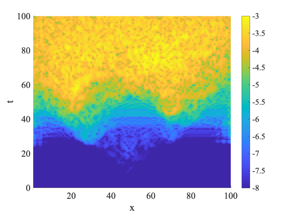
Our numerical results are obtained using time-dependent-variational-principle (TVDP) matrix product state (MPS) simulations Haegeman et al. 2011; Paeckel et al. 2019. In Fig. 2, we examine the time-averaged rate of phase error as a function of the the time-averaged energy difference, , between the approximately degenerate ground states for finite size systems 55 5 The ground state energy splitting is time-averaged because the spectrum to varying in time due to the time-dependent perturbation.. The results clearly show that the numerical methodology is capable of detecting phase error in the dynamics once the ground state splitting is of order . When the system is large enough, such that interactions do not make a detectable change to , no systematic increase in phase error occurs.
We also consider the case of a second oscillating perturbation at the right boundary of the wire. Fig. 3 shows that in this case, after a time there is a sudden increase in phase error. This is well understood on a mean field level: excitations originating at one wall return to the ground state space at the other wall, generating a error in the ground state space (see, e.g., Scheurer and Shnirman 2013; Conlon et al. 2019). Crucially, before we see no evidence of any other systematic phase error, other than that attributable to the splitting in the ground state manifold.
In addition to these phase error results we also provide some numerical TDVP-MPS simulation results for the qubit-loss error (infidelity) as defined by
| (13) |
In Fig. 4 we show the response of the system to a single oscillating boundary across a range of frequencies from the almost adiabatic regime, , up to frequencies far in excess of the topological gap. The results resemble the expected local density of states in the wire, in a given parity sector. We see that repulsive interactions lower the peak resonant frequency (in agreement with an expected reduction to the band edge). We also see that the topological memory degrades slightly across all frequencies. This is somewhat different from what is observed in non-interacting studies, where a lower bulk gap from, say from a reduced p-wave pairing or a lower wire electron density, can result in an improved robustness to high-frequency perturbations Conlon et al. 2019.
IV Spectral correlation
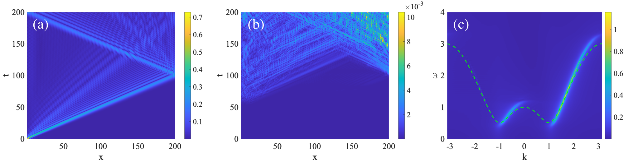
Notably, the deviations observed in phase error after are not driven by the phase error accumulated in the bulk states, but are associated with the fact that the dynamics eventually make local operators non-local. However, the fact that we cannot observe phase error before , for all initially local perturbations, implies that the even-odd excited energy spectra in the interacting model are related in some way that is unique to systems with TQO. This is most clearly demonstrated by Fourier transforming the system’s Green’s functions.
Consider for example taking and in and define the Green’s function for the -sector as
| (14) |
which depends on the operator positions, and , and the time . For convenience, we fix (the left boundary of the wire) or (the middle of the wire) and consider as a function of only.
No phase error implies that the difference, is exponentially suppressed for times , and hence so is the integral of over . One can then verify that this implies that the Fourier transform, , is exponentially suppressed when convolved with the Fourier transform, , of some cut-off or box function, e.g. for and otherwise. In other words, while the spectral functions, , differ between sectors, these differences are washed out by smearing, or convolving, with 66 6 For a box function, with cut-off , has the form of a sinc function of width , and hence a convolution with acts to smear by this width in the direction.. It is important to note that this is not a perturbative statement.
IV.1 Extension to fermionic operators
The analytical arguments above rest heavily on the Lieb-Robinson bounds, which are formulated as commutation relations between local operators. Fermionic operators such as are non-local, as they can be seen as strings of local operators through the Jordan-Wigner representation. Even powers of such fermionic operators, on the other hand, are local. Our analytical results, therefore, only pertain to the latter, and hence only address time-dependent changes within parity preserving Hamiltonians.
Despite this, in Fig. 5 we illustrate the Green’s functions and their FT’s for fermionic operators and . The resulting resolution in reciprocal space is of the order ]. One can estimate from Fig. 3 that the Lieb-Robinson speed , and hence, while increased interactions imply a coarser grained energy correlation between sectors, making the system larger allows us to systematically improve this bound. For details on how similar arguments can apply to multiparticle Green’s functions see App. C for further discussion. The numerical results, in particular the cancellations of even and odd Green’s functions up to a time (Fig. 5 (b)), indicate that it may be possible to extend the analytical argument to fermionic perturbations. The work in Nachtergaele et al. 2018; Hastings and Koma 2006 likely offers a good starting point for such generalisations.
V Conclusion
We have shown that in systems possessing TQO dynamical driven phase-errors are suppressed which implies that spectral densities in different topological sectors are always highly correlated. This result offers a useful baseline for research into strong zero-modes and high-temperature properties of topological memories. Although the bounds presented are weaker than the special cases of strong zero-modes Gangadharaiah et al. 2011; Jermyn et al. 2014; Kells 2015a; Kells 2015b; Fendley 2016; Kemp et al. 2017; Moran et al. 2017; McGinley et al. 2017; Mahyaeh and Ardonne 2018; Pellegrino et al. 2020; Mahyaeh and Ardonne 2020, they are both general and non-perturbative, applying to any material that satisfies the TQO condition. This is important, given the growing number of novel materials with topological features Bradlyn et al. 2017 of which some may satisfy the TQO condition.
More generally it might be possible to tighten rigorous bounds such as Bravyi et al. 2010 and make contact with works concerning disorder and constrained thermalisation e.g. Huse et al. 2013; Else et al. 2017; Kells et al. 2018; Nulty et al. 2020. Although it is well established that disorder prevents stray excitations propagating across a system (see e.g. Conlon et al. 2019), for free-fermion systems there is no evidence of a reduction in the propagation time itself. The situation could be very different in interacting environments and so a TDVP-MPS examination of this scenario would be an interesting avenue for further study.
Acknowledgements
We would like to acknowledge D. Pellegrino, A. Conlon, J. K. Slingerland, A. Romito, D. Meidan, F. Pientka and A. Werner for fruitful discussions, and A. Kells for her artistic renderings. L.C., K.K., S.D., and G.K. acknowledge Science Foundation Ireland for financial support through Career Development Award 15/CDA/3240. G.K. was also supported by a Schrödinger Fellowship. IJ is supported by a Schrödinger Scholarship.
Appendix A Potential profile
We simulate the two-wire setup of the Majorana based topological memory by utilising the potential profile:
| (15) |
where , for , encodes the lattice site positions of 4 domain walls, and is a Sigmoid function. We also choose the separating potential, and separation , to be large enough so as to render both wires fully disconnected. Note that any time-dependent noise protocols above only influence the left wire, and we assume that all low energy bulk excitations occur only in the left wire.
In Fig. 2 and 3 in the main text we oscillate the walls of the left wire. This is implemented by replacing with a time-dependent function , with a velocity and frequency that does not break
(super-)adiabaticity Karzig et al. 2013; Scheurer and Shnirman 2013; Conlon et al. 2019; Coopmans et al. 2021.
Appendix B TQO inheritance
Here we apply the arguments in Hastings and Wen 2005 to show how the interacting Majorana wire, , inherits approximate TQO (Eq. 1 in the main text) from some simpler system, denoted here by , with exact TQO. That is, the expectation values of any sufficiently local operator in the even and odd ground states of are exactly equal. For to inherit TQO from we require the two Hamiltonians to be quasi-adiabatically connected via a local process that does not close the gap.
There are several choices for that satisfy these requirements. For particular parameters, (the non-interacting wire Eq. 9 in the main text) has exact TQO for any operator of size at most Kitaev 2001, and one can tune from to by locally tuning the interaction strength and the other parameters in Eqs. 9 and 10 in the main text in a way that does not close the gap.


A more useful choice for , due to its proximity to in parameter space, is a partially interacting wire. Specifically, we tune the couplings on one side of the wire (say the right) to what we refer to as the special local Kitaev limit, denoted by , where , and (recall that the ’th site refers to the last site of the left wire). In this limit there are interactions throughout all of the wire except the last two sites, which allows a fully decoupled Majorana to sit on the right hand edge, and thus guarantees a precise even-odd degeneracy for all many-body states Kells 2015a. In the same way, is guaranteed to satisfy the exact TQO condition for operators of size at most , i.e. the entire length of the wire except a single site. The fact that our fully interacting system of interest, , differs from on a single site, means that it is relatively easy to quasi-adiabatically connect the two. This manifests in the approximate TQO condition of (Eq. 1 in the main text) as a smaller exponential error than would arise from a longer quasi-adiabatic path to .
Taking , we now follow Hastings and Wen 2005 to derive approximate TQO for . Denoting the ground states of as (for ), we have the exact TQO condition: for every local operator supported in a region of size at most . We consider a 1-parameter family of Hamiltonians , where and , where is the time we tune for. In Hastings and Wen 2005 they define a unitary operator, denoted here by , that quasi-adiabatically transitions between and . We only consider cases for which remains gapped throughout the tuning process Moon and Nachtergaele 2018. Since this is a local process, is always a sum of local terms.
Following Hastings and Wen 2005, we consider some local observable . We then form , which only acts on sites within a distance from the support of . Specifically, is the partial trace (up to some constant) of over all sites more than a distance from the support of . One can then show that,
| (16) |
where is some constant, and is a unitary operator acting only within the ground state manifold.
To use the exact TQO of the local limit in the RHS above, we require to be supported in a region of size at most . If the length of is , then the length of is , which is less than or equal to if . To connect up with Eq. 1 in the main text, we further assume that , where is some length satisfying , for some constant . At worst we then have , and hence the error above is order , for some (possibly different) constant .
Finally, given the exact TQO of the special local Kitaev limit, and the fact that only acts within the ground state manifold, we find that the expectation value, , is the same for both sectors. For the fully interacting Majorana system, , this implies that is the same for both sectors, up to for operators of size at most . This is the approximate TQO condition in Eq. 1 in the main text.
While the above argument concerned the special local Kitaev limit and a locally connected , it is clearly applicable to any pair of locally connected (gapped) systems where one is known to satisfy an exact TQO condition. This is of course also true more generally for higher dimensional ground state manifolds satisfying the same condition.
Appendix C Extension to multi-particle Green’s functions
Here we show some results for the 2-particle spectral densities. We set and in in Eq. 6 in the main text and define the Green’s function for the -sector as
| (17) |
which depends on the operator positions, and , and the time . We also fix (the middle of the wire) so as to not couple to the zero-modes (which tends to blur our spatial Fourier transform) and then plot and the difference , which is given in a log scale for clarity. Fig. 6(a) shows, up to numerical errors of that is exponentially suppressed for some initial time . Furthermore, this time scales with the system size .
Fig. 6(b) shows the shape of the 2-particle spectral density as a function of the total momentum, after cutting off the Green’s function for . Fig 6(b) can be compared against the exact density determined from the single particle solutions of a periodic system, given in Fig. 6(c).
The energetic resolution obtained in Fig. 6(b) is effectively governed by the Lieb-Robinson velocity and . However, as we stressed above in the constraints section, we are free to choose from a large number of local operators with which we can generate a much larger set of spectral constraints (Eq. 4 above). For example, we could generate the entire 3-parameter functions and perform a 2D Fourier transform on the first two spatial components, from which we could obtain a tighter -space resolution. In further Supplementary Material we provide two animated GIF files showing how this affects things for different momentum slices for the even and odd sectors. While the methodology still suffers from numerical artifacts, our key point is that movies are the same up to exponentially small corrections when the cut-off is enforced by an appropriate choice of .
References
- Kitaev (2001) A. Y. Kitaev, “Unpaired majorana fermions in quantum wires,” Physics-Uspekhi 44, 131 (2001).
- Dennis et al. (2002) E. Dennis, A. Y. Kitaev, A. Landahl, and J. Preskill, “Topological quantum memory,” Journal of Mathematical Physics 43, 4452–4505 (2002), https://doi.org/10.1063/1.1499754 .
- Kitaev (2003) A. Y. Kitaev, “Fault-tolerant quantum computation by anyons,” Annals of Physics 303, 2 – 30 (2003).
- Kitaev (2006) A. Y. Kitaev, “Anyons in an exactly solved model and beyond,” Annals of Physics 321, 2 – 111 (2006).
- Nayak et al. (2008) C. Nayak, S. H. Simon, A. Stern, M. Freedman, and S. Das Sarma, “Non-abelian anyons and topological quantum computation,” Rev. Mod. Phys. 80, 1083–1159 (2008).
- Stanescu and Tewari (2013) T. D. Stanescu and S. Tewari, “Majorana fermions in semiconductor nanowires: fundamentals, modeling, and experiment,” Journal of Physics: Condensed Matter 25, 233201 (2013).
- Wen and Niu (1990) X. G. Wen and Q. Niu, “Ground-state degeneracy of the fractional quantum hall states in the presence of a random potential and on high-genus riemann surfaces,” Phys. Rev. B 41, 9377–9396 (1990).
- Wen (1990) X.G. Wen, “Topological Order in Rigid States,” Int. J. Mod. Phys. B 4, 239 (1990).
- Hastings and Wen (2005) M. B. Hastings and X. G. Wen, “Quasiadiabatic continuation of quantum states: The stability of topological ground-state degeneracy and emergent gauge invariance,” Phys. Rev. B 72, 045141 (2005).
- Bravyi et al. (2010) S. Bravyi, M. B. Hastings, and S. Michalakis, “Topological quantum order: Stability under local perturbations,” Journal of Mathematical Physics 51, 093512 (2010), https://doi.org/10.1063/1.3490195 .
- Zeng et al. (2019) B. Zeng, X. Chen, D.L. Zhou, and X.G. Wen, Quantum Information Meets Quantum Matter: From Quantum Entanglement to Topological Phases of Many-Body Systems, Quantum Science and Technology (Springer New York, 2019).
- Conlon et al. (2019) A. Conlon, D. Pellegrino, J. K. Slingerland, S. Dooley, and G. Kells, “Error generation and propagation in majorana-based topological qubits,” Phys. Rev. B 100, 134307 (2019).
- Fu and Kane (2008) L. Fu and C. L. Kane, “Superconducting proximity effect and majorana fermions at the surface of a topological insulator,” Phys. Rev. Lett. 100, 096407 (2008).
- Lutchyn et al. (2010) R. M. Lutchyn, J. D. Sau, and S. Das Sarma, “Majorana fermions and a topological phase transition in semiconductor-superconductor heterostructures,” Phys. Rev. Lett. 105, 077001 (2010).
- Oreg et al. (2010) Y. Oreg, G. Refael, and F. von Oppen, “Helical liquids and majorana bound states in quantum wires,” Phys. Rev. Lett. 105, 177002 (2010).
- Clarke et al. (2011) D. J. Clarke, J. D. Sau, and S. Tewari, “Majorana fermion exchange in quasi-one-dimensional networks,” Phys. Rev. B 84, 035120 (2011).
- Alicea et al. (2011) J. Alicea, Y. Oreg, G. Refael, F. von Oppen, and M. P. A. Fisher, “Non-abelian statistics and topological quantum information processing in 1d wire networks,” Nature Physics 7, 412 EP – (2011).
- Haegeman et al. (2011) J. Haegeman, J. I. Cirac, T. J. Osborne, I. Pižorn, H. Verschelde, and F. Verstraete, “Time-dependent variational principle for quantum lattices,” Phys. Rev. Lett. 107, 070601 (2011).
- Paeckel et al. (2019) S. Paeckel, T. Köhler, A. Swoboda, S.R. Manmana, U. Schollwöck, and C. Hubig, “Time-evolution methods for matrix-product states,” Annals of Physics 411, 167998 (2019).
- (20) By local Hamiltonian we mean a sum of Hermitian operators that are each only non-trivial on several neighbouring sites.
- (21) This is the case for the Majorana example below. It is straightforward to generalise the argument to a higher dimensional ground state manifold.
- Bravyi and Hastings (2011) S. Bravyi and M. B. Hastings, “A short proof of stability of topological order under local perturbations,” Communications in Mathematical Physics 307, 609 (2011).
- (23) is a sum of a polynomial (in ) number of -local terms, . TQO implies that is sector independent up to , which dominates the polynomial in in the sum .
- Lieb and Robinson (1972) E.H. Lieb and D.W. Robinson, “The finite group velocity of quantum spin systems,” Commun. Math. Phys. 28, 251–257 (1972).
- (25) Our argument involves several exponential error terms; each with its own rate constant . To avoid ambiguity, we take to be the smallest such constant such that each error estimate is valid.
- Hastings (2004) M. B. Hastings, “Locality in quantum and markov dynamics on lattices and networks,” Physical Review Letters 93 (2004), 10.1103/physrevlett.93.140402.
- Hastings and Koma (2006) M. B. Hastings and T. Koma, “Spectral gap and exponential decay of correlations,” Commun. Math. Phys. 265, 781–804 (2006), arXiv:math-ph/0507008 .
- Mourik et al. (2012) V. Mourik, K. Zuo, S. M. Frolov, S. R. Plissard, E. P. A. M. Bakkers, and L. P. Kouwenhoven, “Signatures of majorana fermions in hybrid superconductor-semiconductor nanowire devices,” Science 336, 1003–1007 (2012).
- Deng et al. (2012) M. T. Deng, C. L. Yu, G. Y. Huang, M. Larsson, P. Caroff, and H. Q. Xu, “Anomalous zero-bias conductance peak in a nb–insb nanowire–nb hybrid device,” Nano Letters, Nano Letters 12, 6414–6419 (2012).
- Das et al. (2012) A. Das, Y. Ronen, Y. Most, Y. Oreg, M. Heiblum, and H. Shtrikman, “Zero-bias peaks and splitting in an al–inas nanowire topological superconductor as a signature of majorana fermions,” Nature Physics 8, 887 EP – (2012).
- Finck et al. (2013) A. D. K. Finck, D. J. Van Harlingen, P. K. Mohseni, K. Jung, and X. Li, “Anomalous modulation of a zero-bias peak in a hybrid nanowire-superconductor device,” Phys. Rev. Lett. 110, 126406 (2013).
- Churchill et al. (2013) H. O. H. Churchill, V. Fatemi, K. Grove-Rasmussen, M. T. Deng, P. Caroff, H. Q. Xu, and C. M. Marcus, “Superconductor-nanowire devices from tunneling to the multichannel regime: Zero-bias oscillations and magnetoconductance crossover,” Phys. Rev. B 87, 241401 (2013).
- Albrecht et al. (2016) S. M. Albrecht, A. P. Higginbotham, M. Madsen, F. Kuemmeth, T. S. Jespersen, J. Nygård, P. Krogstrup, and C. M. Marcus, “Exponential protection of zero modes in majorana islands,” Nature 531, 206 EP – (2016).
- He et al. (2017) Q. Lin He, L. Pan, A. L. Stern, E. C. Burks, X. Che, G. Yin, J. Wang, B. Lian, Q. Zhou, E. S. Choi, K. Murata, X. Kou, Z. Chen, T. Nie, Q. Shao, Y. Fan, S. C. Zhang, F. Liu, J. Xia, and K. L. Wang, “Chiral majorana fermion modes in a quantum anomalous hall insulator–superconductor structure,” Science 357, 294–299 (2017).
- Deng et al. (2016) M. T. Deng, S. Vaitiekenas, E. B. Hansen, J. Danon, M. Leijnse, K. Flensberg, J. Nygård, P. Krogstrup, and C. M. Marcus, “Majorana bound state in a coupled quantum-dot hybrid-nanowire system,” Science 354, 1557–1562 (2016).
- Nadj-Perge et al. (2014) S. Nadj-Perge, I. K. Drozdov, J. Li, H. Chen, S. Jeon, J. Seo, A. H. MacDonald, B. A. Bernevig, and A. Yazdani, “Observation of majorana fermions in ferromagnetic atomic chains on a superconductor,” Science 346, 602–607 (2014).
- Ruby et al. (2015) M. Ruby, Y. Pientka, F.and Peng, F. von Oppen, B. W. Heinrich, and K. J. Franke, “End states and subgap structure in proximity-coupled chains of magnetic adatoms,” Phys. Rev. Lett. 115, 197204 (2015).
- Pawlak et al. (2016) R. Pawlak, M. Kisiel, J. Klinovaja, T. Meier, S. Kawai, T. Glatzel, D. Loss, and E. Meyer, “Probing atomic structure and majorana wavefunctions in mono-atomic fe chains on superconducting pb surface,” Npj Quantum Information 2, 16035 EP – (2016).
- Zhang et al. (2018) H. Zhang, C. X. Liu, S. Gazibegovic, D. Xu, J. A. Logan, G. Wang, N. van Loo, J. D. S. Bommer, M. W. A. de Moor, D. Car, R.L. M. Op het Veld, P. J. van Veldhoven, S. Koelling, M. A. Verheijen, M. Pendharkar, D. J. Pennachio, B. Shojaei, J. S. Lee, C. J. Palmstrøm, E. P. A. M. Bakkers, S. Das Sarma, and L. P. Kouwenhoven, “Quantized majorana conductance,” Nature 556, 74 EP – (2018).
- Fornieri et al. (2019) A. Fornieri, A. M. Whiticar, F. Setiawan, E. Portolés, A. C. C. Drachmann, A. Keselman, S. Gronin, C. Thomas, T. Wang, R. Kallaher, G. C. Gardner, E. Berg, M. J. Manfra, A. Stern, C. M. Marcus, and F. Nichele, “Evidence of topological superconductivity in planar josephson junctions,” Nature 569, 89–92 (2019).
- Ren et al. (2019) H. Ren, F. Pientka, S. Hart, A. T. Pierce, M. Kosowsky, L. Lunczer, R. Schlereth, B. Scharf, E. M. Hankiewicz, L. W. Molenkamp, B. I. Halperin, and A. Yacoby, “Topological superconductivity in a phase-controlled josephson junction,” Nature 569, 93–98 (2019).
- Rainis and Loss (2012) D. Rainis and D. Loss, “Majorana qubit decoherence by quasiparticle poisoning,” Phys. Rev. B 85, 174533 (2012).
- Budich et al. (2012) J. C. Budich, S. Walter, and B. Trauzettel, “Failure of protection of majorana based qubits against decoherence,” Phys. Rev. B 85, 121405 (2012).
- Roy et al. (2012) D. Roy, C. J. Bolech, and N. Shah, “Majorana fermions in a topological superconducting wire out of equilibrium: Exact microscopic transport analysis of a -wave open chain coupled to normal leads,” Phys. Rev. B 86, 094503 (2012).
- Konschelle and Hassler (2013) F. Konschelle and F. Hassler, “Effects of nonequilibrium noise on a quantum memory encoded in majorana zero modes,” Phys. Rev. B 88, 075431 (2013).
- Yang and Feldman (2014) G. Yang and D. E. Feldman, “Exact zero modes and decoherence in systems of interacting majorana fermions,” Phys. Rev. B 89, 035136 (2014).
- Ng (2015) H. T. Ng, “Decoherence of interacting majorana modes,” Scientific Reports 5, 12530 EP – (2015).
- Pedrocchi and DiVincenzo (2015) F. L. Pedrocchi and D. P. DiVincenzo, “Majorana braiding with thermal noise,” Phys. Rev. Lett. 115, 120402 (2015).
- Hu et al. (2015) Y. Hu, Z. Cai, M. A. Baranov, and P. Zoller, “Majorana fermions in noisy kitaev wires,” Phys. Rev. B 92, 165118 (2015).
- Ippoliti et al. (2016) M. Ippoliti, M. Rizzi, V. Giovannetti, and L. Mazza, “Quantum memories with zero-energy majorana modes and experimental constraints,” Phys. Rev. A 93, 062325 (2016).
- Brown et al. (2016) B. J. Brown, D. Loss, J. K. Pachos, C. N. Self, and J. R. Wootton, “Quantum memories at finite temperature,” Rev. Mod. Phys. 88, 045005 (2016).
- Aseev et al. (2018) P. P. Aseev, J. Klinovaja, and D. Loss, “Lifetime of majorana qubits in rashba nanowires with nonuniform chemical potential,” Phys. Rev. B 98, 155414 (2018).
- Knapp et al. (2018) C. Knapp, T. Karzig, R. M. Lutchyn, and C. Nayak, “Dephasing of majorana-based qubits,” Phys. Rev. B 97, 125404 (2018).
- Zhang et al. (2019) Z. T. Zhang, F. Mei, X. G. Meng, B. L. Liang, and Z. S. Yang, “Effects of decoherence on diabatic errors in majorana braiding,” Journal of Mathematical Physics (2019), arXiv:1902.05807 .
- Karzig et al. (2013) T. Karzig, G. Refael, and F. von Oppen, “Boosting majorana zero modes,” Phys. Rev. X 3, 041017 (2013).
- Scheurer and Shnirman (2013) M. S. Scheurer and A. Shnirman, “Nonadiabatic processes in majorana qubit systems,” Phys. Rev. B 88, 064515 (2013).
- Coopmans et al. (2021) L. Coopmans, D. Luo, G. Kells, B. K. Clark, and J. Carrasquilla, “Protocol discovery for the quantum control of majoranas by differentiable programming and natural evolution strategies,” PRX Quantum 2, 020332 (2021).
- Moon and Nachtergaele (2018) A. Moon and B. Nachtergaele, “Stability of gapped ground state phases of spins and fermions in one dimension,” Journal of Mathematical Physics 59, 091415 (2018), https://doi.org/10.1063/1.5036751 .
- Kells (2015a) G. Kells, “Many-body majorana operators and the equivalence of parity sectors,” Phys. Rev. B 92, 081401 (2015a).
- Moran et al. (2017) N. Moran, D. Pellegrino, J. K. Slingerland, and G. Kells, “Parafermionic clock models and quantum resonance,” Phys. Rev. B 95, 235127 (2017).
- Kells et al. (2018) G. Kells, N. Moran, and D. Meidan, “Localization enhanced and degraded topological order in interacting -wave wires,” Phys. Rev. B 97, 085425 (2018).
- Pellegrino et al. (2020) D Pellegrino, G Kells, N Moran, and J K Slingerland, “Constructing edge zero modes through domain wall angle conservation,” Journal of Physics A: Mathematical and Theoretical 53, 095006 (2020).
- (63) The ground state energy splitting is time-averaged because the spectrum to varying in time due to the time-dependent perturbation.
- (64) For a box function, with cut-off , has the form of a sinc function of width , and hence a convolution with acts to smear by this width in the direction.
- Nachtergaele et al. (2018) B. Nachtergaele, R. Sims, and A. Young, “Lieb-robinson bounds, the spectral flow, and stability of the spectral gap for lattice fermion systems,” Contemporary Mathematics (2018), 10.1090/conm/717.
- Gangadharaiah et al. (2011) S. Gangadharaiah, B. Braunecker, P. Simon, and D. Loss, “Majorana edge states in interacting one-dimensional systems,” Phys. Rev. Lett. 107, 036801 (2011).
- Jermyn et al. (2014) A. S. Jermyn, R. S. K. Mong, J. Alicea, and P. Fendley, “Stability of zero modes in parafermion chains,” Phys. Rev. B 90, 165106 (2014).
- Kells (2015b) G. Kells, “Multiparticle content of majorana zero modes in the interacting -wave wire,” Phys. Rev. B 92, 155434 (2015b).
- Fendley (2016) P. Fendley, “Strong zero modes and eigenstate phase transitions in the XYZ/interacting majorana chain,” Journal of Physics A: Mathematical and Theoretical 49, 30LT01 (2016).
- Kemp et al. (2017) J. Kemp, N. Y. Yao, C. R. Laumann, and P. Fendley, “Long coherence times for edge spins,” Journal of Statistical Mechanics: Theory and Experiment 2017, 063105 (2017).
- McGinley et al. (2017) M. McGinley, J. Knolle, and A. Nunnenkamp, “Robustness of majorana edge modes and topological order: Exact results for the symmetric interacting kitaev chain with disorder,” Phys. Rev. B 96, 241113 (2017).
- Mahyaeh and Ardonne (2018) I. Mahyaeh and E. Ardonne, “Exact results for a -clock-type model and some close relatives,” Phys. Rev. B 98, 245104 (2018).
- Mahyaeh and Ardonne (2020) I. Mahyaeh and E. Ardonne, “Study of the phase diagram of the kitaev-hubbard chain,” Phys. Rev. B 101, 085125 (2020).
- Bradlyn et al. (2017) B. Bradlyn, L. Elcoro, J. Cano, M. G. Vergniory, Z. Wang, C. Felser, M. I. Aroyo, and B. A. Bernevig, “Topological quantum chemistry,” Nature 547, 298–305 (2017).
- Huse et al. (2013) D. A. Huse, R. Nandkishore, V. Oganesyan, A. Pal, and S. L. Sondhi, “Localization-protected quantum order,” Physical Review B 88 (2013), 10.1103/physrevb.88.014206.
- Else et al. (2017) D. V. Else, P. Fendley, J. Kemp, and C. Nayak, “Prethermal strong zero modes and topological qubits,” Phys. Rev. X 7, 041062 (2017).
- Nulty et al. (2020) S. Nulty, J. Vala, D. Meidan, and G. Kells, “Constrained thermalization and topological superconductivity,” Phys. Rev. B 102, 054508 (2020).