Continuity of Generalized Entropy and Statistical Learning
Abstract
We study the continuity property of the generalized entropy as a function of the underlying probability distribution, defined with an action space and a loss function, and use this property to answer the basic questions in statistical learning theory: the excess risk analyses for various learning methods. We first derive upper and lower bounds for the entropy difference of two distributions in terms of several commonly used -divergences, the Wasserstein distance, a distance that depends on the action space and the loss function, and the Bregman divergence generated by the entropy, which also induces bounds in terms of the Euclidean distance between the two distributions. Examples are given along with the discussion of each general result, comparisons are made with the existing entropy difference bounds, and new mutual information upper bounds are derived based on the new results. We then apply the entropy difference bounds to the theory of statistical learning. It is shown that the excess risks in the two popular learning paradigms, the frequentist learning and the Bayesian learning, both can be studied with the continuity property of different forms of the generalized entropy. The analysis is then extended to the continuity of generalized conditional entropy. The extension provides performance bounds for Bayes decision making with mismatched distributions. It also leads to excess risk bounds for a third paradigm of learning, where the decision rule is optimally designed under the projection of the empirical distribution to a predefined family of distributions. We thus establish a unified method of excess risk analysis for the three major paradigms of statistical learning, through the continuity of generalized entropy.
1 Introduction
1.1 Generalized entropy
The definition of Shannon entropy can be generalized via the following statistical decision-making problem [1]. Let be a space of outcomes, be a space of actions, and be a loss function. An outcome is drawn from a distribution on . The decision-making problem is to pick an action from that minimizes the expected loss. The minimum expected loss can be used as a definition of the generalized entropy of distribution with respect to the action space and the loss function ,
| (1) |
which may also be written as when the distribution of is clear. When there is a need to emphasize the role of the action space, we may use the notation or as well. Examples of the generalized entropy include:
- •
When is the family of distributions on (e.g. is a PMF if , or a PDF if ), the optimal action for the logarithmic loss is , and is the Shannon entropy when is discrete, or the differential entropy when is continuous.
- •
When , the optimal action for the quadratic loss is , and . In particular, when , .
- •
When are discrete, the optimal action for the zero-one loss is , and .
The above decision-making problem can also be used to formulate the frequentist statistical learning problem, by letting be a sample space, be a hypothesis space, and be an unknown distribution on . For any hypothesis , is its population risk, and is the minimum population risk among all hypotheses in , which would be achieved if were known. In practice, what is available is a training dataset consisting of samples drawn i.i.d. from , with empirical distribution . The empirical risk minimization (ERM) algorithm outputs a hypothesis that minimizes the empirical risk among , and is the minimum empirical risk. It is one of the main goals of statistical learning theory to bound the gap between and , known as the excess risk of the ERM algorithm.
The generalized entropy defined in (1) can be extended to the generalized conditional entropy, defined via a Bayes decision-making problem based on an observation that statistically depends on [2], as
| (2) |
where the expectation is taken with respect to the joint distribution of , and the decision rule ranges over all mappings from to such that the expected loss is well-defined. The generalized conditional entropy in (2) may also be written as when the joint distribution is clear. It is also expressible in terms of the unconditional entropy,
| (3) |
In Bayesian inference, the generalized conditional entropy is essentially the Bayes risk, which quantifies the minimum achievable expected loss of the inference problem, and the optimal decision rule is known as the Bayes decision rule. Examples, in parallel to the above instantiations of the generalized unconditional entropy, include:
- •
For the log loss, is the conditional Shannon/differential entropy, and is the posterior distribution ;
- •
For the quadratic loss with , is the minimum mean square error (MMSE) of estimating from , and ;
- •
For the zero-one loss, , and is the maximum a-posteriori (MAP) rule.
From the above definitions and examples, we see that the performance limits of a variety of statistical inference, learning, and decision-making problems are different instantiations of the generalized entropy or the generalized conditional entropy. A good understanding of the properties of the generalized entropy and its conditional version can thus help us better-understand the performance limits of such problems.
1.2 Continuity in distribution
In the first part of this paper, we study the continuity property of the generalized entropy defined in (1) in distribution . Given and , the generalized entropy as a function of is continuous at with respect to a statistical distance 11 1 Throughout the paper, denotes a generic statistical distance, which may not be symmetric or satisfy triangle inequality; the KL divergence will be denoted by ., if for any , there exists a such that
| (4) |
for all satisfying . In plain words, is continuous at if is small whenever is small. A weaker notion of continuity is semicontinuity: is upper (or lower) semicontinuous at with respect to , if for any , there exists a such that
| (5) |
for all satisfying . There are other ways to define the continuity in distribution of the generalized entropy, e.g. the order of and in in the above definitions can be changed, or the continuity can be defined in the sequential continuity manner, or defined in terms of the continuity of mappings between topological spaces. Since the statistical distances under consideration may not be real metrics, and can generate different topologies on the space of distributions, these definitions are generally not equivalent (c.f. [3] on a discussion of this issue for Shannon entropy). Not attempting to draw connections among different notions of continuity in distribution, in this work we investigate the sufficient conditions on the action space , the loss function and the distribution to make continuous or semicontinuous at according to the definitions in (4) and (5). Specifically, given distributions and on , we derive upper and lower bounds for in terms of various statistical distances between and . This is the objective of Section 2.
The main route to bounding the entropy difference taken in Section 2 is by relaxing the variational representation of the generalized entropy, which results in bounds in Sections 2.1 to 2.6. Following this route, in Sections 2.1, 2.2 and 2.3, we derive bounds for the entropy difference in terms of the total variation distance, KL divergence and divergence between and on . Among the results in terms of the KL divergence, we show a connection between the Lipschitz continuity of the Rényi entropy in the entropy order and the continuity of the Shannon/differential entropy in the underlying distribution. These bounds are sharpened in Section 2.4 by considering the distance between distributions of the loss under and when an optimal action is taken. In Section 2.5, we propose a general method to bound the entropy difference in terms of the Wasserstein distance, which depends on the property of the loss function. In Section 2.6, we examine a bound in terms of a distance that depends on both the action space and the loss function. In Section 2.7, we take a different route to show an exact representation of the entropy difference involving the Bregman divergence generated by the negative entropy, which is based on the concavity of the generalized entropy, and also induces bounds in terms of the Euclidean distance between the two distributions. In Section 2.8, comparisons are made between the results derived in this work and the existing bounds on the entropy difference in the literature. Finally, an information-theoretic application of the results is presented in Section 2.9, where new upper bounds on the mutual information are derived using the new entropy difference bounds in terms of KL divergence and total variation distance. The results in Section 2 have been presented in part in [4].
1.3 Applications to statistical learning theory
While the continuity properties of the generalized entropy may find applications in a variety of subjects, in this work we focus on studying their applications to the theory of statistical learning. We show that the three major paradigms of statistical learning, namely the frequentist learning, the Bayesian learning, and learning by fitting the empirical distribution with a predefined family of distributions, all can be studied under the framework of the continuity of generalized entropy.
In Section 3, we show that the excess risk of the ERM algorithm in the frequentist learning can be analyzed with the upper bounds on the entropy difference obtained in Section 2, in terms of the statistical distance between the data-generating distribution and the empirical distribution. In particular, we give two examples where the success of the ERM algorithm does not directly depend on the hypothesis class, but on the underlying distribution and the loss function. We also reveal an intimate connection between a generalized notion of typicality in information theory and the learnability of a hypothesis class, through an entropy continuity argument.
In Section 4, we give an overview of using the continuity property of the generalized entropy to analyze the minimum excess risk in Bayesian learning, which is studied in detail in [5]. The main idea is to bound the entropy difference in terms of the statistical distance between the posterior predictive distribution and the true predictive model, which leads to upper bounds for the minimum excess risk in terms of the minimum estimation error of the model parameters.
The study of the continuity of generalized entropy is extended to the generalized conditional entropy in Section 5. Based on conditional entropy difference bounds, we derive upper bounds for the excess risk in Bayes decision-making problems with distributional mismatch. An application of the results is the excess risk analysis of a third paradigm of learning, where the learned decision rule is optimally designed under a surrogate of the data-generating distribution, which is found by projecting the empirical distribution to an exponential family of distributions. This method of analysis may also shed some light on the in-distribution excess risk analysis of the recently proposed maximum conditional entropy and minimax frameworks of statistical learning [2, 6].
1.4 Novelty
The continuity of Shannon entropy has been known for decades. A result regarding this property can be found in [7, Lemma 2.7] and [8, Theorem 17.3.3] in terms of the total variation distance. In [9], a tighter such bound is derived via an optimal coupling argument, further improvement of which are given in [10] and [11]. The continuity of differential entropy has been studied much more recently in [12] in terms of the Wasserstein distance. The results on Shannon/differential entropy obtained in this work have their own merits compared to the existing results, which will be discussed in Section 2.8. Beyond Shannon/differential entropy, in [13] the continuity of the MMSE in the joint distribution and in the prior distribution is investigated. For the generalized entropy defined in (1) with general loss functions, as well as the generalized conditional entropy defined in (2), there has been no dedicated study on their continuity properties so far to the author’s knowledge.
It is also new to view the excess risk analysis for the learning problems through the continuity of generalized entropy. Most existing works on the frequentist learning focus on the complexity analysis of the hypothesis space, instead of directly comparing the distance between the data-generating distribution and the empirical distribution. The latter method leads to a new result in Theorem 14 that does not depend on the hypothesis space. The performance of Bayesian learning under a generative model with respect to general loss functions is much less studied than the frequentist learning. The analysis based on entropy continuity provides a unique way to relate the minimum achievable excess risk to the model uncertainty, as illustrated by (143) for Bayesian logistic regression. The method of supervised learning by designing the decision rule under a surrogate of the data-generating distribution is also less studied in the literature. Corollary 14 addresses a special case of this problem and explicitly shows that the excess risk consists of a fixed term of approximation error and a vanishing term of estimation error.
This work would make a first effort to develop general methods of analysis for the continuity property of the generalized entropy, establish connections to statistical learning theory, and draw attention of researchers in related fields on its potentially broader applications.
2 Bounds on entropy difference
In this section, we derive upper and lower bounds on the entropy difference between two distributions and in terms of their total variation distance, KL divergence, divergence, Wasserstein distance, and a semidistance that depends on and . We also compare the new results with existing ones, and apply some of the new results to derive new upper bounds for the mutual information.
In what follows, we assume the infimum in (1) can be achieved for all distributions, and let and be the optimal actions achieving the infimum under distributions and respectively. Then we have and . The results in Sections 2.1 to 2.6 build on the following lemma, a consequence of the definitions of and , and the variational representation of the generalized entropy in (1).
Lemma 1.
Suppose there exist actions and in such that and , then
| (6) |
2.1 Bounds via total variation distance
2.1.1 General results
We first show that when the loss function is uniformly bounded, the entropy difference can be controlled in terms of the total variation distance between the two distributions, defined as .
Theorem 1.
If for all , then
| (7) |
Consequently, if for all , then
| (8) |
2.1.2 Examples
Applying Theorem 1 to the log loss, we obtain new bounds for the Shannon/differential entropy.
Corollary 1.
For both discrete and continuous , let and . Then
| (14) |
and
| (15) |
Next, applying Theorem 1 to the quadratic loss, we obtain a bound for the variance difference between two distributions on a bounded interval in terms of their total variation distance.
Corollary 2.
If , then
| (16) |
Proof.
From the assumption that , we have that for any , and . The result then follows from Theorem 1. ∎
Additionally, applying Theorem 1 to the zero-one loss, we immediately have the following result.
Corollary 3.
If is discrete, then
| (17) |
2.2 Bounds via KL divergence
2.2.1 General results
The next set of results present sufficient conditions for the entropy difference to be controlled by the KL divergence between the two distributions. These results may apply to the generalized entropy with an unbounded loss function. Recall that a random variable is -subgaussian if for all .
Theorem 2.
If is -subgaussian under , then
| (18) |
for the other direction, if is -subgaussian under , then
| (19) |
More generally, if there exists a function over with some such that
| (20) |
for all , then
| (21) |
for the other direction, if there exists a function over with some such that
| (22) |
for all , then
| (23) |
where and , are Legendre duals of and ; and and are the generalized inverses of and , defined as and . In addition, if is strictly convex over and , then similarly, if is strictly convex over and , then
Remark. By exchanging the roles of and in Theorem 2, we can obtain another set of bounds for the entropy difference in terms of under appropriate conditions.
Proof of Theorem 2.
Lemma 2.
For distributions and on an arbitrary set and a function , if there exists a function over with some such that
| (24) |
then
| (25) |
for the other direction, if there exists a function over with some such that
| (26) |
then
| (27) |
where
| (28) | ||||
| (29) |
are Legendre duals of and , and and are the generalized inverses of and ,
| (30) | ||||
| (31) |
In addition, if is strictly convex over and , then
| (32) |
similarly, if is strictly convex over and , then
| (33) |
As a concrete example of Lemma 2, if is -subgaussian under , then choosing and leads to the well-known bound
| (34) |
Lemma 2 is proved in Appendix A. The proof is adapted from [14, Lemma 4.18], [15, Theorem 2] and [16, Theorem 1]. It is worthwhile to point out that by properly defining the inverse functions and , the restrictions on the functions and in terms of convexity and boundary conditions imposed in the references are not needed to prove (25) and (27). However, with these conditions we can show that and , which is needed by Theorem 2 for proving the continuity of the generalized entropy.
2.2.2 Example: variance comparison against Gaussian
As the first application of the general results in Theorem 2, we consider bounding the variance difference between an arbitrary real-valued random variable, potentially unbounded, and a Gaussian random variable.
Corollary 4.
For the quadratic loss, if is Gaussian with variance and an arbitrary mean under , then for any on ,
| (35) |
Proof.
We first prove that
| (36) |
Under , has the same distribution as , where is standard Gaussian. From the moment generating function of the random variable, we have
| (37) |
It can be verified that (20) in Theorem 2 is satisfied with and [14, Section 2.4], i.e.,
| (38) |
Further, we have and , which leads to (36) by (21) in Theorem 2.
Next, we prove the other direction
| (39) |
Under , has the same distribution as , where is Gaussian with mean and variance . From the moment generating function of the non-central random variable, we have
| (40) |
Dropping the last term when , we have
| (41) |
It can be verified via Taylor expansion of the right-hand side of (41) that (22) in Theorem 2 is satisfied with and , i.e.,
| (42) |
Further, we have and , which leads to
| (43) |
by (23) in Theorem 2. The upper bound in (39) then follows from the fact that , which is in turn due to the fact that is Gaussian with variance under and (34) as a consequence of Lemma 2. ∎
2.2.3 Example: bounded loss functions
Next, we apply Theorem 2 to the cases where the loss function is bounded. Using the fact that a bounded random variable taking values in is -subgaussian under any distribution, Theorem 2 leads to the following corollary.
Corollary 5.
If for all , then
| (44) |
if for all , then
| (45) |
In particular, for the log loss, using the notation in Corollary 1,
| (46) |
for the quadratic loss, if , then
| (47) |
while for the zero-one loss,
| (48) |
2.2.4 Example: subgaussian log loss and connection to Rényi entropy order
For the log loss, Theorem 2 also provide bounds for the case where and are unbounded but subgaussian, as stated in Corollary 6 below. The results reveal a connection between the continuity of the Shannon/differential entropy in distribution and the deviation of the Rényi (cross) entropy from the ordinary (cross) entropy. We define the Rényi cross entropy as follows.
Definition 1.
For distributions and on , the Rényi cross entropy between and of order , where , is defined as
| (49) |
Using L’Hôspital’s rule, it can be shown that which is the ordinary cross entropy between and . When , can be written as
| (50) |
which is the Rényi entropy of order of ; and is the ordinary entropy of , which is the Shannon entropy if is discrete and the differential entropy if is continuous. Note that with the above definitions, can take any value in , so that and can be either positive or negative.
Corollary 6.
For the log loss, if there exists such that for all , then
| (51) |
For the other direction, if there exists such that for all , then
| (52) |
Proof.
The upper bound in (51) of Corollary 6 essentially states that if the Rényi entropy of a distribution is Lipschitz continuous in the entropy order at order 1, then the Shannon/differential entropy is upper-semicontinuous at that distribution. Further, if both and in Corollary 6 are upper-bounded by some for all within a small neighborhood of in terms of KL divergence, then it implies that the Shannon/differential entropy is continuous at .
2.3 Bounds via divergence
2.3.1 General results
To further investigate the conditions for the generalized entropy with unbounded loss functions to be continuous, we consider the continuity in terms of the divergence, defined as .
Theorem 3.
For distributions and on , if and exist, then
| (57) |
and
| (58) |
Remark. By exchanging the roles of and in Theorem 3, we can obtain another set of bounds for the entropy difference in terms of under appropriate conditions.
Proof of Theorem 3.
The proof is based on the Hammersley-Chapman-Robbins (HCR) lower bound for divergence [18], which states that for any distributions and on a set ,
| (59) |
Applying the HCR lower bound to and in the upper and lower bound in Lemma 1 respectively, and using the data processing inequality for divergence, we obtain the bounds in (57) and (58). ∎
The upper bound in (57) of Theorem 3 implies that the generalized entropy is upper semicontinuous at in terms of divergence, as long as is finite. Further, if is upper-bounded by some for all within a small neighborhood of in terms of divergence, then Theorem 3 implies that the generalized entropy is continuous at . Compared with the conditions for continuity in terms of total variation distance and KL divergence as stated in Theorem 1 and Theorem 2, continuity of the generalized entropy in terms of divergence requires minimal conditions on and as shown in Theorem 3.
2.3.2 Examples
Applying Theorem 3 to the log loss, we get the following results for Shannon/differential entropy.
Corollary 7.
For distributions and on , we have
| (60) |
where is known as the varentropy of distribution [19]. Moreover,
| (61) |
where may be called the cross varentropy of distribution under distribution .
Applying Theorem 3 to the quadratic loss, we can deduce the following bounds on the variance difference.
Corollary 8.
For distributions and on , we have
| (62) |
and
| (63) |
2.4 Bounds via
We have derived bounds for the entropy difference in terms of several -divergences between distributions and on , which lead to sufficient conditions on the entropy continuity. If our purpose is merely bounding the entropy difference rather than examining its dependence on certain statistical distance , we may bound it in terms of the distributional change of the loss when an optimal action is taken, e.g. either or , when the distribution of changes from to . In other words, we can examine the statistical distance between and , or between and . The following result is a consequence of Lemma 1 and the proof techniques used in the previous subsections.
Theorem 4.
Due to the data processing inequality of the -divergence, the bounds described in Theorem 4 are tighter than their counterparts in the previous sections. To illustrate the potential improvement, we examine a case where , , and . Let the distributions and on be and , with mean vectors and elementwise variances and . Then, and , with and . In addition, under , and ; while under , and . Applying Theorem 4 to (18) and (19), respectively, in Theorem 2 yields
| (64) |
and
| (65) |
where the upper bounds do not depend on the dimension of . On the contrary, directly applying Theorem 2 yields
| (66) |
where the upper bound scales in as . This example shows that by considering the distributional change of the loss, Theorem 4 can provide much tighter bounds on the entropy difference than the results obtained in the previous subsections.
2.5 Bounds via Wasserstein distance
Another way to incorporate the loss function to the statistical distance between and on is by constructing a Wasserstein distance according to the property of . We propose a general method to bound the entropy difference in terms of the Wasserstein distance. Suppose is a metric space with some metric , then a Wasserstein distance with respect to can be defined for distributions on as
| (67) |
where is the set of joint distributions on with marginal distributions and . One can also define the Wasserstein distance with respect to of order , with , as A useful property of the Wasserstein distance is the Kantorovich-Rubinstein duality,
| (68) |
where is the minimum value of such that for all . Under the assumption that the loss function is Lipschitz in with respect to for all , (68) can be invoked to show the following bound on entropy difference.
Theorem 5.
Suppose is a metric space with metric . If is -Lipschitz in with respect to , i.e. for all , then
| (69) |
for the other direction, if is -Lipschitz in with respect to , then
| (70) |
Proof.
For one direction,
| (71) | ||||
| (72) | ||||
| (73) |
where the second inequality is due to the assumption that is -Lipschitz in ; and the last step is due to the Kantorovich-Rubinstein duality of Wasserstein distance (68). The other direction can be proved by exchanging the roles of and and noting that . ∎
As a special case, when and is a metric on , then is -Lipschitz in for all due to the triangle inequality, and we have the following particularly simple-looking bound.
Corollary 9.
If is a metric space with metric , then
| (74) |
For example, for the zero-one loss, . Corollary 9 then implies that
| (75) |
which is the same as the upper bound in Corollary 3. As another example, on the Euclidean space we have the following result.
Corollary 10.
If and is the Euclidean distance on , then Corollary 9 implies that
| (76) |
In particular, for , Corollary 10 implies that the difference between the minimum mean absolute deviation under and is upper-bounded by the Wasserstein distance between and with respect to the absolute difference.
In addition, in view of Theorem 4, we have the following bounds for the entropy difference in terms of the Wasserstein distance between distributions of the loss.
Theorem 6.
2.6 Bounds via -dependent distance
The bounds on entropy difference that have been studied so far are in terms of various statistical distances between and or between and that do not directly depend on the action space . To obtain potentially tighter bounds, we consider distances that explicitly rely on both and . One such distance can be defined as follows.
Definition 2.
The -semidistance between distributions and on is defined as
| (79) |
It can be checked that is symmetric and satisfies the triangle inequality, but it may happen that for , e.g. when . For this reason, we call a semidistance. Note that also induces a class of functions
| (80) |
such that can be rewritten in terms of as
| (81) |
We then see that is a special instance of with being the set of measurable functions . Additionally, for and on with finite and is another instance of , with being the set of 1-Lipschitz functions with respect to the Euclidean distance. With the definition of in (79) and Lemma 1, it is straightforward to show the following bound on entropy difference.
Theorem 7.
For distributions and on ,
| (82) |
We will find applications of this result in Section 3.4, where we study the excess risk of the ERM algorithm in frequentist statistical learning.
2.7 Bounds via Bregman divergence and Euclidean distance
The bounds on entropy difference obtained in Sections 2.1 to 2.6 are all based on Lemma 1, which is a relaxation of the variational representation of the generalized entropy. In this subsection, we take a different route to bound the entropy difference, by making use of the concavity of the generalized entropy. The concavity of in can be seen from the definition in (1), as it is the infimum of a collection of linear functions of . A Bregman divergence between distributions and on a finite [20] can thus be defined in terms of the negative generalized entropy, as
| (83) |
This definition gives two exact representations of the entropy difference in terms of Bregman divergence:
| (84) | ||||
| (85) |
where (85) is obtained by exchanging the roles of and in (83). With the Cauchy-Schwarz inequality, this leads to entropy difference bounds in terms of the Bregman divergence and the Euclidean distance between two distributions.
Theorem 8.
Remark: The upper bound in (87) follows from (84) and the nonnegativity of Bregman divergence, or it can be seen as a direct consequence of the concavity of the generalized entropy. By exchanging the roles of and , Theorem 8 can also provide lower bounds for .
As an example, we can use Theorem 8 to bound the Shannon entropy difference. In this case, the Bregman divergence defined in (83) coincides with the KL divergence . We have the following bounds.
Corollary 11.
For distributions and on a finite ,
| (88) |
Moreover,
| (89) |
2.8 Comparison with existing bounds
To date there has been no general results for the continuity of generalized entropy. Existing entropy difference bounds in the literature are mainly for the Shannon entropy and the differential entropy. We make comparisons between the results presented in this work and some of the existing bounds.
For Shannon entropy, the following well-known result provides an upper bound on the entropy difference in terms of total variation distance [7, Lemma 2.7], [8, Theorem 17.3.3].
Theorem 9.
For and on a finite space such that ,
| (90) |
Compared with the upper bound (15) in Corollary 1 and the upper bounds (60) and (61) in Corollary 7, we see that an advantage of the new upper bounds is that they do not require the distance between and to be small to hold. While (15) requires the entries of the distributions to be bounded away from zero for the upper bound to be finite, (60) and (61) only require the varentropy of and the cross varentropy of under to be finite. Moreover, the upper bound in Corollary 1 is tighter in when it is small. For example, if is , then the upper bound in (90) scales as , while the upper bound in Corollary 1 scales as .
Proved via an optimal coupling argument, another Shannon entropy difference bound appears in [9] and states the following.
Theorem 10.
For distributions and on a finite ,
| (91) |
where is the binary entropy function.
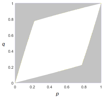
This bound has been generalized and improved in [10] and [11]. While tighter than the bound in Theorem 9, it still scales as when is small, hence not as tight as the bound in Corollary 1 when approaches zero. As an example, for two Bernoulli distributions with biases and , the white region in Fig. 1 indicates the collection of such that the bound in Corollary 1 is tighter than the bound in Theorem 10.
For differential entropy, the entropy difference can be upper-bounded in terms of the Wasserstein distance, as stated in the following result [12].
Theorem 11.
Let . If has a -regular density, meaning that
| (92) |
then
| (93) |
where is the Wasserstein distance with respect to the Euclidean distance of order .
Compared with the bound in (60), we see that (60) only requires the varentropy of to be finite, without other regularity conditions on . Moreover, the upper bound in (60) depends on only through , meaning that for a fixed , the upper bound is monotonically decreasing as gets closer to , which is sufficient to prove the upper semicontinuity of the entropy.
For the quadratic loss, the following result given by Wu [21] upper-bounds the variance difference in terms of the Wasserstein distance. It can be proved by writing and as and , and using the triangle inequality satisfied by the Wasserstein distance.
Theorem 12.
For and on with finite and ,
| (94) |
Compared with (62), the above upper bound only requires and to have finite second moments, while (62) requires to have a finite fourth moment. On the other hand, the upper bound in (62) depends on only through , hence monotonically decreasing as gets closer to , which is sufficient to prove the upper semicontinuity.
2.9 An information-theoretic application: mutual information upper bound
As an application of the entropy difference bounds derived in the previous subsections, we prove new upper bounds for mutual information by applying Corollary 1 and Corollary 5 to the log loss.
Corollary 12.
For jointly distributed random variables and that can be either discrete or continuous, let
| (95) |
be the range of variation of . Then from Corollary 5, we have
| (96) |
where is the Lautum information between and [22]. Moreover, from Corollary 1, we have
| (97) |
where may be regarded as a total variation information.
3 Application to frequentist learning
Having studied the continuity property of the generalized entropy as a functional of the underlying distribution, we now apply the results obtained in Section 2 to the excess risk analysis of learning methods, the central problem of statistical learning theory.
3.1 Excess risk of ERM algorithm
In the frequentist formulation of the statistical learning problem, there is a sample space , a fixed but unknown distribution on , and a hypothesis space . A loss function is chosen to evaluate the hypotheses in . For any hypothesis , its population risk is . is the minimum population risk that would be achieved among if were known. Neither nor is known however, due to the lack of knowledge of . What is available instead is a training dataset of size drawn i.i.d. from , with empirical distribution . As a natural choice, the empirical risk minimization (ERM) algorithm returns a hypothesis that minimizes the empirical risk among , and the minimum empirical risk is equal to . Since depends on , is a random variable. The entropy difference tells us how well the unknown minimum population risk can be approximated by the minimum empirical risk that is known in principle. The results in Section 2 enable us to upper-bound so as to evaluate the quality of this approximation.
More importantly, the upper-bounding techniques developed in Sections 2.1 to 2.6 provide us with a means to analyze the excess risk of the ERM algorithm, defined as the gap between the population risk of the algorithm-returned hypothesis and the minimum population risk:
| (104) |
where is a fresh sample from independent of , so that . Note that is a random variable, since depends on through . Writing as
| (105) |
and using the fact that all the entropy difference bounds in Sections 2.1 to 2.6 are based on Lemma 1, and the fact that every upper bound for obtained based on Lemma 1 also upper-bounds , we deduce the following result.
Lemma 3.
3.2 Finite sample space
When the sample space has a finite number of elements, we can make use of the entropy difference upper bounds in terms of total variation distance (Theorem 1) and KL divergence (Corollary 5). The resulting upper bounds for the excess risk hold virtually for any hypothesis space . For simplicity, we consider the case where the loss function takes values in .
Theorem 13.
If is finite and for all , then for any ,
| (107) |
and for any ,
| (108) |
Proof.
Remark. The upper bounds in Theorem 13 can be extended to the case where is countably infinite, using the results in [24, Lemma 8 and Theorem 3]. In addition, via Pinsker’s inequality, the upper bound in (108) can be used to bound , which complements the results in [24, Theorem 3] and [25, Lemma 3] on the convergence of empirical distribution in the total variation distance.
To evaluate the upper bounds in Theorem 13, consider the problem of binary classification, where with . Let be the space of all mappings from to , and . From (107), we get an upper bound for the expected excess risk of the ERM algorithm,
| (109) |
This bound is even better in prefactor than the bound given by the popular Rademacher complexity analysis, which is a consequence of the fact that the cardinality of the hypothesis class is when is finite [26].
3.3 Lipschitz-continuous loss function
When the loss function is Lipschitz-continuous in for all , where can be continuous-valued, we can use the bound in Theorem 5 in terms of the Wasserstein distance to bound the excess risk.
Theorem 14.
Let where and with . Suppose that is finite under the unknown distribution. Consider an action space with an arbitrary , and a function such that is -Lipschitz in with respect to the Euclidean distance for all . Then for the loss function ,
| (110) |
while for the loss function ,
| (111) |
where is an absolute constant.
Proof.
We first show that the Lipschitz continuity of in can be translated to the Lipschitz continuity of in . For any , and any ,
| (112) | ||||
| (113) | ||||
| (114) | ||||
| (115) |
where in (115) we used the fact that for . It implies that is -Lipschitz in for all . Since , it further implies that is -Lipschitz in for all . It follows from Lemma 3 and Theorem 5 that for ,
| (116) |
while for ,
| (117) |
The proof is completed with a result on the Wasserstein convergence of the empirical distribution [27, Theorem 3.1][28, Proposition 10], which states that for a distribution on with ,
| (118) |
where is some absolute constant. ∎
We see that the upper bound in Theorem 14 does not depend on the dimension of , and converges to zero as for any fixed dimension of ; however, the rate of convergence suffers from the curse of dimensionality in . An open question is whether there is a way to leverage the results in Section 2.4 to bounding the excess risk in terms of statistical distances between the distributions of when is drawn from and from . It may lead to tighter bounds when in Theorem 14 has additional regularities beyond being Lipschitz in . This question is partially addressed by looking into a statistical distance that compares the expected loss under distributions and , but at a worst hypothesis in , as discussed in the next subsection.
3.4 Learnability, typicality, and entropy continuity
The results in the two preceding subsections can be unified by considering the entropy difference bound via the -semidistance defined in (79). We have
| (119) |
which is essentially the uniform deviation of the empirical risk from the population risk with respect to . It follows from Lemma 3 and Theorem 7 that
| (120) |
This result recovers the classic upper bound on the excess risk of the ERM algorithm in terms of the uniform deviation [29].
The conditions on the convergence of the uniform deviation to zero,
| (121) |
have been well-studied in the mathematical statistics and statistical learning theory literature as a form of uniform law of large numbers [29, 26]. Recall that can also be defined with respect to the function class induced by as shown in (81), namely
| (122) |
The function class is called a Glivenko-Cantelli (GC) class if (121) holds for every distributon on , c.f. [30]. Further, the hypothesis space is said to be learnable with respect to if is a GC class. Theorem 13 and Theorem 14 each involves a special instance of the GC class that has virtually no restriction on : one with all measurable functions and a finite , such that
and the other with all bounded Lipschitz-continuous functions with a common Lipschitz constant, such that
In general, a GC class and the rate of convergence in (121) rely on the properties of both and . A well-known example of such a GC class is the class of indicator functions of a special collection of subsets of which has a finite Vapnik-Chervonenkis (VC) dimension [29]. For this class, with being the zero-one loss, and being the collection of subsets of with a finite VC dimension , explicitly depends on through
| (123) |
Conceptually, given and , we can also define the -typical set of elements in according to as in [30, Definition 4],
| (124) |
In words, a dataset is -typical if the empirical risks on it, uniformly for all hypotheses in , are close to the corresponding population risks. As a consequence of Theorem 7 in Section 2.6, the minimum empirical risk on this typical set can closely approximate the minimum population risk, as ; moreover, from (120), the ERM algorithm with an input drawn from this typical set will output a near-optimal hypothesis, as . For example, when and are such that is the set of measurable functions , the -typical set defined in (124) reduces to the one characterized by the total variation distance between and ,
| (125) |
which is proposed and used in [31]. When is finite, the above typical set is almost equivalent to the notion of strong typicality commonly used in information theory [7] [8, (10.106)] as shown in [31], and will include almost all elements in as . Theorem 13 can thus be understood from the viewpoint of strong typitcality as well, in that eventually almost every sequence has an empirical distribution close to . In general, the definition of applies to uncountably infinite as well. We then have the following connection among typicality, entropy continuity, and learnability: if is a GC class, then for any , as ,
| (126) |
by the definition in (124), which implies that
| (127) |
by Theorem 7, which further implies that
| (128) |
by Lemma 3. The rate of convergence will depend on and in general.
4 Application to Bayesian learning
Another application of the results in Section 2 to statistical learning is the analysis of the minimum excess risk in Bayesian learning. This problem is formulated and studied in detail in [5] using several different approaches. Here we give an overview of the analysis based on the entropy continuity presented in [5, Section 4].
4.1 Minimum excess risk in Bayesian learning
As an alternative to the frequentist formulation of the learning problem, Bayesian learning under a parametric generative model assumes that the data , with , is generated from a member of a parametrized family of probabilistic models , where the model parameter is an unknown random element in with a prior distribution . With a fresh sample , is observed, and the goal is to predict based on and . Formally, the joint distribution of the model parameter, the dataset and the fresh sample is
| (129) |
where for each . Given an action space and a loss function , the goal of Bayesian learning can be phrased as seeking a decision rule to make the expected loss small. In contrast to the frequentist learning, since the joint distribution is known, the search space here is all decision rules such that is defined, i.e. all measurable functions , without being restricted to a hypothesis space. The minimum achievable expected loss is called the Bayes risk in Bayesian learning:
| (130) |
which is essentially the generalized conditional entropy of given in view of the definition in (2). As shown by a data processing inequality for the Bayes risk [5, Lemma 1], decreases as the data size increases. The fundamental limit of the Bayes risk can be defined as the minimum expected loss when the model parameter is known:
| (131) |
The minimum excess risk (MER) in Bayesian learning is defined as the gap between the Bayes risk and its fundamental limit, which is the minimum achievable excess risk among all decision rules:
| (132) |
The MER is an algorithm-independent quantity. Its value and rate of convergence quantify the difficulty of the learning problem, which is due to the lack of knowledge of . It can serve as a formal definition of the minimum epistemic uncertainty, with serving as the definition of the aleatoric uncertainty, which have been only empirically studied so far [32, 33].
4.2 Method of analysis based on entropy continuity
In what follows, we outline the idea of how the upper bounds on entropy difference derived in Section 2 can be used to upper-bound the MER. We consider the predictive modeling framework, a.k.a. probabilistic discriminative model, where , with the probability transition kernel directly describing the predictive model of the quantity of interest given the observation. First, we have the following lemma that bounds the deviation of the posterior predictive distribution from the true predictive model , which is a simple consequence of the convexity of the statistical distance under consideration.
Lemma 4.
Let be a sample from the posterior distribution , such that and are conditionally i.i.d. given . Then for any -divergence or Wasserstein distance ,
| (133) |
where the expectations are taken over the conditioning variables according to the joint distribution of .
The main utility of Lemma 4 is that, whenever can be upper-bounded in terms of , we can invoke the fact that
| (134) |
as a consequence of the orthogonality principle in the MMSE estimation [34, 35, 36], so that the expected deviation can be bounded in terms of , the MMSE of estimating from . Lemma 4 and (134) give us a route to bounding the MER in terms of , provided we can bound the entropy difference in (132) in terms of . The latter problem is precisely the subject of Section 2.
4.3 Example: Bayesian logistic regression with zero-one loss
We give an example where the results in Section 2 can be applied to the analysis of Bayesian logistic regression with zero-one loss. Bayesian logistic regression is an instance under the predictive modeling framework, where , is assumed to be independent of , and the predictive model is specified by , with , , being the logistic sigmoid function, and being the feature vector of the observation.
For the zero-one loss, whenever is discrete, we have
| (135) | ||||
| (136) | ||||
| (137) | ||||
| (138) |
where (137) follows from Theorem 1, and (138) follows from Lemma 4. With the predictive model specified above, as , we know that is -Lipschitz in , hence
| (139) |
Consequently, the MER with respect to zero-one loss satisfies
| (140) | ||||
| (141) | ||||
| (142) | ||||
| (143) |
where the last step is due to (134) and the assumption that and are independent.
This result explicitly shows that the MER in logistic regression depends on how well we can estimate the model parameters from data, as it is dominated by , the MMSE of estimating from . A closed-form expression for this MMSE may not exist; nevertheless, any upper bound on it that is nonasymptotic in will translate to a nonasymptotic upper bound on the MER. Moreover, this result explicitly shows how the model uncertainty due to the estimation error of the model parameters translates to the MER under the zero-one loss, which represents the minimum epistemic uncertainty, and how it then contributes to the minimum overall prediction uncertainty, which is the sum of the MER and the aleatoric uncertainty . It thus provides a theoretical guidance on uncertainty quantification in Bayesian learning, which is an increasingly important direction of research with wide range of applications.
5 Application to inference and learning with distribution shift
Based on Lemma 1, we have developed a number of approaches to bounding the difference of the generalized unconditional entropy in Section 2. We also studied the applications of the results in both frequentist learning and Bayesian learning in the two preceding sections. The idea behind Lemma 1 can be extended to bounding the difference of the generalized conditional entropy defined in (2). In this section, we work out this extension to derive performance bounds for Bayes decision making under a mismatched distribution. The results can be applied to analyzing the excess risk in learning by first projecting the empirical distribution to a predefined family of distributions and then using the projection as a surrogate of the data-generating distribution for decision making.
5.1 Bounds on conditional entropy difference
Consider the Bayes decision-making problem under which the generalized conditional entropy is defined as in (2). Let and be two joint distributions on . Given an action space and a loss function , let and be the Bayes decision rules with respect to under and respectively, such that and Note that and are the optimal actions that achieve the generalized unconditional entropy of and respectively. Then, in the same spirit of Lemma 1, we have the following result for the difference between generalized conditional entropy.
Lemma 5.
Let and be two joint distributions on . Then the difference between the generalized conditional entropy with respect to under and satisfy
| (144) |
and
| (145) |
With Lemma 5, all the results developed in Sections 2.1 to 2.6 on the entropy difference can be extended to bounds for the conditional entropy difference. For example, the results in Sections 2.1, 2.2 and 2.3 can be extended by replacing and by and respectively, in both the conditions and the bounds, and by replacing the statistical distances between and by distances between and . In view of Theorem 4 in Section 2.4, the statistical distances between and can even be replaced by distances between and , or between and . In view of the results in Section 2.5, we can also bound the conditional entropy difference by the Wasserstein distance between and if or is Lipschitz in . Moreover, we can define an -semidistance between and as
| (146) |
and use it to bound the conditional entropy difference, similar to the results in Section 2.6.
As an illustrative example, suppose the loss function for all . Then
| (147) | ||||
| (148) | ||||
| (149) |
where (147) is due to Lemma 5; (148) is due to (34); and (149) follows from the chain rule of KL divergence. Not only serving as an upper bound for the conditional entropy difference, the result also implies that when both and are small, can closely approximate . As mentioned above, other methods developed in Section 2 can be extended for this purpose as well, and may provide even tighter performance guarantees.
In the special case where and share the same marginal distribution of , the decision rule defined above preserves its optimality under this new , and we have the following alternative bounds due to the representation of the conditional entropy via the unconditional entropy in (3) and Lemma 1.
Lemma 6.
Under and , let and . Then
| (150) |
and
| (151) |
With Lemma 6, the results developed in Sections 2.1 to 2.6 on unconditional entropy difference can be directly applied to bounding the conditional entropy difference, by bounding the integrands in (150) and (151).
The bounds for conditional entropy difference obtained in Lemma 5 or Lemma 6 combined with the techniques developed in Section 2 can provide performance guarantees for decision making with distribution shift: the performance of a decision rule under a new distribution , represented by , may be approximated in terms of its performance under the original distribution where it is optimally designed, represented by . As illustrated by the preceding example for , the simple upper bound for the right-hand side of (147) given in (149) is an analogue of the result in [37, Theorem 1] on binary classification with distribution shift, and is an extension of it to general Bayesian inference problems.
5.2 Excess risk bounds via entropy difference
Besides comparing against , it is also of interest to study the gap between and , which amounts to the excess risk incurred by using under distribution rather than using the optimal decision rule . The following result, in the same spirit of Lemma 3, shows that the excess risk can be upper-bounded in terms of the previously developed upper bounds for the conditional entropy difference or .
Theorem 15.
Proof.
To show (152), we can write the entropy difference as
| (154) |
The claim then follows from the fact that any upper bound for obtained based on Lemma 5 also upper-bounds .
Next we prove (153). Adopting the same definitions of and as in Lemma 6, we have
| (155) | ||||
| (156) | ||||
| (157) |
where (156) uses the fact that remains as a Bayes decision rule under the joint distribution ; and the last step is due to (151) in Lemma 6.
As an example, we can use Theorem 15 to bound the excess risk in estimating from a noisy observation when the prior distribution of is wrongly specified. For instance, when has a prior distribution and with independent of , if the prior distribution of is assumed to be , then the mismatched Bayes estimator with respect to the quadratic loss is instead of the true Bayes estimator [38]. The following corollary bounds the excess risk of using a mismatched Bayes estimator in a more general setting.
Corollary 13.
Suppose has a prior distribution , and with some function and noise independent of . Let be the Bayes estimator with respect to the quadratic loss when the prior distribution of is assumed to be while is assumed to have the same functional dependence on and . Then
| (158) |
Proof.
This result is a slight variation of (152), but we follow the same line of its proof:
| (159) | ||||
| (160) | ||||
| (161) | ||||
| (162) |
where (161) follows from the same argument as in the proof of Theorem 3; and the last step uses the fact that and , which follows from the definition of the divergence and the fact that and are identical and only depend on the distribution of , as a consequence of the assumed form of . ∎
Theorem 15 can also be applied to statistical learning problems where the learned decision rule is optimally designed under a data-dependent distribution . Combined with the results in Section 2, it can provide excess risk upper bounds in terms of the statistical distances between and the data-generating distribution . We give an example in the next subsection.
5.3 Excess risk in learning by projecting to exponential family
We now consider a procedure for supervised learning that is different from both the frequentist learning and the Bayesian learning discussed in the previous sections. To precisely describe it, we need the following definitions and properties of exponential family distributions. A parametrized family of distributions on is an exponential family if each element can be written as for some , with as a potential function, as the log partition function, and as a density on . For a distribution on which may not belong to , its projection to , defined as , is given by with a that satisfies
| (163) |
Similarly, given a dataset drawn i.i.d. from , the projection of its empirical distribution to , defined as the solution to the maximum-likelihood estimation , is given by with a that satisfies
| (164) |
Define the convex conjugate of as for any that can be written as for some . When is minimal, meaning that and are different for any , it is known from convex duality [39] that and implicitly defined above can be explicitly written as and . Figure 2 illustrates the above defined quantities.

With the above definitions, the learning procedure under consideration can be described as follows: given a dataset drawn i.i.d. from , first project its empirical distribution to a predefined exponential family on to obtain , then the learned decision rule for predicting based on a fresh observation is taken as the Bayes decision rule that is optimal under . The following result based on Theorem 15 provides upper bounds for its expected excess risk.
Corollary 14.
For the learning procedure described above, under the assumptions that is minimal and that the loss function takes values in , the expected excess risk of using as the learned decision rule under the data-generating distribution satisfies
| (165) |
where the expectations are taken over either or with as the underlying distribution.
Proof.
To make use of Theorem 15, we first bound the entropy difference. For any realization of the dataset ,
| (166) |
where the first inequality is due to Lemma 5 and the assumption that as used in the proof of Theorem 1, while the second inequality is due to the triangle inequality satisfied by the total variation distance. Further,
| (167) | ||||
| (168) | ||||
| (169) | ||||
| (170) |
where (167) uses the Pinsker’s inequality; (168) uses the property of the exponential family distributions; (169) uses the fact that and the Cauchy-Schwarz inequality; and (170) uses (163) and (164) as well as the assumption that is minimal so that . It then follows from (152) in Theorem 15 that
| (171) |
almost surely for . The claim follows by taking expectations on both sides of the above inequality over and applying Jensen’s inequality on the right-hand side. ∎
Corollary 14 clearly shows that the excess risk for learning by projecting the empirical distribution to an exponential family consists of two parts: the approximation error, represented by the first term on the right-hand side of (165), and the estimation error, represented by the second term. The approximation error depends on the total variation distance from the data-generating distribution to the exponential family and does not depend on the data size. The estimation error on the other hand vanishes as grows whenever and are continuous, which is due to the fact that almost surely as .
The learning procedure considered above can be extended to the cases where the family of distributions is not predefined, but dependent on the empirical distribution , and where the distribution under which the learned decision rule is optimally designed is found by other criteria. An example is the recently proposed maximum conditional entropy framework of learning [2], where is a set of distributions centered at , and is chosen to be an element of with the maximum generalized conditional entropy with respect to some loss function. A special case of this framework with moment-matching conditions to construct and with the log loss may be interpreted as projecting the empirical conditional distribution to an exponential family of conditional distributions associated with a generalized linear model. More generally, the minimax approach to statistical learning where the goal is to find a decision rule that minimizes the worst-case expected loss in , c.f. [2, 6] and the reference therein, is equivalent to the maximum conditional entropy approach under regularity conditions [2]. Whether Theorem 15, especially (153) can be leveraged to analyze the excess risk in the maximum conditional entropy framework of learning would be an interesting research problem.
6 Possible improvements and extensions
In this work, we have derived upper and lower bounds for the difference of the generalized entropy between two distributions in terms of various statistical distances, and applied the results to the excess risk analysis in three major learning problems. In this section we discuss possible improvements and extensions of this work.
- •
Improvement of the entropy difference bound. The majority of the entropy difference bounds obtained in Section 2 are based on Lemma 1. Only in Section 2.7 we took a different route by considering an exact representation of the entropy difference in terms of a Bregman divergence between the distributions. There is another exact representation of the entropy difference, which can be viewed as a refinement of Lemma 1:
(172) The slack of Lemma 1 is clearly seen as the nonnegative , which can be thought of an -specific divergence between and [1]. A possible way to improve the results obtained based on Lemma 1 is thus to evaluate or lower-bound .
- •
Applying Theorem 4 to learning problems. As shown in Section 2.4, Theorem 4 can potentially provide much tighter entropy difference bounds. The reason is that the loss is real-valued, with a one-dimensional distribution, whereas the data distribution or can be high-dimensional. The difficulty to apply this improvement to frequentist learning problems is that, the empirical loss is a function of non-i.i.d. quantities, as the learned hypothesis depends on the training data. It is thus hard to characterize the resulting distribution of the empirical loss. But this problem can be an interesting future direction of research.
- •
Continuity of other general definitions of entropy. The generalized entropy considered in this work is a function of probability distribution on a sample space. This definition could be further generalized to functions of other quantities of interest, e.g. to the von Neumann entropy (a.k.a. quantum entropy) as a function of the density matrix. Such generalization may also be carried out in a decision-making framework [40]. It is therefore of interest to study if the continuity property of other generalized entropies can be useful for analyzing excess risks of the related decision-making or optimization problems.
Appendix
Appendix A Proof of Lemma 2
The Donsker-Varadhan theorem states that
| (173) |
It implies that for any and any ,
| (174) |
From the assumption that for all and the definition for , we have
| (175) | ||||
| (176) |
From the definition for , we have
| (177) |
which proves (25).
The Donsker-Varadhan theorem also implies that for any and any ,
| (178) |
From the assumption that for all and the definition for , we have
| (179) | ||||
| (180) |
From the definition for , we have
| (181) |
which proves (27).
The assumption that is strictly convex over and implies that its Legendre dual is strictly increasing over and . In addition, the fact that is convex over implies that it is continuous over . Together these imply that is strictly increasing and continuous over , and . It follows that . The same argument can be used to show that if is strictly convex over and , then .
Acknowledgment
The author would like to thank Prof. Maxim Raginsky, Prof. Yihong Wu, and Jaeho Lee for helpful discussions. The author is also thankful to the area editor and anonymous reviewers of the IEEE Transactions on Information Theory, their comments greatly improved the quality of the paper.
References
- [1] P. D. Grünwald and A. P. Dawid, “Game theory, maximum entropy, minimum discrepancy and robust Bayesian decision theory,” Ann. Statist., vol. 32, no. 4, pp. 1367–1433, 2004.
- [2] F. Farnia and D. Tse, “A minimax approach to supervised learning,” in Conference on Neural Information Processing Systems, 2016.
- [3] P. Harremoës, “Information topologies with applications,” in Entropy, Search, Complexity, I. Csiszár, G. O. H. Katona, G. Tardos, and G. Wiener, Eds. Springer Berlin Heidelberg, 2007.
- [4] A. Xu, “Continuity of generalized entropy,” in IEEE International Symposium on Information Theory, 2020.
- [5] A. Xu and M. Raginsky, “Minimum excess risk in Bayesian learning,” arXiv preprint arXiv:2012.14868, 2020.
- [6] J. Lee and M. Raginsky, “Minimax statistical learning with Wasserstein distances,” in Conference on Neural Information Processing Systems, 2018.
- [7] I. Csiszár and J. Körner, Information Theory: Coding Theorems for Discrete Memoryless Systems. Academic Press, 1981.
- [8] T. Cover and J. Thomas, Elements of Information Theory, 2nd ed. New York: Wiley, 2006.
- [9] Z. Zhang, “Estimating mutual information via Kolmogorov distance,” IEEE Transactions on Information Theory, vol. 53, no. 9, pp. 3280–3282, 2007.
- [10] S. Ho and R. W. Yeung, “The interplay between entropy and variational distance,” IEEE Transactions on Information Theory, vol. 56, no. 12, pp. 5906–5929, 2010.
- [11] I. Sason, “Entropy bounds for discrete random variables via maximal coupling,” IEEE Transactions on Information Theory, vol. 59, no. 11, pp. 7118–7131, 2013.
- [12] Y. Polyanskiy and Y. Wu, “Wasserstein continuity of entropy and outer bounds for interference channels,” IEEE Transactions on Information Theory, vol. 62, no. 7, 2016.
- [13] Y. Wu and S. Verdú, “Functional properties of minimum mean-square error and mutual information,” IEEE Transactions on Information Theory, vol. 58, no. 3, pp. 1289–1301, 2012.
- [14] S. Boucheron, G. Lugosi, and P. Massart, Concentration Inequalities: A nonasymptotic theory of independence. Oxford University Press, 2013.
- [15] J. Jiao, Y. Han, and T. Weissman, “Dependence measures bounding the exploration bias for general measurements,” in IEEE International Symposium on Information Theory (ISIT), 2017.
- [16] Y. Bu, S. Zou, and V. V. Veeravalli, “Tightening mutual information based bounds on generalization error,” in IEEE International Symposium on Information Theory (ISIT), 2019.
- [17] I. Sason and S. Verdú, “ -divergence inequalities,” IEEE Transactions on Information Theory, vol. 62, no. 11, pp. 5973–6006, 2016.
- [18] Y. Wu, “Lecture notes on information-theoretic methods in high-dimensional statistics,” University of Illinois/Yale University, 2016-2020.
- [19] I. Kontoyiannis and S. Verdú, “Optimal lossless compression: Source varentropy and dispersion,” in IEEE International Symposium on Information Theory, July 2013, pp. 1739–1743.
- [20] L. Bregman, “The relaxation method of finding the common point of convex sets and its application to the solution of problems in convex programming,” USSR Computational Mathematics and Mathematical Physics, vol. 7, no. 3, pp. 200–217, 1967.
- [21] Y. Wu, personal communication, 2019.
- [22] D. P. Palomar and S. Verdú, “Lautum information,” IEEE Transactions on Information Theory, vol. 54, no. 3, pp. 964–975, March 2008.
- [23] D. Berend and A. Kontorovich, “A sharp estimate of the binomial mean absolute deviation with applications,” Statistics and Probability Letters,, vol. 83, pp. 1254–1259, 2013.
- [24] ——, “On the convergence of the empirical distribution,” arXiv:1205.6711, 2012.
- [25] L. Devroye, “The equivalence of weak, strong and complete convergence in for kernel density estimates,” vol. 11, no. 3, pp. 896–904, 09 1983.
- [26] S. Shalev-Shwartz and S. Ben-David, Understanding Machine Learning: From Theory to Algorithms. Cambridge University Press, 2014.
- [27] J. Lei, “Convergence and concentration of empirical measures under Wasserstein distance in unbounded functional spaces,” Bernoulli, vol. 26, no. 1, pp. 767–798, 02 2020.
- [28] J. Weed and F. Bach, “Sharp asymptotic and finite-sample rates of convergence of empirical measures in Wasserstein distance,” Bernoulli, vol. 25, no. 4A, pp. 2620–2648, 11 2019.
- [29] L. Devroye, L. Györfi, and G. Lugosi, A Probabilistic Theory of Pattern Recognition. Springer, 1996.
- [30] M. Raginsky, “Empirical processes, typical sequences, and coordinated actions in standard Borel spaces,” IEEE Transactions on Information Theory, vol. 59, no. 3, pp. 1288–1301, March 2013.
- [31] P. W. Cuff, H. H. Permuter, and T. M. Cover, “Coordination capacity,” IEEE Transactions on Information Theory, vol. 56, no. 9, pp. 4181–4206, 2010.
- [32] A. Kendall and Y. Gal, “What uncertainties do we need in Bayesian deep learning for computer vision?” in Conference on Neural Information Processing Systems, 2017.
- [33] E. Hüllermeier and W. Waegeman, “Aleatoric and epistemic uncertainty in machine learning: A tutorial introduction,” ArXiv 1910.09457, 2019.
- [34] J. Liu, P. Cuff, and S. Verdú, “On alpha-decodability and alpha-likelihood decoder,” in The 55th Ann. Allerton Conf. Comm. Control Comput., 2017.
- [35] A. Bhatt, J.-T. Huang, Y.-H. Kim, J. J. Ryu, and P. Sen, “Variations on a theme by Liu, Cuff, and Verdú: The power of posterior sampling,” in IEEE Information Theory Workshop, 2018.
- [36] B. Hajek, Random processes for engineers. Cambridge University Press, 2015.
- [37] S. Ben-David, J. Blitzer, K. Crammer, A. Kulesza, F. Pereira, and J. W. Vaughan, “A theory of learning from different domains,” Machine Learning, vol. 79, no. 1, pp. 151–175, May 2010.
- [38] S. Verdú, “Mismatched estimation and relative entropy,” IEEE Transactions on Information Theory, vol. 56, no. 8, pp. 3712–3720, 2010.
- [39] M. J. Wainwright and M. I. Jordan, “Graphical models, exponential families, and variational inference,” Foundations and Trends in Machine Learning, vol. 1, no. 1–2, pp. 1–305, 2008.
- [40] P. Harremoës, “Divergence and sufficiency for convex optimization,” Entropy, vol. 19, no. 5, 2017.