The APOGEE Library of Infrared SSP Templates (A-LIST):
High-Resolution Simple Stellar Population Spectral Models in the -Band
Abstract
Integrated light spectroscopy from galaxies can be used to study the stellar populations that cannot be resolved into individual stars. This analysis relies on stellar population synthesis (SPS) techniques to study the formation history and structure of galaxies. However, the spectral templates available for SPS are limited, especially in the near-infrared. We present A-LIST (APOGEE Library of Infrared SSP Templates), a new set of high-resolution, near-IR SSP spectral templates spanning a wide range of ages (2–12 Gyr), metallicities () and abundances (). This set of SSP templates is the highest resolution () available in the near infrared, and the first such based on an empirical stellar library. Our models are generated using spectra of 300,000 stars spread across the Milky Way, with a wide range of metallicities and abundances, from the APOGEE survey. We show that our model spectra provide accurate fits to M31 globular cluster spectra taken with APOGEE, with best-fit metallicities agreeing with those of previous estimates to within 0.1 dex. We also compare these model spectra to lower-resolution E-MILES models and demonstrate that we recover the ages of these models to within 1.5 Gyr. This library is available in https://github.com/aishashok/ALIST-library.
Keywords:
infrared: stars - infrared: galaxies - stars: evolution - galaxies: evolution - galaxies: stellar content - Astrophysics - Astrophysics of GalaxiesI Introduction
Observing, modeling and analysis of individual stars in the visible spectrum has formed the foundation for our understanding of stellar evolution. In turn, our understanding of galaxies today: their star formation rates, evolutionary histories, and stellar masses, is almost entirely based on our knowledge of stellar evolution. Resolved stellar populations allow us to measure the colors, luminosities and compositions of individual stars, provides useful information about the history and structure of their galaxies. Resolved population studies are possible only in the Milky Way (Ruiz-Lara et al. 2020, e.g.,) as well as nearby spiral and dwarf galaxies (Williams et al. 2009; Weisz et al. 2011; Lewis et al. 2015, e.g,). In more distant galaxies, integrated spectroscopy has been an important method to study their unresolved stellar content. The integrated spectrum of a population reflects its star formation histories and chemical enrichment. Using spectral lines to study the physical properties of stars and stellar populations has been known as early as 1960s and has improved ever since (Spinrad & Taylor 1971; Mould 1978; Chavez et al. 1996; Parikh et al. 2019).
Earlier work studying galaxy stellar populations focused primarily on line index measurements (Worthey et al. 1994; Trager et al. 2000; Thomas et al. 2003; Gallazzi et al. 2005; Schiavon 2007; Caldwell et al. 2011, e.g.) in the optical part of the spectrum as well as in the near-infrared (Vazdekis et al. 1996; Böker et al. 1999; Cenarro et al. 2001; Förster Schreiber et al. 2003; Cenarro et al. 2009; MacArthur et al. 2010; Vazdekis et al. 2010; Onken et al. 2014; Riffel et al. 2019, NIR; e.g.). In recent years, full spectral fitting of integrated light spectra to model spectra has opened a new window to study in detail the physical, chemical and evolutionary phases of galaxy stellar populations (Pérez et al. 2013; Pace et al. 2019; Boardman et al. 2020, e.g.). Some of the most widely used spectral fitting software for this technique are FIREFLY (Wilkinson et al. 2017), STECKMAP (Ocvirk et al. 2006), VESPA (Tojeiro 2007), pPXF (Cappellari et al. 2009), ULySS(Koleva et al. 2009), STARLIGHT (Cid Fernandes et al. 2011), and Pipe3D (Sánchez et al. 2016a; Sánchez et al. 2016b). Most of the pixel fitting stellar population studies to date have used optical spectroscopy to derive information about galaxy formation histories (Heavens et al. 2004; McDermid et al. 2015, e.g.). .The NIR part of the spectrum offers some advantages over the optical due to the reduced affects of dust extinction and the sensitivity to cool stars. Over the past decade or so, a large number of studies have studied stellar populations using the NIR (Silva et al. 2008; Cesetti et al. 2009; Mármol-Queraltó et al. 2008; Sakari et al. 2016; La Barbera et al. 2016; La Barbera et al. 2017; Röck et al. 2017; Baldwin et al. 2018; Dahmer-Hahn et al. 2018; Martins et al. 2019; Coelho et al. 2020, e.g.).
These direct spectral fitting techniques use the Stellar Population Synthesis (SPS) technique, where spectra are modeled with a combination of synthetic populations to disentangle their age and chemical abundances. The foundation of this method is the Simple Stellar Population (SSP) model where all the stars are coeval and share the same chemical composition. Creating model stellar populations has progressed greatly in the last three decades from the trial and error technique (Tinsley 1968; Bruzual & Charlot 2003; Maraston 2005; Vazdekis et al. 2010; Röck et al. 2016; Conroy et al. 2018, e.g.).
Given the wide range of information we want to gain from SPS fitting: the star formation history and rate, initial mass function, chemical enrichment, metallicity etc., creating optimal and flexible SSP models remains a major challenge in modern evolutionary studies. There are 2 ways these SSPs can be constructed (i) Fuel Consumption Based approach (Maraston 2005, e.g.) and (ii) The Isochrone Synthesis approach which we use in this paper. With the Isochrone Synthesis Method, we can construct the SSPs as having an Initial Mass Function along an isochrone and a stellar library (Bruzual & Charlot 2003, e.g.).
The theoretical stellar libraries (Gustafsson et al. 2008, e.g. MARCS library,) are generated using a desired range of parameters that cannot be obtained from observations at any range of wavelength, while the empirical libraries (Prugniel et al. 2007; Gonneau et al. 2020, e.g.,ELODIE library, X-shooter Library (R10,000)) are based on real observational data. Large spectroscopic surveys like APOGEE (Majewski et al. 2017), GALAH (De Silva et al. 2015), etc. can provide us with tens of thousands of Milky Way star properties that can be used to model stellar populations. To study the stellar absorption features in old populations, empirical libraries are preferred (Maraston et al. 2009; Vazdekis et al. 2016), while for young and bright populations, theoretical libraries are preferred (Maraston 2005; Leitherer et al. 2014). Martins et al. 2019; Coelho et al. 2020 explain in detail how these two types of libraries are used.
The models we present here address two specific deficits in existing SPS models. First, most models don’t consider varying abundances, and abundances are typically still derived using spectral indices rather than pixel fitting to SPS models (Schiavon et al. 2012; Janz et al. 2016; Johnston et al. 2020, e.g.). Second, there are no SPS models based on empirical stellar libraries in the NIR available at high spectral resolution. The only high spectral resolution NIR models (R20,000) are the version of the Maraston & Strömbäck 2011 models created using the MARCS theoretical stellar spectra library. See Baldwin et al. 2018 for how these models compare with other available NIR models and data. Existing models based on empirical stellar libraries available in the NIR (Bruzual & Charlot 2003; Maraston & Strömbäck 2011; Meneses-Goytia et al. 2015; Vazdekis et al. 2016; Röck et al. 2016; Conroy et al. 2018) use the Pickles 1998 stellar library and the IRTF library (Cushing et al. 2005; Rayner et al. 2009). These are both low spectral resolution, with the IRTF library having the higher resolution of R2000.
This spectral resolution is lower than that of many current and planned spectrographs: Gemini/NIFS (McGregor et al. 2003), VLT/SINFONI (Eisenhauer et al. 2003), GEMINI/GNIRS (Elias et al. 2006), ESO/KMOS (Wisnioski et al. 2015), VLT/MOONS (Cirasuolo & MOONS Consortium 2016), Keck/MOSFIRE (Steidel et al. 2017), JWST/NIRSPEC (Ygouf et al. 2017). For data taken from these spectrographs, using the current available models based on empirical stellar libraries requires degrading the data resolution and losing information while modeling.
In this paper, we present A-LIST (APOGEE Library of Infrared SSP Templates), a new library of high resolution SSP spectral models generated using a new empirical stellar library based on Apache Point Observatory Galaxy Evolution Experiment (Majewski et al. 2017, APOGEE;) data from the Sloan Digital Sky Survey-IV (Blanton et al. 2017, SDSS-IV;). The SSP models range in age, [M/H] and [/M]. This is a first of its kind spectral library in the H-band region having a high spectral resolution (R 22500). This library can be used to model, for example, (i) any near IR integrated light spectra having a spectral resolution greater than the current available SSP models; (ii) enhancement and kinematics of globular clusters (GCs) and/or early-type galaxies; and (iii) nearby galaxy data (M31, M33) available from APOGEE (Zasowski et al. 2013, Beaton et al. in prep). Because APOGEE spectra are not precisely flux calibrated, A-LIST spectral models are primarily useful for integrated light spectroscopic studies.

We discuss the required ingredients and our selections in Section II. In Section III, we discuss how we generate the Simple Stellar Population models in detail. In Section IV, we present our spectral models. Section V, we present our validation of these models by reproducing properties of M31 GCs and comparisons to previously studied models. The summary along with future work is described in Section VI.
II Simple Stellar Population Model Ingredients
In this section, we outline the main ingredients, including the isochrone sets (Section II.1) and the stellar library (Section II.2).
II.1 Stellar Evolution and Isochrones
One of the main ingredients to generate an SSP model is an isochrone or a set of stellar evolutionary tracks.
For our models, we use two different isochrone sets:
- •
PARSEC isochrones: the latest Padova isochrones and stellar evolutionary tracks (Bressan et al. 2012; Chen et al. 2014; Chen et al. 2015; Tang et al. 2014; Marigo et al. 2017; Pastorelli et al. 2019) are computed spanning a wide range in ages and metallicities. The library of isochrones includes stars with initial masses M⊙, , and metallicities . The PARSEC stellar tracks range in initial metal content from 0.0001 to 0.06, with 15 values in the grid, and range in mass from 0.1 to 350 M⊙ with 120 different mass values for each metallicity (Marigo et al. 2017).
- •
MIST evolutionary tracks: MESA Isochrones and Stellar Tracks (Dotter 2016; Choi et al. 2016; Paxton et al. 2011; Paxton et al. 2013; Paxton et al. 2015, MIST;) is another set of evolutionary track models that has an extensive range of mass ( M⊙), age (), and metallicity (). The evolutionary tracks used to generate the isochrones range in mass from 0.1 to 300 M⊙ with 100 models at different masses, and in [Fe/H] from -2.0 to +0.5 with 0.25 dex spacing (Choi et al. 2016). We use the models with , i.e., those models which do not include any stellar rotation parameters in them.
Both sets of models use interpolation of the evolutionary tracks to create isochrones at a given age and metallicity. The list of ages and metallicities used in our models is given in Section IV.
One of the main differences between the PARSEC and the MIST isochrones is the method used to interpolate the TP-AGB evolutionary tracks. This results in the C-rich AGB stars in the MIST isochrones starting at a later point in their evolutionary track compared to those of PARSEC (Marigo et al. 2017; Choi et al. 2016). The C-rich AGB stars in MIST isochrones are hotter than those in PARSEC mainly because the MIST isochrones use molecular opacities derived for O-rich mixtures (Marigo et al. 2017). For a detailed description of how these two isochrone sets differ, see Marigo et al. 2017; Choi et al. 2016; Cignoni et al. 2019.
Figure 1 shows the two isochrone sets plotted over the empirical library of APOGEE stars (Section II.2) colored by metallicity, with Padova isochrones on the left and MIST on the right.
The isochrones available in Padova and MIST have solar –abundances. To obtain the most accurate isochrones for our models with non-solar –abundance (), we use the -enhanced metallicity equation (from Salaris & Cassisi 2005, chapter 8) for the solar-scaled isochrones with the metallicity as:
| (1) |
where is the solar scaled metallicity and gives the effective metallicity of the isochrones used to account for the –enhancement. We note that we use this value only for selecting the isochrones of appropriate metallicity for a model with desired and solar-scaled .
II.2 Empirical Stellar Library

The second main ingredient needed to generate an SSP model is the empirical stellar spectral library. One strength of A-LIST is the availability of several hundred thousand stellar spectra from the APOGEE survey that can be used as an empirical library. APOGEE (Majewski et al. 2017) is a spectroscopic survey of the Milky Way and a component of the Sloan Digital Sky Survey (Eisenstein et al. 2011; Blanton et al. 2017, SDSS-III and -IV;)
APOGEE samples stars that span across the Milky Way’s bulge, disk and halo with a wide range of stellar parameters and abundances (Zasowski et al. 2017; Zasowski et al. 2013). The data are collected with two 300-fiber spectrographs (Wilson et al. 2019) at the 2.5-meter Sloan Foundation Telescope at the Apache Point Observatory in New Mexico (Gunn et al. 2006) and at the 2.5-meter duPont Telescope at Las Campanas Observatory in Chile (Bowen & Vaughan 1973). The wavelength range of APOGEE spectra is 1.51–1.70m, which is divided across three chips: “blue” chip at m, “green” chip at m, and “red” chip at m, with gaps between the detectors at m and m). APOGEE’s average resolving power () is 22,500 based on a direct-measured FWHM of 0.7Å, with 10-20% variations seen across the wavelength and fiber (Nidever et al. 2015, see Section 6.2).
We use an internal APOGEE data release that is an increment from the latest public data release (Ahumada et al. 2019, DR16;), which has new stars added from the observing period through November 2019. The incremental release applies the same DR16 pipeline (Jönsson et al. 2020) to the additional data, which include both new targets and repeat visits for stars in DR16.
APOGEE data are first processed by the APOGEE data reduction pipeline (Nidever et al. 2015). The stellar parameters and elemental abundances are computed by the APOGEE Stellar Parameters and Chemical Abundances Pipeline (García Pérez et al. 2016, ASPCAP;). For our empirical library, we use the calibrated ASPCAP parameters to select cool dwarfs and giants, and the uncalibrated parameters (“FPARAM”) to select hot dwarfs ( K). See Jönsson et al. 2020 and Holtzman et al. 2018 for a description of APOGEE’s calibration procedures and data products.
To obtain a set of APOGEE stars with reliable ASPCAP measurements and high SNR we make the following cuts:
- 1.
SNR: We remove all stars with median per pixel .
When creating the median spectrum for a given stellar parameter bin (Section III.2), we only consider pixels with an individual , computed with the stellar error spectra.
- 2.
VSCATTER: We remove all stars that have a radial velocity scatter greater than 1.5 km s-1. This cut reduces the impact of spectroscopic binary stars on our sample.
- 3.
VERR: We remove all stars that have a radial velocity error greater than 3 km s-1. This limit ensures that the selected stars are properly corrected to the rest frame.
- 4.
ASPCAPFLAG bitmask: We remove all stars that are marked as STARBAD (bit 23), TEFFBAD (bit 16), LOGGBAD (bit 17), or COLORTEWARN (bit 9).
- 5.
STARFLAG bitmask: We remove all stars that are marked BRIGHTNEIGHBOR (bit 2), VERYBRIGHTNEIGHBOR (bit 3), PERSISTHIGH (bit 9), PERSISTMED (bit 10), PERSISTLOW (bit 11), SUSPECTRVCOMBINATION (bit 16), or SUSPECTBROADLINES (bit 17).
Based on these cuts, we select 293,220 stars from the incremental DR16 data. In this paper, we use [M/H] as our solar-scaled metallicity based on its definition in Section 6.5.1 of Majewski et al. 2017. The left panel of Figure 2 shows an HR Diagram of the APOGEE stellar sample that we use as our empirical stellar library. The right panel of Figure 2 shows the [M/H] and [/M] distribution of the APOGEE stars. Both the plots are colored by the number of stars in each bin. The axes on these two plots define the limits within which our models are generated.
We found it necessary to renormalize some of the pseudo-continuum normalized APOGEE spectra, due to systematic offsets in the pseudo-continuum determination, before combining the spectra. For all stars whose median normalized flux is greater than 1.04, and stars that show wing-like features (especially at the chip edges), we renormalize the spectra by fitting a 3rd, 4th, and 3rd order polynomial to the blue, green, and red chips of the spectra, respectively. An example of this is shown in Figure 3. Here the blue line shows the APOGEE pseudo-continuum-normalized spectrum. We see wide wing-like features, most prominently here at the edges of the blue and green detectors. With renormalization, we bring the median flux of the spectrum closer to 1 (as shown in orange).
II.3 Other data used in this paper
Additional data adopted in this paper includes stellar ages, used for calculating offsets between the isochrones and the APOGEE stars (Section III.3). We use ages (’AGE_LOWESS’) from the astroNN Value Added Catalog (Leung & Bovy 2019; Mackereth et al. 2019)11 1 https://www.sdss.org/dr16/data_access/value-added-catalogs/?vac_id=the-astronn-catalog-of-abundances,-distances,-and-ages-for-apogee-dr16-stars, derived using a neural network trained on the stellar spectra from DR14 (Jönsson et al. 2018).
We also use a set of M31 GC spectra, which were observed as part of an APOGEE ancillary project (Zasowski et al. 2013) as well as a custom analysis of these data performed by Sakari et al. 2016, for validation of our models (Section V.2). These spectra were made using the APOGEE apVisit files, with an approach nearly identical to the automated APOGEE pipeline that produces the combined apStar files22 2 https://www.sdss.org/dr16/irspec/spectral_combination/. The difference is that we did not use the measured visit-level RVs when combining the visit spectra, because we found that some of these RVs were discrepant from the cluster mean; our combined GC spectra are thus in the observed frame, not the stellar rest frame.
III Generating Simple Stellar Population Models
In this section, we describe the steps in making a SSP spectral model along with how we use each ingredient. We adopt the Isochrone Synthesis method based on equation (1) from Section 2 of Conroy 2013:
| (2) |
where is the spectrum of a star with an initial stellar mass . The isochrones with an initial mass function (M) relate the Teff– distributions to an age () and chemical composition (Z). The model spectrum represents the integration (from a lower limit , usually considered to be the hydrogen burning limit, to an upper limit imposed by stellar evolution) of all the individual spectra from APOGEE along the isochrone, weighted by the fractional luminosity at a given Teff and from the isochrone in the HR diagram.
The isochrones for our SSP generation span a range in age, [M/H], and [/M] as described in Section IV.
III.1 Generating Synthetic Stellar Populations
Using an isochrone at a given [M/H] and [/M], we generate an SSP using the Kroupa 2001 IMF with an initial mass of . Based on tests we ran using different initial masses (Beerman et al. 2012, e.g.,) from – , was selected as the minimum one needed to ensure that multiple SSPs generated from the same isochrone did not differ in the total number of stars or total luminosity by more than 1%, due to stochastic sampling.
Our synthetic SSPs are generated using a package called PyPopStar (Hosek Jr et al. 2020). This is a python package that generates synthetic single-age, single-metallicity population. We generate the synthetic SSP using our isochrones (age, metallicity and mass) and the initial mass of . The conditions to generate the SSP are:
- •
Isochrone object: Isochrones from Padova or MIST (Section II.1).
- •
Initial mass = M⊙
- •
IMF = Kroupa 2001
- •
Stellar Multiplicity: Defines the properties of multiple systems in a population based on the IMF. This function defines how the stellar masses influence the synthetic population. We use the ’MultiplicityUnresolved()’ with parameters defined in Lu et al. 2013.
- •
Synthetic star clusters: Using the isochrone object, IMF and the initial mass, we use the resolved star cluster function ’ResolvedCluster()’ which interpolates the isochrone points within the mass limits to generate the synthetic population.
Each synthetic SSP generated is characterized by an age, [M/H], and [/M] and describes the Teff, , and luminosity of stars at a given mass of M⊙.
III.2 Parameter Grid for SSP Spectral Model Generation
To construct our SSP spectral models (referred to as A-LIST models from here on), we need to obtain spectra that represent the simulated stars in a 4D parameter space (Teff, , [M/H], and [/M]) for each age, [M/H], and [/M] isochrone. For this, we define 4D bins that span the range of Teff, , [M/H], and [/M] needed for the simulated stars. We define bin sizes such that the stars in each bin have on average 1% difference between their normalized spectra and the bin’s median spectrum:
- 1.
Effective temperature (Teff): The full width of the bin Teff = 50 K for 3000 K Teff 5000 K and the full width of the bin Teff = 150 K for 5000 K Teff 10000 K. We use a larger bin size for the hotter stars to increase the number of stars per bin (and the number of occupied bins), after confirming that the spectral variations within the bin are still within 1%.
- 2.
Surface gravity (): dex for .
- 3.
Metallicity ([M/H]): dex for and dex for .
- 4.
-abundance ([/M]): We define our [/M] bins based on the Teff of the stars. For all stars having Teff 5700K and , dex. For hotter temperatures Teff 5700K (i.e., the main sequence stars), there are insufficient –enhanced stars in our sample. However, because these hot stars have weaker lines, we found that the spectral variations at a given [M/H], log g and Teff bin across all are still within 1% at these temperatures. Therefore, for these hot temperature bins we select all stars regardless of –enhancement in a given [M/H], Teff and log g bin.
III.3 Surface Gravity Offset
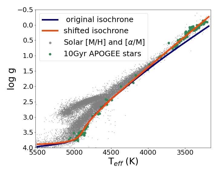
When matching both the Padova and MIST isochrones with the empirical stellar library, we find that there are offsets in surface gravity and temperature along the upper part of the RGB. Similar offsets along the upper RGB have been seen in previous work (Serenelli et al. 2017; Durbin et al. 2020, e.g.,). The uncertainties in the APOGEE are too small to account for these offsets, and the size of the offset varies for the different isochrone sets. Hence, to account for this difference, we shift the isochrone by a function defined by the offset between the stars and the isochrone in the RGB phase of evolution.
For each isochrone corresponding to an age, [M/H] and [/M], we select the APOGEE stars having the same [M/H] and [/M]. Based on the astroNN ages for APOGEE (Section II.3), we further select stars that are the closest 10% in age to the isochrone. We then calculate the offset in the RGB evolutionary phase of the isochrone () from the mean of the APOGEE stars in each temperature bin (Section III.2). A 3rd order polynomial is fit to this offset and the isochrones are shifted to match the APOGEE stars.
Figure 4 shows an example of this process. A 10 Gyr, solar [M/H], solar [/M] isochrone (blue line) is plotted over the solar [M/H], solar [/M] APOGEE stars (39,000 stars; shown as small grey points). The 10% of APOGEE stars with astroNN ages closest to 10 Gyr in the RGB evolutionary phase are shown as big green points (170 stars). The isochrone shifted in to match these points is shown as an orange line. For the shift shown in Figure 4, the standard deviation of the difference between the shifted and unshifted spectra is just 0.14%, while the maximum difference in the spectra is 1%.
III.4 Incorporating the APOGEE Spectral Library
To obtain the integrated-light model spectrum of an SSP, the synthetic SSPs generated from the isochrones and the APOGEE stars are both binned in the 4D cube (Section III.2). Each bin is assigned a weight based on the fractional luminosity it contains, from the total synthetic SSP. In addition, each bin is assigned a median spectrum calculated from all of the APOGEE stars in that bin. Then, the final A-LIST model SSP is obtained by summing the median spectra from all the bins, each scaled by its luminosity weight determined from the binned synthetic SSP.
IV Description of A-LIST Models
In this section, we describe the integrated near-infrared SSP model spectra created from APOGEE and synthetic SSPs. A-LIST contains SSP spectral models based on Padova isochrones and MIST isochrones, available at a range of ages, metallicities, and –abundances:
- 1.
Age (Gyr): 2.0, 3.0, 4.0, 5.0, 6.0, 7.0, 8.0, 9.0, 10.0, 11.0, 12.0
- 2.
Metallicity ([M/H]): -2.2, -1.9, -1.6, -1.3, -1.0, -0.8, -0.6, -0.4, -0.2, 0.0, +0.2, +0.4
- 3.
–abundances ([/M]): -0.2, -0.1, 0.0, +0.1, +0.2, +0.3, +0.4
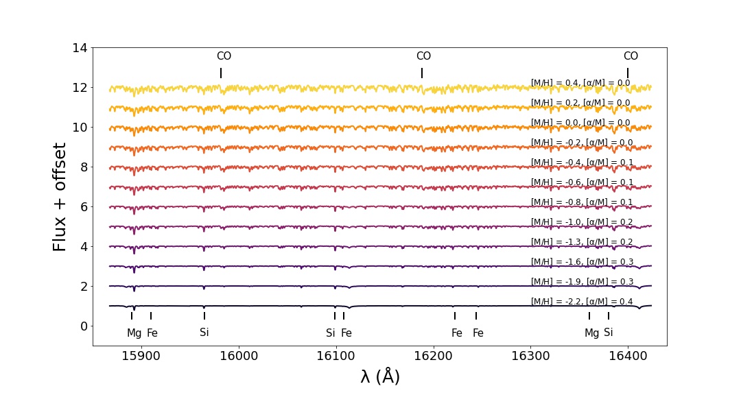
Figure 5 shows examples of 10 Gyr old, Padova–based A-LIST spectral models varying in [M/H] and [/M] across the full range of [M/H]. The abundance change in the models is reflected in many of the absorption lines, strengthening from metal poor to metal rich, e.g., in the Fe lines visible at 15900 Å. Figure 6(a) shows examples of 10 Gyr old, Padova-based A-LIST spectral models with and different [/M]. An example of how models change with [/M] can be seen at the CO bandheads at 15990 & 16180 Å, as well as in the Mg line at 16365 Å. In all cases these -element lines increase in strength from -poor to -rich models.
Figure 6(b) shows the mean equivalent width (EW) of lines of different elements for each of the high fractional luminosity A-LIST models (0.5; see Section IV.1.1) shown in Figure 6(a). We calculate the EW of non-blended absorption lines in the model spectra corresponding to Fe, Al, and Mn (non- elements) and to Mg and Si (-elements). Each of the points shown in Figure 6(b) is the mean value of all the individual elemental EWs normalized to their element’s [/M]=0 values. The total number of lines represented in this plot are 74 for Fe, 8 for Mn, 5 for Al, 13 for Mg, and 18 for Si. We see an increase in the -element EWs (solid lines), in contrast to the non- element EWs (dashed lines). Indeed, the non- EWs decrease at higher [/M], as expected with scaled-solar [M/H] held constant.
For each model, we also provide a spectrum that characterizes the standard deviation of the individual stellar spectra in each 4D bin used to create that model. The standard deviation of the spectra are measured at each spectral pixel in each 4D bin, and then these individual bin standard deviation spectra are added together using the same weights as the model spectra. This “variance” spectrum has a typical value of 1% across all ages, [M/H], and [/M]. However, as we show in the next section, the dominant uncertainties in our model spectra are due to a lack of APOGEE stellar spectra for some models in log g–Teff bins, which are not reflected in the provided variance spectrum.
IV.1 Metrics for Assessing the Accuracy of A-LIST Models
One simple method to validate the A-LIST models is to compare the differences between the models and an ideal synthetic stellar population model. In this section, we assume the synthetic SSPs to fully represent a stellar population of a given age, [M/H], and [/M]. The differences observed are due to either a lack of available stars in our empirical stellar library or our binning methods. We discuss the similarities between A-LIST models and the synthetic SSPs in terms of the luminosity recovered (Section IV.1.1) and the average Teff (Section IV.1.2). We also discuss the variation of the average metallicity and -abundance of A-LIST models from the defined bin center (Section IV.1.3).
IV.1.1 Fraction of the Synthetic SSP Luminosity Represented in A-LIST Models
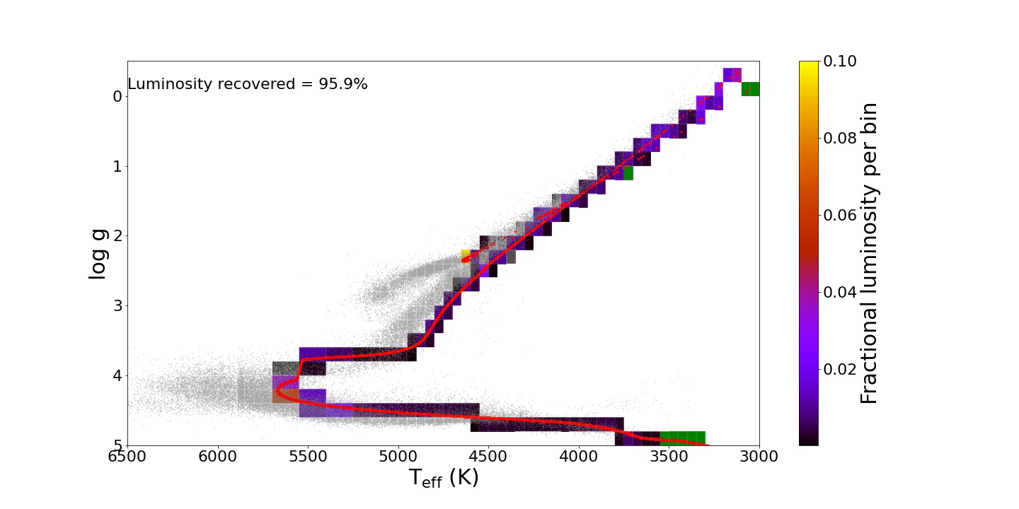
One important aspect of the A-LIST spectral models is how much of the total synthetic SSP luminosity is represented. Figure 7 shows a HR Diagram that describes how we compute the fractional luminosity from the synthetic SSP for one A-LIST model (10 Gyr, solar [M/H], solar [/M]). The APOGEE stars with the same [M/H] and [/M] are shown as black points. The synthetic SSP is shown as red points. From this synthetic SSP we calculate the fraction of light in each of our spectral bins (Section III.2), which is indicated by the color of the bin. Bins that have a non-zero fraction of luminosity but no APOGEE stars in them — i.e., bins that are not represented in the final A-LIST model spectrum — are colored green. There are 8000 stars at solar [M/H] and solar [/M] (Figure 2(b)), enabling the high fractional luminosity here (0.97).
Figure 8(a) shows the fractional luminosity of each 10 Gyr A-LIST spectral model as a function of [M/H] and [/M]. In general, the highest fractional luminosities coincide with the most-populated parts of chemical abundance space in the APOGEE sample. In Section V.4 we discuss in detail how the fractional luminosity captured by the A-LIST models impacts the model properties and fits. We demonstrate there that the models with luminosity fraction below 0.32 are less reliable, and thus in Figure 8(a) we highlight the reliable models with a white dashed outline.
IV.1.2 Average temperature of A-LIST Models
Figure 8(b) shows the difference in the luminosity-weighted average Teff for 10 Gyr A-LIST models, as a function of [M/H] and [/M], between the Padova-based synthetic SSPs and corresponding A-LIST models. The large negative differences are due to a lack of cool (3500 K), low surface gravity stars in our APOGEE sample at particular metallicity and combinations (e.g., at and , where K). The large positive differences are due to a lack of hot (7000 K) main sequence stars; these are mostly in our lower metallicity models (e.g., at and , where K). In Section V.4 we assess how the change in luminosity-weighted average Teff impacts the model properties.
IV.1.3 Variation in Metallicity and -abundance
In Section III.2 we define the [M/H] and [/M] bins in our hypercube based on the desired model grid values. These bin values are assigned to the generated spectral models, assuming that the mean [M/H] and [/M] values of stars in the bin is the same as that of the bin center (e.g., in the [M/H] bin with bin-edges , we assume the mean ).
However, due to the non-uniform distribution of APOGEE stars across our bins, our mean [M/H] and [/M] are sometimes offset from the bin centers as shown in Figure 8(c). The red points indicate the mean [M/H] and [/M] values for 10 Gyr Padova-based A-LIST models. These values are obtained by calculating the average [M/H] and [/M] weighted by the fractional luminosity of all the APOGEE stars with K (i.e., all stars that are binned by [/M]). The bin centers are shown by the inner red lines. For example, in the and bin, we select stars with -1.1 [M/H] -0.9. Although the mean based on the bin edges, the actual mean , based on the stars available in the bin. The average absolute offset from the input [M/H] is 0.013 for all models with luminosity fraction above 0.32 (including those inside the dashed line in Figure 8(c)), while for [/M] this average absolute offset is 0.018.
IV.2 Difference Between Padova and MIST Based Models
A-LIST consists of spectral models generated using two different isochrone sets: Padova and MIST (Section II.1). Figure 9 shows a comparison between 10 Gyr, solar [M/H], solar [/M] MIST-based (shown in blue) and Padova-based (shown in fuchsia) A-LIST model spectra. The maximum difference is 3%, and the standard deviation of the difference is 1%.
The difference between Padova-based and MIST-based model spectra arises from the differences in the isochrones, primarily from the cooler temperature bins (briefly explained in Section II.1). For example, in Figure 9, the TP-AGB stars in the MIST-based population have K, and in the Padova–based one, they have K. This 100 K difference leads to deeper absorption lines in the Padova models, with a maximum difference of 3%. In Section V.2 we show that while overall both models recover the metallicities and -abundances of globular clusters, these model differences lead to small differences in measurements for individual clusters. We note that, consistent with the TP-AGB star difference discussed above, typically the Padova models have luminosity weighted effective temperatures that are 100K hotter than the MIST models with the same population parameters.
Figure 10 shows the standard deviation in the difference between the 10 Gyr MIST–based and Padova–based A-LIST models models as a function of [M/H] and [/M]. We see that the difference in the models for the most populated parts of the chemical abundance space is 1.5% of the normalized flux. The bins with larger deviations (1.5%) correspond to the least-populated parts of chemical abundance space of the APOGEE stars (like very metal-poor, solar- bins and metal-rich, -rich bins), which also correspond to regions lying outside the white “high reliability” contour (Section V.4).

V SPECTRAL MODEL VALIDATION
In this section, we validate A-LIST models by recovering the kinematics, [M/H], and [/M] of M31 GCs and by comparing our A-LIST spectral library to the lower resolution E-MILES (Vazdekis et al. 2016) library.
V.1 Fitting procedure
We use the Penalized Pixel-Fitting method (Cappellari et al. 2009; Cappellari 2017, pPXF;), a full-spectrum fitting code that calculates stellar kinematics and stellar population parameters from absorption-line spectra using a maximum penalized likelihood approach. We compute velocities, dispersions, and stellar population parameters for the GCs using A-LIST as templates, and to compare the age and [M/H] of our high resolution models with a low resolution spectral library.
V.2 M31 GCs
GCs are not perfect SSPs (Gratton et al. 2012, e.g.,), but are very close to being so; hence, they are useful for validating our A-LIST models by recovering the properties of previously studied clusters observed by APOGEE (Section II.3). We select 32 GCs with 10 SNR 150 (Sakari et al. 2016, 7 of which were studied in).
To determine the properties of the GCs, we fit each of our A-LIST models one-at-a-time to the GCs over the wavelength range of the green and red detectors (i.e., Å). We do not use the blue detector due to the presence of high persistence in many spectra (Majewski et al. 2017, see Section 3.4 of). We take the likelihood-weighted average for age, [M/H], and [/M] from the three fits with smallest reduced values. We use all A-LIST models with age 6 Gyr to reduce the time needed to run the code. The uncertainties on these fits are calculated in two different ways: for radial velocity and the velocity dispersion, the systematic uncertainty on the best fit model is determined by a simple bootstrapping for . For [M/H] and [/M], we calculate the uncertainty using the relative of the best fit model relative to other models. More specifically, we derive our uncertainties in [M/H] and [/M] by using a limit corresponding to a 1 uncertainty, deriving both lower and upper limits.
Table 1 shows the radial velocity, velocity dispersion, [M/H], [/M], and age of the M31 GCs determined using the A-LIST library, both Padova–based and MIST–based, along with the uncertainties.
Figure 11 shows an example of a high SNR GC spectrum (B127-G185, SNR = 150) with its best fit A-LIST Padova–based model spectrum, for a small section of the wavelength range ( Å). The GC spectrum is first masked for bad sky lines as well as in regions where the error on the flux is high. The residuals are very small (standard deviation )
Figure 12 compares our best-fit values from the A-LIST models with literature values. Due to a lack of available [/M] literature measurements for our M31 GCs, we use [Mg/Fe] derived from the line indices in Schiavon et al. 2012 to compare with A-LIST [/M]. The literature comparison for the other parameters are obtained from Strader et al. 2011 for velocity dispersion and radial velocities and from Caldwell et al. 2011 for [Fe/H]. We also include radial velocities, metallicity, and [/Fe] estimates for these GCs from Sakari et al. 2016.
The dynamical and chemical properties recovered from the A-LIST models agree well with these previous literature values (Table 2). For Padova-based (MIST-based values in parentheses) we find a median offset (literature – A-LIST) of 0.09 (0.04) in [M/H] and 0.02 (0.02) in [/M], while the median absolute deviation is 0.1 (0.08) in [M/H] and 0.04 (0.04) in [/M]. These median absolute deviations are comparable to or smaller than the size of the literature errors on these quantities.
Overall, we find that the MIST-based model metallicities match more closely those of Caldwell et al. 2011, while the Padova-based models give somewhat lower metallicities. This lower metallicity is consistent with the deeper lines seen for the same population parameters in the Padova-based templates relative to the MIST-based templates, due to the cooler AGB stars and luminosity-weighted . A Spearman rank correlation between our A-LIST [/M] values and the [Mg/Fe] of Schiavon et al. 2012 gives a correlation coefficient of 0.64 and a p-value of 1.37x10⁻⁴, suggesting a very significant correlation.
| MIST–based SSP | Padova–based SSP | ||||||||||
|---|---|---|---|---|---|---|---|---|---|---|---|
| Globular cluster | SNR | RV | [M/H] | [/M] | Age | RV | [M/H] | [/M] | Age | ||
| (km s-1) | (km s-1) | (Gyr) | (km s-1) | (km s-1) | (Gyr) | ||||||
| B006-G058 | 25 | -235.90.3 | 12.90.4 | -0.5 | 0.2 | 10.3 | -235.90.3 | 13.00.2 | -0.6 | 0.3 | 10.3 |
| B012-G064 | 23 | -362.1 1.9 | 13.72.3 | -1.6 | 0.1 | 10.3 | -361.61.9 | 17.42.7 | -1.8 | 0.1 | 10.3 |
| B023-G078 | 180 | -440.30.4 | 28.50.4 | -0.5 | 0.1 | 6.7 | -442.30.6 | 29.50.4 | -0.5 | 0.1 | 6.3 |
| B025-G084 | 10 | -202.72.6 | 11.82.9 | -1.5 | 0.1 | 8.3 | -202.20.8 | 8.80.2 | -0.9 | 0.2 | 8.4 |
| B045-G108 | 17 | -426.10.5 | 11.40.5 | -0.9 | 0.2 | 10.6 | -426.30.3 | 10.90.3 | -1.0 | 0.2 | 10.6 |
| B063-G124 | 34 | -304.10.4 | 18.20.5 | -1.0 | 0.2 | 10.3 | -304.10.3 | 18.60.3 | -1.0 | 0.2 | 8.3 |
| B068-G130 | 23 | -321.60.3 | 9.10.3 | -0.2 | 0.2 | 9.7 | -321.60.3 | 9.50.3 | -0.2 | 0.2 | 9.7 |
| B088-G150 | 32 | -482.41.5 | 9.81.5 | -1.6 | 0.0 | 8.5 | -484.7.01.4 | 16.21.3 | -1.6 | 0.1 | 8.8 |
| B103-G165 | 98 | -367.6 0.3 | 17.30.3 | -0.4 | 0.3 | 11.3 | -367.30.2 | 17.30.2 | -0.6 | 0.2 | 10.7 |
| B107-G169 | 47 | -332.80.8 | 16.31.1 | -1.0 | 0.1 | 11.3 | -333.20.8 | 15.91.1 | -1.2 | 0.2 | 11.3 |
| B109-G170 | 23 | -620.30.2 | 7.70.3 | -0.3 | 0.3 | 10.1 | -620.30.2 | 7.50.3 | -0.3 | 0.3 | 10.0 |
| B112-G174 | 20 | -276.50.2 | 10.20.3 | -0.5 | 0.2 | 9.0 | -276.70.2 | 11.50.3 | -0.2 | 0.1 | 10.3 |
| B115-G177 | 36 | -599.70.3 | 13.10.3 | -0.3 | 0.2 | 10.8 | -599.70.2 | 13.10.2 | -0.2 | 0.2 | 10.6 |
| B127-G185 | 151 | -527.80.4 | 23.40.4 | -0.6 | 0.2 | 10.1 | -527.80.2 | 23.20.3 | -0.7 | 0.2 | 10.3 |
| B128-G187 | 15 | -382.40.8 | 11.50.9 | -0.6 | 0.3 | 10.9 | -382.30.8 | 11.70.9 | -0.6 | 0.2 | 11.1 |
| B129 | 59 | -413.70.5 | 18.20.6 | -1.0 | 0.2 | 10.4 | -43.70.3 | 18.20.3 | -0.8 | 0.2 | 9.6 |
| B131-G189 | 105 | -466.40.6 | 22.70.6 | -0.5 | 0.2 | 9.3 | -466.30.4 | 22.80.6 | -0.7 | 0.2 | 9.1 |
| B151-G205 | 125 | -324.50.5 | 22.10.4 | -0.6 | 0.1 | 9.6 | -342.30.3 | 22.30.2 | -0.7 | 0.2 | 10.3 |
| B153 | 50 | -246.90.3 | 11.90.4 | -0.3 | 0.2 | 10.3 | -246.90.2 | 11.90.2 | -0.3 | 0.3 | 10.8 |
| B171-G222 | 72 | -269.10.3 | 14.60.3 | -0.4 | 0.2 | 10.1 | -269.10.2 | 14.50.2 | -0.4 | 0.2 | 9.8 |
| B180-G231 | 12 | -198.90.3 | 9.10.9 | -1.0 | 0.2 | 9.0 | -198.90.7 | 9.20.9 | -1.0 | 0.1 | 9.0 |
| B190-G241 | 10 | -88.80.3 | 6.81.7 | -1.3 | 0.2 | 10.6 | -88.30.4 | 7.11.8 | -1.1 | 0.1 | 10.4 |
| B193-G244 | 29 | -62.10.3 | 17.20.3 | -0.2 | 0.2 | 8.8 | -62.10.2 | 16.80.1 | -0.2 | 0.3 | 8.6 |
| B206-G257 | 58 | -194.30.6 | 16.20.7 | -1.1 | 0.2 | 9.7 | -194.20.7 | 16.90.1 | -1.1 | 0.2 | 9.7 |
| B213-G264 | 14 | -572.10.9 | 8.70.2 | -0.7 | 0.1 | 9.9 | -572.10.3 | 8.90.6 | -0.9 | 0.1 | 10.2 |
| B313-G036 | 19 | -420.33.2 | 10.93.9 | -0.8 | 0.1 | 10.0 | -426.20.8 | 7.81.7 | -1.2 | 0.1 | 11.00 |
| B373-G305 | 86 | -220.10.3 | 12.40.3 | -0.5 | 0.3 | 9.9 | -220.50.2 | 13.10.8 | -0.7 | 0.3 | 9.8 |
| B386-G322 | 48 | -393.80.5 | 12.80.9 | -1.1 | 0.2 | 9.3 | -393.50.9 | 14.31.5 | -1.3 | 0.3 | 9.3 |
| B403-G348 | 40 | -265.60.5 | 9.90.6 | -0.9 | 0.1 | 10.4 | -265.50.3 | 9.70.4 | -0.9 | 0.0 | 10.2 |
| B407-G352 | 49 | -296.20.5 | 9.20.4 | -0.6 | 0.1 | 11.4 | -296.70.2 | 9.70.9 | -0.7 | 0.2 | 11.4 |
| B472-D064 | 55 | -115.80.5 | 22.81.6 | -1.1 | 0.1 | 9.5 | -116.70.3 | 22.50.2 | -1.2 | 0.1 | 9.5 |
Note. — The selection of GCs (32 shown here from 185 available) is based on available literature values as well as based on physical pPXF fits with reasonable values. We eliminate those GCs that have a very noisy spectra and/or have a continuum issue in their chips.
| RV | [M/H] | [/M] | ||||||
|---|---|---|---|---|---|---|---|---|
| (km s-1) | (km s-1) | (dex) | dex | |||||
| MIST–based | Padova–based | MIST–based | Padova–based | MIST–based | Padova–based | MIST–based | Padova–based | |
| median offset | -1.5 | -1.3 | 0.4 | 0.2 | 0.04 | 0.09 | 0.02 | 0.02 |
| median absolute deviation | 0.74 | 0.66 | 1.55 | 1.53 | 0.08 | 0.1 | 0.04 | 0.04 |
V.3 E-MILES comparison
We also compare our library to the popular E-MILES (Vazdekis et al. 2016) models for the same age and metallicity. The lower metallicity E-MILES models (i.e, ) are composite spectra generated by extrapolating the available SSP spectra from MIUSCAT (Vazdekis et al. 2012) and the IRTF library (Vazdekis et al. 2012, Section 2 of). Since our spectral resolution is much higher than that of E-MILES, we convolve the A-LIST spectra with a Gaussian kernel to reduce our resolution to match that of the E-MILES spectra. Using the pPXF code and the same fitting method as Section V.2, we calculate the likelihood-weighted average values for the age and metallicity. The uncertainty or the “pseudo-error” on the A-LIST best fit model is calculated using the same method as explained for the metallicity and –abundance in Section V.2. Since these models do not have any errors on them, the pseudo-error is scaled by a normalized error (scatter between best fit model and the data) on the best fit model.
Figure 13 shows the computed age and [M/H] from the best-fit reduced resolution Padova-based (orange) and MIST-based (blue) A-LIST templates (with ) fitted to E-MILES models at a range of ages (2–12 Gyr) and metallicities (-0.7, -0.4, -0.2, 0.0, and +0.2 dex).
Our models show close correspondence in both age and metallicity to lower resolution E-MILES models. For Padova-based (MIST-based values in parentheses) we find a median offset (E-MILES – A-LIST) of 0.7 (0.5) Gyr in age and 0.06 (0.06) dex in metallicity, while the median absolute deviation is 1.48 (0.88) Gyr in age and 0.09 (0.17) in metallicity. For the age comparison, MIST-based fits better match the E-MILES models, with both smaller offsets and a smaller median absolute deviation than the Padova-based fits. For metallicities the two models provide quite similar offsets.
Figure 14 shows comparisons between the best-fit Padova-based A-LIST templates (at the E-MILES resolution; fuchsia) and E-MILES models (blue) using templates with solar- and a range of ages and metallicities. The differences between the best-fit Padova-based A-LIST and E-MILES models are shown in green.

. The differences in the best-fit values between the Padova-based and MIST-based for these models are small. The fits (Section V.3) are performed over the full APOGEE wavelength range, but only a small section is shown here to highlight the similarity.
V.4 Model spectra quality test based on globular cluster fitting
Two major factors affecting the reliability of the A-LIST model spectra, in terms of how representative a spectrum is of its nominal SSP, are the fraction of recovered luminosity (Section IV.1.1) and the difference in the luminosity-weighted average Teff between the synthetic population and the model spectrum (; Section IV.1.2). To understand how these affect our spectral models, we conduct tests in which we generate sets of modified A-LIST templates from a high luminosity fraction, low model to simulate lower luminosity fractions and higher values (e.g., Figure 7). To test the effects of lower fractional luminosities, we remove the bins that have the largest contributions to the total SSP luminosity. To test the effects of having a non-zero , we remove the hottest and coldest Teff bins.
For the recovered luminosity fraction test, we generate these degraded template sets for the best-fitting SSP to three of our high-SNR GCs (B127-G185, B151-G205 and B103-G165, with SNRs of 150, 127 and 103, respectively). We perform the same fitting as in Section V.1 and observe the relation between the of the fits and the fractional luminosity. As the fractional luminosity decreases (i.e., the more bins we remove from the HRD), the values of the fits increase, as expected. Based on this increase in , we define a cut-off fractional luminosity for the A-LIST models of 0.32, below which we caution the models may not provide reliable results. This value of 0.32 is selected based on where we see an increase in the reduced of 0.25 relative to the best fit, highest luminosity fraction model.
We note that while this fraction may seem fairly low, many of the spectral bins in the HRD used in constructing our A-LIST models have spectra similar to each other, thus enabling accurate spectral models even at lower fractional luminosities.
We use two approaches for the test. In one, we generate degraded templates to fit the same three high-SNR GCs as above. To test how our models fare at different ages and metallicities, we also create mock data at younger ages and different metallicities by generating noisy data from our models assuming a S/N of 50. We then fit both the GCs and the mock data to the degraded models using the same fitting method in Section V.1 and observe the relation between the of the fits and . By progressively removing the hottest and coldest Teff bins and then fitting the degraded templates to GC spectra or mock data created from our original models, we find that a of K and a of K correspond to a .
To summarize, we recommend using only models with luminosity fraction 0.32 and K; models meeting these requirements have been highlighted in Figure 8. Our “best” models (by these metrics) lie in the region of chemical space where the majority of MW stars reside (the right panel of Figure 2). The quality of our models decreases in bins with few stars available (e.g., regions outside the white line in Figure 8(a)).
VI Summary
In this paper, we present A-LIST: a new spectral library of high resolution, near-infrared integrated-light simple stellar population spectral templates that can be used to compute the properties of complex stellar populations having multiple populations with different ages, [M/H], and [/M]. This library is generated using the isochrone synthesis method with Padova and MIST isochrones and a Kroupa 2001 IMF. We use an empirical stellar library with 300,000 stars from the APOGEE survey, which has a spectral resolution of 22,500 and a wavelength range of 15100 to 17000 Å. The empirical stellar library provides enough APOGEE spectra to generate SSP spectral models representing as much as 99% of the luminosity of the SSPs, with lower fractional luminosities found in regions of [M/H] and [/M] space that are not well represented in the Milky Way.
Our validation tests demonstrate that our models give fitting results consistent in both age and metallicity with previous measurements and with lower resolution models . First, we fit the A-LIST models to APOGEE spectra of M31 GCs and find metallicities consistent with previous measurements by Caldwell et al. 2011 and Sakari et al. 2016, with a median offset of 0.1 dex. The [/M] measurements of our M31 GCs are also well-correlated with previously estimated values. Second, we fit our A-LIST library to E-MILES models at a range of ages and metallicities and find a good agreement with the E-MILES models in the best-fit ages (with a median absolute deviation 1.5 Gyr) as well as the best-fit metallicities (with a median absolute deviation 0.17 dex).
We also use the fits to the globular clusters and to generated mock data to better understand where our models are most reliable. We find that models with fractional luminosity 0.32, and with the difference in temperature between the synthetic population and our corresponding model of K, provide high quality fits to the spectra. We recommend these thresholds in using our model spectra.
Our models are publicly available at
https://github.com/aishashok/ALIST-library. We expect they will be useful in analyzing medium- and high-resolution -band integrated light spectroscopy of galaxies and star clusters.
We would like to thank Ricardo Schiavon and Nelson Caldwell for providing us with the [Mg/Fe] abundances of M31 GCs. We would also like to thank the anonymous referee whose comments significantly improved this paper. Work on this project by AA, GZ, and AS was supported by NSF grant AST-1911129. Additional work was supported by NSF PHY-REU Award #1659494. DAGH acknowledges support from the State Research Agency (AEI) of the Spanish Ministry of Science, Innovation and Universities (MCIU) and the European Regional Development Fund (FEDER) under grant AYA2017-88254-P.
Funding for the Sloan Digital Sky Survey IV has been provided by the Alfred P. Sloan Foundation, the U.S. Department of Energy Office of Science, and the Participating Institutions. SDSS-IV acknowledges support and resources from the Center for High-Performance Computing at the University of Utah. The SDSS web site is www.sdss.org.
SDSS-IV is managed by the Astrophysical Research Consortium for the Participating Institutions of the SDSS Collaboration including the Brazilian Participation Group, the Carnegie Institution for Science, Carnegie Mellon University, the Chilean Participation Group, the French Participation Group, Harvard-Smithsonian Center for Astrophysics, Instituto de Astrofísica de Canarias, The Johns Hopkins University, Kavli Institute for the Physics and Mathematics of the Universe (IPMU) / University of Tokyo, the Korean Participation Group, Lawrence Berkeley National Laboratory, Leibniz Institut für Astrophysik Potsdam (AIP), Max-Planck-Institut für Astronomie (MPIA Heidelberg), Max-Planck-Institut für Astrophysik (MPA Garching), Max-Planck-Institut für Extraterrestrische Physik (MPE), National Astronomical Observatories of China, New Mexico State University, New York University, University of Notre Dame, Observatário Nacional / MCTI, The Ohio State University, Pennsylvania State University, Shanghai Astronomical Observatory, United Kingdom Participation Group,Universidad Nacional Autónoma de México, University of Arizona, University of Colorado Boulder, University of Oxford, University of Portsmouth, University of Utah, University of Virginia, University of Washington, University of Wisconsin, Vanderbilt University, and Yale University.
References
- Ahumada et al. (2019) Ahumada, R., Allende Prieto, C., Almeida, A., et al. 2019, arXiv e-prints, arXiv:1912.02905. https://arxiv.org/abs/1912.02905
- Baldwin et al. (2018) Baldwin, C., McDermid, R. M., Kuntschner, H., Maraston, C., & Conroy, C. 2018, MNRAS, 473, 4698, doi: 10.1093/mnras/stx2502
- Beerman et al. (2012) Beerman, L. C., Johnson, L. C., Fouesneau, M., et al. 2012, ApJ, 760, 104, doi: 10.1088/0004-637X/760/2/104
- Blanton et al. (2017) Blanton, M. R., Bershady, M. A., Abolfathi, B., et al. 2017, AJ, 154, 28, doi: 10.3847/1538-3881/aa7567
- Boardman et al. (2020) Boardman, N., Zasowski, G., Seth, A., et al. 2020, MNRAS, 491, 3672, doi: 10.1093/mnras/stz3126
- Böker et al. (1999) Böker, T., van der Marel, R. P., & Vacca, W. D. 1999, AJ, 118, 831, doi: 10.1086/300985
- Bowen & Vaughan (1973) Bowen, I. S., & Vaughan, A. H. 1973, Appl. Opt., 12, 1430, doi: 10.1364/AO.12.001430
- Bressan et al. (2012) Bressan, A., Marigo, P., Girardi, L., et al. 2012, MNRAS, 427, 127, doi: 10.1111/j.1365-2966.2012.21948.x
- Bruzual & Charlot (2003) Bruzual, G., & Charlot, S. 2003, Monthly Notices of the Royal Astronomical Society, 344, 1000, doi: 10.1046/j.1365-8711.2003.06897.x
- Caldwell et al. (2011) Caldwell, N., Schiavon, R., Morrison, H., Rose, J. A., & Harding, P. 2011, AJ, 141, 61, doi: 10.1088/0004-6256/141/2/61
- Cappellari (2017) Cappellari, M. 2017, MNRAS, 466, 798, doi: 10.1093/mnras/stw3020
- Cappellari et al. (2009) Cappellari, M., di Serego Alighieri, S., Cimatti, A., et al. 2009, ApJ, 704, L34, doi: 10.1088/0004-637X/704/1/L34
- Cenarro et al. (2001) Cenarro, A. J., Cardiel, N., Gorgas, J., et al. 2001, MNRAS, 326, 959, doi: 10.1046/j.1365-8711.2001.04688.x
- Cenarro et al. (2009) Cenarro, A. J., Cardiel, N., Vazdekis, A., & Gorgas, J. 2009, MNRAS, 396, 1895, doi: 10.1111/j.1365-2966.2009.14839.x
- Cesetti et al. (2009) Cesetti, M., Ivanov, V. D., Morelli, L., et al. 2009, A&A, 497, 41, doi: 10.1051/0004-6361/200810506
- Chavez et al. (1996) Chavez, M., Malagnini, M. L., & Morossi, C. 1996, ApJ, 471, 726, doi: 10.1086/178001
- Chen et al. (2015) Chen, Y., Bressan, A., Girardi, L., et al. 2015, MNRAS, 452, 1068, doi: 10.1093/mnras/stv1281
- Chen et al. (2014) Chen, Y., Girardi, L., Bressan, A., et al. 2014, MNRAS, 444, 2525, doi: 10.1093/mnras/stu1605
- Choi et al. (2016) Choi, J., Dotter, A., Conroy, C., et al. 2016, ApJ, 823, 102, doi: 10.3847/0004-637X/823/2/102
- Cid Fernandes et al. (2011) Cid Fernandes, R., Mateus, A., Sodré, L., Stasinska, G., & Gomes, J. M. 2011, STARLIGHT: Spectral Synthesis Code. http://ascl.net/1108.006
- Cignoni et al. (2019) Cignoni, M., Sacchi, E., Tosi, M., et al. 2019, ApJ, 887, 112, doi: 10.3847/1538-4357/ab53d5
- Cirasuolo & MOONS Consortium (2016) Cirasuolo, M., & MOONS Consortium. 2016, Astronomical Society of the Pacific Conference Series, Vol. 507, MOONS: A New Powerful Multi-Object Spectrograph for the VLT, ed. I. Skillen, M. Balcells, & S. Trager, 109
- Coelho et al. (2020) Coelho, P. R. T., Bruzual, G., & Charlot, S. 2020, MNRAS, 491, 2025, doi: 10.1093/mnras/stz3023
- Conroy (2013) Conroy, C. 2013, ARA&A, 51, 393, doi: 10.1146/annurev-astro-082812-141017
- Conroy et al. (2018) Conroy, C., Villaume, A., van Dokkum, P. G., & Lind, K. 2018, ApJ, 854, 139, doi: 10.3847/1538-4357/aaab49
- Cushing et al. (2005) Cushing, M. C., Rayner, J. T., & Vacca, W. D. 2005, ApJ, 623, 1115, doi: 10.1086/428040
- Dahmer-Hahn et al. (2018) Dahmer-Hahn, L. G., Riffel, R., Rodríguez-Ardila, A., et al. 2018, MNRAS, 476, 4459, doi: 10.1093/mnras/sty515
- De Silva et al. (2015) De Silva, G. M., Freeman, K. C., Bland-Hawthorn, J., et al. 2015, MNRAS, 449, 2604, doi: 10.1093/mnras/stv327
- Dotter (2016) Dotter, A. 2016, ApJS, 222, 8, doi: 10.3847/0067-0049/222/1/8
- Durbin et al. (2020) Durbin, M. J., Beaton, R. L., Dalcanton, J. J., Williams, B. F., & Boyer, M. L. 2020, arXiv e-prints, arXiv:2006.08559. https://arxiv.org/abs/2006.08559
- Eisenhauer et al. (2003) Eisenhauer, F., Abuter, R., Bickert, K., et al. 2003, Society of Photo-Optical Instrumentation Engineers (SPIE) Conference Series, Vol. 4841, SINFONI - Integral field spectroscopy at 50 milli-arcsecond resolution with the ESO VLT, ed. M. Iye & A. F. M. Moorwood, 1548–1561
- Eisenstein et al. (2011) Eisenstein, D. J., Weinberg, D. H., Agol, E., et al. 2011, AJ, 142, 72, doi: 10.1088/0004-6256/142/3/72
- Elias et al. (2006) Elias, J. H., Joyce, R. R., Liang, M., et al. 2006, in Ground-based and Airborne Instrumentation for Astronomy, ed. I. S. McLean & M. Iye, Vol. 6269, International Society for Optics and Photonics (SPIE), 1389 – 1400. https://doi.org/10.1117/12.671817
- Förster Schreiber et al. (2003) Förster Schreiber, N. M., Genzel, R., Lutz, D., & Sternberg, A. 2003, ApJ, 599, 193, doi: 10.1086/379097
- Gallazzi et al. (2005) Gallazzi, A., Charlot, S., Brinchmann, J., White, S. D. M., & Tremonti, C. A. 2005, MNRAS, 362, 41, doi: 10.1111/j.1365-2966.2005.09321.x
- García Pérez et al. (2016) García Pérez, A. E., Allende Prieto, C., Holtzman, J. A., et al. 2016, AJ, 151, 144, doi: 10.3847/0004-6256/151/6/144
- Gonneau et al. (2020) Gonneau, A., Lyubenova, M., Lançon, A., et al. 2020, A&A, 634, A133, doi: 10.1051/0004-6361/201936825
- Gratton et al. (2012) Gratton, R. G., Carretta, E., & Bragaglia, A. 2012, A&A Rev., 20, 50, doi: 10.1007/s00159-012-0050-3
- Gunn et al. (2006) Gunn, J. E., Siegmund, W. A., Mannery, E. J., et al. 2006, AJ, 131, 2332, doi: 10.1086/500975
- Gustafsson et al. (2008) Gustafsson, B., Edvardsson, B., Eriksson, K., et al. 2008, A&A, 486, 951, doi: 10.1051/0004-6361:200809724
- Heavens et al. (2004) Heavens, A., Panter, B., Jimenez, R., & Dunlop, J. 2004, Nature, 428, 625, doi: 10.1038/nature02474
- Holtzman et al. (2018) Holtzman, J. A., Hasselquist, S., Shetrone, M., et al. 2018, AJ, 156, 125, doi: 10.3847/1538-3881/aad4f9
- Hosek Jr et al. (2020) Hosek Jr, M. W., Lu, J. R., Lam, C. Y., et al. 2020, arXiv e-prints, arXiv:2006.06691. https://arxiv.org/abs/2006.06691
- Janz et al. (2016) Janz, J., Norris, M. A., Forbes, D. A., et al. 2016, MNRAS, 456, 617, doi: 10.1093/mnras/stv2636
- Johnston et al. (2020) Johnston, E. J., Puzia, T. H., D’Ago, G., et al. 2020, MNRAS, doi: 10.1093/mnras/staa1261
- Jönsson et al. (2018) Jönsson, H., Allende Prieto, C., Holtzman, J. A., et al. 2018, AJ, 156, 126, doi: 10.3847/1538-3881/aad4f5
- Jönsson et al. (2020) Jönsson, H., Holtzman, J. A., Prieto, C. A., et al. 2020, AJ, 160, 120, doi: 10.3847/1538-3881/aba592
- Koleva et al. (2009) Koleva, M., Prugniel, P., Bouchard, A., & Wu, Y. 2009, A&A, 501, 1269, doi: 10.1051/0004-6361/200811467
- Kroupa (2001) Kroupa, P. 2001, MNRAS, 322, 231, doi: 10.1046/j.1365-8711.2001.04022.x
- La Barbera et al. (2017) La Barbera, F., Vazdekis, A., Ferreras, I., et al. 2017, MNRAS, 464, 3597, doi: 10.1093/mnras/stw2407
- La Barbera et al. (2016) —. 2016, MNRAS, 457, 1468, doi: 10.1093/mnras/stv2996
- Leitherer et al. (2014) Leitherer, C., Ekström, S., Meynet, G., et al. 2014, The Astrophysical Journal Supplement Series, 212, 14, doi: 10.1088/0067-0049/212/1/14
- Leung & Bovy (2019) Leung, H. W., & Bovy, J. 2019, MNRAS, 483, 3255, doi: 10.1093/mnras/sty3217
- Lewis et al. (2015) Lewis, A. R., Dalcanton, J. J., Dolphin, A. E., Weisz, D. R., & Williams, B. F. 2015, in IAU Symposium, Vol. 309, Galaxies in 3D across the Universe, ed. B. L. Ziegler, F. Combes, H. Dannerbauer, & M. Verdugo, 57–60
- Lu et al. (2013) Lu, J. R., Do, T., Ghez, A. M., et al. 2013, ApJ, 764, 155, doi: 10.1088/0004-637X/764/2/155
- MacArthur et al. (2010) MacArthur, L. A., McDonald, M., Courteau, S., & Jesús González, J. 2010, ApJ, 718, 768, doi: 10.1088/0004-637X/718/2/768
- Mackereth et al. (2019) Mackereth, J. T., Bovy, J., Leung, H. W., et al. 2019, MNRAS, 489, 176, doi: 10.1093/mnras/stz1521
- Majewski et al. (2017) Majewski, S. R., Schiavon, R. P., Frinchaboy, P. M., et al. 2017, AJ, 154, 94, doi: 10.3847/1538-3881/aa784d
- Maraston (2005) Maraston, C. 2005, MNRAS, 362, 799, doi: 10.1111/j.1365-2966.2005.09270.x
- Maraston & Strömbäck (2011) Maraston, C., & Strömbäck, G. 2011, MNRAS, 418, 2785, doi: 10.1111/j.1365-2966.2011.19738.x
- Maraston et al. (2009) Maraston, C., Strömbäck, G., Thomas, D., Wake, D. A., & Nichol, R. C. 2009, MNRAS, 394, L107, doi: 10.1111/j.1745-3933.2009.00621.x
- Marigo et al. (2017) Marigo, P., Girardi, L., Bressan, A., et al. 2017, ApJ, 835, 77, doi: 10.3847/1538-4357/835/1/77
- Mármol-Queraltó et al. (2008) Mármol-Queraltó, E., Cardiel, N., Cenarro, A. J., et al. 2008, A&A, 489, 885, doi: 10.1051/0004-6361:200810044
- Martins et al. (2019) Martins, L. P., Lima-Dias, C., Coelho, P. R. T., & Laganá, T. F. 2019, MNRAS, 484, 2388, doi: 10.1093/mnras/stz126
- McDermid et al. (2015) McDermid, R. M., Alatalo, K., Blitz, L., et al. 2015, MNRAS, 448, 3484, doi: 10.1093/mnras/stv105
- McGregor et al. (2003) McGregor, P. J., Hart, J., Conroy, P. G., et al. 2003, Society of Photo-Optical Instrumentation Engineers (SPIE) Conference Series, Vol. 4841, Gemini near-infrared integral field spectrograph (NIFS), ed. M. Iye & A. F. M. Moorwood, 1581–1591
- Meneses-Goytia et al. (2015) Meneses-Goytia, S., Peletier, R. F., Trager, S. C., & Vazdekis, A. 2015, A&A, 582, A97, doi: 10.1051/0004-6361/201423838
- Mould (1978) Mould, J. R. 1978, ApJ, 220, 434, doi: 10.1086/155922
- Nidever et al. (2015) Nidever, D. L., Holtzman, J. A., Allende Prieto, C., et al. 2015, AJ, 150, 173, doi: 10.1088/0004-6256/150/6/173
- Ocvirk et al. (2006) Ocvirk, P., Pichon, C., Lançon, A., & Thiébaut, E. 2006, MNRAS, 365, 46, doi: 10.1111/j.1365-2966.2005.09182.x
- Onken et al. (2014) Onken, C. A., Valluri, M., Brown, J. S., et al. 2014, ApJ, 791, 37, doi: 10.1088/0004-637X/791/1/37
- Pace et al. (2019) Pace, Z. J., Tremonti, C., Chen, Y., et al. 2019, ApJ, 883, 82, doi: 10.3847/1538-4357/ab3723
- Parikh et al. (2019) Parikh, T., Thomas, D., Maraston, C., et al. 2019, MNRAS, 483, 3420, doi: 10.1093/mnras/sty3339
- Pastorelli et al. (2019) Pastorelli, G., Marigo, P., Girardi, L., et al. 2019, MNRAS, 485, 5666, doi: 10.1093/mnras/stz725
- Paxton et al. (2011) Paxton, B., Bildsten, L., Dotter, A., et al. 2011, ApJS, 192, 3, doi: 10.1088/0067-0049/192/1/3
- Paxton et al. (2013) Paxton, B., Cantiello, M., Arras, P., et al. 2013, ApJS, 208, 4, doi: 10.1088/0067-0049/208/1/4
- Paxton et al. (2015) Paxton, B., Marchant, P., Schwab, J., et al. 2015, ApJS, 220, 15, doi: 10.1088/0067-0049/220/1/15
- Pérez et al. (2013) Pérez, E., Cid Fernandes, R., González Delgado, R. M., et al. 2013, ApJ, 764, L1, doi: 10.1088/2041-8205/764/1/L1
- Pickles (1998) Pickles, A. J. 1998, PASP, 110, 863, doi: 10.1086/316197
- Prugniel et al. (2007) Prugniel, P., Soubiran, C., Koleva, M., & Le Borgne, D. 2007, arXiv e-prints, astro. https://arxiv.org/abs/astro-ph/0703658
- Rayner et al. (2009) Rayner, J. T., Cushing, M. C., & Vacca, W. D. 2009, ApJS, 185, 289, doi: 10.1088/0067-0049/185/2/289
- Riffel et al. (2019) Riffel, R., Rodríguez-Ardila, A., Brotherton, M. S., et al. 2019, MNRAS, 486, 3228, doi: 10.1093/mnras/stz1077
- Röck et al. (2017) Röck, B., Vazdekis, A., La Barbera, F., et al. 2017, MNRAS, 472, 361, doi: 10.1093/mnras/stx1940
- Röck et al. (2016) Röck, B., Vazdekis, A., Ricciardelli, E., et al. 2016, A&A, 589, A73, doi: 10.1051/0004-6361/201527570
- Ruiz-Lara et al. (2020) Ruiz-Lara, T., Gallart, C., Bernard, E. J., & Cassisi, S. 2020, arXiv e-prints, arXiv:2003.12577. https://arxiv.org/abs/2003.12577
- Sakari et al. (2016) Sakari, C. M., Shetrone, M. D., Schiavon, R. P., et al. 2016, VizieR Online Data Catalog, J/ApJ/829/116
- Salaris & Cassisi (2005) Salaris, M., & Cassisi, S. 2005, Evolution of Stars and Stellar Populations
- Sánchez et al. (2016a) Sánchez, S. F., Pérez, E., Sánchez-Blázquez, P., et al. 2016a, Rev. Mexicana Astron. Astrofis., 52, 21. https://arxiv.org/abs/1509.08552
- Sánchez et al. (2016b) —. 2016b, Rev. Mexicana Astron. Astrofis., 52, 171. https://arxiv.org/abs/1602.01830
- Schiavon (2007) Schiavon, R. P. 2007, ApJS, 171, 146, doi: 10.1086/511753
- Schiavon et al. (2012) Schiavon, R. P., Caldwell, N., Morrison, H., et al. 2012, AJ, 143, 14, doi: 10.1088/0004-6256/143/1/14
- Serenelli et al. (2017) Serenelli, A., Weiss, A., Cassisi, S., Salaris, M., & Pietrinferni, A. 2017, A&A, 606, A33, doi: 10.1051/0004-6361/201731004
- Silva et al. (2008) Silva, D. R., Kuntschner, H., & Lyubenova, M. 2008, ApJ, 674, 194, doi: 10.1086/524869
- Spinrad & Taylor (1971) Spinrad, H., & Taylor, B. J. 1971, ApJS, 22, 445, doi: 10.1086/190232
- Steidel et al. (2017) Steidel, C. C., Rudie, G. C., Strom, A. L., et al. 2017, VizieR Online Data Catalog, J/ApJ/795/165
- Strader et al. (2011) Strader, J., Caldwell, N., & Seth, A. C. 2011, AJ, 142, 8, doi: 10.1088/0004-6256/142/1/8
- Tang et al. (2014) Tang, J., Bressan, A., Rosenfield, P., et al. 2014, MNRAS, 445, 4287, doi: 10.1093/mnras/stu2029
- Thomas et al. (2003) Thomas, D., Maraston, C., & Bender, R. 2003, MNRAS, 339, 897, doi: 10.1046/j.1365-8711.2003.06248.x
- Tinsley (1968) Tinsley, B. M. 1968, ApJ, 151, 547, doi: 10.1086/149455
- Tojeiro (2007) Tojeiro, R. 2007, in Astronomical Society of the Pacific Conference Series, Vol. 374, From Stars to Galaxies: Building the Pieces to Build Up the Universe, ed. A. Vallenari, R. Tantalo, L. Portinari, & A. Moretti, 507
- Trager et al. (2000) Trager, S. C., Faber, S. M., Worthey, G., & González, J. J. 2000, AJ, 119, 1645, doi: 10.1086/301299
- Vazdekis et al. (1996) Vazdekis, A., Casuso, E., Peletier, R. F., & Beckman, J. E. 1996, ApJS, 106, 307, doi: 10.1086/192340
- Vazdekis et al. (2016) Vazdekis, A., Koleva, M., Ricciardelli, E., Röck, B., & Falcón-Barroso, J. 2016, MNRAS, 463, 3409, doi: 10.1093/mnras/stw2231
- Vazdekis et al. (2012) Vazdekis, A., Ricciardelli, E., Cenarro, A. J., et al. 2012, MNRAS, 424, 157, doi: 10.1111/j.1365-2966.2012.21179.x
- Vazdekis et al. (2010) Vazdekis, A., Sánchez-Blázquez, P., Falcón-Barroso, J., et al. 2010, MNRAS, 404, 1639, doi: 10.1111/j.1365-2966.2010.16407.x
- Weisz et al. (2011) Weisz, D. R., Dolphin, A. E., Dalcanton, J. J., et al. 2011, ApJ, 743, 8, doi: 10.1088/0004-637X/743/1/8
- Wilkinson et al. (2017) Wilkinson, D. M., Maraston, C., Goddard, D., Thomas, D., & Parikh, T. 2017, MNRAS, 472, 4297, doi: 10.1093/mnras/stx2215
- Williams et al. (2009) Williams, B. F., Dalcanton, J. J., Seth, A. C., et al. 2009, AJ, 137, 419, doi: 10.1088/0004-6256/137/1/419
- Wilson et al. (2019) Wilson, J. C., Hearty, F. R., Skrutskie, M. F., et al. 2019, PASP, 131, 055001, doi: 10.1088/1538-3873/ab0075
- Wisnioski et al. (2015) Wisnioski, E., Förster Schreiber, N. M., Wuyts, S., et al. 2015, ApJ, 799, 209, doi: 10.1088/0004-637X/799/2/209
- Worthey et al. (1994) Worthey, G., Faber, S. M., Gonzalez, J. J., & Burstein, D. 1994, ApJS, 94, 687, doi: 10.1086/192087
- Ygouf et al. (2017) Ygouf, M., Beichman, C., Hodapp, K., & Roellig, T. 2017, in SF2A-2017: Proceedings of the Annual meeting of the French Society of Astronomy and Astrophysics, ed. C. Reylé, P. Di Matteo, F. Herpin, E. Lagadec, A. Lançon, Z. Meliani, & F. Royer, Di
- Zasowski et al. (2013) Zasowski, G., Johnson, J. A., Frinchaboy, P. M., et al. 2013, AJ, 146, 81, doi: 10.1088/0004-6256/146/4/81
- Zasowski et al. (2017) Zasowski, G., Cohen, R. E., Chojnowski, S. D., et al. 2017, AJ, 154, 198, doi: 10.3847/1538-3881/aa8df9
Appendix A Sample code to access A-LIST models
![[Uncaptioned image]](2012.15773v1/Figure15.jpeg)