Approximate Post-Selective Inference for Regression with the Group LASSO

Consider the special case when each covariate forms an atomic group of size $1$, simply called an atom. In this case, the objective in (1) agrees with the widely studied LASSO. Established in Lee et al. 2016, the selection of atoms is a polyhedral event, which means that the event is expressible as a union of linear inequalities in the response vector $y$. Existing methods for post-selective inference in Lee et al. 2016; Suzumura et al. 2017; Liu et al. 2018 readily adjust for bias from selection by reducing the polyhedral conditioning event to univariate truncations. However, when we transition from atoms to nontrivial groups, the selection of promising groups no longer results in polyhedral events. We visualize this fact through Figure 1 in a simple example, when the sample size and the number of predictors are both equal to $2$.

In Figure 1, we contrast the geometry of the selection event for the LASSO and the Group LASSO. Our covariates are the columns of an identity matrix and the tuning parameters are set to be $1$. Under the grouped scenario, the two orthogonal covariates comprise a single group, whereas in the LASSO each covariate is an atom. For the LASSO, the event leading to the selection of the active set $E$ is a union of rectangular regions in the plane that are highlighted by the same color. A proper subset of this event is obtained by further restricting the signs of selected covariates to match the observed signs. This proper subset leads to one of the rectangular regions in the plane; see left panel. In contrast, the selection of an active group for the Group LASSO is depicted as the complement of a ball in the right panel, which can no longer be characterized as a union of polyhedral events.

We now turn to recent results by Loftus and Taylor 2015; Yang et al. 2016 which provide post-selective inference for overall effects of groups after solving the Group LASSO. Introducing some more notation, let $\mathcal{U}$ represent an operator that maps the vector $v$ to the unit vector $(\|v\|_{2})^{-1}\cdot v$. For a linear subspace $\mathbb{S}\subseteq\mathbb{R}^{n}$ and its orthogonal complement $\mathbb{S}^{\perp}$, let $\mathcal{P}_{\mathbb{S}}$ and $\mathcal{P}_{\mathbb{S}^{\perp}}$ denote the projection operators onto the subspaces $\mathbb{S}$ and $\mathbb{S}^{\perp}$ respectively.

Consider solving the Group LASSO in (1). Let $E$ be the realized value of $\widehat{E}$. Suppose we assume the simple model: $y\sim\mathcal{N}_{n}(\mu,\sigma^{2}I_{n})$ for inference. For $g\in\mathcal{G}_{E}$ and the subspace $\mathbb{S}_{g,E}=\text{span}\left(\mathcal{P}_{X^{\perp}_{\mathcal{G}_{E}\setminus g}}(X_{g})\right)$, consider the post-selective parameter

after selection with the Group LASSO. A significant $p$-value under the null hypothesis $H_{0,g}:\mu_{g}=0$ confirms the presence of the selected group $g$ in the estimated support; confidence bounds for $\mu_{g}$ measure the overall effect of the selected group $g$. The main result by Yang et al. 2016 allows post-selective inference for $\mu_{g}$ through a conditional distribution for $\|\mathcal{P}_{\mathbb{S}_{g,\widehat{E}}}(y)\|_{2}$, which we revisit in the following lemma.

Applying a probability integral transform to the conditional law in Lemma 2.1 produces a pivot for

conditional upon (2). In particular, $\widetilde{\mu}_{g}$ agrees with $\mu_{g}$ under the null $H_{0,g}$. As a result, a pivot for the former parameter yields a valid $p$-value for testing $H_{0,g}$ and coincides with the $p$-value in Loftus and Taylor 2015. The two parameters, however, do not coincide in general. Instead, the following relation holds by Cauchy-Schwarz:

and inverting the pivot thus provides a conservative, lower confidence bound for $\mu_{g}$.

As emphasized in the preceding discussion in Section 2, the selection of groups is no longer a polyhedral event. Indeed, the difficulties posed by the non-polyhedral geometry for the Group LASSO continue to persist; we note that the truncating region $\mathcal{R}_{E}$ in Lemma 2.1 lacks a closed-form description. The outlined approach overcomes this barrier to some extent by narrowing down the scope of inferential targets to conducting inference on overall group effects, in which case one only needs to explore a positive half-line to approximately compute $\mathcal{R}_{E}$. Besides lacking an upper confidence bound for overall group effects, the existing approach does not yield interval estimates for the effects of the individual variables in the selected groups, nor does it identify a joint distribution for the individual effects.

Closing existing gaps, we develop a Bayesian method for post-selective inference after conducting a randomized selection of groups. Our method accounts for the non-polyhedral selection of groups via a likelihood adjustment factor and characterizes a selection-informed posterior distribution based on the likelihood adjustment. Working with a selection-informed posterior grants us the flexibility to estimate the individual effects within selected groups and functions thereof through credible regions and general posterior expectations. At the same time, a randomized selection of groups permits us a very simple and exact characterization for the truncating region in the conditional likelihood that makes subsequent inference easily feasible.

The randomizing variable, or randomization, used for the selection of groups is a Gaussian variable throughout the remainder of the paper and is hereafter termed Gaussian randomization. Our methods based on Gaussian randomization are closely related to data carving proposals in Fithian et al. 2014; Panigrahi et al. 2021; Panigrahi 2018; Schultheiss et al. 2021, wherein selection operates only on a subset of the samples, but subsequent post-selective estimation uses the full data. The variance of the Gaussian randomization is a tuning parameter analogous to the split proportion in data splitting, providing us control of the relative amount of information used in selecting a group-sparse model and estimating the post-selective parameters. The information borrowed by our approach from selection yields credible intervals which are shorter than the corresponding interval estimates for data splitting with roughly the same information split.

In the following sections, we develop our method in two steps. First, we account for the selection of groups, a non-polyhedral event, via an exact likelihood adjustment factor. Rather than characterizing the non-polyhedral event in the space of the data and randomization variables, we develop a change of variables in the polar coordinate system that is motivated by ideas in Tian et al. 2016. Our choice of conditioning event is characterized by simple sign constraints in the new variables which yields us a selection-informed posterior distribution. In the next step, we propose a computationally feasible surrogate for this posterior distribution with a (generalized) Laplace approximation. Our Bayesian method delivers statistically consistent estimates using a selection-informed posterior distribution for the group-sparse parameter vector. Continuing with our simple grouped example introduced earlier and depicted in the right panel of Figure 1, Figure 2 serves to preview the distribution of samples from our surrogate selection-informed posterior by varying the number of observations $n=25,50,100,250,500,1000$. Assuredly, as $n$ increases, the support of the posterior concentrates around the true bivariate parameter, suggesting the statistical consistency of our method which we justify theoretically in Section 6.

Consistent with a post-selective setting, under a fixed $X$ regression, our problem proceeds in two stages: first, we select promising groups by optimizing an objective inducing grouped sparsity; then, we specify a group-sparse linear model informed by the groups of covariates learned from the previous stage. We begin describing our methods for non-overlapping groups, based on a prespecified partition $\mathcal{G}$ of $p$ covariates into $G$ groups. Later in Section 5, we present a larger category of grouped sparsities that our methods successfully encompass.

Using notation defined in Section 2, we consider the Group LASSO objective in (1) with an added randomization term:

In the final term of this objective, $\omega\sim\mathcal{N}_{p}(0,\Omega)$ is a Gaussian randomization variable independent of the data. As indicated previously, perturbing the optimization problem with a Gaussian randomization variable $\omega$ introduces a tradeoff between selection and inference, giving the user the ability to reserve some information from the selection stage to perform inference. Additional discussion of the role of randomization in (3) and the relation of randomization variance with data splitting is given in Section 7. Hereafter, focusing on the solution of (3), we let

be the support of the randomized Group LASSO estimator and let $\mathcal{G}_{\widehat{E}}$ be the selected groups of covariates according to the estimated support.

Revisiting the example in Section 2 and the related Figure 1, we note that the selection regions have a similar geometry with the added randomization: the randomization instance $\omega$ merely shifts the origin in both panels of the figure. Elaborating on the example, suppose that $n=p=2$, $X=I_{n}$, the identity matrix and $\lambda_{g}=\lambda=1$. Let $\omega\sim\mathcal{N}_{2}(0,I_{2})$. The stationary mapping for the optimization in (3) is given by:

where the final term is the subgradient of the Group LASSO penalty evaluated at the solution. In the case that the single group of two covariates is not selected, $\widehat{\beta}^{(\mathcal{G})}=0$ and $\|z\|_{2}<1$. For any fixed $\omega$, the collection of $y$ that leads to no selection is equivalent to a ball centered at $\omega$. The complement of this region characterizes the selection of the group of size $2$. Instead, when we have two atoms (groups with size $1$ each), i.e., we solve a randomized version of the LASSO in Tian and Taylor 2018, the selection of a subset of covariates with fixed signs is equivalent to linear inequalities in $y$ and $\omega$. Once again, shifting the origin in the left panel of Figure 1 to $\omega$ depicts the polyhedral selection event for the randomized LASSO. Recent work by Panigrahi et al. 2021; Panigrahi and Taylor 2022 provide a likelihood after the randomized LASSO; but, these methods are not applicable to the present problem, because the selection of groups with size greater than $1$ does not admit a polyhedral form.

In the next stage, we specify a model after selection. Letting $E$ be the realized value of $\widehat{E}$, we model our response as

The selected model in (5), using the solution of (3), may indeed be misspecified. Suppose, the true distribution for our response is

for some $\bar{\beta}\in\mathbb{R}^{p}$, $\bar{\sigma}^{2}\in\mathbb{R}^{+}$. Under the true distribution, our method delivers inference for the best linear representation of the response mean using the selected covariates $X_{E}$, regardless of model misspecification. We elaborate further on this point when we turn to a selection-informed likelihood based on the model in (5).

By analogy with Yekutieli 2012; Panigrahi and Taylor 2018, we pose a selection-informed prior for our post-selective parameter

to invoke a Bayesian framework after selection. Both the selected model and the selection-informed prior depend on the observed data. However, they do so only through the selection event accounted for by conditioning.

Two additional comments are in order here to highlight the flexibilities our framework offers in terms of defining models post selection. One, without loss of generality, we are able to assume that the variance parameter $\sigma$ is known. Following the lines of Panigrahi et al. 2021, the Bayesian approach we take easily accommodates the case of unknown variance by treating it as a parameter and posing a joint selection-informed prior on $\beta_{E}$ and $\sigma$. Two, the model in (5) can be more general. For instance, our model may be parameterized by a realization for $\widehat{E}^{\prime}$ specified through an arbitrary function of $\widehat{E}$, as is pursued in Panigrahi et al. 2020. The adjustment for selection in any case must account for the non-polyhedral selection of promising groups. We proceed with the selected model (5) to simplify the development.

In this section we define a selection-informed posterior using the model for $y$ in (5) and the prior in (6). Through the remaining paper, we use the notation $\mathrm{p}(\mu,\Sigma;b)$ for a normal density function with mean $\mu$ and covariance $\Sigma$ evaluated at $b$. To lay out the selection-informed posterior, we define the data variables involved in selection: (i) the randomization variable $\omega$; (ii) the least squares estimate based on $(X_{E},y)$

(iii) the orthogonal projection $N_{E}=X^{\intercal}\left(I_{n}-X_{E}\left(X_{E}^{\intercal}X_{E}\right)^{-1}X_{E}^{\intercal}\right)y$, assuming $X_{E}$ is full rank. Under the selected model, $\widehat{\beta}_{E}$ has mean $\beta_{E}$, and $N_{E}$ has mean $0$. Denote the covariance of $\widehat{\beta}_{E}$ by $\Sigma_{E}=\sigma^{2}\left(X_{E}^{\intercal}X_{E}\right)^{-1}$ and let $\Psi_{E}$ be the covariance of $N_{E}$. Ignoring selection, the usual joint likelihood for these three variables is given by:

The factorization follows directly from the independence between $\widehat{\beta}_{E}$ and $N_{E}$ and their independence with the randomization variable $\omega$.

Accounting for the selection-informed nature of our model, the likelihood we work with conditions upon an event:

The conditioning event $\mathcal{A}_{E}$ for the group-sparse problem is a proper subset of the selection event $\{\widehat{E}=E\}$ based on the KKT conditions for (3), which we define precisely in Theorem 4.1. After truncating realizations to the event $\mathcal{A}_{E}$, the corresponding conditional likelihood is proportional to

Now we state our selection-informed likelihood, derived after conditioning further upon the ancillary statistic $N_{E}$ and integrating out the randomization variable $\omega$. Up to proportionality in $\beta_{E}$, the expression for this likelihood agrees with

$\mathcal{A}_{E;N_{E}}$ is the set of $\widehat{\beta}_{E}$, $\omega$ that result in the event $\mathcal{A}_{E}$ for the fixed instance $N_{E}$ and

where $\mathbb{P}(\cdot\ |\ \beta_{E})$ highlights the dependence of the probability for the event $\mathcal{A}_{E;N_{E}}$ on the post-selective parameters $\beta_{E}$.

More generally, the selection-informed likelihood in (9) yields us inference for the best linear representation of the response mean in terms of the selected covariates. To note this generality, say, our response is generated from the linear model: $y\sim\mathcal{N}_{n}(X\bar{\beta},\bar{\sigma}^{2}I_{n})$. For any fixed set $E$ with size $\left\lvert E\right\rvert$, we have $\widehat{\beta}_{E}\sim\mathcal{N}_{|E|}(\beta_{E},\Sigma_{E})$ and $N_{E}\sim\mathcal{N}_{p}(\xi_{E},\Psi_{E})$ where

and $\xi_{E}=X^{\intercal}\mathcal{P}_{\mathbb{S}_{E}^{\perp}}(X\bar{\beta})$ for $\mathbb{S}_{E}=\text{span}(X_{E})$. The likelihood for $\widehat{\beta}_{E}$, $N_{E}$ and $\omega$ factorizes as

Treating $\xi_{E}$ as nuisance parameters post selection, we condition on $N_{E}$ to obtain a likelihood function of $\beta_{E}$, free from nuisance parameters. It is easy to see that our selection-informed likelihood assumes the expression in (9) and inference proceeds identically, regardless of model misspecification.

Using (9) in conjunction with our selection-informed prior (6) ultimately yields us our selection-informed posterior distribution for $\beta_{E}$:

In contrast to frequentist approaches that rely on a truncated law (for example, the approach taken by Tian et al. 2016), the selection-informed posterior is fully supported on $\mathbb{R}^{d}$ where $d$ is the number of parameters within our selection-informed model. For this reason, Bayesian post-selective inference successfully avoids some of the difficulties faced when sampling from truncated laws with complicated support sets.

Evaluating $\mathbb{P}(\mathcal{A}_{E;N_{E}}\ |\ \beta_{E})$, called the likelihood adjustment factor in Panigrahi et al. 2021, is rightly recognized as the prime technical hurdle in carrying out selection-informed Bayesian inference. Through a careful choice for the conditioning event $\mathcal{A}_{E;N_{E}}$ after applying a change of variables, we develop mathematical expressions for the adjustment factor and update estimates in a feasible analytic form for the group-sparse problem. We take this up in the next section.

We begin by identifying an exact theoretical value for the likelihood adjustment factor in our selection-informed posterior (11). With a slight abuse of notation, hereon, we denote the event $\mathcal{A}_{E;N_{E}}$ by $\mathcal{A}_{E}$ and the associated adjustment factor by $\mathbb{P}(\mathcal{A}_{E}\ |\ \beta_{E})$.

Back to our primary case study of the (non-overlapping) Group LASSO, we express the non-zero solution for a selected group, $g\in\mathcal{G}_{E}$, in the polar coordinate system as

where $\gamma_{g}=\|\widehat{\beta}^{(\mathcal{G})}_{g}\|_{2}>0$ is a scalar representing the size of the selected group and $u_{g}=\frac{\widehat{\beta}^{(\mathcal{G})}_{g}}{\|\widehat{\beta}^{(\mathcal{G})}_{g}\|_{2}}$ is a vector in $\mathbb{R}^{\lvert g\rvert}$ satisfying $\lVert u_{g}\rVert_{2}=1$. The stationary mapping for (3) at the solution is given by:

$\begin{pmatrix}\left(\lambda_{g}u_{g}\right)^{\intercal}_{g\in\mathcal{G}_{E}}&\left(\lambda_{g}z_{g}\right)^{\intercal}_{g\in-\mathcal{G}_{E}}\end{pmatrix}^{\intercal}$ is the subgradient of the $\ell_{2}$-norm Group LASSO penalty at the solution, where $z_{g}$ is a vector in $\mathbb{R}^{\lvert g\rvert}$ satisfying $\lVert z_{g}\rVert_{2}<1$ for each non-selected group $g\in-\mathcal{G}_{E}$. We collect the following optimization variables:

calling their respective realizations $\gamma$, $\mathcal{U}$ and $\mathcal{Z}$. Letting $\operatorname{diag}(\cdot)$ operate on an ordered collection of matrices and return the corresponding block diagonal matrix, we fix $U=\operatorname{diag}\left(\left(u_{g}\right)_{g\in\mathcal{G}_{E}}\right)$. Then, based on the stationary mapping from the Group LASSO, define

where

Theorem 4.1 gives us the expression for the adjustment factor after applying the change of variables:

For each $g\in\mathcal{G}_{E}$, we construct the orthonormal basis completion for $u_{g}$ that we denote by $\bar{U}_{g}\in\mathbb{R}^{\lvert g\rvert\times\lvert g\rvert-1}$. Further, $x>t$ for $x\in\mathbb{R}^{k}$ and $t\in\mathbb{R}$ simply means that the inequality holds in a coordinate-wise sense.

The non-polyhedral event we set out to analyze is characterized exactly through the adjustment factor in Theorem 4.1. This exact characterization is possible due to the choice of conditioning event as well as the specific form of randomization. Drawing an analogy to the conditioning event for the LASSO in Lee et al. 2016, conditioning on $\widehat{\mathcal{U}}=\mathcal{U}$ is similar to their required conditioning on the sign of each selected coefficient, where we interpret the sign as the univariate special case of vector direction in multiple dimensions. By conditioning further upon $\widehat{\mathcal{Z}}=\mathcal{Z}$, we avoid an integration over $p-|E|$ variables. Furthermore, the specific form of randomization in (3) allows us a characterization of our conditioning event $\mathcal{A}_{E}$ in terms of simple sign constraints on $\widehat{\gamma}$, the sizes ($\ell_{2}$ norms) of the selected groups. We note that randomization in other forms will enable a tradeoff in the relative amount of information between selection and inference, but, may not yield a computationally feasible likelihood as obtained above with a linear, additive randomization term in (3).

In our likelihood adjustment, $J_{\phi_{\widehat{\beta}_{E}}}(\widehat{\gamma};\mathcal{U},\mathcal{Z})$ represents the Jacobian associated with the change of variables $\phi_{\widehat{\beta}_{E}}(\cdot)$. Noticing the dependence of this function on simply $\widehat{\gamma}$ and the observed $\mathcal{U}$, we call this function $J_{\phi}(\cdot,\mathcal{U})$. In the special case where the design matrix of the selected model is orthogonal, the Jacobian takes a much simpler form which is given in Corollary 4.1.

In comparison with the adjustment for polyhedral selection events in Panigrahi et al. 2021, the selection of groups leads to a nontrivial Jacobian function $J_{\phi}(\cdot,\mathcal{U})$ in our likelihood adjustment. It is easy to note that the Jacobian dissolves as a constant when all the selected groups are atoms with sizes are exactly equal to $1$. Based on the event $\mathcal{A}_{E}$, our likelihood adjustment in this special case (with a constant Jacobian) gives an adjustment for the randomized LASSO.

Plugging in the adjustment factor from Theorem 4.1 into (11) gives us the selection-informed posterior. Proposition 4.1 simplifies the expression for this posterior further expressing it in terms of Gaussian densities. We defer the details for matrices $\bar{A}$, $\bar{R}$, $\bar{b}$, $\bar{s}$, $\bar{\Theta}$ and $\bar{\Omega}$, which do not depend on $\widehat{\beta}_{E}$ or $\widehat{\gamma}$, to the appendices.

Bypassing integrations, we provide easy-to-implement deterministic expressions for a surrogate selection-informed posterior and the corresponding gradient in Theorem 4.2. Let

where $\operatorname{Barr}(\cdot)$ is a barrier penalty (Auslender 1999) that takes the value $\infty$ when the support constraints are violated and imposes a smaller penalty for values farther away from the boundary of the positive orthant. We use $C$ to denote a constant free of $\beta_{E}$. A generalized version of the Laplace approximation (Wong 2001; Inglot and Majerski 2014) for the normalizing constant in Proposition 4.1:

is the basis of our surrogate posterior. Using convex analysis (Rockafellar 2015), we detail the surrogate selection-informed posterior and gradient in the following theorem.

Recall, $|\mathcal{G}_{E}|$ is the number of selected groups after solving (3). Evident from Theorem 4.2, gradient-based sampling from the surrogate posterior requires us to solve a $\mathbb{R}^{|\mathcal{G}_{E}|}$-dimensional optimization problem in every update, without carrying out integrations for the theoretical adjustment. Algorithm 1 outlines a prototype implementation of our methods to generate estimates for the group-sparse parameters using the surrogate posterior.

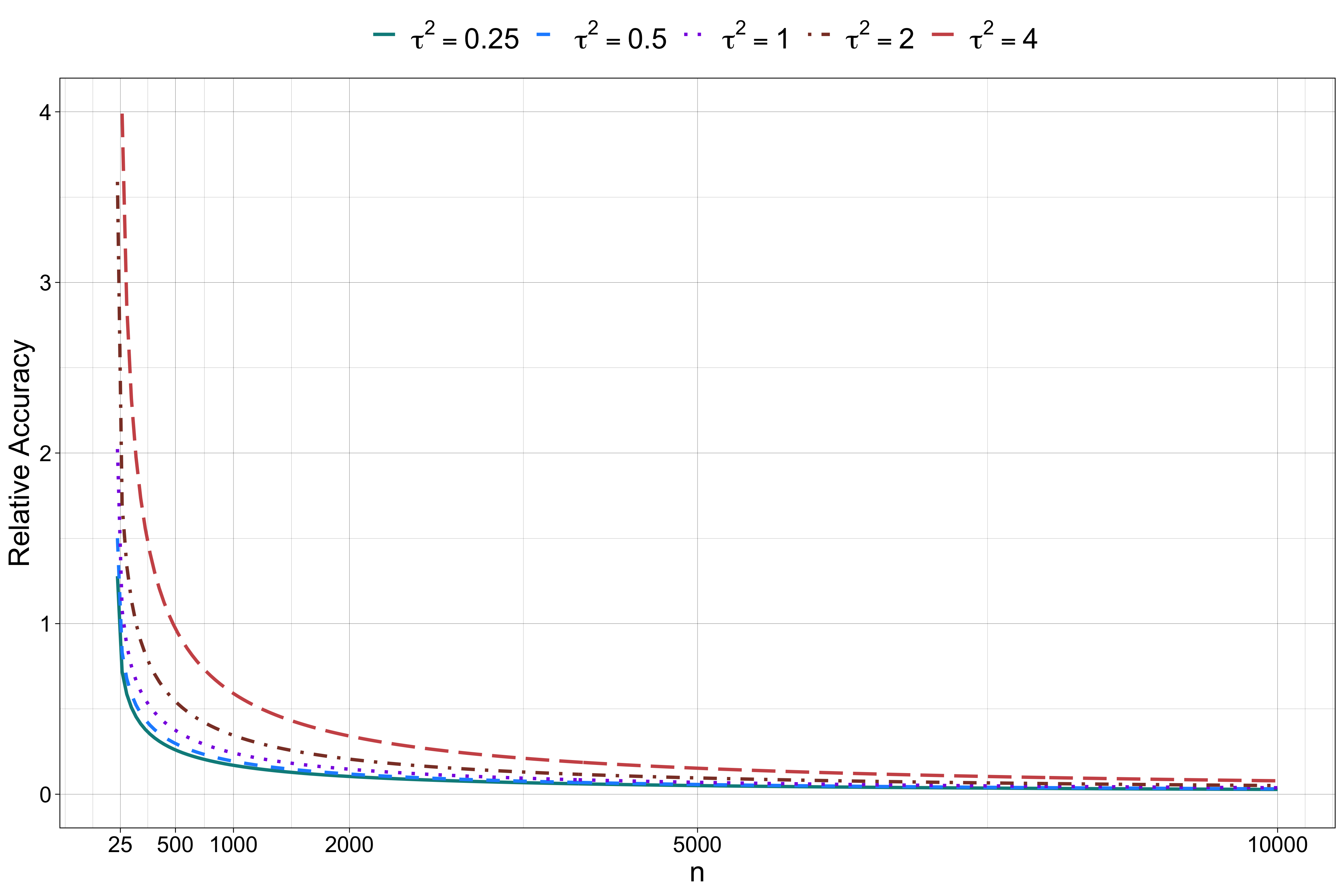
We revisit our simple running example in Section 3 to instantiate Algorithm 1. In the selection stage, we solve (3) with $\omega\sim\mathcal{N}_{2}(0,\tau^{2}I_{2})$ where $\tau^{2}$ is the randomization variance. Before noting the updates from the surrogate posterior, we assess in Figure 3 the relative accuracy of the (generalized) Laplace approximation in (15) with respect to the exact normalizing constant. Because we have exactly one selected group of covariates, the exact normalizer is a one-dimensional integral that can be computed numerically. Especially, we observe how the relative accuracy of the approximation varies with sample size $n$ and randomization variance $\tau^{2}$. For any fixed sample size, the accuracy of approximation for the integral with the mode decreases as the randomization variance increases or, equivalently the concentration of probability mass in the integrand has a greater spread. As expected, we observe that the relative accuracy converges to $0$ with growing sample size for all values of randomization variance.

Now, we exemplify Algorithm 1 for the simple example. Applying Theorems 4.1 and 4.2, (Laplace) in this instance solves the one-dimensional optimization

where $\bar{P}=U^{\intercal}(2\cdot I_{2}-UU^{\intercal})^{-1}$, $\bar{q}=-1$, $\bar{\Sigma}=1+U^{\intercal}(2\cdot I_{2}-UU^{\intercal})^{-1}U$ and $U$ is the unit vector in $\mathbb{R}^{2}$ from writing the Group LASSO solution in the polar coordinate system. The Jacobian function is given by $J^{\star(k)}=(1+\gamma^{\star(k)})^{-1}$. We generate our prototype update for $\beta_{E}^{(k+1)}$ that depends on the expression for the gradient of the surrogate in Theorem 4.2.

At last, we briefly comment on the case when $\sigma$, the error variance in the data, is treated as an unknown parameter. Using a joint prior on $(\beta_{E},\sigma)$ in conjunction with our selection-informed likelihood gives us Bayesian inference in this situation. As prescribed in Panigrahi et al. 2021, one could run a Gibbs sampler that alternates between drawing (i) an update for $\beta_{E}$ given $\sigma$ and (ii) an update for $\sigma$ given $\beta_{E}$. Note, the updates for $\beta_{E}$ based on a gradient-based sampler will assume the expression in Theorem 4.2, except now the gradient of the prior is with respect to the parameter vector $\beta_{E}$.

One approach for the overlapping Group LASSO recovers superposed groups by augmenting the covariate space with duplicated predictors (Jacob et al. 2009). We proceed by implementing the solver (3) with a randomization variable $\omega^{*}\sim\mathcal{N}_{p^{*}}(0,\Omega)$ such that $p^{*}$ is the number of covariates after duplication. To formalize the setting, we let $X^{*}\in\mathbb{R}^{n\times p^{*}}$ denote the augmented matrix of covariates constructed from $X\in\mathbb{R}^{n\times p}$, given that these overlapping groups are determined before selection. Each set of selected covariates $E^{*}$ in the augmented space maps to a set of selected variables $E$ in the original space by reversing the duplication. The stationary mapping for the overlapping Group LASSO with augmented matrix $X^{*}$ and randomization $\omega^{*}$, which we call $\phi^{*}$, is given by

where $\hat{\beta}_{E}$ and $N_{E}=(X^{*})^{\intercal}(y-X_{E}\hat{\beta}_{E})$ are the refitted and the ancillary statistics in our selected model (cf. (5)). Following our notation,

represent a polar decomposition of the overlapping Group LASSO solution; let $U^{*}=\operatorname{diag}\left(\left(u^{*}_{g}\right)_{g\in\mathcal{G}_{E^{*}}}\right)$. Finally,

are the subgradient variables from the Group LASSO penalty for the non-selected groups in the augmented predictor space.

The conditioning event we study for an analytically feasible selection-informed posterior is given by

where $E^{*}$, $\mathcal{U}^{*}$ and $\mathcal{Z}^{*}$ are the corresponding observed instances. We then recover an expression for the adjustment factor along the lines of Theorem 4.1 using the matrices

from the mapping in (17).

References

- Auslender [1999] Alfred Auslender. Penalty and barrier methods: a unified framework. SIAM Journal on Optimization, 10(1):211–230, 1999.
- Barch et al. [2013] Deanna M. Barch, Gregory C. Burgess, Michael P. Harms, Steven E. Petersen, Bradley L. Schlaggar, Maurizio Corbetta, Matthew F. Glasser, Sandra Curtiss, Sachin Dixit, Cindy Feldt, Dan Nolan, Edward Bryant, Tucker Hartley, Owen Footer, James M. Bjork, Russ Poldrack, Steve Smith, Heidi Johansen-Berg, Abraham Z. Snyder, and David C. Van Essen. Function in the human connectome: Task-fMRI and individual differences in behavior. NeuroImage, 80:169–189, October 2013. ISSN 1053-8119. doi: 10.1016/j.neuroimage.2013.05.033.
- Benjamini [2020] Yoav Benjamini. Selective inference: The silent killer of replicability. Harvard Data Science Review, 2(4), 2020.
- Berk et al. [2013] Richard Berk, Lawrence Brown, Andreas Buja, Kai Zhang, Linda Zhao, et al. Valid post-selection inference. The Annals of Statistics, 41(2):802–837, 2013.
- Brett et al. [2002] Matthew Brett, Jean-Luc Anton, Romain Valabregue, and Jean-Baptiste Poline. Region of interest analysis using an SPM toolbox. In Presented at the 8th International Conference on Functional Mapping of the Human Brain, June 2002. Abstract Available in NeuroImage, Vol 16, No 2.
- De Acosta [1992] A De Acosta. Moderate deviations and associated laplace approximations for sums of independent random vectors. Transactions of the American Mathematical Society, 329(1):357–375, 1992.
- Fithian et al. [2014] William Fithian, Dennis Sun, and Jonathan Taylor. Optimal inference after model selection. arXiv preprint arXiv:1410.2597, 2014.
- Gao et al. [2020] Lucy L Gao, Jacob Bien, and Daniela Witten. Selective inference for hierarchical clustering. arXiv preprint arXiv:2012.02936, 2020.
- Glasser et al. [2013] Matthew F. Glasser, Stamatios N. Sotiropoulos, J. Anthony Wilson, Timothy S. Coalson, Bruce Fischl, Jesper L. Andersson, Junqian Xu, Saad Jbabdi, Matthew Webster, Jonathan R. Polimeni, David C. Van Essen, and Mark Jenkinson. The minimal preprocessing pipelines for the Human Connectome Project. NeuroImage, 80:105–124, October 2013. ISSN 1053-8119. doi: 10.1016/j.neuroimage.2013.04.127.
- Inglot and Majerski [2014] Tadeusz Inglot and Piotr Majerski. Simple upper and lower bounds for the multivariate laplace approximation. Journal of Approximation Theory, 186:1–11, 2014.
- Jacob et al. [2009] Laurent Jacob, Guillaume Obozinski, and Jean-Philippe Vert. Group Lasso with Overlap and Graph Lasso. In Proceedings of the 26th Annual International Conference on Machine Learning, ICML ’09, pages 433–440, New York, NY, USA, 2009. ACM. ISBN 978-1-60558-516-1. doi: 10.1145/1553374.1553431.
- Lee et al. [2016] Jason D. Lee, Dennis L. Sun, Yuekai Sun, and Jonathan E. Taylor. Exact post-selection inference with the LASSO. The Annals of Statistics, 44(3):907–927, November 2016.
- Liu et al. [2018] Keli Liu, Jelena Markovic, and Robert Tibshirani. More powerful post-selection inference, with application to the LASSO. arXiv preprint arXiv:1801.09037, 2018.
- Loftus and Taylor [2015] Joshua R Loftus and Jonathan E Taylor. Selective inference in regression models with groups of variables. arXiv preprint arXiv:1511.01478, 2015.
- Marcus et al. [2011] Daniel Marcus, John Harwell, Timothy Olsen, Michael Hodge, Matthew Glasser, Fred Prior, Mark Jenkinson, Timothy Laumann, Sandra Curtiss, and David Van Essen. Informatics and data mining tools and strategies for the Human Connectome Project. Frontiers in Neuroinformatics, 5, 2011. ISSN 1662-5196. doi: 10.3389/fninf.2011.00004.
- Panigrahi [2018] Snigdha Panigrahi. Carving model-free inference. arXiv preprint arXiv:1811.03142, 2018.
- Panigrahi and Taylor [2018] Snigdha Panigrahi and Jonathan Taylor. Scalable methods for Bayesian selective inference. Electronic Journal of Statistics, 12(2):2355–2400, 2018.
- Panigrahi and Taylor [2022] Snigdha Panigrahi and Jonathan Taylor. Approximate selective inference via maximum likelihood. Journal of the American Statistical Association, Forthcoming, 2022.
- Panigrahi et al. [2020] Snigdha Panigrahi, Shariq Mohammed, Arvind Rao, and Veerabhadran Baladandayuthapani. Integrative Bayesian models using post-selective inference: a case study in radiogenomics. arXiv preprint arXiv:2004.12012, 2020.
- Panigrahi et al. [2021] Snigdha Panigrahi, Jonathan Taylor, and Asaf Weinstein. Integrative methods for post-selection inference under convex constraints. Annals of Statistics, 49(5):2803–2824, 2021.
- Petersen and Pedersen [2008] KB Petersen and MS Pedersen. The Matrix Cookbook. Technical University of Denmark, 15, 2008.
- Power et al. [2011] Jonathan D. Power, Alexander L. Cohen, Steven M. Nelson, Gagan S. Wig, Kelly Anne Barnes, Jessica A. Church, Alecia C. Vogel, Timothy O. Laumann, Fran M. Miezin, Bradley L. Schlaggar, and Steven E. Petersen. Functional network organization of the human brain. Neuron, 72(4):665–678, November 2011. ISSN 0896-6273. doi: 10.1016/j.neuron.2011.09.006.
- Rockafellar [2015] Ralph Tyrell Rockafellar. Convex analysis. Princeton university press, 2015.
- Schultheiss et al. [2021] Christoph Schultheiss, Claude Renaux, and Peter Bühlmann. Multicarving for high-dimensional post-selection inference. Electronic Journal of Statistics, 15(1):1695–1742, 2021.
- Shang et al. [2015] Xiaocheng Shang, Zhanxing Zhu, Benedict Leimkuhler, and Amos J Storkey. Covariance-controlled adaptive langevin thermostat for large-scale bayesian sampling. Advances in Neural Information Processing Systems, 28:37–45, 2015.
- Simon and Tibshirani [2012] Noah Simon and Robert Tibshirani. Standardization and the group lasso penalty. Statistica Sinica, 22(3):983, 2012.
- Simon et al. [2013] Noah Simon, Jerome Friedman, Trevor Hastie, and Robert Tibshirani. A sparse-group LASSO. Journal of Computational and Graphical Statistics, 22(2):231–245, 2013.
- Sripada et al. [2019] Chandra Sripada, Mike Angstadt, Saige Rutherford, Daniel Kessler, Yura Kim, Mike Yee, and Elizaveta Levina. Basic units of inter-individual variation in resting state connectomes. Scientific Reports, 9(1):1900, February 2019. ISSN 2045-2322. doi: 10.1038/s41598-018-38406-5.
- Sripada et al. [2020] Chandra Sripada, Mike Angstadt, Saige Rutherford, Aman Taxali, and Kerby Shedden. Toward a “treadmill test” for cognition: Improved prediction of general cognitive ability from the task activated brain. Human Brain Mapping, 41(12):3186–3197, 2020. ISSN 1097-0193. doi: 10.1002/hbm.25007.
- Suzumura et al. [2017] Shinya Suzumura, Kazuya Nakagawa, Yuta Umezu, Koji Tsuda, and Ichiro Takeuchi. Selective inference for sparse high-order interaction models. In International Conference on Machine Learning, pages 3338–3347. PMLR, 2017.
- Tanizaki et al. [2020] Kosuke Tanizaki, Noriaki Hashimoto, Yu Inatsu, Hidekata Hontani, and Ichiro Takeuchi. Computing valid p-values for image segmentation by selective inference. In Proceedings of the IEEE/CVF Conference on Computer Vision and Pattern Recognition, pages 9553–9562, 2020.
- Tian and Taylor [2018] Xiaoying Tian and Jonathan Taylor. Selective inference with a randomized response. The Annals of Statistics, 46(2):679–710, 2018.
- Tian et al. [2016] Xiaoying Tian, Snigdha Panigrahi, Jelena Markovic, Nan Bi, and Jonathan Taylor. Selective sampling after solving a convex problem. arXiv preprint arXiv:1609.05609, 2016.
- Van Essen et al. [2013] David C. Van Essen, Stephen M. Smith, Deanna M. Barch, Timothy E. J. Behrens, Essa Yacoub, Kamil Ugurbil, and the WU-Minn HCP Consortium. The WU-Minn Human Connectome Project: An overview. NeuroImage, 80:62–79, October 2013. ISSN 1053-8119. doi: 10.1016/j.neuroimage.2013.05.041.
- Wong [2001] Roderick Wong. Asymptotic approximations of integrals. SIAM, 2001.
- Yang et al. [2016] Fan Yang, Rina Foygel Barber, Prateek Jain, and John Lafferty. Selective inference for group-sparse linear models. In Advances in Neural Information Processing Systems, pages 2469–2477, 2016.
- Yekutieli [2012] Daniel Yekutieli. Adjusted Bayesian inference for selected parameters. Journal of the Royal Statistical Society: Series B (Statistical Methodology), 74(3):515–541, 2012.
- Yuan and Lin [2005] Ming Yuan and Yi Lin. Model selection and estimation in regression with grouped variables. Journal of the Royal Statistical Society: Series B, 68(1):49–67, 2005.
- Zhao and Panigrahi [2019] Qingyuan Zhao and Snigdha Panigrahi. Selective inference for effect modification: An empirical investigation. Observational Studies, 5(2):131–140, 2019.
Appendix A Proofs for technical developments (Section 4)
Proof of Theorem 4.1.
We write our adjustment factor as follows:
Next, the change of variables in (13) together with the conditioning upon and results in the below simplification