Rigorous treatment of the orbifold model with brane-Higgs couplings
Abstract
We build rigorously the attractive five-dimensional model where bulk fermions propagate along the orbifold and interact with a Higgs boson localised at a fixed point of the extra dimension. The analytical calculation of the fermion mass spectrum and effective Yukawa couplings is shown to require the introduction of either Essential Boundary Conditions (EBC) imposed by the model definition or certain Bilinear Brane Terms (BBT) in the action, instead of the usual brane-Higgs regularisations. The obtained fermion profiles along the extra dimension turn out to undergo some discontinuities, in particular at the Higgs brane, which can be mathematically consistent if the action is well written with improper integrals. We also show that the parity transformations in the bulk do not affect the fermion chiralities, masses and couplings, in contrast with the EBC and the BBT, but when extended to the fixed points, they can generate the chiral nature of the theory and even select the Standard Model chirality set-up while fixing as well the fermion masses and couplings. Thanks to the strict analysis developed, the duality with the interval model is scrutinised.
1 Introduction
As it is well known since the 2000s, the paradigm of models with additional spatial dimensions 11 1 Together with the composite Higgs models which are dual models via the AdS/CFT correspondance. constitutes an attractive alternative to supersymmetry for addressing the Standard Model (SM) puzzle of the gauge hierarchy. Furthermore, the warped dimension framework Randall:1999ee with SM fermions in the whole bulk Chang:1999nh offers an elegant geometrical principle of fermion profile overlap generating the SM fermion mass hierarchy Gherghetta:2000qt (see concrete application models e.g. in Ref. Huber:2001ug; Casagrande:2008hr; Chang:2005ya; Moreau:2005kz; Moreau:2006np; Bouchart:2008vp). In order to realise these two hierarchical features, the Brout-Englert-Higgs scalar field Englert:1964et; Higgs:1964ia, which is at the origin of the SM particle masses through the electroweak symmetry breaking, must be stuck at the so-called TeV-brane 22 2 Let us mention here other possible phenomenological motivations, as from neutrino mass models, for the Higgs boson to be stuck at the boundary of an interval Dienes:1998sb; Abada:2006yd; Grossman:1999ra; Huber:2002gp; Moreau:2004qe or for fermions to propagate in the bulk Frere:2003hn; Nortier:2020lbs. (or located in the bulk with a wave function strongly peaked at this brane). The TeV-brane is a 3-brane (three spatial dimensions) possibly at a boundary of the finite warped extra dimension 33 3 See for instance Ref. Ledroit:2007ik; Bouchart:2009vq; Djouadi:2006rk; Djouadi:2007eg; Djouadi:2007fm; Djouadi:2009nb; Djouadi:2011aj; Angelescu:2017jyj for its phenomenology and Ref. Bouchart:2011va in a supersymmetric context.. More generally, a brane is an hypersurface located in an higher-dimensional space. It can arise in the context of string theories as D-branes which are dynamical objects with quantum properties Polchinski:1996na; Bachas:1998rg (see also Ref. Aharony:1999ti; Duff:1996zn for the supergravity limit of string theories) 44 4 See Ref. Fichet:2019owx; Nortier:2020vge for brane-world effective field theories..
In this paper, we will study the original version Randall:1999ee of the warped dimension scenario based on the orbifold Dixon:1985jw; Dixon:1986jc where the extra space is compactified on a circle respecting a spatial parity of the Lagrangian 55 5 An orbifold being defined as an extra compact manifold with so-called fixed points where the introduced spatial transformation (element from a discrete group ) – letting the Lagrangian invariant – is just equivalent to the identity. It is noted and possesses thus singularities, not like a smooth manifold Quiros:2003gg; Choi:2020dws.. Focusing our attention on the subtle bulk fermion interactions with the brane-Higgs field localised at a fixed point, we will analyse the toy model with a flat extra dimension and the minimal field content: the results obtained on the fermion-Higgs coupling structure are directly applicable to the realistic warped model.
We will clarify the treatment of the bulk fermion couplings to the brane-localised Higgs boson, within the orbifold background, by building rigorously the four-dimensional (4D) 66 6 Including time. effective Lagrangian of the minimal model, that is by calculating consistently the Kaluza-Klein (KK) tower spectrum of fermion mass eigenvalues and the 4D effective Yukawa couplings (via the fermion wave functions along the extra dimension).
In particular, we will demonstrate that no brane-Higgs regularisation [like smoothing the Higgs Dirac peak] should be applied (not necessary and no theoretical argument for it) in contrast with the usual regularisation procedure of literature (see Ref. Angelescu:2019viv and references therein) and that, instead, one must introduce either Essential Boundary Conditions (EBC) on 5D fields 77 7 Directly imposed by the model definition, in contrast with the Natural Boundary Conditions (NBC) deduced from the action minimisation condition., originating from the symmetry, or equivalently some Bilinear Brane Terms (BBT) in the fundamental 5D Lagrangian. The exact matching of the fermion mass spectra derived respectively through 4D and 5D methods will be used in order to confirm our analytical results. All those statements (except the 4D approach) hold as well for the free case i.e. without Yukawa interactions.
This necessity of the presence of EBC or BBT (terms with the same form as in Ref. Angelescu:2019viv; Nortier:2020xms), in the 4D or 5D approach, has been found as well Angelescu:2019viv in the finite interval scenario (the higher-dimensional framework of the other warped model version) with identical brane-Higgs couplings to bulk fermions: this conclusion confirms that a specific treatment is required for point-like interactions between bulk fermions and brane-Higgs bosons in higher-dimensional spaces.
Besides, we will strictly describe and work out the entire known duality: identical physical quantities, namely the mass eigenvalues and 4D effective Yukawa couplings, are obtained in the different orbifold scenario with the Higgs boson localised at a fixed point and finite interval geometrical set-up with the Higgs field stuck at a boundary.
The EBC and BBT (forms including signs) choices, which should originate from an Ultra-Violet (UV) completion of the theory, turn out to induce the chiral nature of the low-energy effective theory as well as realising the specific SM fermion chiralities. Indeed, all these chirality properties are in fact not selected by the remaining sign choices for the 5D fields transformed via the spatial group – as the solutions we find within this orbifold configuration can exhibit twist transformations (sign modification here) of the 5D fields, à la Scherk-Schwarz Scherk:1979zr; Cremmer:1979uq, through the extra space reflection. We will even show that the transformation sign choices are just mathematical conventions without physical impacts on the SM field chiralities, the fermion mass spectrum and the 4D effective Yukawa couplings.
Nevertheless, in order to clarify the chirality aspects, we will also study a different scenario – considered for example in Ref. Gherghetta:2000kr – where the transformation definitions on the fields cover as well the fixed points themselves. It turns out that the associated transformation sign choices precisely at these fixed points constitute here additional EBC, noted EBC’, that have the capacity to select some of the previous EBC and hence to fix the chirality set-up. Once more, the rôle of these EBC’ can be played instead by certain of the above BBT. Interestingly, such an inclusive symmetry definition can induce by itself the chiral nature of the theory as well as the SM chirality distribution over the various fields. This origin for the whole chirality configuration is not offered within the simpler interval model for instance. In the presence of brane-localised Yukawa couplings, such an inclusive scenario can only be treated through the 4D method. The fermion masses and couplings are also affected by this inclusive symmetry.
The action integral definition and integral domain end-points will be treated carefully. In particular the decomposition of the action to introduce improper integrals will appear to be required in the presence of orbifold fixed points or point-like fermion-boson interactions (not located at the boundary of a finite extra space like an interval). Within this new and appropriate approach of the specific points along the extra dimension of the orbifold, we find for the free or Yukawa case that some of the obtained consistent solutions exhibit certain field jumps at these fixed points and localised-interaction point. This interesting result of the possible existence of consistent profile jumps stands against one’s first intuition Csaki:2003sh; Azatov:2009na, but those jumps are only induced by sign flipping and not by point-like changes of the absolute value of the wave function amplitudes.
The analysis of the present orbifold background with brane-localised fermion-scalar interactions, as well as the previous results Angelescu:2019viv on the interval background, show that generally speaking the action expression does not systematically contain all the information allowing to fully define the model: in particular some EBC may be used (in contrast, the BBT are terms in the action) depending on the brane treatment adopted or on the UV completion of the theory (which could introduce the BBT).
2 Minimal consistent model
2.1 Geometry and symmetries: the proper action
We consider the 5D space-time model with the product geometry described just below.
- •
represents the usual 4D Minkowski space-time whose coordinates are denoted by where is the Lorentz index of the covariant formalism. The metric conventions are given in Appendix A.
- •
stands for the extra space orbifold obtained from modding out the circle by the discrete group 88 8 Factor element, , and neutral element, . symmetry .
This circle is characterised by a radius and its coordinate is , not double-counting the point since it is this point, by pure convention, that is chosen to be the junction point geometrically identified with the point (which we note: ) 99 9 Another possible mathematical convention would have been, for instance, . in order to implement the circle periodicity. The circle could be constructed from the real axis by imposing a periodicity, that is by identifying geometrically an infinite number of translated regions of size and hence by limiting the 1D space to the fundamental domain .
The (non-neutral) transformation on space, 1010 10 The convention above, of having taken the coordinate origin at the strict middle of the circle domain (or fundamental domain), renders the parity with respect to the origin more explicit and convenient to study., has a representation on a generic 5D field,(1) which must let the Lagrangian density invariant, by definition of the symmetry:
(2) We mention that this equation can define a class of equivalence of a given coordinate , defined as with , as illustrated symbolically on Fig. 1.
Two fixed points arise: and . At these fixed points, the Lagrangian condition of Eq. (2) is automatically satisfied: , and, , so that is naturally taken as the identity operator in Eq. (1) since no transformation needs to apply on the fields there. Another scenario will be analysed in Section 6.

In order to properly write down the initial action, we urge the importance of taking care of possible field jumps along the extra dimension upon the reader. We are going to show that the existence of a field jump in field theory can make sense mathematically if the action integration domain is properly divided at the jump location. Different discontinuity configurations must be considered. First, the hypothesis of a possible jump at any point of the bulk would lead to an infinite number of cuts in the action integration region which would obviously not be treatable leading to unpredictable observables: this assumption is thus excluded. Secondly, assuming an arbitrary finite number of possible jumps and hence of mathematical separations in the action domain, outside the fixed points, is not expected to affect the unique physical results – like the fermion mass spectrum – since none of those jump points exhibit some specific property: it is thus useless to explore this direction. Thirdly, the case of possible profile jumps at the two specific points that are the fixed points of the orbifold – one of those two, , corresponding as well to the Yukawa coupling location (see Section 2.2.3) – remains to be studied. The effective presence of such profile jumps in some of the obtained solutions (see Figures 2 and 3 respectively for the free and coupled fermion situations) confirms this possibility. For example, in case of a profile jump at (an identical discussion holds for the other fixed point at ), regarding a well-defined Lagrangian integrand involving 5D fields over the whole action integration domain, we simply have to choose between the mathematical definitions of the left or right continuity for a generic profile function along the extra dimension: with , or, . This choice is conventional and hence cannot affect numerical results, so let us choose conveniently
| (3) |
throughout this paper, in case of jumps at the fixed points. Then, the well-defined global action of this model must be written as a sum of some brane terms, an improper integral and a standard integration over different regions covering the whole physical domain of the circle:
| (4) |
where , represents action terms located at the orbifold fixed points and stands for the fermion kinetic terms of the Lagrangian density (see next subsection). Indeed, all the obtained fields will be well-defined at the two fixed points via Eq. (3). Besides, for to be integrable over the entire region , this Lagrangian density, which will involve profile derivatives , must be well-defined over this region. The necessary (but not sufficient) condition for this last feature is that the profiles have to be continuous on and Eq. (3) also guarantees this continuity. For the consistency of the other integration term in Eq. (4), the profile continuity along 1111 11 To be clear, the integration domain corresponds to the spatial region along the extra dimension – respectively the Francophone and Anglophone notations – which does not include the fixed points at and . obviously reads as:
with , , and similar equalities hold at the other region boundary . Furthermore, the worked out solutions will (well) be derivable over the two regions and (see Sections 3.2 and 5.3 respectively for the free and coupled fermion situations) so that will be well-defined. For example, is derivable in the region at if and only if is right-derivable at , and the corresponding right-derivative does not diverge thanks to the first equality of Eq. (3). Notice that from the point of view of the integration by pieces of the action in Eq. (4) precisely over the physical domain, the inclusion (or not) of the single points at or does not affect the integral results – given the continuous form of the even over the two regions – so that only consistent action definition arguments were considered here.
2.2 Field content and complete action
2.2.1 Bulk fermion fields
Let us introduce the minimal spin-1/2 field content which allows to write down a SM Yukawa-like coupling between zero mode fermions (of different chiralities) and a spin-0 field (see Section 2.2.3). It is constituted by a pair of fermion fields called and . Those particles propagate along the circle , as we have in mind an extension of this toy model to a realistic scenario with bulk matter (c.f. Section 2.2.4) where will represent respectively the gauge doublet down-component quark and the singlet down-quark.
The 5D fields and – of mass dimension 2 – have the following kinetic terms [entering Eq. (4)] which allow to recover canonical covariant kinetic terms for the associated fermions in the 4D effective action (as imposed by the argument of decoupling limit 1212 12 From the theoretical consistency and phenomenological points of view, the SM must be approximately recovered at low-energies in the limit of infinitely heavy KK excitations.):
| (5) |
using the standard notations , , with for the coordinates and for the 5D Dirac matrices (c.f. Appendix A). In the used conventions, the 5D Dirac spinor, being in the irreducible representation of the Lorentz group, reads for example for as,
| (6) |
in terms of the two two-component Weyl spinors , , standing for the Left/Right chirality, and as usually .
As stated at the end of previous section, the Lagrangian must obey the condition (2). For this purpose, the transformation (1) on the 5D fields and can take four different forms which constitute Essential Conditions (EC) issued from the model definition:
| (7) |
| (8) |
| (9) |
| (10) |
under which the Lagrangian (5) is indeed invariant, as appears by using the properties of the Dirac matrix and the odd parity of the fifth partial derivative . Notice that the parity (second order cyclic group) does not allow complex phase factors in the transformations:
Using the definition of Appendix A together with Eq. (6), we already deduce some information on the possible 5D chiral field parities with respect to , as indicated in Eq. (7)-(10).
Based on Eq. (6), we can rewrite the bulk Lagrangian of Eq. (5) in forms which are convenient to see at a glance the Lagrangian even parity, simply by using the occurence of fixed 5D field parities, different for the Left/Right chiralities [c.f. Eq. (7)-(10)], and the odd parity:
where the low double arrows indicate a replacement of 5D fields in the previous terms and the matrices are defined in Appendix A.
2.2.2 Brane-localised scalar field
The questions about the mass calculation arise when the bulk fermions couple to a single 4D real scalar field (mass dimension 1) which is confined at a fixed point of the orbifold, as in the studied model (inspired by the warped scenario addressing the gauge hierarchy problem). We simply choose this fixed point to be at , rather than , which is a purely mathematical convention since these two points belong to a circle. The real scalar field has an action of the generic form,
| (11) |
with a potential possessing a minimum which generates a non-vanishing Vacuum Expectation Value (VEV) for the field expanded as
| (12) |
in analogy with the SM Higgs field.
2.2.3 Yukawa interactions
We consider the following Yukawa interactions allowing to study the subtleties induced by the coupling of the above brane-scalar field (at ) to the introduced bulk fermions,
| (13) |
Notice that considering operators involving the fields , , up to dimension 5 allows to include such a Yukawa coupling. Let us recall here that in case of profile jumps at the fixed point at , the 5D fields , are defined through the profile convention (3), as already described. The studied model with a Yukawa coupling at a fixed point will turn out to be dual to the interval model including a Yukawa coupling at a boundary (see Section 7).
The complex and Yukawa coupling constants, entering Eq. (13), are independent and a well-defined 4D chirality holds for the fermion fields on the 3-brane strictly at Angelescu:2019viv; Azatov:2009na. To avoid the introduction of a new energy scale, in the spirit of the warped model, we can define the 5D Yukawa coupling constants as
| (14) |
where , are dimensionless coupling constants of . Then, can be approximately identified with the SM Yukawa coupling constant within the decoupling limit, as will be described in Eq. (91)-(92).
When calculating the tower of excited fermion masses, we restrict our considerations to the VEV of and concentrate our attention on the following part of the action (13),
| (15) |
with the compact notations and . Based on Eq. (12), the complete action reads as, , with the localised fermion-scalar interaction terms:
| (16) |
that allow to work out the 4D effective Yukawa coupling constants.
2.2.4 Bilinear brane terms
Introducing all the covariant operators up to mass dimension 5 [like for the Yukawa couplings (13)] in this model, one should consider as well the dimension 4 operators given just below, that we call the BBT like in Ref. Angelescu:2019viv. Furthermore, the presence of the BBT has several justifications: (i) they allow to avoid physical consistency problems both in the free case (see Sections 3.1 and 3.3) and with Yukawa couplings (Sections 5.1 and 5.3); (ii) they play the rôle of defining well the model at the two orbifold fixed points both in the free case (see Sections 3.2 and 3.3) and with Yukawa couplings (Section 5.3); (iii) they induce the expected matching of the analytical results on the spectrum derived through the 4D and 5D approaches (see Sections 4 and 5.3).
The following BBT lead to the SM chirality configuration,
| (17) |
where , and for example . Indeed, without Yukawa couplings, these terms will induce only a non-vanishing profile [see line 2 of Eq. () and Table 1 in case of the zero-mode with mass ] in the 5D field so that only the Left-handed 4D field will exist. This zero-mode , without KK mass contribution, constitutes the lightest mode of the KK tower and also the SM state. Hence, we can well recover the SM configuration: a chiral field content and a Left-handed 4D field potentially representing the quark doublet in the direct extension to gauge symmetries (and three flavours). Given that, similarly, the BBT (17) will exclusively lead to a Right-handed 4D field [line 1 of Eq. ()] potentially representing the SM down quark type (gauge singlet). When adding the Yukawa couplings (13), this SM chirality set-up remains though it is no more explicit due to the - mixing, via vector-like KK state mixings, which induces some vector-like mass eigenstates for the lightest modes of the tower (see Sections 4 and 5.3). In the decoupling limit where heavy KK state mixings tend to vanish, the SM chirality configuration is recovered as expected.
For completeness, let us underline that in the free case, the opposite BBT signs, , , would lead to a chiral set-up for the zero-modes but different from the potential SM chirality configuration, namely: . Similarly, the BBT signs, , , would lead to the set-up, , and, , , to, .
Finally, as will be described in the Sections 3.2 and 3.3, the possible signs, (same sign for and ), would instead lead to the profile solutions () with two non-vanishing profiles for the lightest modes (as ) and hence to vector-like states: . The same statement holds for and thus . Such massive vector-like states 1313 13 Extensive phenomenology at colliders has been developed about such vector-like particles Azatov:2012rj; Bonne:2012im; Moreau:2012da; Gopalakrishna:2013hua; Angelescu:2015kga. can be used to build custodially protected warped models Agashe:2003zs and are then called custodians (see for instance Ref. Bouchart:2008vp). Of course there exist 8 remaining cases combining the above Lagrangian sign configurations: , , and, , .
Therefore, it appears clearly that the BBT control the chiral configurations of the model. The UV completion of the theory can be at the origin of the BBT and hence of the chirality set-up: chiral nature of the theory and specific chiralities of the various fields.
To end up this section, we note that the complete toy model studied is characterised by the action,
| (18) |
The conclusions that will be derived in the present work can be directly extended to the realistic warped model with SM bulk matter addressing the fermion mass and gauge hierarchies, along the same lines as the flavour and gauge symmetry generalisations described in details in the Section 2.6 of Ref. Angelescu:2019viv.
3 Free bulk fermions on the orbifold
In this section, we calculate the fermionic mass spectrum for the free case where in the action piece given by Eq. (13).
3.1 Applying the NBC
We start by considering the bulk action part,
of Eq. (4), from the considered action, , of Eq. (18). We apply the least action principle to it which leads to two relations of the kind, , one for each of the unknown 5D fields , and two corresponding ones, , involving the complex conjugate fields 1414 14 The equations of motion and boundary conditions derived from the least action principle for the fields and their conjugates are trivially related through the Hermitian conjugation., since the elementary field variations , , and (see Appendix B.1) are generic and hence independent from each other. Using compact notations, like for example,
we can write in particular 1515 15 We omit the global 4-divergence which vanishes in the action integration due to vanishing fields at the boundaries at infinities. Indeed, when minimising the action, the varied terms must vanish separately at infinite boundaries, since the non-vanishing field variations at boundaries are independent from each other and from the bulk ones (see also Ref. Peskin:1995ev). This is realised by the local physics statement which induces vanishing fields at infinities due to the wave function normalisation conditions (see also Ref. Schwartz:2013pla).,
| (19) |
Based on the Lagrangian of Eq. (5), these two bulk terms take the same form (the first one being calculated explicitly in Eq. (113) to clarify the spinor component treatment) and the two remaining brane terms can be calculated as well:
| (20) |
where we have further invoked the transformations (7)-(10) for the generic 5D field, Eq. (114) for its variation and properties:
Then thanks to Eq. (3) 1616 16 Those continuity relations lead to , i.e. [c.f. Eq. (109)], and in turn to which can be written as via Eq. (110). Similarly we get . and Eq. (111)-(112), respectively, the expression (20) simplifies to,
| (21) |
In this expression, the bulk and brane variations – respectively the volume and surface terms – must vanish separately due to independent field variations (no reason to be linked). Besides all those field variations are not vanishing (unknown fields) so that we get the bulk Equations Of Motion (EOM),
| (22) |
and the Natural Boundary Conditions (NBC),
| (23) |
At this level, we can first solve Eq. (22) together with Eq. (23) to find out the fields over the domain, . This is precisely what has been done in the preliminary Ref. Angelescu:2019viv where the two exactly identical Eq. (3.3) and (3.4) [there] have been solved over the interval, . Since the fields are continuous over [c.f. Eq. (3)] like there over , we can thus apply here the results obtained in this reference: the solutions found for Eq. (22)-(23) are expressed through the KK decomposition (with a similar choice of global factor),
| (24) |
where the 4D fields represent the KK states and satisfy the Dirac-Weyl equations,
| (25) |
involving the KK mass eigenvalues , while the only resulting profiles , , included respectively into , are vanishing over . The opposite signs in front of each mass term of the bulk profile EOM induced by Eq. (22), with respect to the calculations of Ref. Angelescu:2019viv, just originate from a different sign convention for the matrix [see Eq. (107)] and hence do not modify the (un)physical result of vanishing profiles. Now let us study the profile solutions in the complementary region, . Inserting the KK decomposition (24) into the first type of transformation (7), one obtains the transformations directly on the profiles ():
| (26) |
where the implications come from the linear independence of mass eigenstates . Similarly, for the three other types of transformations (8)-(10), we have the following profile parities:
Therefore, all the profiles are systematically vanishing on the whole orbifold region, . Such profiles conflict with the two (for ) ortho-normalisation conditions over the full domain,
| (50) |
originating from the condition of a canonical form for the 4D effective kinetic terms. Hence the solutions for the fields obtained through this first method are not physically consistent.
3.2 Introducing the EBC
In fact, one necessary ingredient was missing in the naive approach of Section 3.1. In order to identify it, we have to study the conserved fermion probability currents corresponding, via the Noether’s theorem, to the global and symmetries of the action,
involving the Lagrangian (5). The two independent global transformations of the fields, letting invariant, act respectively as,
| (51) |
where () are continuous constants entering for instance the infinitesimal field variations 1717 17 Different clear notations are used here for the infinitesimal field variations under specific transformations, , and the above generic field variations in the variation calculus context of the least action principle, [see typically Eq. (110)].:
Choosing instead to consider a unique symmetry ( for any field ) would correspond to a particular case only, among the general Lagrangian symmetry possibilities. Besides, this particular case would not provide the maximal information, since one symmetry would be associated to only one conserved probability current. We thus well consider, in this subsection, the transformations (51) [with both possibilities, or ] and the two independent symmetries. Based on these two symmetries, and the bulk EOM whose standard structure appears in Eq. (19), the Noether’s theorem predicts the local conservation relation,
| (52) |
for the two probability currents,
| (53) |
as derived in details within the Appendix B of Ref. Angelescu:2019viv. This relation holds over the whole orbifold domain, , since the sole bulk terms in the action infinitesimal variation – under transformation – must vanish for any integration sub-region included inside the entire integration domain of the action precisely defined for the model. The mathematical consistency of the condition (52) imposes necessarily continuous 5-current components over all the model space-time and in particular a continuous along 1818 18 Notice that this condition is in agreement with Eq. (3) which guarantees continuous fields along .. Furthermore, a jump of the form, , would not determine any field at the fixed point and thus would not lead to vanishing variations in Eq. (20) that would modify the BC (23) inducing non-physical solutions. A similar argument applies at the other fixed point, . Hence, one has to consider the remaining model possibility, and 1919 19 A change must occur at both fixed points to cure the problems of the solutions worked out in previous subsection. , so that this current component is continuous over all the range, . In particular, we can now write,
| (54) |
This obtained relation must be compared with the following one, coming directly from the transformations of type (7)-(10) and properties,
| (55) |
The combination of Eq. (54) and Eq. (55) gives rise to a vanishing current component at the fixed point:
Similar arguments regarding the second fixed point imply obviously that,
so that, using the generic chiral decomposition (112), we get the following current conditions,
| (56) |
leading to the minimal Boundary Conditions (BC),
| (57) |
These BC induce systematically the vanishing of all the brane terms in the varied action obtained in Eq. (21). Indeed, for example, the fixed value implies and in turn 2020 20 Rigorously speaking, the action should not be minimised with respect to the known fixed fields so that the terms with vanishing field variations should not even appear. In fact, the brane terms of Eq. (21) should originally be written as a generic sum over unfixed fields. [considering more precisely their two respective components as is clear from Appendix B.1]. Therefore the sole remaining BC are those of Eq. (57): there are no more NBC generated from the brane terms of Eq. (21) and we name the BC (57) as EBC since they are imposed by the transformations (55) which contribute to define the studied model. From the point of view of the methodology, notice interestingly that it was necessary to consider the fermion probability currents to reveal the existence of the EBC. Now, solving the new EBC (57) together with the unchanged bulk EOM (22) over the domain, , was precisely realised in Ref. Angelescu:2019viv where the same Eq. (3.3) and (3.16) [there] were solved over the interval, . Once more, since the fields are continuous over [see Eq. (3)] like there over , we can apply here the results derived in this previous work: the 5D solutions found for Eq. (22)-(57) are given by Eq. (24)-(25) and the following four possible sets of profiles over together with the associated KK mass spectrum equations (),
and,
The opposite signs in front of the and profiles, with respect to the results in Ref. Angelescu:2019viv, just come from a different sign convention for the matrix, between here [see Eq. (107)] and this reference. In Eq. ()-(), we use the standard BC notations, i.e. or for instance at stands respectively for the Dirichlet or Neumann BC: or . For example, the symbolic notation denotes Dirichlet (Neumann) BC at (). These notations make explicit the correspondence between the four EBC (57) and the four solutions ()-(). The equation possesses the following solutions for the KK mass spectrum,
| (60) |
Similarly, the equation has the solutions:
| (61) |
The part of the general solutions in the complementary domain, , is now obtained via the four types of transformations (26)-(3.1). Therefore, the inclusion of the EBC based on the vanishing probability currents allows to obtain consistent fermion profile and mass solutions.
| Fields | |||||
| Continuity | |||||
| domains | |||||
| Any | |||||
| I | |||||
| II | |||||
| III | |||||
| IV | |||||
| KK Masses | , | ||||
In Table 1, we present the explicit solutions over the whole orbifold domain for the SM-like profile () taken from line 1 (2) of Eq. (): see the discussion on SM chirality configuration in Section 2.2.4. The mass spectrum for the 4D KK states is defined by Eq. (25) and it is already determined by Eq. (60)-(61). Notice on Table 1 that the same spectrum enters the profile solutions in both regions, , and, . In this table, we also give the general values of the complex constants, in Eq. (), obtained from the ortho-normalisation conditions (50) 2121 21 Here, thanks to the profile parities, a change of variable, , could be applied to recover exclusively the integration domain .. We observe on Table 1 that the choice of type of transformation is just a convention since it can modify the profile signs but it affects neither the mass spectrum nor the fermion chirality configuration – as a certain chiral zero-mode profile vanishing on the region is also systematically vanishing over . In contrast, the chirality configuration and mass spectrum are fixed by the choice of EBC (57) which can lead either to the two kinds of chiral solutions in Eq. () or to the vector-like solutions ().
In Figure 2, we draw the first two excitation profiles for each free solution presented in Table 1 within the simple real case, , and for two different types of transformations from Eq. (26)-(3.1). We see clearly on Figure 2 that for example with the type of transformation, jumps appear for the profiles and at the two fixed points at, , , in the scenario without Yukawa couplings. The presence of profile discontinuities here already justifies the treatment exposed in Section 2.1. The precise prescription (3) regarding the action integration domain, described in this section, renders the jumps of Figure 2 consistent mathematically: the difference, e.g. , is compatible with a well defined Lagrangian integrand over the action integration domain, , where the profiles are continuous.

3.3 Introducing the BBT
As suggested in Section 2.2.4, we can alternatively introduce the dimension 4 operators of Eq. (17) to study their effects with respect to the inconsistencies raised in Section 3.1. Hence, to the action from Eq. (4), we add now another part and consider:
The variations of with respect to the generic field [using Eq. (111)],
together with Eq. (21) allow to write down the variations of the free fermion action:
| (62) |
The individual vanishing of those volume and surface terms lead to the EOM (22) together with the four following NBC, depending on the two choices,
| (63) |
At this level, the EOM and NBC are effectively the same as the EOM (22) and EBC (57) of the previous subsection, in the domain , so that we find again the solutions ()-() together with the mass spectra (60)-(61). For instance, the SM-like choice of Eq. (17) leads via Eq. (63) to the solution of line 2 in Eq. (). Then the parts of the general profile solutions in the complementary region, , are found out via the different types of transformations (26)-(3.1) in the free case, as in Section 3.2, so that the complete solutions are once more identical and can also be illustrated by the Table 1 and Figure 2 both based on the ortho-normalisation conditions (50). In conclusion, introducing the BBT permits to rigorously work out profile and mass solutions. A second conclusion in this approach is that the chirality set-up – one of the two chiral solutions () or of the vector-like ones () – and associated mass spectrum are fixed by the choice of NBC (63) and thus originally by the choices of BBT signs in Eq. (17). In simpler words, the BBT (like the EBC previously) control the chiral nature of the theory as well as each field chirality.
Let us now discuss the probability currents. The addition of the part in Eq. (17) to is not affecting the current equations (52)-(53) since the new brane terms so induced in the infinitesimal action variation – under the transformations (51) – vanish due to their invariant form. In contrast with the previous subsection and with the interval model in the free case with BBT Angelescu:2019viv, there exists no demonstration here of Eq. (56). Nevertheless, we can check that is well vanishing by using the obtained solutions ()-(): the product systematically vanishes at . Therefore, the BBT play the rôle of making vanish ( transformation consequence) like the EBC were guaranteeing it in Section 3.2. Note that we could simultaneously apply the EBC and introduce the BBT but those two processes would be physically redundant to define the model.
4 Brane-localised scalar couplings in the orbifold: 4D approach
Once the free case is addressed, via the EBC (57) in Section 3.2 or the NBC (63) induced by the BBT in Section 3.3, the free fermion mass spectrum and profiles are known. Then how to take into account the effects of the action part in the mass spectrum, the action (15) being induced by the Yukawa interaction between a brane-localised scalar field and bulk fermions? The considered action reads thus as,
| (64) |
A first method called the perturbation method, described in the present section, is performed at the level of the 4D effective Lagrangian, that is by calculating the mass mixings between the different levels of the KK towers. Considering the SM-like profile solutions () and associated free KK mass spectrum from line 1 (2) of Eq. (), all the initial 4D effective masses for the KK modes of Eq. (24) in the interaction basis can be classified into two species: the pure KK masses (60) and the mass contributions from the Yukawa interaction given by the overlap between the wave functions and Higgs-brane,
| (65) |
In particular, as imply the respective SM solutions () so that the coupling constant disappears from the mass dependences. Note that for similar reasons [c.f. Eq. (112)], in case of the presence of the BBT (17), those do not generate 4D mass terms. All the 4D mass terms enter the 4D effective Lagrangian through the following mass matrix,
within the field basis noted,
| (66) |
The texture of this infinite mass matrix involving the diagonal , off-diagonal and mixing the , fields together can be precisely taken from the interval model context Angelescu:2019viv (Section 3.2), with the replacement , since the KK masses and bulk profile solutions are then identical (up to extensions over as seen in Section 3.2 here) like the Yukawa interactions localised at [for any transformation (26)-(3.1)]. Now we can apply the results for the mass eigenvalues of the 4D eigenstates obtained through the bi-diagonalisation performed in this Ref. Angelescu:2019viv, based on the calculations of Ref. Barcelo:2014kha, by re-normalising to since the two present profiles (even or odd) entering are normalised via Eq. (50) over a domain of double size compared to the interval case. Doing so, the obtained exact mass eigenvalues are determined by the following equation, coming from the characteristic equation,
| (67) |
in the case of a real parameter and the positive branch from Eq. (60). Notice that the different conventional sign in front of the profiles found in Eq. () [here and ], with respect to the interval study Angelescu:2019viv, does not affect the final mass spectrum – as is clear from Eq. (65). Hence, the physical absolute value of the mass spectrum reads as:
| (68) |
with the function defined according to,
| (69) |
5 Brane-localised scalar couplings in the orbifold: 5D approach
5.1 Applying the NBC
Let us now study the presence of Yukawa couplings at the fixed point, , through the action,
| (70) |
within the 5D approach, that is by considering the mixings among KK excitation states at the level of the 5D fields. The BBT introduced here at the fixed point at are the ones of Eq. (17) leading to SM-like chirality configurations: , . Those guarantee a correct treatment of the free brane, like the EBC, as analysed throughout Section 3. Using Eq. (62) and Eq. (15), one gets directly the following action variations with respect to the fields and ,
| (71) | ||||
The separate vanishings of these volume and surface terms, induced by the least action principle, give rise respectively to the EOM (22) and the following NBC,
| (72) |
As usual, the 5D field solutions of the EOM (22) and NBC (72) have the form of the following mixed KK decomposition [instead of Eq. (24)] Casagrande:2008hr; Azatov:2009na,
| (73) |
with the 4D fields , already mentioned in Section 4, satisfying the Dirac-Weyl equations,
| (74) |
the being the fermion mass eigenvalues including the contributions from the Yukawa terms and these 4D fields the mass eigenstates including the effects of mixings among the , fields as well as (infinite) KK levels. The explicit profile solutions appearing in Eq. (73) over the domain, , were found out for the interval model studied in Ref. Angelescu:2019viv where the exactly identical EOM and same NBC, up to a sign and a factor in front of each parameter, [respectively Eq. (3.3) and (5.5) there] have been solved over . Because the fields are continuous over [c.f. Eq. (3)] like there over , one can apply here the conclusions obtained in this reference. The opposite sign in front of the parameters originates from a different Dirac matrix sign convention [see the sign in Eq. (107)] and has thus no physical consequences. The relative factors , at the same places in the NBC (72), come from the existence of surface terms both at , and , as is clearly described in Eq. (20)-(21). These factors turn out not to modify the relations between the different profile solutions and to only induce a factor- change in the final mass spectrum equation, both obtained in Ref. Angelescu:2019viv. Besides, the two (for ) following ortho-normalisation conditions over the full domain [replacing Eq. (50)],
| (75) |
as induced by the decomposition (73), can be recast into the integration relations of Ref. Angelescu:2019viv over the region but with a global factor , thanks to the change of variable , the fixed odd/even parities of the profiles and Eq. (3), so that the demonstration about profile solutions on the interval in Ref. Angelescu:2019viv remains unchanged here, from this point of view as well. Indeed, injecting the mixed KK decomposition (73) into the first type of transformation (7), we get the transformations directly on the profiles:
| (76) |
In the same way, for the three other types of transformations (8)-(10), one obtains the same profile parities as in Eq. (3.1). As a conclusion, the same result as in Ref. Angelescu:2019viv holds here for the orbifold: the 4D effective Yukawa coupling constant for the lightest modes (), induced by the found profiles, tends to zero within the decoupling limit which is not compatible with the SM configuration expected. The problematic characteristics of the solutions obtained in this naive approach are confirmed by the final mass spectrum equation, (independent from the profile normalisations), which conflicts analytically with the one obtained through the 4D method in Eq. (67) for a real parameter. This failure motivates the alternative 5D methods of the next two subsections.
5.2 Introducing the EBC
Following the same idea as for the free case in Section 3.2, we try now to find consistent fermion mass solutions via considerations on their currents. The currents permit a priori to fully define the geometrical field configuration like here for the orbifold scenario. The complete relevant action including the brane-localised Yukawa terms (15),
| (77) |
like in Eq. (70), is invariant under the unique symmetry defined via Eq. (51) only for,
| (78) |
since the fermions and are mixed on the brane at . Based on this symmetry involving both and as well as on the bulk EOM [whose standard structure appears in the action variation (19)], the Noether’s theorem predicts (c.f. Appendix B of Ref. Angelescu:2019viv) the new local probability conservation relation,
| (79) |
involving the individual currents given by Eq. (53)-(78) over the full orbifold domain, . Notice that the new brane terms entering the infinitesimal action variation – under the transformations – vanish because of their invariant form and have thus no direct effect on the conservation relation (79). The mathematical consistency of the relation (79) implies necessarily the continuity of 5-current components over the whole space-time and in particular a continuous along . Besides, a discontinuity of the form, , would not fix any field at this fixed point and in turn would not induce vanishing variations in Eq. (71) possibly modifying the BC (72) which induce the drawbacks already pointed out in Section 5.1. As a consequence, we must consider the remaining model possibility:
| (80) |
where Eq. (3) is also invoked. On the other side, the current is odd under any type of transformation (7)-(10) as can be shown in a similar way as in Eq. (55):
| (81) |
Combining Eq. (80) with Eq. (81) leads to,
so that, using Eq. (56) and (78), we get the relation (inducing EBC),
| (82) |
and its variation (for a non-trivial transformation with ),
| (83) | |||
At this level, we can consider the search for field solutions of vanishing Eq. (71) and Eq. (82)-(83) first on the domain, , which is equivalent to the search performed for the interval model in Ref. Angelescu:2019viv with the replacement, . Given that the ortho-normalisation condition (75) written on the domain is the same within the orbifold and interval frameworks, up to an overall factor , we can apply the conclusion of Ref. Angelescu:2019viv and claim that there exists no SM-like consistent solution for the fields (over ) for similar reasons as in Section 5.1. As a conclusion, the introduction of EBC does not constitute the correct approach towards the treatment of point-like Yukawa interactions at a fixed point of the orbifold. Regarding the bulk fermion probability currents, both the cases of a jump and a continuity at the Yukawa coupling location, , lead to inconsistent field solutions so that, at this stage of the study, there exists no theoretical proof of the continuity – and via Eq. (81) of its vanishing – at this fixed point, in contrast with the interval model (case of presence of boundary-localised Yukawa interactions) Angelescu:2019viv.
5.3 Introducing the BBT
In order to get meaningful field solutions in the presence of brane-localised Yukawa couplings at the fixed point, , let us finally try the introduction of the SM-like BBT (17) as in the free case of Section 3.3 or as in the interval model Angelescu:2019viv. We thus consider here the same action as in Eq. (70)-(77) but adding now the BBT at :
Using Eq. (62) and Eq. (71), we find the following action variations with respect to and :
The individual vanishing of those volume and surface terms, due to the action minimisation, leads to the EOM (22) and the following NBC,
| (84) |
which differ from the NBC (72) obtained without the BBT. As before, given the continuity region defined by Eq. (3), we can start by considering the search for profile solutions of 5D EOM (22) and 5D NBC (84) on the domain, , being equivalent to the search performed for the interval scenario (with BBT) Angelescu:2019viv after the replacement, . The 4D field solutions in the decomposition (73) obey the known Eq. (74). First, the opposite sign in factor of each parameter in the NBC (84), with respect to Ref. Angelescu:2019viv [see Eq. (5.23) there], comes from the mentioned different Dirac matrix sign convention [c.f. in Eq. (107)] and hence has no physical impact, neither on the fermion masses nor on the 4D effective Yukawa couplings [see Eq. (90)]. Secondly, the factor difference at the same places in NBC (84), compared to the interval NBC Angelescu:2019viv, comes from the existence of double numbers of surface terms (at , and , ) – like in Section 5.1 – and leads to the factor in the final mass spectrum relations (87)-(88) through a re-normalisation of the parameter as . Thirdly, the necessary ortho-normalisation condition (75) can be rewritten on the domain only, as [the subscript C stands for L or R],
| (85) |
thanks to the change of variable, , the fixed profile parities (76)-(3.1) and the continuity relations (3):
recovering thus exactly and conveniently the interval condition, if . Nevertheless, including the factor , the dimensional wave functions [mass dimension ] are identical within the orbifold and interval frameworks only up to an additional normalisation factor here, due to the double compact space size: see the respectively used decomposition normalisations (73) above and (4.1) in Ref. Angelescu:2019viv. Therefore, we can finally apply the results of Ref. Angelescu:2019viv here for the SM-like consistent solutions of the fields over : we find, for the dimensionless profiles (),
| (86) |
for the two classes of real mass spectrum solutions ( with ),
| (87) | |||
| (88) |
and for the absolute values of the fermion masses [based on Eq. (69)],
| (89) |
We call the new Yukawa coupling (in ) dependent BC, given by Eq. (86), (87)-(88), (89) at the brane located at , in order to distinguish them from the Dirichlet BC usually noted and the Neumann BC . Note that, similarly to the free solutions (), the opposite signs in front of the profiles (86), with respect to the results of Ref. Angelescu:2019viv, simply come from a different sign convention for the matrix. At this stage, the part of the profile solutions on the complementary region, , is deduced through the four types of transformations (76)-(3.1). Hence, the spectrum entering the profile solutions in both regions, and , is the same. As a first conclusion, the introduction of the BBT allows to obtain realistic fermion wave functions and consistent mass eigenvalues. The absolute mass spectrum obtained within the 5D approach in Eq. (89) is analytically matching the one derived via the 4D method in Eq. (68) for a real Yukawa coupling constant: this feature represents a non-trivial confirmation of the present exact results. In particular, the absence of parameter in the fermion 4D mass matrix , described below Eq. (65), is interestingly recovered through the mass independence from as induced as well by the condition
issued from the 5D NBC (84). Regarding the probability current, the component at the Yukawa brane is still given by Eq. (82) since the BBT do not affect it, as explained at the end of Section 3.3. The relations found in the first line of the NBC (84), injected once into each term of this current component expression, give rise to,
The BBT are thus found to induce NBC leading to a vanishing current component along the extra dimension at the fixed points of the orbifold, with (present section) or without (c.f. Section 3.3) a brane-localised Yukawa coupling, and in turn to a continuous current component along the extra dimension at those points given the odd parities, demonstrated in Eq. (81) or (55) respectively.
| Fields | |||||
| Continuity | |||||
| domains | |||||
| Any | |||||
| I | |||||
| II | |||||
| III | |||||
| IV | |||||
| KK Masses | , | ||||
In Table 2 are exhibited the explicit profile functions over the entire orbifold domain for the SM-like solutions (86), (87)-(88), (89). We can see on this table that the choice of type of transformation is purely a convention because it can modify the profile signs but without effects on the mass spectrum.
In Figure 3, we illustrate a set of excitation profiles, obeying the transformations of types and in Eq. (76)-(3.1), for the found Yukawa-coupled solutions (87), which are explicitly presented in Table 2, within the simplified real case, . We observe on this figure that all the wave function values at the Yukawa-brane (at the fixed point, ) are modified due to the presence of this coupling. For example, under the type of transformation, the profile values are shifted from zero as well as from , in contrast with the free case shown in Fig. 2. This shift creates profile jumps whose amplitude is depending on the Yukawa coupling constant through the parameter [BC from Eq. (86), (87)-(88), (89)]. Under the type of transformation, the same figure shows clearly that the profile jump disappears but then other kinds of jump arise like: and . The presence of new possible profile discontinuities justifies once more mathematically the prescriptions about the field continuities and action integration domains introduced in Section 2.1.

Finally, let us calculate, still without any kind of Higgs field regularisation, the physical 4D effective Yukawa coupling constants between the mass eigenstates and as generated by the insertion of decompositions (73) into Eq. (16), based on the obtained profile expressions (86), (87)-(88), (89):
| (90) |
where we have used a trigonometric identity 2222 22 For , one has, , and for , . to get the last equality. In the decoupling limit of extremely heavy KK modes, , we can then write the modulus of the lightest mode coupling constant, using Eq. (14), as,
| (91) |
and the absolute mass eigenvalue of the lightest eigenstates as [from Eq. (89)],
| (92) |
so that the SM fermion set-up – for the assumed single family – is recovered as expected from the decoupling condition. Besides, we can conclude that the choice of type of transformation among Eq. (76)-(3.1) affects neither the profile values taken at the point – see Table 2 – nor their global ortho-normalisation condition (75) – as described right below Eq. (85) – so that the 4D effective Yukawa coupling constants (90) are insensitive as well to this representation choice.
6 The inclusive parity
Let us study the alternative scenario whose definition is based on the transformation of 5D fields extended to include the two fixed points at and :
| (93) |
in contrast with Eq. (1). This generic transformation still lets the Lagrangian density invariant, exactly like in Eq. (2). At the two fixed points, this Lagrangian invariance is once more automatically satisfied without the need for any specific transformation. Accordingly to the simple Eq. (93), the operator for the fixed points is the same as the non-trivial one which must let the Lagrangian invariant in the bulk. Let us consider in particular the realistic transformation leading to the SM chirality set-up: it is the bulk transformation in Eq. (7), defined now over the same range as in Eq. (93), which keeps well invariant in the bulk according to Eq. (2):
| (94) |
Focusing on the fixed points at and , we obtain the four non-trivial relations
representing new EBC that we denote EBC’ to distinguish them from those in Eq. (57).
In the free case, Section 3.1 has shown that EBC(’) or BBT must be considered. Starting with the EBC(’), in analogy with Section 3.2, the fixed transformations (94) in the bulk lead to the EBC (57) while the transformations (6) at the fixed points lead to the EBC’. Those EBC’ select one general BC set among these four EBC sets for the 5D field , and same statement for : the sets corresponding to the chiral solution of line 1 (2) in Eq. () for the field (), namely the SM-like chirality configuration. Finally, the complete profile solutions over the whole orbifold domain are found out as before via the bulk transformations (94).
Alternatively, the selected consistent BBT (17) can be included like in Section 3.3 to obtain the same SM-like solutions. The corresponding EBC’ (6), part of the EBC (57) and required by the model, are checked to be satisfied afterwards, as consequences.
Once the free profiles are worked out as described right above – either through the EBC(’) or the BBT – we can apply the 4D method of Section 4, based on infinite matrix diagonalisation, in order to derive the mass spectrum in the presence of brane-localised Yukawa couplings. Even the 4D effective Yukawa coupling constants can be calculated in this way: the above EBC’ selection of a specific chirality set-up and mass spectrum for the free fields would affect as well these effective coupling constants, for instance via the KK mass mixings.
In contrast, the analysis of point-like Yukawa interactions cannot be achieved via the 5D approach within the present inclusive symmetry model.
First, the EBC(’) motivated by Section 5.1 must be split into the EBC coming directly from the vanishing probability currents – or say indirectly from the fixed transformations (94) in the bulk – discussed in Section 5.2 and the EBC’ (6). These EBC’ combined with the surface terms at in Eq. (71), including the Yukawa terms, give rise to the BC of type (72) involving only single terms proportional to the Yukawa coupling constant and equal to zero. Hence, the resulting mass spectrum looses its dependence on the Yukawa coupling constant which conflicts with the decoupling limit argument [see Eq. (92)].
7 Result analysis
7.1 The higher-dimensional method
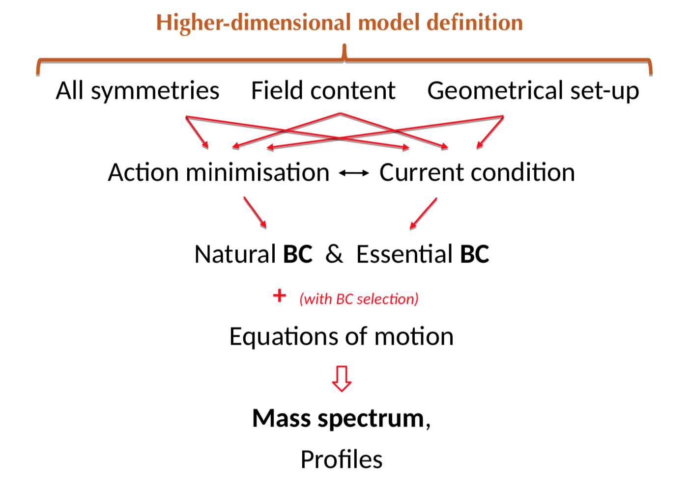
The present study confirms the general methodology depicted in Fig. 4 and presented in Ref. Angelescu:2019viv. Within the present model, the probability current condition on this schematic description is the vanishing of fermion currents at the two fixed points (issued from symmetry criteria and inducing the EBC (57) in the free case). For the interval model, the vanishing current condition is a direct implication of the existence of boundaries for the matter fields. This current vanishing holds both in the presence and absence of brane-localised Yukawa couplings.
In the framework of the orbifold version described in Section 6, the additional field condition (6), coming from the symmetry at the fixed points, accompanies the definition of the symmetry of the bulk action and leads to the new EBC’.
7.2 Discussion of the action content
In addition to the information contained in the action (18), the present orbifold model is defined in a complementary way by other elements like: (i) the junction point at , (ii) the choices of transformations for the fields in the bulk [see Eq. (7)-(10)] and possibly at the fixed points [c.f. Eq. (6)], (iii) the EBC (57) imposed by the model definition when those are used instead of the BBT. Regarding the point (iii), Table 3 summarises the obtained cases where the EBC and the BBT can be used. This table is identical to the one obtained in the interval model study Angelescu:2019viv.
| No boundary characteristic | Vanishing current condition [EBC] | Bilinear brane terms [NBC] | |
|---|---|---|---|
| 4D Approach | (Impossible) | BC () | BC () |
| 5D Approach | (Impossible) | (Impossible) | BC () |
7.3 About the orbifold/interval duality
The present orbifold model and the interval scenario studied in Ref. Angelescu:2019viv are physically different: their geometrical set-ups and Lagrangian symmetries are not identical. Nevertheless, the respective theoretical predictions for the observables like the (brane-coupled) fermion mass spectra and 4D effective Yukawa coupling constants are identical up to factors , which may be called a duality. Indeed, for a comparable dimension size , although the mass absolute values (89) involve a new factor in front of , with respect to the interval analytical result, the measurable range of values for is of the same order and the precise limits of this range rely on the approximate perturbative limits of the 4D effective Yukawa coupling constants proportional to [see Sections 2.2.3 and Eq. (90)-(91)-(92)]. Besides, the dependence of the analytical mass formula on the Lagrangian parameters is identical in the two models, up to this factor entering the coupling constant definition, as can be seen from Eq. (89) and Section 2.2.3 – including the free limiting case . Similar comments hold for the 4D effective Yukawa coupling constants (90) which have additional factors in front of and as an overall factor (latter one induced by normalisation considerations), with respect to the interval case.
The orbifold version of Section 6 contains additional information at the fixed point branes. It predicts thus a specific chirality configuration and mass spectrum [among chiral or vector-like solutions respectively of type ()-()] so that it is not dual to the interval model.
Coming back to the case of duality, there exist similarities between the orbifold and interval models, as it appeared throughout this work when solving the EOM and BC to find out the fields. Let us now comment on the similarities at the Lagrangian level. First, the BBT (17) have the same form as in the interval framework Angelescu:2019viv and the different factor is related to the double size of the compactified space for the identification, . The opposite front sign in the BBT (for a similar profile solution set-up) is just due to a different Dirac matrix sign convention [see sign in Eq. (107)].
In the global action (18), remains to be discussed, the other parts being identical in the orbifold and interval models. Thanks to the orbifold property (2), the change of variable, , allows the following rewriting of Eq. (4),
| (103) | |||||
where the last step is based on Eq. (3). Therefore, using Eq. (18) and the relevant identification, , we can express the orbifold action in terms of the interval action pieces Angelescu:2019viv (indicated by the exponent):
| (104) | |||||
This re-expression reveals an alternative method to derive the fermion masses and couplings, which are independent from the pure scalar part, namely . The idea is that, within the orbifold model now described by the action (104) importantly together with the description of the symmetry over , we can first search for the field parts along the limited domain . This search is in fact based on the action + + + , since the overall factor in Eq. (104) affects neither the EOM (global factor) nor the BC (same factor in front of the surface terms and pure brane terms combined into BC) 2323 23 This search could also be constrained by vanishing currents at instead of the presence, in the free case, as shown in Sections 3.2 and 5.2., and is in turn strictly equivalent to solving the interval model. Given this action, the solutions obtained for the 4D masses (and 4D effective Yukawa coupling constants from profile overlaps with the Higgs boson peak at ) are those of Ref. Angelescu:2019viv but involving a normalised coupling parameter . The last stage of this technics is the extension of the obtained profiles over the complete orbifold domain via the transformations, before applying the ortho-normalisation condition. The 4D effective Yukawa coupling constants are then changed by an additional factor , as is clear from the dimensional wave function normalisation forms (75)-(85), which confirms the result (90). On the other side, we see as well that the fermion masses so obtained (unchanged by the spatial domain extension) involve only a new normalised parameter , with respect to Ref. Angelescu:2019viv, which confirms the found spectrum (89).
Beyond these action correspondences, there are other elegant similarities. For example, as illustrated by Fig. 4, both the interval and orbifold scenarios lead to the same vanishing probability current conditions at the two branes (and hence to identical EBC); those current conditions come, respectively, directly from the interval boundary criteria and indirectly from symmetry considerations. Besides, Table 3 shows that the same treatments of the two branes, at the fixed points or interval boundaries, must be adopted in identical situations and that the same BC are generated.
Finally, let us propose an intuitive description for understanding the orbifold versus interval model duality. The obtained wave functions for the bulk fermions on the interval are of the kind , coming in factor (via the KK decomposition) of the energy coefficients in the 4D Dirac fields, which gives rise to wave planes propagating in both -directions of the interval with momenta – as for oscillations left-moving and right-moving along opposite directions in the world-sheet parameter space of strings. The associated particle, going in the direction and then coming back along , reproduces the propagation along , following consecutively the two fundamental domains and of the orbifold (effectively equivalent orientations of the circle in the bulk so a unique propagation direction chosen along it): exactly the same Lagrangian evolution is felt by this particle during those dual travelings along the extra -dimension, in the two different models, as is clear from the Lagrangian symmetry depicted in the drawing 1.
8 Conclusions
In the study of the orbifold, the proper action definition through improper integrals has allowed to obtain consistent bulk profile solutions with possible discontinuities at the fixed points. In particular the point-like interaction of Yukawa creates a profile jump.
These solutions have been obtained without brane-Higgs regularisation, by relying on the necessary EBC, coming from vanishing fermion probability currents, or alternatively on the introduction of BBT in the action. The associated calculations have been confirmed by the matching, between the 4D and 5D approaches, of the analytical results for the fermion mass spectrum and 4D effective Yukawa coupling constants.
The orbifold version, with transformations of the fields extended to the fixed points, was shown to be able to generate the chiral nature of the theory and even to select the expected SM chirality configuration for the 4D states.
The duality between the interval and orbifold scenarios has been deeply described. It has also constituted the opportunity to point out an alternative method for calculating the tower of excitation masses and 4D Yukawa couplings.
We are now working on the introduction of distributions in this context WIP.
Acknowledgments
R.L. is supported by the agreement signed between the China Scholarship Council (CSC) and the Université Paris-Saclay.
Appendix
Appendix A Notations & conventions
Throughout the paper, we use the conventions of Ref. Schwartz:2013pla. The 5D Minkowski metric is,
where .
The 4D Dirac matrices are taken in the Weyl representation,
| (105) |
where and () are the three Pauli matrices:
One has also the 4D chirality operator,
| (106) |
In our conventions, the 5D Dirac matrices () obey () and read as,
| (107) |
Appendix B From spinor components to compact notations
B.1 Spinor components and their variations
The generic spinor field () introduced via Eq. (6) can be written in terms of its four explicit components []:
| (108) |
and similarly, can be expressed in terms of its own four components :
| (109) |
These 8 components constitute the fundamental variables of the Lagrangian (5). Hence, the variation of the associated Action, [see Eq. (4)], involves the following 8 elementary variations, that we can group into new 4-component (transposed) vectorial objects defined as:
| (110) |
introducing the 8 components and . We then define,
| (111) |
inspired by the following generic relations, based on Eq. (6),
| (112) |
B.2 A typical compact form calculation
B.3 transformations of field variations
Finally, we can derive the transformation for the compact form of Eq. (110). Accordingly to the transformations (7)-(10), we have,
due to the anti-commutator relation . Then one must rewrite this relation by making the spinor components of Eq. (109) appear explicitly:
in order to deduce the relation on the variations of these components:
Thanks to Eq. (110), this equation can be contracted back to the compact notation as,
| (114) |
References
- (1) L. Randall and R. Sundrum, Large Mass Hierarchy from a Small Extra Dimension, Phys. Rev. Lett. 83 (1999) 3370–3373, [hep-ph/9905221].
- (2) S. Chang, J. Hisano, H. Nakano, N. Okada and M. Yamaguchi, Bulk standard model in the Randall-Sundrum background, Phys. Rev. D62 (2000) 084025, [hep-ph/9912498].
- (3) T. Gherghetta and A. Pomarol, Bulk fields and supersymmetry in a slice of AdS, Nucl. Phys. B586 (2000) 141–162, [hep-ph/0003129].
- (4) S. J. Huber and Q. Shafi, Neutrino oscillations and rare processes in models with a small extra dimension, Phys. Lett. B512 (2001) 365–372, [hep-ph/0104293].
- (5) S. Casagrande, F. Goertz, U. Haisch, M. Neubert and T. Pfoh, Flavor physics in the Randall-Sundrum model: I. Theoretical setup and electroweak precision tests, JHEP 10 (2008) 094, [0807.4937].
- (6) S. Chang, C. S. Kim and M. Yamaguchi, Hierarchical mass structure of fermions in warped extra dimension, Phys. Rev. D73 (2006) 033002, [hep-ph/0511099].
- (7) G. Moreau and J. I. Silva-Marcos, Neutrinos in warped extra dimensions, JHEP 01 (2006) 048, [hep-ph/0507145].
- (8) G. Moreau and J. I. Silva-Marcos, Flavor physics of the RS model with KK masses reachable at LHC, JHEP 03 (2006) 090, [hep-ph/0602155].
- (9) C. Bouchart and G. Moreau, The precision electroweak data in warped extra-dimension models, Nucl. Phys. B810 (2009) 66–96, [0807.4461].
- (10) F. Englert and R. Brout, Broken Symmetry and the Mass of Gauge Vector Mesons, Phys. Rev. Lett. 13 (1964) 321–323.
- (11) P. W. Higgs, Broken symmetries, massless particles and gauge fields, Phys. Lett. 12 (1964) 132–133.
- (12) K. R. Dienes, E. Dudas and T. Gherghetta, Neutrino oscillations without neutrino masses or heavy mass scales: A higher dimensional seesaw mechanism, Nucl. Phys. B557 (1999) 25, [hep-ph/9811428].
- (13) A. Abada, P. Dey and G. Moreau, Neutrinos in flat extra dimension: Towards a realistic scenario, JHEP 09 (2007) 006, [hep-ph/0611200].
- (14) Y. Grossman and M. Neubert, Neutrino masses and mixings in nonfactorizable geometry, Phys. Lett. B474 (2000) 361–371, [hep-ph/9912408].
- (15) S. J. Huber and Q. Shafi, Majorana neutrinos in a warped 5-D standard model, Phys. Lett. B544 (2002) 295–306, [hep-ph/0205327].
- (16) G. Moreau, Realistic neutrino masses from multi-brane extensions of the Randall-Sundrum model?, Eur. Phys. J. C40 (2005) 539–554, [hep-ph/0407177].
- (17) J. M. Frère, G. Moreau and E. Nezri, Neutrino mass patterns within the seesaw model from multilocalization along extra dimensions, Phys. Rev. D69 (2004) 033003, [hep-ph/0309218].
- (18) F. Nortier, Large star/rose extra dimension with small leaves/petals, Int. J. Mod. Phys. A 35 (2020) 2050182, [2001.07102].
- (19) F. Ledroit, G. Moreau and J. Morel, Probing RS scenarios of flavour at LHC via leptonic channels, JHEP 09 (2007) 071, [hep-ph/0703262].
- (20) C. Bouchart and G. Moreau, Higgs boson phenomenology and vacuum expectation value shift in the Randall-Sundrum scenario, Phys. Rev. D80 (2009) 095022, [0909.4812].
- (21) A. Djouadi, G. Moreau and F. Richard, Resolving the A(FB)**b puzzle in an extra dimensional model with an extended gauge structure, Nucl. Phys. B 773 (2007) 43–64, [hep-ph/0610173].
- (22) A. Djouadi, G. Moreau and R. K. Singh, Kaluza-Klein excitations of gauge bosons at the LHC, Nucl. Phys. B 797 (2008) 1–26, [0706.4191].
- (23) A. Djouadi and G. Moreau, Higgs production at the LHC in warped extra-dimensional models, Phys. Lett. B660 (2008) 67–71, [0707.3800].
- (24) A. Djouadi, G. Moreau, F. Richard and R. K. Singh, The Forward-backward asymmetry of top quark production at the Tevatron in warped extra dimensional models, Phys. Rev. D 82 (2010) 071702, [0906.0604].
- (25) A. Djouadi, G. Moreau and F. Richard, Forward-backward asymmetries of the bottom and top quarks in warped extra-dimensional models: LHC predictions from the LEP and Tevatron anomalies, Phys. Lett. B 701 (2011) 458–464, [1105.3158].
- (26) A. Angelescu, G. Moreau and F. Richard, Scalar production in association with a Z boson at the LHC and ILC: The mixed Higgs-radion case of warped models, Phys. Rev. D 96 (2017) 015019, [1702.03984].
- (27) C. Bouchart, A. Knochel and G. Moreau, Discriminating 4D supersymmetry from its 5D warped version, Phys. Rev. D 84 (2011) 015016, [1101.0634].
- (28) J. Polchinski, Tasi lectures on D-branes, in Fields, strings and duality. Proceedings, Summer School, Theoretical Advanced Study Institute in Elementary Particle Physics, TASI’96, Boulder, USA, June 2-28, 1996, pp. 293–356, 1996, hep-th/9611050.
- (29) C. P. Bachas, Lectures on D-branes, in Duality and supersymmetric theories. Proceedings, Easter School, Newton Institute, Euroconference, Cambridge, UK, April 7-18, 1997, pp. 414–473, 1998, hep-th/9806199.
- (30) O. Aharony, S. S. Gubser, J. M. Maldacena, H. Ooguri and Y. Oz, Large N field theories, string theory and gravity, Phys. Rept. 323 (2000) 183–386, [hep-th/9905111].
- (31) M. J. Duff, Supermembranes, in 26th British Universities Summer School in Theoretical Elementary Particle Physics (BUSSTEPP 1996) Swansea, Wales, September 3-18, 1996, 1996, hep-th/9611203.
- (32) S. Fichet, Braneworld effective field theories — holography, consistency and conformal effects, JHEP 04 (2020) 016, [1912.12316].
- (33) F. Nortier, Consistency of Braneworld Effective Field Theories, 2007.04266.
- (34) L. J. Dixon, J. A. Harvey, C. Vafa and E. Witten, Strings on Orbifolds, Nucl. Phys. B 261 (1985) 678–686.
- (35) L. J. Dixon, J. A. Harvey, C. Vafa and E. Witten, Strings on Orbifolds. 2., Nucl. Phys. B 274 (1986) 285–314.
- (36) M. Quiros, New ideas in symmetry breaking, in Summer Institute 2002 (SI 2002) Fuji-Yoshida, Japan, August 13-20, 2002, pp. 549–601, 2003, hep-ph/0302189.
- (37) K.-S. Choi and J. E. Kim, Quarks and Leptons From Orbifolded Superstring, vol. 954. Springer, Cham, 2020, 10.1007/978-3-030-54005-0.
- (38) A. Angelescu, R. Leng, G. Moreau and F. Nortier, Beyond brane-Higgs regularization: Clarifying the method and model, Phys. Rev. D 101 (2020) 075048, [1912.12954].
- (39) F. Nortier, Compactified Spacelike Extra Dimension & Brane-Higgs Field, Ph.D. thesis, U. Paris-Saclay, 2020. 2005.00292.
- (40) J. Scherk and J. H. Schwarz, How to Get Masses from Extra Dimensions, Nucl. Phys. B 153 (1979) 61–88.
- (41) E. Cremmer, J. Scherk and J. H. Schwarz, Spontaneously Broken N=8 Supergravity, Phys. Lett. B 84 (1979) 83–86.
- (42) T. Gherghetta and A. Pomarol, A warped supersymmetric standard model, Nucl. Phys. B602 (2001) 3–22, [hep-ph/0012378].
- (43) C. Csaki, C. Grojean, J. Hubisz, Y. Shirman and J. Terning, Fermions on an interval: Quark and lepton masses without a Higgs, Phys. Rev. D 70 (2004) 015012, [hep-ph/0310355].
- (44) A. Azatov, M. Toharia and L. Zhu, Higgs Mediated FCNC’s in Warped Extra Dimensions, Phys. Rev. D 80 (2009) 035016, [0906.1990].
- (45) A. Azatov, O. Bondu, A. Falkowski, M. Felcini, S. Gascon-Shotkin, D. Ghosh et al., Higgs boson production via vector-like top-partner decays: Diphoton or multilepton plus multijets channels at the LHC, Phys. Rev. D 85 (2012) 115022, [1204.0455].
- (46) N. Bonne and G. Moreau, Reproducing the Higgs boson data with vector-like quarks, Phys. Lett. B 717 (2012) 409–419, [1206.3360].
- (47) G. Moreau, Constraining extra-fermion(s) from the Higgs boson data, Phys. Rev. D 87 (2013) 015027, [1210.3977].
- (48) S. Gopalakrishna, T. Mandal, S. Mitra and G. Moreau, LHC Signatures of Warped-space Vectorlike Quarks, JHEP 08 (2014) 079, [1306.2656].
- (49) A. Angelescu, A. Djouadi and G. Moreau, Vector-like top/bottom quark partners and Higgs physics at the LHC, Eur. Phys. J. C 76 (2016) 99, [1510.07527].
- (50) K. Agashe, A. Delgado, M. J. May and R. Sundrum, RS1, custodial isospin and precision tests, JHEP 08 (2003) 050, [hep-ph/0308036].
- (51) M. E. Peskin and D. V. Schroeder, An Introduction to Quantum Field Theory. Addison-Wesley, 1995.
- (52) M. D. Schwartz, Quantum field theory and the Standard Model. Cambridge University Press, 2014.
- (53) R. Barceló, S. Mitra and G. Moreau, On a boundary-localized Higgs boson in 5D theories, Eur. Phys. J. C 75 (2015) 527, [1408.1852].
- (54) Work in progress.