Emergent complex quantum networks in continuous-variables non-Gaussian statesPreprint: APS/123-QED
Abstract
We use complex network theory to study a class of continuous variable quantum states that present both multipartite entanglement and non-Gaussian statistics. We consider the intermediate scale of several dozens of components at which such systems are already hard to characterize. In particular, the states are built from an initial imprinted cluster state created via Gaussian entangling operations according to a complex network structure. We then engender non-Gaussian statistics via multiple photon subtraction operations acting on a single node. We replicate in the quantum regime some of the models that mimic real-world complex networks in order to test their structural properties under local operations. We then go beyond the already known single-mode effects, by studying the emergent network of photon-number correlations via complex networks measures. We analytically prove that the imprinted network structure defines a vicinity of nodes, at a distance of four steps from the photon-subtracted node, in which the emergent network changes due to photon subtraction. Moreover, our numerical analysis shows that the emergent structure is greatly influenced by the structure of the imprinted network. Indeed, while the mean and the variance of the degree and clustering distribution of the emergent network always increase, the higher moments of the distributions are governed by the specific structure of the imprinted network. Finally, we show that the behaviour of nearest neighbours of the subtraction node depends on how they are connected to each other in the imprinted structure.
I Introduction
Large multiparty quantum systems are extremely hard to describe, although the complex behavior of their quantum states is what makes them appealing resources for quantum information processing. Intensive efforts have been dedicated to the direct representation of quantum states via numerical and analytical approaches with the aim of classifying and detecting truly non-classical and useful quantum features, like entanglementIslam et al. 2015; Laflorencie 2016. For example, tensor networks have been demonstrated to be very powerful tools for entanglement classification, and have been applied in many fields ranging from condensed matter physics to conformal field theory Orús 2019. In the quantum information scenario, resource theories offer a general theoretical framework to classify useful resources to reach desired quantum features Chitambar and Gour 2019. Different strategies that are becoming more and more popular exploit machine learning procedures Carleo et al. 2019; Dunjko and Briegel 2018 to classify general complex features in the quantum realm Deng et al. 2017; Carleo and Troyer 2017; Carrasquilla often by representing them via neural networks Guo et al. 2019.

In this work we focus on the complex behaviour of quantum states in continuous variable (CV) quantum systems and we tackle it via complex network theory. Our work is motivated by all-optical platforms, based on continuous quantum observables, that can already produce large entangled networks Asavanant et al. 2019; Larsen et al. 2019; Chen et al. 2014. These networks are made of traveling light fields with quantum correlations between amplitude and phase values of different modes of the field, e.g. light at different colors. They have Gaussian measurement statistics for amplitude and phase continuous variables, so that they can be easily simulated via classical computer. They are essential resources for measurement-based quantum computing but, in order to perform quantum protocols, they must acquire non-Gaussian statistics of the continuous variables. Non-Gaussian statistics can be induced via mode-selective addition and subtraction of photons Ra et al. 2020; Biagi et al. 2020, that are then called non-Gaussian operations. When the number of entangled systems – in our case optical modes – and the number of non-Gaussian operations grow, these systems quickly become hard to benchmark Walschaers et al. 2017a; Zhuang et al. 2018; Albarelli et al. 2018; Takagi and Zhuang 2018; Cimini et al. 2020; Walschaers et al. 2020. Standard quantum optical methods such as homodyne tomography rapidly become intractable, and the properties of the resulting quantum states are hard to unravel.
In the most general scenario, even measurement outcomes of such systems become computationally hard to simulate Chabaud et al. 2017a, so that the associated sampling problem is one of the many variations of bosons sampling Hamilton et al. 2017; Aaronson and Arkhipov 2011. In such sampling problems, photon-number correlations have shown to be efficient tools to extract properties of such intricate systems Walschaers et al. 2016a; Giordani et al. 2018; Phillips et al. 2019; Zhong et al. 2020; Zhong et al. 2021; Madsen et al. 2022. Average values of photon-number correlations can be analytically tractable, but they can only unveil global properties of the system. Yet, to acquire a more detailed image of the state, we can use network theory to analyse distributions of photon-number correlations.
In this work, the use of network theory will be two-fold. First, the optical CV entangled networks can in fact be easily reconfigured in arbitrary shape Cai et al. 2017. We can thus consider entangled networks which are generated through models studied in network theory to reproduce the features of real-world networks. They provide an excellent playground to explore whether mimicking real-world complex network structures Nokkala et al. 2018a; Sansavini and Parigi 2020 provides an advantage for quantum information technologies, including quantum simulation and communication Cai et al. 2017; Arzani et al. 2019 in a future quantum internet. Second, we will use network theory as a powerful tool for benchmarking entangled networks when affected by local non-Gaussian operations by building weighted networks of photon-number correlations. We can then study how different shapes of the initial entangled network can support, enhance, spread or destroy the non-Gaussian features provided by local subtraction of multiple photons.
I.1 Conceptual scheme
The conceptual scheme of our analysis is shown in Fig. 1. Large CV entangled networks have been deterministically implemented via non-linear optical processes. This operation entangles different modes (be they spatial, spectral or temporal) of the fields via an appropriately engineered parametric interaction Roslund et al. 2014; Cai et al. 2017; Chen et al. 2014; Yokoyama et al. 2013; Asavanant et al. 2019; Larsen et al. 2019. These processes are sketched in the left corner of the upper row of Fig. 1, where the different modes are represented by different colors. The circuit representation of the generated states is sketched in the second row of the figure: the non-linear optical process is equivalent to different travelling optical modes occupied by squeezed vacuum states that are entangled via gates. This generates the cluster state Menicucci et al. 2006; Gu et al. 2009. In the third row we show the graphical representation of the state: the different optical modes are represented by different nodes of the network which are linked by gate entangling operations, counted by the entry 1 in the adjacency matrix of the network. This structure is an imprinted network, as it builds the initial quantum states. In the right side of the first column of Fig. 1 we picture the action of multiple-photon subtraction, i.e. the repeated application of the photon annihilation operator on one specific mode of the field. The probabilistic implementation of this operation consists of a mode-selective beam-splitter that sends a small fraction of light to a photon counter: when photons are detected an -photon-subtracted state is heralded. The process can be implemented via non-linear interaction with supplementary gate fields Ra et al. 2020. In the fourth row of the first column we show the network of photon-number correlations between the different field modes that emerge from the imprinted network. This is the emergent network. Its adjacency matrix contains continuous values between and , indicating the strength of photon-number correlations between couple of nodes. In this work we are interested in following the changes of this emergent network of photon number correlations after photon-subtractions on one node as a benchmark of the desired non-Gaussian properties of CV quantum states.
As described above complex networks have a dual role in this work. First, we consider complex network structures for the imprinted network of entangling gates, as shown in the third row of the second column of Fig. 1. We will use complex network models that reproduce particular features of real-world networks. Second, we probe the impact of photon subtraction on the emergent networks by analyzing typical network measures, like degree and clustering, that quantify the number of links and their structure and that are commonly used to characterize complex networks.
I.2 Summary of the results
The entangling -gates in the imprinted network generate short range correlations between nodes. Also, the non-Gaussian operations we consider here - photon-subtractions - are applied locally on a single node. Under such conditions the effect of photon subtraction on a regular graph is limited Walschaers et al. 2018. On the contrary, here we probe imprinted networks constructed from complex network models, where typical distances between nodes are short. Our results are as follows:
- •
The effect of photon-subtraction leads to local changes in the emergent network of photon-number correlations. We analytically prove that the imprinted network structure defines a vicinity of nodes around the photon-subtracted node in which the emergent network changes due to photon subtraction.
- •
For imprinted complex networks we see highly connected emergent networks of photon-number correlations. In such systems we show that photon-subtraction changes the structure of the correlation networks in a profound way in the vicinity of the photon-subtracted node.
- •
We compare different complex network models, like Barabási-Albert or Watts-Strogatz, and their emergent correlation structure before and after subtraction of ten photons. The analysis of the distribution of degrees and clustering coefficients of the emergent correlation networks reveals that the amount of randomness of links or the inhomogeneity of number of links in different network models affects the emergent correlation networks, before and after the photon subtraction. We see that some networks are more efficient than others in spreading the non-Gaussian effect.
- •
For networks in which a majority of nodes is affected by photon subtraction, we show that the global clustering and degree distributions are altered in the same way: the mean and variance increase. This is in contrast with the structure in the tails of the distributions, characterized by higher moments, where the effect of photon subtraction is governed by the specific structure of the imprinted network.
- •
We unveil the importance of the local network structure in the vicinity of the node of photon subtraction. It is the connectivity of the imprinted sub-network spanned by this node and its neighbors that drives the changes due to photon subtraction.
I.3 Structure of the Paper
The Article is outlined as follows. Section II introduces the basic concepts of complex networks and CV cluster states used in this work to make the Article accessible to readers with different backgrounds – readers with one or both areas of expertise may choose to skip this section or particular subsections. We describe the imprinted network structure and review non-Gaussian operations and their importance for getting non-Gaussian CV cluster states. We introduce the emergent correlation networks and complex network measures. Then in Sec. III we look at emergent correlation networks for Gaussian cluster states when different complex network models are used for the imprinted network. This section forms a baseline for the ensuing non-Gaussian analysis. In Sec. IV we describe the evolution of the emergent correlation networks when repeated photon subtractions are applied. We show that photon subtraction in a single node only affects a certain vicinity of the subtraction node. We then analyse the global impact of the non-Gaussian operation on the emergent network. In Sec. V we analyse the local effects of photon subtraction. We show that the sub-networks formed by nodes at different distances from the subtracting point have a different influence on the statistics of the non-Gaussian graphs. We then reveal the driving mechanism for the sub-networks composed by all the node at distance one from the subtracting point , i.e. all the nodes that have a direct link with the subtracting node in the imprinted network. Finally, in Sec. VI we comment on general features of non-Gaussian correlations in photon-subtracted networks and specific features dependent on the imprinted network model.
II Quantum Complex Network theory and Continuous Variable Quantum Systems
II.1 Complex networks and quantum physics
In the last decades, network theory has made significant progress in describing collective features and functionality of complex systems Newman 2018; Barabási 2016. Network-based descriptions are pivotal in social and biological science as well as in technological infrastructures like power grids and information networks such as the internet. The study of complex network structures has spread in physics Albert and Barabási 2002; Dorogovtsev et al. 2008 helping in the description of complex physical systems. Subfields in physics utilizing complex networks include statistical physics, condensed matter and quantum physics with, e.g., the study of the Ising model and Bose Einstein condensation Bianconi 2015; Halu et al. 2013; Jahnke et al. 2008; Burioni et al. 2001; Mülken and Blumen 2011; Valdez et al. 2017; Nokkala et al. 2018b. More recently the study of complex networks has become relevant for quantum systems and procedures employed in quantum information technologies Biamonte et al. 2019; Sansavini and Parigi 2020; Cabot et al. 2018; Nokkala et al. 2018a; Chakraborty et al. 2016; Cuquet and Calsamiglia 2009; Faccin et al. 2014 indicating that a dedicated theory of quantum complex networks needs to be built, especially for networks with no classical equivalent, like those based on quantum correlations or quantum mutual information. In particular, emergent complex networks based on quantum mutual information have determined critical points for quantum phase transitions Valdez et al. 2017; Sundar et al. 2018; Buča et al. 2019. Likewise, complex network theory has been successful in determining self-similarity in entanglement structure of spin-chains Sokolov et al. 2020 as well as new kinds of structured entanglement emerging from quantum cellular automata Hillberry et al. 2020 on qubit/gate/ciruit-based quantum computers. Networks are naturally evoked in the quantum regime in relation to the quantum internet Kimble 2008, where it is not clear yet if the best arrangement of its components will take a complex shape like the classical internet. Networks are however pivotal in all quantum technologies. Indeed, quantum information algorithms and quantum transport can be mapped to quantum walks on regular and complex networks Childs 2009; Mohseni et al. 2008; Plenio and Huelga 2008; Walschaers et al. 2016b. Complex networks have also a crucial role in near-term quantum information processing because they describe networked noisy intermediate-scale quantum computers Awschalom et al. 2019; Altman et al. 2021. Thus complex network theory provides a versatile toolbox, as it can be applied to different quantum features, and is very efficient in revealing emerging collective structural mechanisms.
Here we apply, for the first time, complex network analysis to CV multipartite quantum states. We focus on the ones that can be generated in the more advanced optical platforms, but the method can be applied to general CV states.
Networks are a collection of nodes and links. This is a very versatile conceptual structure that can be applied to any kind of relation between a collection of physical systems: receivers and senders in an information network linked by physical channels; atomic spins interacting via magnetic forces; or physical observables linked by correlation relations. Modern complex network theory in the physical, social, and life sciences is built on graph theory from mathematics and computer science.
The adjacency matrix is the central mathematical object of complex network theory: a non-zero term in the matrix indicates a link between two nodes, where the indices of the matrix determine the nodes. The work done in this Article is based on constructing the adjacency matrices for relevant networks, and subsequently extracting relevant properties from them.
In quantum information, graphs define the structure of the so-called graph or cluster states 11 1 Cluster is sometimes reserved for graphs allowing for universal quantum computing. In this work, however, we use the terms cluster state and graph state as synonyms.. They correspond to multipartite quantum states with a specific entanglement structure introduced in the context of measurement-based quantum computing Raussendorf and Briegel 2001; Raussendorf et al. 2003; Menicucci et al. 2006; Gu et al. 2009. For such cluster states, a non-zero term in the adjacency matrix indicates that an entangling gate has been applied between two qubits or between two quantum fields in two different optical modes (where the information is encoded in discrete or continuous variables, respectively). In this section we first provide a brief introduction to CV quantum optics in II.2 and we review the CV cluster states that are induced by the imprinted networks in Sec. II.3. Then in Sec. II.4 we introduce the photon subtraction operation that creates non-Gaussian features in these quantum states. We define the emergent network of photon-number correlations in Sec. II.5. Finally, in Sec. II.6 we review network measures in the context of complex network models.
II.2 Continuous variable quantum optics
A -mode light field Fabre and Treps 2020 can be described as an ensemble of quantum harmonic oscillators with creation and annihilation operators which obey the commutation relation . In the CV framework, we focus on “position” and “momentum” variables of these harmonic oscillators, and , also called quadratures. Generic quantum states of such quantum harmonic oscillators are hard to characterize, but the subclass of Gaussian states is very well understood. These states are completely described by the quadrature expectation values (the mean field) and covariance matrix . To define the latter, let us introduce the -dimensional vector , and introduce
| (1) |
where denotes the expectation value of the observables in the state . If this state is Gaussian, all its higher order correlations can be expressed in terms of Verbeure 2011 (note that this property is explicitly used in Appendix A).
In this work, we will associate specific optical modes with the nodes of a network, as shown in Fig. 1. Such networks are naturally realized in the cluster state formalism of CV measurement-based quantum computing. It was experimentally demonstrated that such cluster states can be generated in arbitrary shapes Cai et al. 2017.
II.3 Clusters: imprinted quantum networks
In quantum optics ideal cluster states require infinite energy to produce, it is therefor common to consider approximate cluster states, based on applying gates on a set of squeezed vacuum modes. The finitely squeezed states can be written as , where is the squeezing operator, and the vacuum state. The parameter denotes the squeezing, which for simplicity is chosen to be the same in all copies. The unitary gates that entangle these squeezed vacuum modes are given by .
This results in a Gaussian state with covariance matrix (1) given by . The first elements in the diagonal are the variances of the quadrature of the modes (nodes) where is the variance of the quadrature for the vacuum state which is taken equal to 1. The last elements are the variances of the quadrature of the modes. The approximate cluster state that results by acting on with a network of gates is then described by Menicucci et al. 2011 :
| (2) |
Here, is a matrix divided into four blocks. and describe the correlations among the - and -quadratures, respectively, whereas and contain all correlations between - and -quadratures. The presence of in highlights that correlations extend not only between nearest neighbor nodes, but also between next-nearest neighbors of the imprinted network. The elements are in fact known to correspond to the number of walks of exactly two steps from to of the network Gu et al. 2009; Walschaers et al. 2018.
The gates, which create the entanglement, can be implemented according to any network shape, i.e., any adjacency matrix .
When used in measurement-based quantum computing, cluster states are built to ensure persistence of entanglement Briegel and Raussendorf 2001. This means that a measurement on one node only locally affects the state and the surviving entanglement links can be further exploited for the next steps in measurement-based computing. To this end, some regular 2D graph structures, e.g., hexagonal or triangular lattices, have been proven to allow for universal computing. That is, arbitrary unitary operations can be performed via local operations and classical communication on the cluster. In contrast, others have been discarded, e.g. the tree graph Van den Nest et al. 2006.
Here we go beyond such regular structures, motivated by the fact that CV quantum networks in optical setups can be easily reconfigured to arbitrary shapes Cai et al. 2017. We want to indeed replicate in the quantum regime some of the models that mimic real-world complex networks Nokkala et al. 2018a; Sansavini and Parigi 2020 in order to test their structural properties under local operations.
In the remainder of the Article we refer to the network that describes the pattern of gates that are applied to create the Gaussian cluster state as the imprinted network.
II.4 Non-Gaussian operations in continuous variable platforms
Cluster states are characterized by Gaussian statistics of quadrature measurements, which allows for a compact statistical description even when they have a large size. However, for quantum computing protocols, cluster states must also acquire non-Gaussian quadrature statistics via non-Gaussian operations. Unlike the Gaussian case, the quantum features of such non-Gaussian networks are not trivial to classify Walschaers et al. 2017b; Walschaers et al. 2018; Walschaers and Treps 2020. Examples of non-Gaussian operations are the conditional implementation of single-photon subtraction and addition, i.e. the action of
annihilation and creation operators and Ra et al. 2020; Ra et al. 2017; Wenger et al. 2004; Biagi et al. 2020; Parigi et al. 2007; Zavatta et al. 2004; Lvovsky et al..
Such operations have long been investigated as primitive for two important operations for quantum protocols: entanglement distillation and the generation of Wigner negativity.
Single-photon subtraction and addition can also be combined to engender high-order non-Gaussian operations Zhuang et al. 2018; Takagi and Zhuang 2018; Arzani et al. 2017; Yukawa et al. 2013.
In this Article, we focus on multi-photon-subtraction operations that can ideally be represented, in a multimode case, by the following operation on a state :
| (3) |
where denotes a particular mode. In general, Eq. (3) describes repeated subtractions from different nodes, or even from superpositions of different nodes, that have recently been experimentally implemented Ra et al. 2017; Ra et al. 2020. When these operations are applied on multimode quantum states characterization of the resulting states is not a trivial task. Recent results have depicted the rules of thumb for entanglement and Wigner negativity Walschaers et al. 2017b; Walschaers et al. 2017a; Walschaers et al. 2018; Walschaers and Treps 2020, indicating that a deeper structural analysis would be beneficial for a more comprehensive picture.
Here, we specifically consider repeated photon subtractions from one single node of the cluster state in Eq. (II.3). There are two main reasons for this choice. First, we focus on the simplest scheme providing significant statistics. In fact, when multiple subtractions from an arbitrary superposition of nodes are considered, the analysis becomes computationally hard Chabaud et al. 2017a. Second, we aim at probing the extent of the effect of photon subtraction in the most local way possible. In previous work, we have shown that photon subtraction on a given node induces non-Gaussian features in its nearest and next-to-nearest neighbor nodes Walschaers et al. 2018. This Article goes beyond single-point features such as local averages. Instead, we focus on the changes induced in the correlations between those nodes, including beyond next-nearest neighbors. We then study how different imprinted network shapes spread or destroy the non-Gaussian features created by photon subtraction. This is a problem that is very typical for classical information networks, studied here in the new context of quantum correlations.
II.5 Emergent complex networks
of photon number correlations
Covariance matrices are sufficient to explain the behaviour of Gaussian states. In the case of non-Gaussian states expectation values of higher order operators are needed. In this Article, we focus on photon-number correlations, that are simple non-Gaussian observables with a clear physical interpretation. Photon number correlations can be written in terms of quadrature correlations. The expression will then involve fourth moments of quadratures, which are sensitive to the non-Gaussianity – i.e., departure from Gaussian shape – of the quadrature distribution Walschaers et al. 2017a. Moreover, photon-number correlations are extensively used to study features of non-Gaussian processes in quantum optics, such as Hong-Ou-Mandel interference Hong et al. 1987, photon bipartite entanglement Beenakker et al. 2009, and photon distinguishability Walschaers 2020. They also serve to benchmark single-photon sources Somaschi et al. 2016, -photon sources Lachman et al. 2019, and quantum protocols such as boson sampling Walschaers et al. 2016a; Giordani et al. 2018.
To consider structural effects, we introduce a second network for each cluster state, composed by the emergent structure of photon-number correlations between pairs of modes. As such, we define the correlation matrix :
| (4) |
where we take the absolute value of the correlation, since we are purely interested in the strength of the correlation, rather than its sign. The values of depend on the number of photons in the system; it may be higher for two weakly correlated nodes with very high photon numbers, than for strongly correlated nodes with very small photon numbers. Due to its conditional nature, photon subtraction locally changes the photon number in the system, thus making it impossible to genuinely compare the resulting values of in the two cases. The denominator in Eq. (4) solves this problem by renormalizing the correlation to be confined between zero and one, where one implies that both nodes contain the same number of photons, regardless of how many photons there are.
Eq. (4) ultimately allows us to look at the correlation network, as given by its weighted adjacency matrix:
| (5) |
In the following we will characterize what kind of correlation networks () emerge, in the same spirit of mutual information networks in Valdez et al. 2017, when photon-subtraction operations are applied on cluster states with different shapes . Hence, network structures are considered at two different levels: one is the imprinted network which describes the entangling gates that induce Gaussian entanglement between position and momentum in the cluster state of Eq. (II.3); the other is the emergent network of photon-number correlations defined in Eq. (5) via Eq. (4). This second network will be analyzed via measures and metrics typical of complex network theory, as we detail in the following in Sec. II.6.
II.6 Complex network measures
in complex network models
Quantitative measures of network structures have been introduced by network theory Newman 2018; Barabási 2016. From the adjacency matrix components we can calculate the degree for each node , i.e., the number of links connected to it, as
| (6) |
The degree distribution gives the probability for a randomly picked node to have the degree . Even if is not possible to get the full information on the structure of a network by its degree distribution, it can be informative to look at the shape of the distribution. Similarity arguments between different real-world networks have been based in part on analogy between their degree distributions, which often follow a power-law rule. Moreover, many crucial properties of networks, like their robustness to perturbations and the spread of contamination, are determined by the functional Barabási 2016.
A second quantitative measure of complexity is the local clustering coefficient. It gives information on the connections between the neighbors of a specific node, thus keeping track of local correlations around a point. A common way of defining the clustering coefficient is the number of triangles to which the node belongs divided by the number of triplets. It can be recovered from as
| (7) |
for .
Here we briefly review some of the paradigmatic models that have been proposed for real-world networks: the random network model called Erdős-Rényi (ER), the Barabási-Albert (BA) model and the Watts-Strogatz (WS) model. The ER model builds networks by randomly connecting nodes according to a uniformly random probability for two nodes to be connected. The resulting networks exhibit a binomial distribution of links per node. The ER model is able to reproduce the typical average shortest path distances between nodes of real networks.
A second model that has been introduced to reproduce typical complexity signatures of real networks is the BA model. It describes network formation processes based on the preferential attachment model: the network grows by adding new nodes. These new nodes attach with links to old nodes. The probability of connection is proportional to the degrees of the existing nodes, such that the highest degree nodes are the preferred ones. This model is able to reproduce the power-law distribution in the degree, and thus the existence of “hubs”, i.e., nodes with very large degree, as in real-world networks.
Finally, the WS model is able to reproduce the small-world mechanism, where any node is a short path from any other in the network. Specifically, the distance between any two nodes grows as the log of the total number of nodes. It is built by starting from a regular network in which each vertex has a fixed degree ; for instance, would correspond to a lattice in tight binding approximation. Then nodes are rewired according to a probability . One interesting feature of this model is that it allows one to tune continuously from regular () to random () networks.
To achieve reasonable statistics, we consider many realisations of networks made of nodes for each model. For every model we also explore different parameters. These networks are small compared to typical real-world networks, but even for this small scale the different models exhibit visibly different features. In Fig. 3, we show a BA network built by adding new nodes at each step in network growth; a WS network built starting from a regular network with degree per node and rewired with a probability ; and an ER network with connection probability . One observes clear differences between the three networks, with, for example, the emergence of easily visible hubs in the BA model, shown as large blue discs in the figure. By taking network realizations for each model one observes that the resulting degree distribution, shown in Fig. (4), is distinct in the three cases, even if they have similar average value. In particular, the logarithmic scale shows the power-law distribution for the BA networks.
In the following, we choose particular network models to shape the adjacency matrix of the imprinted networks. In the rest of the Article we will consider only the BA and WS models as the ER network shows very similar features as the WS models with high rewiring probability . With the probabilistic generation of a statistically significant number of networks for each model, it will be possible to reveal specific features, in this case quantum ones, that are determined by the structure of the network.
III Emergent networks in complex Gaussian cluster states
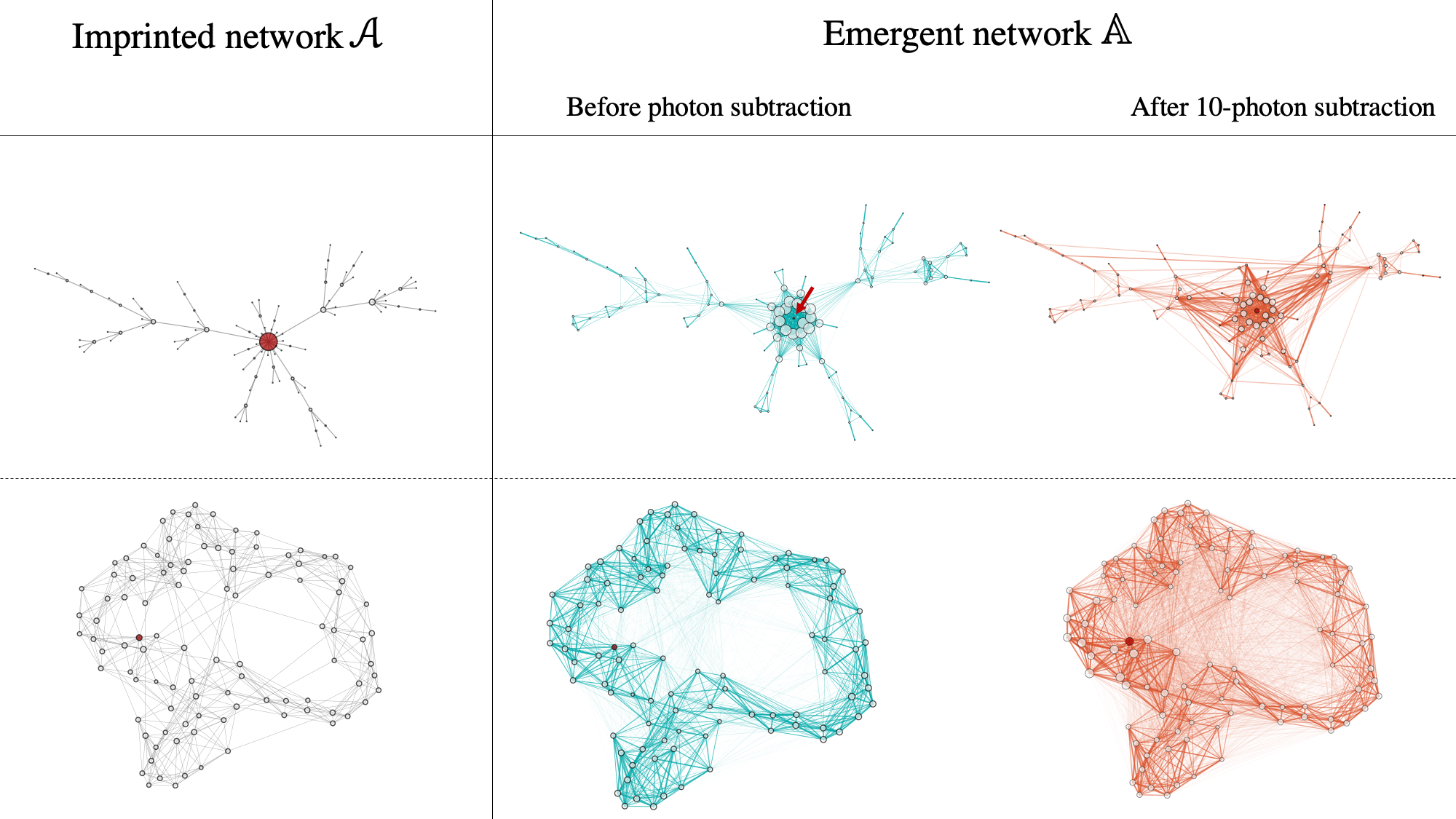
In this section, we explore the emergent photon-number correlation networks for different imprinted networks before any photon subtraction. The quantum state of such networks hence exhibits Gaussian statistics of quadratures. The results of this section form a benchmark to compare with the effect of photon subtraction in Sec. IV and Sec. V.
The imprinted networks are obtained by applying gates to a set of squeezed vacuum modes according to an adjacency matrix for the BA and WS models defined in Sec. II.6. We then examine the emergent network with adjacency matrix . Throughout all our simulations, we fix the amount of squeezing to (i.e., units of shot noise) for each squeezed vacuum mode.
As described in Sec. II.3, the correlation between quadratures of different modes goes beyond the graphical structure imprinted by the gates, as they appear between nearest neighbours but also between next-nearest-neighbors. We then expect photon number correlations to inherit the same behaviour.
The calculation of photon number correlations for the cluster before photon subtraction can be carried out analytically by using the techniques of Appendix A. We obtain the weighted adjacency matrix (as derived in Appendix A.2)
| (8) |
where is a normalization factor depending only on the initial squeezing value and the degree of the node in the imprinted network. Recall from Sec. II.3 that is the number of different walks of exactly two steps that connect nodes and in the imprinted structure. Therefore, as anticipated, the links between nodes and in the emergent network are non-zero if either and are connected in the imprinted network ( = 1) or when they are next-nearest neighbors ().
So emergent networks of photon-number correlations have larger number of links than the imprinted networks. Also, the number of walks of distance two between different nodes in complex networks are larger than in regular structures (like grid shapes). Hence we expect to have a larger number of links for emergent networks of cluster with complex imprinted network.
We now look at specific features dependent on the different network structures.
III.1 Barabási-Albert networks – Emergent triangles and clustering
The imprinted BA networks have a multitude of weakly connected nodes that are organized around a few highly connected hubs.
We collect statistics of different networks of nodes both for the parameter (e.g. top row of Fig. 5) and for . In the example in Fig. 5, we see that the number of links in the emergent network are larger when compared to the imprinted network, as told above. A more quantitative understanding is acquired from the histograms of the degree and clustering coefficients in the emergent network of Fig. 6 for in comparison with the original distribution of the imprinted network. The emergent degree distributions inherit the features of the imprinted network, with a small number of nodes with high degrees, although with larger variances. In contrast, the histogram of clustering is dissimilar to the clustering in the imprinted network. The BA network with is an excellent example to illustrate the difference: this imprinted network’s tree-like structure combined with the randomness of the BA growth process makes that many nodes have only one connection. In the emergent network, however, all nodes have at least two connections due to what we discussed above, i.e., the presence of walks at distances two in the imprinted network. So we have more triangles than in the imprinted network. Thus clustering is zero for all nodes while the emergent correlation network has non-zero values quite uniformly distributed but only in the range of .
III.2 Watts-Strogatz networks –
More randomness for
lower degree and clustering
As mentioned in the introduction to complex networks of Sec. II.6, WS networks have a tuneable degree of randomness. In particular, in the limit of a vanishing rewiring probability we recover a completely regular network, whereas in the limit of high rewiring probability the network closely resembles an ER network. In our simulations, we start from a regular one-dimensional network with nodes, each of which is connected to other nodes. This network can be represented by organizing the nodes in a circle, where every node is connected up to its neighbor. Subsequently we rewire the connections with probability . For various choices of , we implemented of these WS networks as imprinted structures to apply gates 22 2 The case where forms an exception. Here we consider realizations.. As for the BA case we look at the statistics of degree and clustering.
The bottom row of networks in Fig. 5 shows a typical realization of a WS network with and . The imprinted network is therefore reasonably close to a regular network in which each node has connections. We observe that the emergent network before photon subtraction, with a weighted adjacency matrix , has a richer structure in its connections. Nevertheless, we can still see a qualitative resemblance between the imprinted and the emergent network.

In Fig. 7 we examine the difference in degree and clustering coefficient between imprinted and emergent networks. We observe that the properties of the imprinted WS networks strongly influence the structure of the emergent correlation networks. The degree distribution for the imprinted networks is always centered around with larger variances for larger . The degree distributions for the emergent networks are centered around different mean values for the three cases. The case shows a broader and more skewed distribution of significantly higher degrees. Hence, for the emergent networks, in contrast to the imprinted ones, the largest variance is for the lowest . In general, we conclude that an increased probability of rewiring (and thus more randomness) in the imprinted network decreases the degree (which is essentially the total amount of correlation of every node) in the correlation network of Gaussian clusters. The histogram for the clustering coefficient is qualitatively similar to that of the degree, in the sense that increased rewiring leads to a decrease in clustering, and it is also very similar to the clustering of the imprinted networks 33 3 This reduction in the degree and clustering should be explained by a reduction in the weight of the connections because, from (8), we can demonstrate that the number of connection in the emergent network is higher for larger values of . This is related to the choice of the normalization given by the denominator in the elements of the correlation matrix, as explained in Sec. II.5..
IV The effect of non-Gaussian operations on Emergent Networks
In this section we study the effect of photon subtraction, introduced in Sec. II.4, on the emergent network of photon-number correlations. Because the operation is locally applied on a single node in the imprinted network, one might consider this to be a single-node attack, as in classical complex network theory. Moreover in quantum networks, operations like node removal or link shortening have to be introduced in the context of cluster states via Gaussian (homodyne) measurements Gu et al. 2009. However, we emphasize that no nodes are removed in the photon subtraction process. So it is not a single-node attack in the classical sense.
Here we are not interested in modifying the size of the imprinted cluster by removing nodes, but we instead want to analyze the spreading of non-Gaussian correlations in cluster states when affected by photon subtraction in one node. Previous results show that repeated photon subtraction in the same node may increase correlations in the system due to entanglement distillation Navarrete-Benlloch et al. 2012. Also we know that photon subtraction in a given node creates correlations between previously uncorrelated nodes Walschaers et al. 2017b.
However, there is no general result on how the structure of the correlation in the network is influenced by the topology of the imprinted network.
To address this question, we monitor the effect of subtracting ten photons for the emergent photon-correlation networks. Our procedure is the following: i) we first provide analytical results on the reach of the effect of photon subtraction. ii) We then compare the qualitative features that are seen in the histograms of numerically generated distributions of degrees and clustering coefficients. iii) To get a complementary quantitative view, we perform a moment analysis and probe the effect of the non-Gaussian operation on the mean, variance, skewness, and kurtosis. Readers unfamiliar with these quantities can find their definitions in Appendix C. The results of this section will guide the analysis of distance -induced structures in the follwing section V. An overview of the path followed in our network analysis can be found in Fig. 8. In the remainder of the Article we will explain each one of these steps in detail.
The number of photons to be subtracted (ten) is chosen in order to to have a large effect on the emergent network, although we do not find qualitatively different results for somewhat larger or smaller numbers of subtracted photons. However, increasing the amount of squeezing in the initial imprinted network or the number of photon subtractions does quantitatively enhance the observed features.
IV.1 The effect of photon subtraction is strictly local
The subtraction of a single photon in a cluster state is known to only affect vertices in the vicinity of the node of subtraction Walschaers et al. 2018. In Appendix B, we extend this understanding to the correlations between observables that are defined on different regions of the system: the correlation between two observables and can only be influenced by photon subtraction when both observables have a support on modes that are correlated to the mode of photon subtraction. This result applies regardless of the number of photons that are subtracted.
For the networks in this work, we subtract photons in one specific node. In the initial Gaussian state, Eq. (II.3) shows that this node is correlated to all nodes that are either nearest-neighbours (given by ) or next-to-nearest neighbours (given by ) in the imprinted network of gates. We label the node of photon subtraction and denote the expectation value in the photon subtracted state , whereas is the expectation value in the Gaussian cluster state. Our general result of Appendix B then shows that for all nodes and which satisfy the condition that either or . More colloquially phrased, photon subtraction in only alters the value of if either node or node is a nearest or next-to-nearest neighbour of in the imprinted network.
Looking back at Eq. (4), we must also consider the effect of photon subtraction on the denominator on the final emergent network. Let us assume that node is within the vicinity of , i.e., , but is further away, i.e., . In this case, after photon subtraction in we obtain the Gaussian value when we calculate . Likewise, we will find that remains unaffected. However, because is in the vicinity of , we do find that changes its value. In other words, photon subtraction will still have an effect on the emergent network as constructed via Eq. (4), unless . From Eq. (8), we see that this implies that the effects of photon subtraction spread up to four steps in the emergent correlation network.

We therefore have proven that effects of photon subtraction in such a multimode system can only affect a certain environment around the node of subtraction. Moreover, the number of nodes, in which the effect of photon subtraction is felt, is independent of the number of subtracted photons. Hence, to study the effect of photon subtraction, we can restrict ourselves to intermediate network sizes, that have a large fraction of the nodes that lie in the vicinity of the photon-subtracted node.
Figs. 9 and 10 show how the size of these neighborhoods increases with the size of the network. In almost all cases we consider, we find that this growth either stops or stagnates when the size of the neighborhoods reaches around 100 nodes. The notable exception is the case of BA networks when we subtract a photon in the most highly connected node. This observation is consistent with the fact that BA networks can have very high connectivities, as is also shown by the power-law statistics in 4.
Note that for WS networks the size of the vicinity of the photon-subtracted node could also be changed by increasing or decreasing the connectivity of the initial regular network that is rewired. However, throughout our text we choose to keep it constant at . As such, for the types of networks and the parameter ranges we consider a choice of nodes guarantees that most correlations in the system are affected by photon subtraction in a single node.

As we will show, the methods of complex network theory offer a new window to understand how photon subtraction influences the correlations in the relevant range.
We also arrive at another important conclusion: to induce non-Gaussian effects in vast cluster states, one must subtract photons in many different nodes. However, in Appendix A.3, we argue how the complexity of this problem effectively makes it computationally hard to simulate. From a physical point of view, one would subtract these photons by coupling a tiny amount of light from the subtracting nodes, into an auxiliary mode. Then we need photon detectors on these auxiliary modes to fire at the same time. We can notice the connections to Gaussian boson sampling Hamilton et al. 2017; Gagatsos and Guha 2019, where it is shown that simulating the clicks of photon detectors mounted on a sufficiently complicated Gaussian states is computationally intractable. Similarly, there is also a direct connection to the hardness of sampling continuous variables on a photon subtracted state Chabaud et al. 2017b.
On a mathematical level, the problem at the basis of the computational complexity of these sampling problems is finding perfect matchings Deshpande et al. 2021. As we argue in detail in Appendix A.3, the problem of finding all perfect matchings also appears when constructing the emergent network of photon-number correlations. Hence, fully simulating such networks in detail is only possible when many photons are subtracted in many modes.
Yet, when large states with photons subtracted in various modes are created in experiments, the measurement and analysis of emergent correlation networks may well turn out to be an important tool to characterise such states. Note that the same type of photon-number correlations have been used to benchmark computationally intractable Gaussian boson sampling experiments Zhong et al. 2020; Zhong et al. 2021.

IV.2 Photon subtraction in Watts-Strogatz networks – More randomness for larger effects
Fig. 9 suggests that we can maximize the effect of photon subtraction by subtracting the photons in the node with the highest connectivity in the imprinted network, i.e., the biggest hub. As such we probe network environments in the imprinted WS structure with the highest correlations. For the considered network size of 100 nodes, this choice has a small effect in the case of WS networks as most nodes have a similar connectivity, unlike BA networks where a few nodes serve as highly connected hubs.
In Fig. 11 we choose rewiring probabilities , as for the Gaussian case, to probe the effect of different imprinted network environments on the degree distribution in the emergent network of photon-number correlations. The data for each value of are obtained by combining random realizations of a -node network.
The effect of photon subtraction is qualitatively similar in all cases. A subset of nodes in the photon-subtracted cluster states retains degrees of the same order of magnitude as for the Gaussian network state, whereas a second subset finds its degree considerably increased, resulting in a bimodal distribution. This qualitative similarity translates to the moments in Fig. 11(B), in the sense that photon subtraction shifts the distributions to higher means and variances, regardless of the value of . However, photon subtraction causes stronger increases in the mean and variance for larger values of , and the higher moments behave differently depending on . These features are observed in Fig. 11, where an increase in lowers the overlaps between the histogram before and after photon subtraction.

In Fig. 12, we explore the role of photon subtraction on the clustering coefficients. The observed difference between different values of is even more profound: the clustering coefficients are only weakly affected by photon subtraction for , whereas for the histogram changes dramatically. These drastic changes are also seen when comparing the moments before and after photon subtraction in Fig. 12 B, where photon subtraction increases the skewness and kurtosis for , but strongly decreases these moments for . Nevertheless, even though the clustering coefficients are not strongly affected by photon subtraction in imprinted WS structures with , these clustering coefficients remain much higher than those of the imprinted networks with higher values of (which one can also confirm in the moments).
These observations coincide with the intuition that photon subtraction generally increases the correlations in our system. However, it remains to understand which features of the network structure associated with the different values of determine the extent of the effect of photon subtraction.
In Fig. 13 we compare the effect of photon subtraction on WS networks with and for different network sizes. In this particular case, we compare the histograms for the degrees and clustering coefficients obtained from 100 networks of 100 nodes to those for 10 networks of 1000 nodes. To limit computational times, the node for photon subtraction was chosen randomly (rather than the one with the highest connectivity). As can be deduced from Fig. 9, the fraction of nodes in the network that is in the vicinity of the photon-subtracted node decreases with the size of the network. This leads to a sort of dilution of the effect of photon subtraction when we study global properties of the emergent correlation networks. This is clearly seen, both in the degree distribution and in the distribution of clustering coefficients.
The behaviour in Fig. 13 is a manifestation of the limited size of the vicinity of the photon-subtracted node as compared to the global network. From Fig. 9, we see that this behaviour can be be observed in all considered cases. As long as we subtract all photons in the same mode, there is not much to be gained from increasing the system size beyond 100 nodes. Instead, it is much more interesting to try and understand the local properties of the emergent networks, i.e., what is happening in the vicinity of the photon-subtracted node. This analysis will be presented in Section V. First, however, we will explore how the characteristics of emergent correlation networks are globally affected for BA imprinted structures, where the imprinted networks have a very different degree distribution.

IV.3 Photon subtraction in Barabási-Albert networks –Difference between random and highly connected subtraction node
We now explore how photon subtraction affects the emergent network of a BA imprinted structure, both when we subtract always from the most important hub (i.e., the node with the highest connectivity in the imprinted network), and when we subtract in a randomly chosen node (likely a node with low connectivity).


Even before photon subtraction the moment analysis in Fig. 14(B) shows that for imprinted BA structures the degree distributions of emergent correlation networks have a large variance and kurtosis, in particular for . Hence, the emergent networks inherit some of the power-law features of the imprinted structures. In the top panels of Fig. 14 we therefore show the degree distribution on a log-log scale, for and , before and after subtraction of ten photons.
For imprinted structures, the effect of photon subtraction manifests within the tail of the distribution. We observe the power-law behaviour that is suggested by the moments, and we find that photon subtraction in a hub tends to reduce the weight in the tail. Thus, photon subtraction in the most important hub has a reasonably small effect on a large fraction of the network to make the degrees somewhat more homogeneous. In contrast, photon subtraction increases the weight in the tail if it occurs in a randomly picked node. This shows that, when the photons are subtracted in a node that is correlated to only a small number of other nodes, it can very significantly increase these correlations, thus causing larger values to appear in the tails. This behaviour is consistent with photon subtraction as a finite resource for entanglement distillation. Yet, it must me stressed that photon-number correlation are not necessarily quantum correlations. For nodes with a high connectivity, photon subtraction only weakly alters the individual correlations. As a final comment for the case, we must note that the bulk of the distribution remains largely unaffected, up to a point where the effect of photon subtraction is hardly visible when the histogram is plotted on a linear scale – this is also reflected by a relatively small change in the mean degree.
For imprinted structures, the distribution does not show typical power-law behaviour, which is reflected in smaller values of kurtosis in Fig. 14(B). These moments, nevertheless, show a profound change in the variance due to photon subtraction, which implies an overall widening of the distribution. Figure 14(A) shows this feature, as now a larger fraction of the distribution grows to higher values of the degree. Hence, for we can conclude that photon subtraction predominantly affects the bulk of the distribution, which is qualitatively similar to what we saw for WS distributions.


In Fig. 15 we observe that for the clustering coefficients in these networks can be increased up to , though only for a small fraction of nodes. In other words, photon subtraction, again, predominantly affects the tails of the distribution for (which is confirmed by the moment analysis in Panel B of Fig. 15). Therefore random tree networks (i.e., BA with ) globally seem to be the most resilient networks to local photon subtraction operations, even though photon subtraction in nodes with few links can cause profound local changes in the correlations. For we again see a larger overall impact of photon subtraction, leading to more significant changes to the bulk of the distribution. This, too, is in line with the degree statistics.
These results suggest that the environment of the subtracted node in the imprinted network plays an important role in how the emergent network reacts to photon subtraction. To unravel this interplay between the imprinted structure and the emergent network, we will investigate the behaviour of nodes depending on their distance (in the imprinted network) to the node of photon subtraction.
Note that the power-law degree distribution of the imprinted networks can lead to very large vicinities of the photon-subtracted nodes (in particular when we subtract photons in a hub). This means that the number of non-Gaussian correlations in the networks can rapidly grow, as shown in Fig. 10. In our present implementation of the code to simulate the correlation networks Walschaers 2021, this makes BA networks beyond 100 nodes numerically very challenging to treat.

V Imprinted structure guides non-Gaussian effects
The results in Section IV.1 and the more general theorem presented in Appendix B show that the study of the non-Gaussian correlations induced by photon subtraction is actually a study of sub-networks rather than the study of the global state, as it was shown in Fig. 13. In this section we go beyond the simple separation of affected (i.e. the vicinity of the photon-subtracted node) and unaffected nodes, and explore more detailed sub-structures of the networks.
In Subsection V.1, we first explore how distances for the photon-subtracted node in the imprinted network have an effect on the emergent correlations. This will notably highlight a different behaviour for nearest and next-to-nearest neighbours. In Subsection V.2, we will then explore in detail how the structure nearest-neighbour sub-networks of the imprinted networks have a profound influence of the non-Gaussian effects that manifest in the photon-number correlations.
V.1 Distance-induced structure
In Sec. IV, we showed that photon subtraction induces additional structure in the emergent network.
Here, we take the first step toward understanding how the emergent structure in photon-number correlations is influenced by the imprinted structure. We break up the statistics according to the imprinted distance between the node in which the photons were subtracted and the nodes under consideration. This distance between nodes is here understood to be the number of connections in the shortest path that connects the nodes in the imprinted structure.
In Sec. IV.1 we emphasised that the quantity is only altered by photon subtraction when nodes and are both in the vicinity of the point of photon subtraction. When at least one of the vertices lies beyond, the features of its emergent correlations are only impacted via the denominator in Eq. (4). For the degree statistics, this means that nodes at distances zero (point of subtraction), one (nearest neighbours), and two (next-to-nearest neighbours) are very differently affected by photon subtraction than the remaining nodes. This motivates the choice to separate the nodes into four groups: the nodes where the photons are subtracted (distance 0); their nearest neighbors (distance 1); the next-nearest neighbors (distance 2); and all the remaining nodes (distance 3 or more).


As an example of such a distance analysis, in Fig. 16 we show four histograms corresponding to our four chosen groups of nodes. A complementary quantitative view can be obtained by studying the moments of these distance-resolved histograms, as shown in the moments of the degree distribution in Fig. 17 for imprinted WS structures and in Fig. 18 for imprinted BA network. A completely analogous analysis can be carried out for the clustering coefficients.
The moments in Figs. 17 and 18 provide a range of important insights. First, we find that degree distribution of nodes that lie beyond the next-nearest neighbors () are generally unaltered by photon subtraction. A notable exception is found for the imprinted BA network with photon subtraction in a random node, where the higher moments, i.e., skewness and kurtosis, for these nodes are influenced. This is consistent with the idea that, for an imprinted BA network with photon subtraction in a random node, the non-Gaussian effects are confined to a smaller number of nodes, which in turn change more drastically.
As a second observation, we find that the distance-dependent effects in the skewness and kurtosis depend strongly on the specific network-type and chosen parameters, in contrast to the mean and variance. This implies that photon subtraction induces some general effects on the bulk of degree distributions (as comprised by the first two moments), while the effect on the finer structure (as comprised by the higher moments) of the degree distributions depends more strongly on the precise topology of the imprinted networks.
As an important general effect, we find that both for the nodes in which photons are subtracted (0) and their next-nearest neighbors (2) the mean and variance of the degree distribution always increase. The behaviour of the nearest neighbors (1) is less systematic. For imprinted BA networks with photon subtraction in a random vertex, the mean and variance are essentially unaltered for the nearest neighbors. In contrast, for imprinted WS networks, and the BA network with photon subtraction in the node with highest connectivity, the mean and variance increase for these nodes. For the imprinted BA network with and photon subtraction in the node with highest connectivity, we find that the mean and variance decrease after photon subtraction. Hence, there must be other features in the topology of the imprinted network that influence the degree distribution of the nearest neighbors. These features will be laid out in the following subsection.
V.2 Nearest-neighbors (1) subnetworks

In Fig. 19 we show that the effect on the degree of a nearest-neighbor node in the emergent correlation network is influenced by the number of other nearest neighbors it is connected to in the imprinted networks. This highlights the importance of the topology of the distance-1 sub-network, as compared to the total imprinted network. Quantitatively, this connectivity can be obtained by analyzing the nearest-neighbor sub-network, as highlighted in Fig. 20. When we analyze all the nearest-neighbor sub-networks of our simulated WS networks, we obtain the result in Fig. 19. The bottom row of figures clearly shows that the degrees (in the emergent network) of nearest neighbors are more strongly affected by photon subtraction when these nodes have a higher number of connections to other nearest neighbors. Thus, the different shapes of the nearest neighbor distributions (1), for different values of the rewiring probability , can be fully understood from the nearest neighbor sub-network in the imprinted structure.
We note that photon subtraction shifts the histograms which group nearest-neighbor nodes according to their connectivity in the distance-1 sub-network to higher mean values for higher connectivity. However, for nodes that are not connected to other nearest neighbors, we witness a slight decrease in the average degree due to photon subtraction.
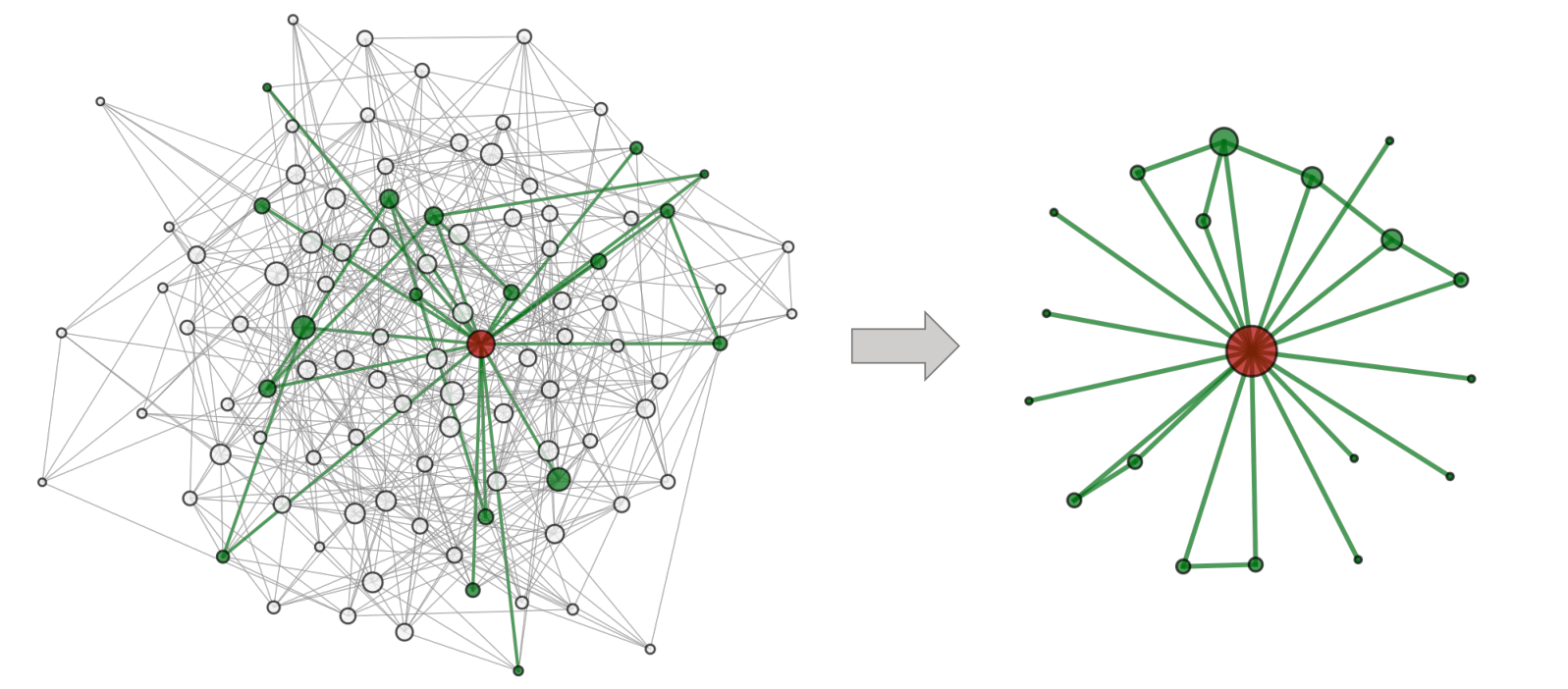
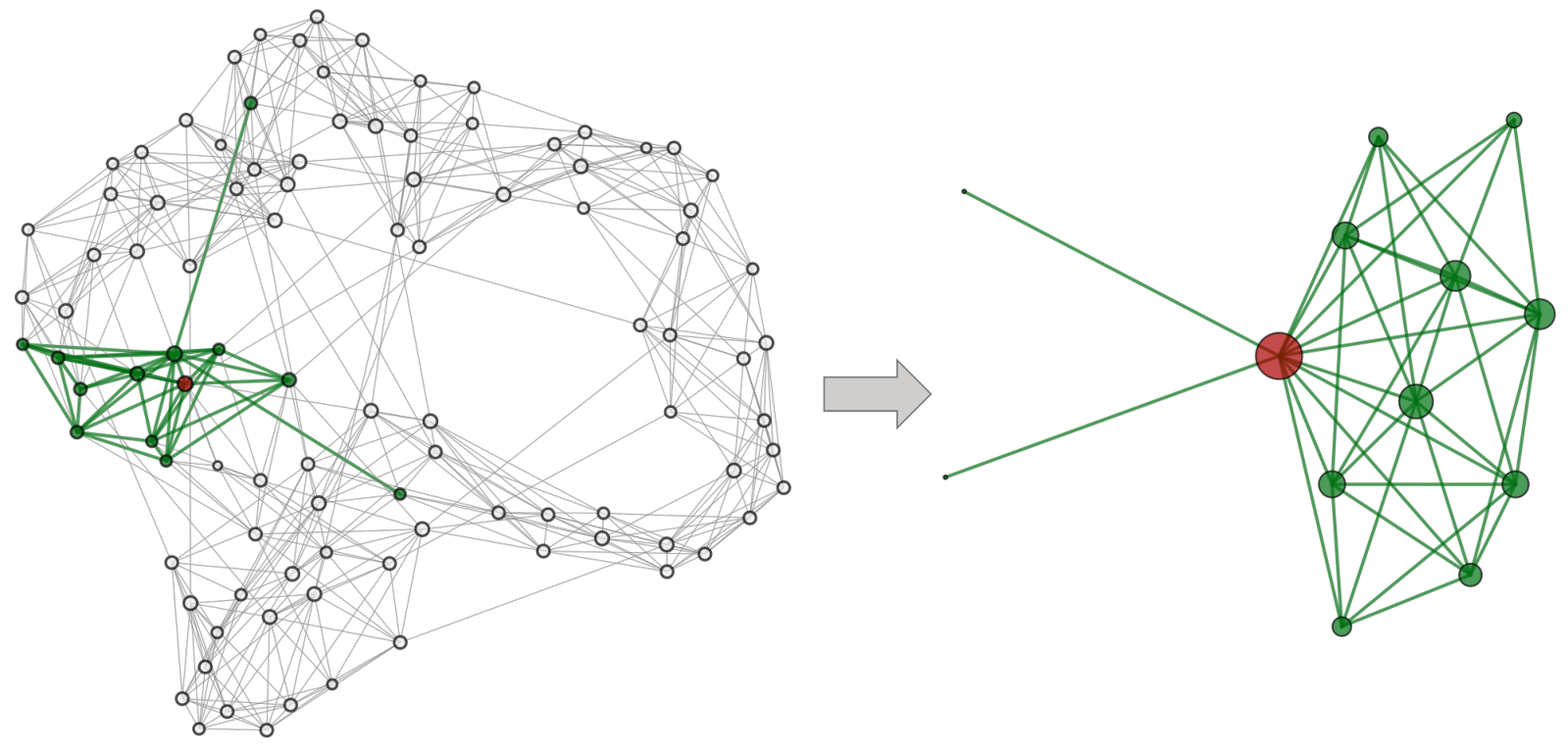
For in Fig. 20, we observe a significant fraction of nearest neighbors that are not connected to any other nearest neighbors. This provides a sharp contrast with the case for , where we observe that networks tend to form clusters, such that nearest neighbors are more likely to be connected to each other. From Fig. 19, we can understand how these features of the imprinted structure have a direct effect on the statistical features of the emergent network.
Similar analyses have been carried out for the nearest neighbor networks of all simulated classes of networks, leading to the same results. A particularly striking case is the BA network with : because these networks are tree-like, nearest neighbors are never connected to one another. This explains why in Fig. 18, for , the means for nearest neighbors (1) are reduced by photon subtraction. Moreover, we can now explain why in Fig. 18 the contribution of the nearest-neighbor sub-network for photon subtraction from the highest degree node for BA with is more important than in the case of subtraction from a random node. In this latter case it is more likely to select one of the isolated nodes with a surrounding nearest-neighbor sub-network also characterized by low connectivity. However, the analysis is not sufficient to explain why the next-to-nearest neighbors (2) are so strongly affected by photon subtraction from a random node in the BA network with .
VI Summary, Discussion, and Outlook
We have addressed the question of how emergent complexity arises from imprinted complexity in continuous variable (CV) quantum networks. In particular, we have studied how localized non-Gaussian features, a key feature of CV quantum technologies and quantum networks such as a future quantum internet, spread through emergent network correlations. Specifically, we used tools from complex network theory to analyze emergent networks of photon-number correlations that manifest in CV cluster states. These cluster states were initially taken as Gaussian states, constructed by applying an imprinted network of entangling gates to a series of squeezed vacuum modes; non-Gaussian states were then created via photon subtraction. We focused on the particular case in which these imprinted networks of quantum gates were chosen to have a complex network structure, implementing either a Watts-Strogatz (WS) or Barabási-Albert (BA) model.
For Gaussian states created by imprinting WS networks, we found that increased probability of rewiring (and thus more randomness) in the imprinted networks decreases the typical degree and clustering coefficient in the emergent correlation network. When BA structures were imprinted, we found that emergent correlation networks inherit heavy tails with a structure that is strongly influenced by the number of connections added with every node in the BA preferential attachment process. For tree networks (), the emergent networks were found to inherit a power-law tail in its degree statistics. In contrast, this power-law behavior was not observed for .
We rendered the states non-Gaussian by subtracting ten photons in a specific node of the system. The short distance between the different nodes in the network guaranteed that the effect of photon subtraction spread far throughout the state. We showed that network theory methods are well suited to characterize the resulting non-Gaussian states, as photon subtraction was found to profoundly change the structure of the emergent networks (see Fig. 5 for an example). We quantified this effect by comparing the distributions of the degrees and clustering coefficients before and after photon subtraction. Generally, we found that photon subtraction increased the typical degree and clustering coefficient, as seen from the mean, and increased the spread of these quantities as characterized by a growing variance. However, we also observed that the higher moments, and thus the finer structure in the tails of the distributions, depended more strongly on the network types and chosen parameters. For BA imprinted networks, we found a strong variation in behaviour of the emergent correlation network depending on whether the photons are subtracted from a hub or a random node. This highlights the importance of the local network topology in the vicinity of the node of photon-subtraction.
We proceeded to dissect the structure of the emergent correlation networks, based on the features of the imprinted network. As a first step, in Sec. V.1, we filtered nodes in the emergent network based on their distance to the node of photon subtraction in the imprinted network. Generally, we found that photon subtraction increases the variance and mean in the nodes of photon subtraction (distance 0), as well as for next-nearest neighbors (distance 2), while the first two moments of nodes that were further removed (distance ) remained unaffected. However, the nearest neighbors (distance 1) in imprinted tree networks defied this global trend. In Sec. V.2 we showed this is due to the particular structure of the nearest-neighbor sub-networks that are extracted from the imprinted network. When we further filtered the nodes at distance 1 based on their connectivity to other nodes at distance 1, we found that higher connectivity led to a stronger increase in the typical degree due to photon subtraction. In other words, nearest-neighbor nodes were more strongly affected by photon subtraction if they were connected to many other nearest-neighbour nodes. In a tree network, nearest neighbours can never be connected to other nearest neighbors, which slightly decreased the average degree in the correlation network for the nodes at distance 1. The distance-resolved moment analysis furthermore showed that the fine structure in the tails of the distributions, as captured by higher moments, does depend strongly on the network topology.
The structural features we uncovered help us understand that the bulk features of emergent correlation networks of imprinted tree structures are only slightly impacted by photon subtraction. The effects that do manifest are mainly observed in the tails of the distribution, as seen in the moment analysis. The difference between subtraction in a random vs. a highly connected node is particularly interesting when interpreted in the light of the network structure. Photon subtraction is a finite resource to enhance correlations in the system. On the one hand, in a node that is correlated to only a small number of other nodes it significantly increases correlations between this small set of nodes, thus causing larger values to appear in the tails. On the other hand, when a photon is subtracted in a hub with very high number of nodes correlated to it, the increase in correlations is spread out.
This work represents a first test of complex network structures in the CV quantum regime under the applications of necessary non-Gaussian operations. We believe this investigation can be fruitful for making decisions about the structure of future quantum technologies on a large scale.
We want to stress that the network models we have chosen are a very limited set of the ones that have been developed in complex network theory. The ones we selected have specific features - in particular: variable level of randomness, presence of hubs, power law distribution, and average short path distances - that have never been tested before in non-Gaussian cluster states. Of course other models and features can be treated in future works.
Moreover, complex network methods have proven useful for the theoretical investigation of such classes of states. Indeed, the characterization of highly multimode non-Gaussian states is generally an arduous task, where standard tools of CV quantum optics fall short. Typical experimental methods such as homodyne tomography lack the necessary scaling properties to study these systems, and theoretical constructs such as Wigner functions become hard to handle. To overcome this problem, one may look for global properties, e.g., Wigner negativity of the full multimode states Cimini et al. 2020. Such global features have the disadvantage that they gloss over the local or neighborhood structures of the state, which are essential in multi-partite quantum platforms. Our results show that network theory offers effective statistical tools for studying these states. At present, we are unaware of any other method that allows us to describe the physical features that we deduced for these large non-Gaussian states. They offer us a road map for more detailed bottom-up studies of particular features such as the role of connections in the nearest-neighbor sub-network.
Acknowledgements.
This work was supported by the European Research Council under the Consolidator Grant COQCOoN (Grant No. 820079). This work was also performed in part with support by the U.S. National Science Foundation under grants CCF-1839232, OAC-1740130, PHY-1806372, and PHY-1748958; and in conjunction with the QSUM program, which is supported by the Engineering and Physical Sciences Research Council grant EP/P01058X/1. We thank the Complex Quantum Systems group at Laboratoire Kastler Brossel (and in particular D. Delande) for access to their computational facilities. The software used to generate the complex networks in the Article is available on Walschaers 2021Appendix A Simulating cluster states and the evaluation of photon-number correlations
A.1 Perfect matching
To execute the simulations presented in this article, we generated random complex networks using the “python-inetwork” library. From these randomly generated networks, we extracted the adjacency matrix to generate the cluster state covariance matrices, as described in Eq. (II.3). After generating the covariance matrix of a Gaussian network state, we used it to evaluate the photon-number correlations of Eq. (4) for the photon-subtracted states in Eq. (3).
The main technique used to evaluate these correlations relies on the properties of Gaussian quantum states. We previously used this method to fully characterize single-photon subtracted states in Walschaers et al. 2017a. We illustrate this method by highlighting the evaluation of the element in Eq. (4). For a photon-subtracted state we find
| (9) |
where denotes the density matrix of the Gaussian network state and . We then use a general property for Gaussian states, that allows us to express
| (10) | ||||
where we introduce the label to denote a “perfect matching.” A perfect matching means any way of dividing a set up into pairs, while maintaining the order. When we consider, for example the set , one possible perfect matching would be . In this example, the notation refers to and . In Eq. (10), these perfect matchings are used to split the set of creation and annihilation operators, , in pairs: In total, we have creation and annihilation operators, which we can associate with a set of indices . The sum over runs over all possible perfect matchings of this index set. For every given perfect matching , we then multiply all the quantities for the different paired indices . The quantities and are indices in the index set, and the quantity denotes the creation or annihilation operator that occurs at the th position in the product . Let us list some examples: , , and .
What remains is now to evaluate the quantities , and this can be done directly via the covariance matrix , by expressing the creation and annihilation operators in terms of quadrature operators (see also Walschaers et al. 2017a; Phillips et al. 2019 for more details). We find the following identities:
| (11) | ||||
| (12) | ||||
| (13) |
These identities are expressed in the mode basis that corresponds to the nodes of the network state.
Using Eqs. (II.3) and (11)-(13), we can calculate the weighted adjacency matrix of the emergent network, . In principle, it is possible to calculate for both the cluster state as well as the photon-subtracted state. However, as we will show, it is exponentially difficult to write a closed-form expression for in the photon-subtracted state. Below, we will first calculate in the cluster state. Then we discuss the photon-subtracted case.
A.2 Gaussian state
Since the cluster state is Gaussian, one can evaluate the connected correlation by applying Eq. (10). Only two terms remain, giving
| (14) |
Each term on the right hand side of Eq. (14) can be evaluated using Eqs. (II.3) and (11)-(13).
For , we have
| (15) |
Therefore
| (16) |
where we used that .
A.3 Photon-subtracted states
For photon-subtracted states, the correlations quickly become hard to evaluate. At the basis of this complexity lies the appearance of perfect matchings in Eq. (10). Finding all possible perfect matchings is a computationally hard problem that belongs to the complexity class . It is also the problem which lies at the basis of the hardness of Gaussian Boson Sampling. Hence, when the number of subtracted photons grows, correlation functions quickly become practically impossible to evaluate.
Generally speaking, the best algorithms for evaluating Eq. (10) use recursive techniques. In our work, we greatly simplify this computational problem by subtracting all the photons in the same mode, i.e., . In this case, expression (9) for only contains creation and annihilation operators in three different modes. This greatly limits the different possible factors that can appear in Eq. (10). Many different partitions will lead to equivalent contributions. The problem thus reduces to that of identifying all the different classes of partitions, evaluating the contribution, and counting the multiplicity.
Once we subtract more than three photons, the total number of different classes of terms remains fixed. We evaluated these by hand and counted a total of 43 classes, each appearing with a certain multiplicity. The correlation networks are then calculated by evaluating the contribution by multiplying relevant quantities given by Eqs. (11) - (13) for each of these 43 classes. Then we multiply each contribution with the right multiplicity, which depends on the number of subtractions and can be calculated through combinatorics. The quantities are evaluated using the same method. For more details, we refer to the code that was used to carry out the simulations Walschaers 2021.
In Appendix B, we prove analytically that the photon number correlations only change when nodes and are in the vicinity of of the photon-subtracted node (see Appendix B for details). This implies that we can first generate a full correlation network of Gaussian correlations by relying on the analytical formula (16) and subsequently we can use (10) to update only the affected correlations. This method is implemented in the second version of our code for simulating WS networks Walschaers 2021.
Appendix B Correlations unaffected by photon subtraction
In this section of the appendix, we prove a general result for correlations in -photon subtracted states: photon subtraction can only change the covariance between observables, if both observables are initially correlated to the mode in which the photons are subtracted.
Assume that we subtract photons from Gaussian state in a mode with label and associated annihilation operator . We denote the algebra of observables as those observables which are “near to ” in the sense that is generated by observables and for which either or . Following Eqs. (11)-(13) we can equivalently define as the algebra of observables restricted to the modes with labels for which the matrix
| (19) |
We then define as the complement of in the sense that , where is the full algebra of observables on the -mode Fock space that describes the entire system.
Theorem B.1.
For any observable and another arbitrary observable , it holds that
| (20) |
where denotes the expectation value in the -photon subtracted state and is the expectation value in the initial Gaussian state.
Proof.
We first of all use that every observable can be arbitrarily well approximated by a polynomial in creation and annihilation operators in . This implies that
| (21) |
where can either be a creation or an annihilation operator. The sum over takes into account that there are many possible products of creation and annihilation operators, also known as Wick monomials, of length . And similarly for we find
| (22) |
To highlight that the creation and annihilation operators that build and have different supports, we have noted the the creation and annihilation operators for as .
The fact that any observable can be written as a series expansion of creation and annihilation operators implies that our theorem can be proven by proving that
| (23) |
First of all, let us consider the term
| (24) |
Because , we find that and . An application of Eq.(10) than shows that
| (25) |
When we then take into account the denominator in Eq.(24), we find
| (26) |
it automatically follows that .
The expectation value is much more intricate to evaluate since by construction either or . We then find
| (27) |
We therefore find that
| (28) |
The cross terms contain expectation values that combine creation or annihilation operators of the Wick monomial with either or as obtained from the perfect matching [Eq. (B)]. For what follows, it is useful to explicitly identify these cross terms as
| (29) |
Finally, we can now consider and apply many of the same lines of reasoning. We express
| (30) | ||||
where can either be a creation/annihilation operator of the type or of the type . A wide variety of terms will appear in the set of perfect matchings [Eq. (30)]. Generally speaking, we have the terms related to , those related to photon subtraction, i.e., or , and those related to . The crucial element is that and , which implies that any perfect matching that matches a subtraction operator or with a creation or annihilation operator that originates from vanishes. In other words, the subtraction operators or can be matched only with creation and annihilation operators that live on . This implies that we can rewrite
| (31) |
where the term is subtracted to avoid double counting. We can then use the definition of the cross terms (29) to write
| (32) |
This provides us with the final ingredient we need to complete the proof.
In full analogy, one can prove a second theorem
Theorem B.2.
For any observables , it holds that
| (34) |
where denotes the expectation value in the -photon subtracted state and is the expectation value in the initial Gaussian state.
Proof.
The proof is fully analogous to Theorem B.1. The only modification it that in the present case the cross terms all vanish, such that . ∎
Appendix C Moment analysis
To provide a complementary quantitative grasp on the statistics of the degrees and clustering coefficients of the emergent networks of photon-number correlations as defined in Eq. (4), we analyzed the moments of these distributions. More specifically, we considered the first four non-trivial moments: mean, variance, skew, and kurtosis. For an arbitrary stochastic variable , these quantities are defined as
| (35) | ||||
| (36) | ||||
| (37) | ||||
| (38) |
and thus they can be estimated from the data. Furthermore, we used error propagation methods to estimate the standard statistical error on each of these quantities.
References
- Islam et al. (2015) R. Islam, R. Ma, P. M. Preiss, M. Eric Tai, A. Lukin, M. Rispoli, and M. Greiner, Measuring entanglement entropy in a quantum many-body system, Nature 528, 77 (2015).
- Laflorencie (2016) N. Laflorencie, Quantum entanglement in condensed matter systems, Physics Reports 646, 1 (2016), quantum entanglement in condensed matter systems.
- Orús (2019) R. Orús, Tensor networks for complex quantum systems, Nature Reviews Physics 1, 538 (2019).
- Chitambar and Gour (2019) E. Chitambar and G. Gour, Quantum resource theories, Rev. Mod. Phys. 91, 025001 (2019).
- Carleo et al. (2019) G. Carleo, I. Cirac, K. Cranmer, L. Daudet, M. Schuld, N. Tishby, L. Vogt-Maranto, and L. Zdeborová, Machine learning and the physical sciences, Rev. Mod. Phys. 91, 045002 (2019).
- Dunjko and Briegel (2018) V. Dunjko and H. J. Briegel, Machine learning & artificial intelligence in the quantum domain: a review of recent progress, Reports on Progress in Physics 81, 074001 (2018).
- Deng et al. (2017) D.-L. Deng, X. Li, and S. Das Sarma, Quantum entanglement in neural network states, Phys. Rev. X 7, 021021 (2017).
- Carleo and Troyer (2017) G. Carleo and M. Troyer, Solving the quantum many-body problem with artificial neural networks, Science 355, 602 (2017).
- (9) J. Carrasquilla, Machine Learning for Quantum Matter, arXiv: 2003.11040.
- Guo et al. (2019) X. Guo, T. D. Barrett, Z. M. Wang, and A. I. Lvovsky, Backpropagation through nonlinear units for all-optical training of neural networks (2019), arXiv:1912.12256 [cs.ET] .
- Asavanant et al. (2019) W. Asavanant, Y. Shiozawa, S. Yokoyama, B. Charoensombutamon, H. Emura, R. N. Alexander, S. Takeda, J.-i. Yoshikawa, N. C. Menicucci, H. Yonezawa, and A. Furusawa, Generation of time-domain-multiplexed two-dimensional cluster state, Science 366, 373 (2019).
- Larsen et al. (2019) M. V. Larsen, X. Guo, C. R. Breum, J. S. Neergaard-Nielsen, and U. L. Andersen, Deterministic generation of a two-dimensional cluster state, Science 366, 369 (2019), https://science.sciencemag.org/content/366/6463/369.full.pdf .
- Chen et al. (2014) M. Chen, N. C. Menicucci, and O. Pfister, Experimental realization of multipartite entanglement of 60 modes of a quantum optical frequency comb, Phys. Rev. Lett. 112, 120505 (2014).
- Ra et al. (2020) Y.-S. Ra, A. Dufour, M. Walschaers, C. Jacquard, T. Michel, C. Fabre, and N. Treps, Non-gaussian quantum states of a multimode light field, Nature Physics 16, 144 (2020).
- Biagi et al. (2020) N. Biagi, L. S. Costanzo, M. Bellini, and A. Zavatta, Entangling macroscopic light states by delocalized photon addition, Phys. Rev. Lett. 124, 033604 (2020).
- Walschaers et al. (2017a) M. Walschaers, C. Fabre, V. Parigi, and N. Treps, Statistical signatures of multimode single-photon-added and -subtracted states of light, Phys. Rev. A 96, 053835 (2017a).
- Zhuang et al. (2018) Q. Zhuang, P. W. Shor, and J. H. Shapiro, Resource theory of non-gaussian operations, Phys. Rev. A 97, 052317 (2018).
- Albarelli et al. (2018) F. Albarelli, M. G. Genoni, M. G. A. Paris, and A. Ferraro, Resource theory of quantum non-gaussianity and wigner negativity, Phys. Rev. A 98, 052350 (2018).
- Takagi and Zhuang (2018) R. Takagi and Q. Zhuang, Convex resource theory of non-gaussianity, Phys. Rev. A 97, 062337 (2018).
- Cimini et al. (2020) V. Cimini, M. Barbieri, N. Treps, M. Walschaers, and V. Parigi, Neural networks for detecting multimode wigner negativity, Phys. Rev. Lett. 125, 160504 (2020).
- Walschaers et al. (2020) M. Walschaers, V. Parigi, and N. Treps, Practical framework for conditional non-gaussian quantum state preparation, PRX Quantum 1, 020305 (2020).
- Chabaud et al. (2017a) U. Chabaud, T. Douce, D. Markham, P. van Loock, E. Kashefi, and G. Ferrini, Continuous-variable sampling from photon-added or photon-subtracted squeezed states, Phys. Rev. A 96, 062307 (2017a).
- Hamilton et al. (2017) C. S. Hamilton, R. Kruse, L. Sansoni, S. Barkhofen, C. Silberhorn, and I. Jex, Gaussian boson sampling, Phys. Rev. Lett. 119, 170501 (2017).
- Aaronson and Arkhipov (2011) S. Aaronson and A. Arkhipov, The computational complexity of linear optics, in Proceedings of the Forty-Third Annual ACM Symposium on Theory of Computing, STOC ’11 (Association for Computing Machinery, New York, NY, USA, 2011) p. 333–342.
- Walschaers et al. (2016a) M. Walschaers, J. Kuipers, J.-D. Urbina, K. Mayer, M. C. Tichy, K. Richter, and A. Buchleitner, Statistical benchmark for BosonSampling, New Journal of Physics 18, 032001 (2016a).
- Giordani et al. (2018) T. Giordani, F. Flamini, M. Pompili, N. Viggianiello, N. Spagnolo, A. Crespi, R. Osellame, N. Wiebe, M. Walschaers, A. Buchleitner, and F. Sciarrino, Experimental statistical signature of many-body quantum interference, Nature Photonics 12, 173 (2018).
- Phillips et al. (2019) D. S. Phillips, M. Walschaers, J. J. Renema, I. A. Walmsley, N. Treps, and J. Sperling, Benchmarking of gaussian boson sampling using two-point correlators, Phys. Rev. A 99, 023836 (2019).
- Zhong et al. (2020) H.-S. Zhong, H. Wang, Y.-H. Deng, M.-C. Chen, L.-C. Peng, Y.-H. Luo, J. Qin, D. Wu, X. Ding, Y. Hu, P. Hu, X.-Y. Yang, W.-J. Zhang, H. Li, Y. Li, X. Jiang, L. Gan, G. Yang, L. You, Z. Wang, L. Li, N.-L. Liu, C.-Y. Lu, and J.-W. Pan, Quantum computational advantage using photons, Science 370, 1460 (2020).
- Zhong et al. (2021) H.-S. Zhong, Y.-H. Deng, J. Qin, H. Wang, M.-C. Chen, L.-C. Peng, Y.-H. Luo, D. Wu, S.-Q. Gong, H. Su, Y. Hu, P. Hu, X.-Y. Yang, W.-J. Zhang, H. Li, Y. Li, X. Jiang, L. Gan, G. Yang, L. You, Z. Wang, L. Li, N.-L. Liu, J. J. Renema, C.-Y. Lu, and J.-W. Pan, Phase-programmable gaussian boson sampling using stimulated squeezed light, Phys. Rev. Lett. 127, 180502 (2021).
- Madsen et al. (2022) L. S. Madsen, F. Laudenbach, M. F. Askarani, F. Rortais, T. Vincent, J. F. F. Bulmer, F. M. Miatto, L. Neuhaus, L. G. Helt, M. J. Collins, A. E. Lita, T. Gerrits, S. W. Nam, V. D. Vaidya, M. Menotti, I. Dhand, Z. Vernon, N. Quesada, and J. Lavoie, Quantum computational advantage with a programmable photonic processor, Nature 606, 75 (2022).
- Cai et al. (2017) Y. Cai, J. Roslund, G. Ferrini, F. Arzani, X. Xu, C. Fabre, and N. Treps, Multimode entanglement in reconfigurable graph states using optical frequency combs, Nat. Commun. 8, 15645 (2017).
- Nokkala et al. (2018a) J. Nokkala, F. Arzani, F. Galve, R. Zambrini, S. Maniscalco, J. Piilo, N. Treps, and V. Parigi, Reconfigurable optical implementation of quantum complex networks, New Journal of Physics 20, 053024 (2018a).
- Sansavini and Parigi (2020) F. Sansavini and V. Parigi, Continuous variables graph states shaped as complex networks: Optimization and manipulation, Entropy 22, 26 (2020).
- Arzani et al. (2019) F. Arzani, G. Ferrini, F. Grosshans, and D. Markham, Random coding for sharing bosonic quantum secrets, Phys. Rev. A 100, 022303 (2019).
- Roslund et al. (2014) J. Roslund, R. Medeiros de Araújo, S. Jiang, C. Fabre, and N. Treps, Wavelength-multiplexed quantum networks with ultrafast frequency combs, Nat. Photon. 8, 109 (2014).
- Yokoyama et al. (2013) S. Yokoyama, R. Ukai, S. C. Armstrong, C. Sornphiphatphong, T. Kaji, S. Suzuki, J.-i. Yoshikawa, H. Yonezawa, N. C. Menicucci, and A. Furusawa, Ultra-large-scale continuous-variable cluster states multiplexed in the time domain, Nature Photonics 7, 982 (2013).
- Menicucci et al. (2006) N. C. Menicucci, P. van Loock, M. Gu, C. Weedbrook, T. C. Ralph, and M. A. Nielsen, Universal quantum computation with continuous-variable cluster states, Phys. Rev. Lett. 97, 110501 (2006).
- Gu et al. (2009) M. Gu, C. Weedbrook, N. C. Menicucci, T. C. Ralph, and P. van Loock, Quantum computing with continuous-variable clusters, Phys. Rev. A 79, 062318 (2009).
- Walschaers et al. (2018) M. Walschaers, S. Sarkar, V. Parigi, and N. Treps, Tailoring non-gaussian continuous-variable graph states, Phys. Rev. Lett. 121, 220501 (2018).
- Newman (2018) M. E. J. Newman, Networks, second edition (Oxford University Press, 2018).
- Barabási (2016) A. L. Barabási, Networks science (Cambridge University Press, 2016).
- Albert and Barabási (2002) R. Albert and A.-L. Barabási, Statistical mechanics of complex networks, Rev. Mod. Phys. 74, 47 (2002).
- Dorogovtsev et al. (2008) S. N. Dorogovtsev, A. V. Goltsev, and J. F. F. Mendes, Critical phenomena in complex networks, Rev. Mod. Phys. 80, 1275 (2008).
- Bianconi (2015) G. Bianconi, Interdisciplinary and physics challenges of network theory, EPL (Europhysics Letters) 111, 56001 (2015).
- Halu et al. (2013) A. Halu, S. Garnerone, A. Vezzani, and G. Bianconi, Phase transition of light on complex quantum networks, Phys. Rev. E 87, 022104 (2013).
- Jahnke et al. (2008) L. Jahnke, J. W. Kantelhardt, R. Berkovits, and S. Havlin, Wave localization in complex networks with high clustering, Phys. Rev. Lett. 101, 175702 (2008).
- Burioni et al. (2001) R. Burioni, D. Cassi, M. Rasetti, P. Sodano, and A. Vezzani, Bose-einstein condensation on inhomogeneous complex networks, Journal of Physics B: Atomic, Molecular and Optical Physics 34, 4697 (2001).
- Mülken and Blumen (2011) O. Mülken and A. Blumen, Continuous-time quantum walks: Models for coherent transport on complex networks, Physics Reports 502, 37 (2011).
- Valdez et al. (2017) M. A. Valdez, D. Jaschke, D. L. Vargas, and L. D. Carr, Quantifying complexity in quantum phase transitions via mutual information complex networks, Phys. Rev. Lett. 119, 225301 (2017).
- Nokkala et al. (2018b) J. Nokkala, S. Maniscalco, and J. Piilo, Local probe for connectivity and coupling strength in quantum complex networks, Scientific Reports 8, 13010 (2018b).
- Biamonte et al. (2019) J. Biamonte, M. Faccin, and M. De Domenico, Complex networks from classical to quantum, Communications Physics 2, 53 (2019).
- Cabot et al. (2018) A. Cabot, F. Galve, V. M. Eguíluz, K. Klemm, S. Maniscalco, and R. Zambrini, Unveiling noiseless clusters in complex quantum networks, npj Quantum Information 4, 57 (2018).
- Chakraborty et al. (2016) S. Chakraborty, L. Novo, A. Ambainis, and Y. Omar, Spatial search by quantum walk is optimal for almost all graphs, Phys. Rev. Lett. 116, 100501 (2016).
- Cuquet and Calsamiglia (2009) M. Cuquet and J. Calsamiglia, Entanglement percolation in quantum complex networks, Phys. Rev. Lett. 103, 240503 (2009).
- Faccin et al. (2014) M. Faccin, P. Migdał, T. H. Johnson, V. Bergholm, and J. D. Biamonte, Community detection in quantum complex networks, Phys. Rev. X 4, 041012 (2014).
- Sundar et al. (2018) B. Sundar, M. A. Valdez, L. D. Carr, and K. R. Hazzard, Complex-network description of thermal quantum states in the ising spin chain, Physical Review A 97, 052320 (2018).
- Buča et al. (2019) B. Buča, J. Tindall, and D. Jaksch, Non-stationary coherent quantum many-body dynamics through dissipation, Nature Communications 10, 1730 (2019).
- Sokolov et al. (2020) B. Sokolov, M. A. C. Rossi, G. García-Pérez, and S. Maniscalco, Emergent entanglement structures and self-similarity in quantum spin chains (2020), arXiv:2007.06989 [quant-ph] .
- Hillberry et al. (2020) L. E. Hillberry, M. T. Jones, D. L. Vargas, P. Rall, N. Y. Halpern, N. Bao, S. Notarnicola, S. Montangero, and L. D. Carr, Entangled quantum cellular automata, physical complexity, and goldilocks rules (2020), arXiv:2005.01763 [quant-ph] .
- Kimble (2008) H. J. Kimble, The quantum internet, Nature 453, 1023 (2008).
- Childs (2009) A. M. Childs, Universal computation by quantum walk, Phys. Rev. Lett. 102, 180501 (2009).
- Mohseni et al. (2008) M. Mohseni, P. Rebentrost, S. Lloyd, and A. Aspuru-Guzik, Environment-assisted quantum walks in photosynthetic energy transfer, The Journal of Chemical Physics 129, 174106 (2008), https://doi.org/10.1063/1.3002335 .
- Plenio and Huelga (2008) M. B. Plenio and S. F. Huelga, Dephasing-assisted transport: quantum networks and biomolecules, New Journal of Physics 10, 113019 (2008).
- Walschaers et al. (2016b) M. Walschaers, F. Schlawin, T. Wellens, and A. Buchleitner, Quantum transport on disordered and noisy networks: An interplay of structural complexity and uncertainty, Annual Review of Condensed Matter Physics 7, 223 (2016b), https://doi.org/10.1146/annurev-conmatphys-031115-011327 .
- Awschalom et al. (2019) D. Awschalom, K. K. Berggren, H. Bernien, S. Bhave, L. D. Carr, P. Davids, S. E. Economou, D. Englund, A. Faraon, M. Fejer, S. Guha, M. V. Gustafsson, E. Hu, L. Jiang, J. Kim, B. Korzh, P. Kumar, P. G. Kwiat, M. Lončar, M. D. Lukin, D. A. B. Miller, C. Monroe, S. W. Nam, P. Narang, J. S. Orcutt, M. G. Raymer, A. H. Safavi-Naeini, M. Spiropulu, K. Srinivasan, S. Sun, J. Vučković, E. Waks, R. Walsworth, A. M. Weiner, and Z. Zhang, Development of quantum interconnects for next-generation information technologies (2019), arXiv:1912.06642 [quant-ph] .
- Altman et al. (2021) E. Altman, K. R. Brown, G. Carleo, L. D. Carr, E. Demler, C. Chin, B. DeMarco, S. E. Economou, M. A. Eriksson, K.-M. C. Fu, M. Greiner, K. R. Hazzard, R. G. Hulet, A. J. Kollár, B. L. Lev, M. D. Lukin, R. Ma, X. Mi, S. Misra, C. Monroe, K. Murch, Z. Nazario, K.-K. Ni, A. C. Potter, P. Roushan, M. Saffman, M. Schleier-Smith, I. Siddiqi, R. Simmonds, M. Singh, I. Spielman, K. Temme, D. S. Weiss, J. Vučković, V. Vuletić, J. Ye, and M. Zwierlein, Quantum simulators: Architectures and opportunities, PRX Quantum 2, 017003 (2021).
- (67) Cluster is sometimes reserved for graphs allowing for universal quantum computing. In this work, however, we use the terms cluster state and graph state as synonyms.
- Raussendorf and Briegel (2001) R. Raussendorf and H. J. Briegel, A one-way quantum computer, Phys. Rev. Lett. 86, 5188 (2001).
- Raussendorf et al. (2003) R. Raussendorf, D. E. Browne, and H. J. Briegel, Measurement-based quantum computation on cluster states, Phys. Rev. A 68, 022312 (2003).
- Fabre and Treps (2020) C. Fabre and N. Treps, Modes and states in quantum optics, Rev. Mod. Phys. 92, 035005 (2020).
- Verbeure (2011) A. F. Verbeure, Bose systems, in Many-Body Boson Systems: Half a Century Later (Springer London, London, 2011) pp. 7–26.
- Menicucci et al. (2011) N. C. Menicucci, S. T. Flammia, and P. van Loock, Graphical calculus for gaussian pure states, Phys. Rev. A 83, 042335 (2011).
- Briegel and Raussendorf (2001) H. J. Briegel and R. Raussendorf, Persistent entanglement in arrays of interacting particles, Phys. Rev. Lett. 86, 910 (2001).
- Van den Nest et al. (2006) M. Van den Nest, A. Miyake, W. Dür, and H. J. Briegel, Universal resources for measurement-based quantum computation, Phys. Rev. Lett. 97, 150504 (2006).
- Walschaers et al. (2017b) M. Walschaers, C. Fabre, V. Parigi, and N. Treps, Entanglement and wigner function negativity of multimode non-gaussian states, Phys. Rev. Lett. 119, 183601 (2017b).
- Walschaers and Treps (2020) M. Walschaers and N. Treps, Remote generation of wigner negativity through einstein-podolsky-rosen steering, Phys. Rev. Lett. 124, 150501 (2020).
- Ra et al. (2017) Y.-S. Ra, C. Jacquard, A. Dufour, C. Fabre, and N. Treps, Tomography of a mode-tunable coherent single-photon subtractor, Phys. Rev. X 7, 031012 (2017).
- Wenger et al. (2004) J. Wenger, R. Tualle-Brouri, and P. Grangier, Non-gaussian statistics from individual pulses of squeezed light, Phys. Rev. Lett. 92, 153601 (2004).
- Parigi et al. (2007) V. Parigi, A. Zavatta, M. Kim, and M. Bellini, Probing quantum commutation rules by addition and subtraction of single photons to/from a light field, Science 317, 1890 (2007).
- Zavatta et al. (2004) A. Zavatta, S. Viciani, and M. Bellini, Quantum-to-classical transition with single-photon-added coherent states of light, Science 306, 660 (2004).
- (81) A. I. Lvovsky, P. Grangier, A. Ourjoumtsev, V. Parigi, M. Sasaki, and R. Tualle-Brouri, Production and applications of non-Gaussian quantum states of light, arXiv:2006.16985.
- Arzani et al. (2017) F. Arzani, N. Treps, and G. Ferrini, Polynomial approximation of non-gaussian unitaries by counting one photon at a time, Phys. Rev. A 95, 052352 (2017).
- Yukawa et al. (2013) M. Yukawa, K. Miyata, H. Yonezawa, P. Marek, R. Filip, and A. Furusawa, Emulating quantum cubic nonlinearity, Phys. Rev. A 88, 053816 (2013).
- Hong et al. (1987) C. K. Hong, Z. Y. Ou, and L. Mandel, Measurement of subpicosecond time intervals between two photons by interference, Phys. Rev. Lett. 59, 2044 (1987).
- Beenakker et al. (2009) C. W. J. Beenakker, J. W. F. Venderbos, and M. P. van Exter, Two-photon speckle as a probe of multi-dimensional entanglement, Phys. Rev. Lett. 102, 193601 (2009).
- Walschaers (2020) M. Walschaers, Signatures of many-particle interference, Journal of Physics B: Atomic, Molecular and Optical Physics 53, 043001 (2020).
- Somaschi et al. (2016) N. Somaschi, V. Giesz, L. De Santis, J. C. Loredo, M. P. Almeida, G. Hornecker, S. L. Portalupi, T. Grange, C. Antón, J. Demory, C. Gómez, I. Sagnes, N. D. Lanzillotti-Kimura, A. Lemaítre, A. Auffeves, A. G. White, L. Lanco, and P. Senellart, Near-optimal single-photon sources in the solid state, Nature Photonics 10, 340 (2016).
- Lachman et al. (2019) L. c. v. Lachman, I. Straka, J. Hloušek, M. Ježek, and R. Filip, Faithful hierarchy of genuine -photon quantum non-gaussian light, Phys. Rev. Lett. 123, 043601 (2019).
- (89) The case where forms an exception. Here we consider realizations.
- (90) This reduction in the degree and clustering should be explained by a reduction in the weight of the connections because, from (8), we can demonstrate that the number of connection in the emergent network is higher for larger values of . This is related to the choice of the normalization given by the denominator in the elements of the correlation matrix, as explained in Sec. II.5.
- Navarrete-Benlloch et al. (2012) C. Navarrete-Benlloch, R. García-Patrón, J. H. Shapiro, and N. J. Cerf, Enhancing quantum entanglement by photon addition and subtraction, Phys. Rev. A 86, 012328 (2012).
- Gagatsos and Guha (2019) C. N. Gagatsos and S. Guha, Efficient representation of gaussian states for multimode non-gaussian quantum state engineering via subtraction of arbitrary number of photons, Phys. Rev. A 99, 053816 (2019).
- Chabaud et al. (2017b) U. Chabaud, T. Douce, D. Markham, P. van Loock, E. Kashefi, and G. Ferrini, Continuous-variable sampling from photon-added or photon-subtracted squeezed states, Phys. Rev. A 96, 062307 (2017b).
- Deshpande et al. (2021) A. Deshpande, A. Mehta, T. Vincent, N. Quesada, M. Hinsche, M. Ioannou, L. Madsen, J. Lavoie, H. Qi, J. Eisert, D. Hangleiter, B. Fefferman, and I. Dhand, Quantum computational supremacy via high-dimensional gaussian boson sampling (2021), arXiv:2102.12474 [quant-ph] .
- Walschaers (2021) M. Walschaers, Code: Cv quantum complex networks (version 2) (2021).