跳到论文正文
W Papers独立论文阅读器 arXiv:2012.15496 论文正文 计算阅读时间 · 0%
引用这篇论文根据当前论文元数据生成,正式投稿前建议核对。


License: CC BY-SA 4.0
arXiv:2012.15496v2 [nlin.SI] 01 Jan 2021
11footnotetext: School of Mathematical Sciences, Fudan University, Shanghai 200433, P.R. China.

Long time asymptotic behavior for the derivative Schro¨\ddot{o}dinger equation with nonzero boundary conditions

Yiling YANG    Qiaoyuan CHENG    Engui FAN Thanks: Corresponding author and email address: faneg@fudan.edu.cn
Abstract

In this paper, we apply ∂¯\overline{\partial} steepest descent method to study the Cauchy problem for the derivative nonlinear Schro¨\ddot{o}dinger equation with nonzero boundary conditions

i​qt+qx​x+i​(|q|2​q)x=0,\displaystyle iq_{t}+q_{xx}+i(|q|^{2}q)_{x}=0,
q​(x,0)=q0​(x),\displaystyle q(x,0)=q_{0}(x),

where limx→±∞q0​(x)=q±,|q±|=1\lim_{x\to\pm\infty}q_{0}(x)=q_{\pm},\ \ |q_{\pm}|=1. Based on the spectral analysis of the Lax pair, we express the solution of the derivative Schro¨\ddot{o}dinger equation in terms of solutions of a Riemann-Hilbert problem. In a fixed space-time solitonic region −3<x/t<−1-3<x/t<-1, we compute the long time asymptotic expansion of the solution q⁡(x,t)q(x,t), which implies soliton resolution conjecture and can be characterized with an N⁡(Λ)N(\Lambda)-soliton whose parameters are modulated by a sum of localized soliton-soliton interactions as one moves through the region; the residual error order 𝒪(t−3/4)\mathcal{O}(t^{-3/4}) from a ∂¯\overline{\partial} equation.
Keywords: Derivative Schro¨\ddot{o}dinger equation, Riemann-Hilbert problem, ∂¯\overline{\partial} steepest descent method, soliton resolution, asymptotic stability.
AMS: 35Q51; 35Q15; 37K15; 35C20.

1 Introduction

The study on the long-time behavior of nonlinear wave equations which is solvable by the inverse scattering method was first carried out by Manakov in 1974 [1]. By using this method, Zakharov and Manakov give the first result for large-time asymptotic of solutions for the NLS equation with decaying initial data [2]. The inverse scattering method also worked for long-time behavior of integrable systems such as KdV, Landau-Lifshitz and the reduced Maxwell-Bloch system [3, 4, 5]. In 1993, Deift and Zhou developed a nonlinear steepest descent method to rigorously obtain the long-time asymptotics behavior of the solution for the MKdV equation by deforming contours to reduce the original Riemann-Hilbert (RH) problem to a model one whose solution is calculated in terms of parabolic cylinder functions [6]. Since then this method has been widely applied to the focusing NLS equation, KdV equation, Fokas-Lenells equation, short-pulse equation and Camassa-Holm equation etc. [7, 8, 9, 10, 11, 12].

In recent years, McLaughlin and Miller further presented a ∂¯\bar{\partial} steepest descent method which combine steepest descent with ∂¯\bar{\partial}-problem rather than the asymptotic analysis of singular integrals on contours to analyze asymptotic of orthogonal polynomials with non-analytical weights [13, 14]. When it is applied to integrable systems, the ∂¯\bar{\partial} steepest descent method also has displayed some advantages, such as avoiding delicate estimates involving LpL^{p} estimates of Cauchy projection operators, and leading the non-analyticity in the RH problem reductions to a ∂¯\bar{\partial}-problem in some sectors of the complex plane which can be solved by being recast into an integral equation and by using Neumann series. Dieng and McLaughin used it to study the defocusing NLS equation under essentially minimal regularity assumptions on finite mass initial data [15]; This ∂¯\bar{\partial} steepest descent method was also successfully applied to prove asymptotic stability of N-soliton solutions to focusing NLS equation [16]; Jenkins et.al studied soliton resolution for the derivative nonlinear NLS equation for generic initial data in a weighted Sobolev space [17]. Their work provided the soliton resolution property for derivative NLS equation, which decomposes the solution into the sum of a finite number of separated solitons and a radiative parts when t→∞t\to\infty. And the dispersive part contains two components, one coming from the continuous spectrum and another from the interaction of the discrete and continuous spectrum. For finite density initial data, Cussagna and Jenkins studied the defocusing NLS equation [18].

In this paper, we study the long time asymptotic behavior for the derivative nonlinear Schro¨\ddot{o}dinger (DNLS) equation with nonzero boundary conditions

i​qt+qx​x+i​σ​(|q|2​q)x=0,\displaystyle iq_{t}+q_{xx}+i\sigma(|q|^{2}q)_{x}=0, (1.1)
q​(x,0)=q0​(x),\displaystyle q(x,0)=q_{0}(x),\hskip 14.22636pt (1.2)

where limx→±∞q0​(x)=q±,|q±|=1\lim_{x\to\pm\infty}q_{0}(x)=q_{\pm},\ \ |q_{\pm}|=1. Since the solution space of the equation (1.1) with σ=1\sigma=1 and σ=−1\sigma=-1 by the simple mapping q⁡(x,t)→q⁡(−x,t)q(x,t)\to q(-x,t), we only need to consider the case σ=−1\sigma=-1 in our paper. The DNLS equation as a completely integrable system was first proposed by Kaup and Newell [19].

The DNLS equation is often used to describe various nonlinear waves. For instance, DNLS equation governs the evolution of small but finite amplitude nonlinear Alfve´\acute{e}n waves which propagates quasi-parallel to the magnetic field in space plasma physics [20, 21, 22, 23, 24], sub-picosecond pulses in single mode optical fibers [26, 27, 25]. Moreover, DNLS equation also describe weak nonlinear electromagnetic waves in ferromagnetic [28], dielectric [29] and anti-ferromagnetic systems under external magnetic fields [30]. Either zero boundary conditions or nonzero boundary conditions for the DNLS equation have well physically significant. For problems of nonlinear Alfve waves, weak nonlinear electromagnetic waves in magnetic and dielectric media, waves propagating strictly parallel to the ambient magnetic fields are modeled by zero boundary conditions, while those oblique waves are modeled by the nonzero boundary conditions. In optical fibers, pulses under bright background waves are modeled by the zero boundary conditions. Much work on the DNLS equation were also developed in [31, 32, 33, 34, 35].

Zhang and Yan presented the inverse scattering transform of the DNLS equation (1.1) for both zero/nonzero boundary conditions in terms of the matrix RH problems [36]. For Schwartz initial value q0∈𝒮⁡(ℝ)q_{0}\in\mathcal{S}(\mathbb{R}), Xu and Fan derived the long-time asymptotic for (1.1) without soliton [37]

q⁡(x,t)=t−12​α​(λ0)​ei​x24​t−i​ν​(λ0)​log⁡t+𝒪⁡(t−1​log⁡t).q(x,t)=t^{-\frac{1}{2}}\alpha(\lambda_{0})e^{\frac{ix^{2}}{4t}-i\nu(\lambda_{0})\log t}+\mathcal{O}(t^{-1}\log t). (1.3)

The long-time asymptotic for (1.1) with step-like initial data was further investigated [38]. Recently for generic initial data in H2,2​(ℝ)H^{2,2}(\mathbb{R}), applying ∂¯\bar{\partial} steepest descent method, Jenkins et al obtained the following asymptotics for the equation (1.1) [17]

q⁡(x,t)=qs​o​l​(x,t,DI)+t−12​f​(x,t)+𝒪⁡(t−34),q(x,t)=q_{sol}(x,t;D_{I})+t^{-\frac{1}{2}}f(x,t)+\mathcal{O}(t^{-\frac{3}{4}}), (1.4)

where qs​o​l​(x,t,DI)q_{sol}(x,t;D_{I}) is the soliton solutions of the equation (1.1) with modulating reflectionless scattering data. In our paper, for finite density initial data q0−q±∈H1,1​(ℝ)q_{0}-q_{\pm}\in H^{1,1}(\mathbb{R}), we apply ∂¯\bar{\partial} steepest descent method to obtain the following long-time asymptotic of the DNLS equation (1.1)

q(x,t)=exp{i2∫−∞x(|qΛr(x,t)|2−1)dy}T(∞)−2qΛr(x,t)+𝒪(t−3/4).\displaystyle q(x,t)=exp\left\{\frac{i}{2}\int_{-\infty}^{x}(|q^{r}_{\Lambda}(x,t)|^{2}-1)dy\right\}T(\infty)^{-2}q^{r}_{\Lambda}(x,t)+\mathcal{O}(t^{-3/4}). (1.5)

This paper is arranged as follows. In section 2, we recall some main results on the construction process of the RH problem with respect to the initial problem of the DNLS equation (1.1) obtained in [33, 36], which will be used to analyze long-time asymptotics of the DNLS equation in our paper. In section 3, we introduce a function T⁡(z)T(z) to define a new RH problem for M(1)​(z)M^{(1)}(z), which admits a regular discrete spectrum and two triangular decompositions of the jump matrix. In section 4, by introducing a matrix-valued function R⁡(z)R(z), we obtain a mixed ∂¯\bar{\partial}-RH problem for M(2)​(z)M^{(2)}(z) by continuous extension of M(1)​(z)M^{(1)}(z). In section 5, we decompose M(2)​(z)M^{(2)}(z) into a model RH problem for M(r)​(z)M^{(r)}(z) and a pure ∂¯\bar{\partial} Problem for M(3)​(z)M^{(3)}(z). The Mr​(z)M^{r}(z) can be obtained via an modified reflectionless RH problem MΛ(r)​(z)M^{(r)}_{\Lambda}(z) for the soliton components which is solved in Section 6. In section 7, the error function E⁡(z)E(z) between M(r)​(z)M^{(r)}(z) and MΛ(r)​(z)M^{(r)}_{\Lambda}(z) can be computed with a small-norm RH problem. In Section 8, we analyze the ∂¯\bar{\partial}-problem for M(3)​(z)M^{(3)}(z). Finally, in Section 9, based on the result obtained above, a relation formula is found

M⁡(z)=T​(∞)σ3​M(3)​(z)​E​(z)​MΛ(r)​(z)​R(2)​(z)−1​T​(z)−σ3,\displaystyle M(z)=T(\infty)^{\sigma_{3}}M^{(3)}(z)E(z)M^{(r)}_{\Lambda}(z)R^{(2)}(z)^{-1}T(z)^{-\sigma_{3}},

from which we then obtain the long-time asymptotic behavior for the DNLS equation (1.1) via a reconstruction formula.

2 The spectral analysis and a RH problem

The DNLS equation (1.1) is completely integrable and admits the Lax pair [19]

Φx=X​Φ,Φt=T​Φ,\Phi_{x}=X\Phi,\hskip 14.22636pt\Phi_{t}=T\Phi, (2.1)

while

X=i​k2​σ3+k​Q,X=ik^{2}\sigma_{3}+kQ,
T=−(2​k2+Q2)​X−i​k​Qx​σ3,T=-\left(2k^{2}+Q^{2}\right)X-ikQ_{x}\sigma_{3},

where k∈ℂk\in\mathbb{C} is a spectral parameter and

Q=(0q−q¯0),σ3=(100−1).Q=\left(\begin{array}[]{cc}0&q\\ -\bar{q}&0\end{array}\right),\ \ \sigma_{3}=\left(\begin{array}[]{cc}1&0\\ 0&-1\end{array}\right). (2.2)

By using the boundary condition (1.1), the Lax pair (2.1) becomes

Φ±,x∼X±​Φ±,Φ±,t∼T±​Φ±,x→±∞,\Phi_{\pm,x}\sim X_{\pm}\Phi_{\pm},\hskip 14.22636pt\Phi_{\pm,t}\sim T_{\pm}\Phi_{\pm},\ \ \ \ x\rightarrow\pm\infty, (2.3)

where

X±=i​k2​σ3+k​Q±,T±=−(2​k2−1)​X±,X_{\pm}=ik^{2}\sigma_{3}+kQ_{\pm},\hskip 14.22636ptT_{\pm}=-\left(2k^{2}-1\right)X_{\pm}, (2.4)

and

Q±=(0q±−q¯±0).Q_{\pm}=\left(\begin{array}[]{cc}0&q_{\pm}\\ -\bar{q}_{\pm}&0\end{array}\right).

The eigenvalues of the matrix X±X_{\pm} are ±i​k​λ\pm ik\lambda, which satisfy

λ2=k2+1.\lambda^{2}=k^{2}+1. (2.5)

To avoid multi-valued case of eigenvalue λ\lambda, we introduce a uniformization variable

z=k+λ,z=k+\lambda, (2.6)

and obtain two single-valued functions

k⁡(z)=12​(z−1z),λ⁡(z)=12​(z+1z).k(z)=\frac{1}{2}(z-\frac{1}{z}),\hskip 14.22636pt\lambda(z)=\frac{1}{2}(z+\frac{1}{z}). (2.7)

Define two domains D+D^{+}, D−D^{-} and their boundary Σ\Sigma on zz-plane by

D−={z:Re​z​Im​z<0},D+={z:Re​z​Im​z>0},\displaystyle D^{-}=\{z:{\rm Re}z{\rm Im}z<0\},\hskip 14.22636ptD^{+}=\{z:{\rm Re}z{\rm Im}z>0\},
Σ={z:Re​z​Im​z=0}=ℝ∪i​ℝ\{0},\displaystyle\Sigma=\{z:{\rm Re}z{\rm Im}z=0\}=\mathbb{R}\cup i\mathbb{R}\backslash\{0\},

which are shown in Figure 1.

ℝ\mathbb{R}i​ℝi\mathbb{R}D+D^{+}D−D_{-}D−D_{-}D+D^{+}00
Figure 1: The domains D−D^{-}, D+D^{+} and boundary Σ=ℝ∪i​ℝ\{0}\Sigma=\mathbb{R}\cup i\mathbb{R}\backslash\{0\}.

We derive the solution of the asymptotic spectral problem (2.3)

Φ±∼Y±​ei​k​(z)​λ​(z)​x​σ3,\Phi_{\pm}\sim Y_{\pm}e^{ik(z)\lambda(z)x\sigma_{3}}, (2.8)

where

Y±=(1i​q±zi​q¯±z1).Y_{\pm}=\left(\begin{array}[]{cc}1&\frac{iq_{\pm}}{z}\\ \frac{i\bar{q}_{\pm}}{z}&1\end{array}\right).

By making transformation

μ±=Φ±​e−i​k​λ​x​σ3,\mu_{\pm}=\Phi_{\pm}e^{-ik\lambda x\sigma_{3}}, (2.9)

then we have

μ±∼Y±,x→±∞,\displaystyle\mu_{\pm}\sim Y_{\pm},\hskip 14.22636ptx\rightarrow\pm\infty,
det[Φ±]=det[μ±]=det[Y±]=1+z−2,\displaystyle\det[\Phi_{\pm}]=\det[\mu_{\pm}]=\det[Y_{\pm}]=1+z^{-2},

and μ±\mu_{\pm} satisfy the Volterra integral equations

μ±​(z)=Y±+∫±∞xY±​ei​k​λ​(x−y)​σ^3​[Y±−1​Δ​X±​μ±​(z)]​𝑑y,z≠±i,\displaystyle\mu_{\pm}(z)=Y_{\pm}+\int_{\pm\infty}^{x}Y_{\pm}e^{ik\lambda(x-y){\hat{\sigma}}_{3}}[Y_{\pm}^{-1}\Delta X_{\pm}\mu_{\pm}(z)]dy,\ \ \ z\not=\pm i,\ \ (2.10)
μ±​(z)=Y±+∫±∞x[I+(x−y)​X±​(z)]​Δ​X±​μ±​(z)​𝑑y,z=±i,\displaystyle\mu_{\pm}(z)=Y_{\pm}+\int_{\pm\infty}^{x}\left[I+(x-y)X_{\pm}(z)\right]\Delta X_{\pm}\mu_{\pm}(z)dy,\ \ \ z=\pm i, (2.11)

where Δ​X±=k⁡(Q−Q±)\Delta X_{\pm}=k\left(Q-Q_{\pm}\right).

It can be shown that the eigenfunction μ±\mu_{\pm} admit symmetry [36].

Proposition 1.

Jost functions admit two reduction conditions on the zz-plane:

The first symmetry reduction:

μ±​(z)=σ2​μ±​(z¯)¯​σ2=σ1​μ±​(−z¯)¯​σ1.\mu_{\pm}(z)=\sigma_{2}\overline{\mu_{\pm}(\bar{z})}\sigma_{2}=\sigma_{1}\overline{\mu_{\pm}(-\bar{z})}\sigma_{1}. (2.12)

The second symmetry reduction:

μ±​(z)=iz​μ±​(−z−1)​σ3​Q±.\mu_{\pm}(z)=\frac{i}{z}\mu_{\pm}(-z^{-1})\sigma_{3}Q_{\pm}. (2.13)

And for z∈Σ0=Σ∖{±i}z\in\Sigma^{0}=\Sigma\setminus\left\{\pm i\right\}, there exist scattering matrix which is a linear relation between Φ+\Phi_{+} and Φ−\Phi_{-}

Φ+​(x,t,z)=Φ−​(x,t,z)​S​(z),\Phi_{+}(x,t,z)=\Phi_{-}(x,t,z)S(z), (2.14)

where

S⁡(z)=(a⁡(z)−b⁡(z¯)¯b⁡(z)a⁡(z¯)¯),det[S⁡(z)]=1S(z)=\left(\begin{array}[]{cc}a(z)&-\overline{b(\bar{z})}\\[4.0pt] b(z)&\overline{a(\bar{z})}\end{array}\right),\hskip 14.22636pt\det[S(z)]=1 (2.15)

with symmetry reduction:

S⁡(z)=σ1​S⁡(−z¯)¯​σ1=(σ3​Q−)−1​S​(−z−1)​σ3​Q+.S(z)=\sigma_{1}\overline{S(-\bar{z})}\sigma_{1}=(\sigma_{3}Q_{-})^{-1}S\left(-z^{-1}\right)\sigma_{3}Q_{+}. (2.16)

And the reflection coefficients are defined by

ρ⁡(z)=b⁡(z)a⁡(z),ρ~​(z)=−ρ⁡(z¯)¯,\rho(z)=\frac{b(z)}{a(z)},\hskip 14.22636pt\tilde{\rho}(z)=-\overline{\rho(\bar{z})}, (2.17)

with symmetry reduction:

ρ⁡(z)=ρ~​(−z¯)¯=q¯−q−​ρ~​(−z−1).\rho(z)=\overline{\tilde{\rho}(-\bar{z})}=\frac{\bar{q}_{-}}{q_{-}}\tilde{\rho}(-z^{-1}). (2.18)

Then

a⁡(z)=Wr⁡(Φ+1,Φ−2)1+z−2,b⁡(z)=Wr⁡(Φ−1,Φ+1)1+z−2.\displaystyle a(z)=\frac{{\rm Wr}(\Phi_{+}^{1},\Phi_{-}^{2})}{1+z^{-2}},\hskip 14.22636ptb(z)=\frac{{\rm Wr}(\Phi_{-}^{1},\Phi_{+}^{1})}{1+z^{-2}}. (2.19)

Although a⁡(z)a(z) and b⁡(z)b(z) has singularities at points ±i\pm i, |ρ⁡(±i)|=1|\rho(\pm i)|=1. The uniqueness and existences of Lax pair from [36]:

Proposition 2.

If q−q±∈L1,1​(ℝ±)q-q_{\pm}\in L^{1,1}(\mathbb{R}_{\pm}), the fundamental eigenfunctions μ±\mu_{\pm} defined by (2.10) and (2.11) exist and is the unique. Define μ±=(μ±1,μ±2)\mu_{\pm}=(\mu_{\pm}^{1},\mu_{\pm}^{2}) with μ±1\mu_{\pm}^{1} and μ±2\mu_{\pm}^{2} denoting the first and second column of μ±\mu_{\pm} respectively. Then μ+1\mu_{+}^{1}and μ−2\mu_{-}^{2} are analytical on the D+D^{+} , and continuous in D+¯\overline{D^{+}}; μ−1\mu_{-}^{1} and μ+2\mu_{+}^{2} are analytical on the D−D^{-}, and continuous in D−¯\overline{D^{-}}. Moreover, form (2.19), a⁡(z)a(z) is analytical on the D+D^{+} , and continuous in D+¯∖{±i}\overline{D^{+}}\setminus\left\{\pm i\right\}. Further, λ​a​(z)\lambda a(z) is analytical on the D+D^{+} , and continuous in D+¯\overline{D^{+}}. b⁡(z)b(z) and λ​b​(z)\lambda b(z) are continuous in Σ0\Sigma^{0} and Σ\Sigma respectively.

The zeros of a⁡(z)a(z) on Σ\Sigma are known to occur and they correspond to spectral singularities. They are excluded from our analysis in the this paper. To deal with our following work, we assume our initial data satisfy this assumption.

Assumption 1.

The initial data q−q±​(x)∈L1,1​(ℝ±)q-q_{\pm}(x)\in L^{1,1}(\mathbb{R}^{\pm}) and it generates generic scattering data which satisfy that

1. a(z) has no zeros on Σ\Sigma.

2. a(z) only has finite number of simple zeros.

3. ρ⁡(z)\rho(z) and ρ~​(z)\tilde{\rho}(z) belong to W2,∞​(Σ)∩W1,2​(Σ)W^{2,\infty}(\Sigma)\cap W^{1,2}(\Sigma).

Suppose that a⁡(z)a(z) has N1N_{1} simple zeros z1,…,zN1z_{1},...,z_{N_{1}} on D+∩{z∈ℂ:Imz>0,|z|>1}D^{+}\cap\{z\in\mathbb{C}:{\rm Im}z>0,|z|>1\}, and N2N_{2} simple zeros w1,…,wmw_{1},...,w_{m} on the circle {z=ei​φ:0<φ<π2}\{z=e^{i\varphi}:0<\varphi<\frac{\pi}{2}\}. The symmetries (2.16) imply that

a⁡(±zn)=0⟺a⁡(±z¯n)¯=0⟺a⁡(±1zn)¯=0\displaystyle a(\pm z_{n})=0\Longleftrightarrow\overline{a(\pm\bar{z}_{n})}=0\Longleftrightarrow\overline{a\left(\pm\frac{1}{z_{n}}\right)}=0
⟺a(±1z¯)=0,n=1,…,N1,\displaystyle\Longleftrightarrow a\left(\pm\frac{1}{\bar{z}}\right)=0,\hskip 14.22636ptn=1,...,N_{1},

and on the circle

a(±wm)=0⟺a⁡(±w¯m)¯=0,m=1,…,N2.a(\pm w_{m})=0\Longleftrightarrow\overline{a(\pm\bar{w}_{m})}=0,\hskip 14.22636ptm=1,...,N_{2}.

So the zeros of a⁡(z)a(z) come in pairs. It is convenient to define ζn=zn\zeta_{n}=z_{n}, ζn+N1=−zn\zeta_{n+N_{1}}=-z_{n}, ζn+2​N1=z¯n−1\zeta_{n+2N_{1}}=\bar{z}_{n}^{-1} and ζn+3​N1=−z¯n−1\zeta_{n+3N_{1}}=-\bar{z}_{n}^{-1} for n=1,⋯,N1n=1,\cdot\cdot\cdot,N_{1}; ζm+4​N1=wm\zeta_{m+4N_{1}}=w_{m} and ζm+4​N1+N2=−wm\zeta_{m+4N_{1}+N_{2}}=-w_{m} for m=1,⋯,N2m=1,\cdot\cdot\cdot,N_{2}. Therefore, the discrete spectrum is

𝒵={ζn,ζ¯n}n=14​N1+2​N2,\mathcal{Z}=\left\{\zeta_{n},\ \bar{\zeta}_{n}\right\}_{n=1}^{4N_{1}+2N_{2}}, (2.20)

with ζn∈D+\zeta_{n}\in D^{+} and ζ¯n∈D−\bar{\zeta}_{n}\in D^{-}. And the distribution of 𝒵\mathcal{Z} on the zz-plane is shown in Figure 2.

RezzImzzznz_{n}z¯n\bar{z}_{n}−1zn-\frac{1}{z_{n}}−1z¯n-\frac{1}{\bar{z}_{n}}1z¯n\frac{1}{\bar{z}_{n}}1zn\frac{1}{z_{n}}−z¯n-\bar{z}_{n}−zn-z_{n}wmw_{m}w¯m\bar{w}_{m}−w¯m-\bar{w}_{m}−wm-w_{m}
Figure 2: Distribution of the discrete spectrum 𝒵\mathcal{Z}. The red one is unit circle.

As shown in [33], denote norming constant cn=bn/a′​(zn)c_{n}=b_{n}/a^{\prime}(z_{n}). Then we have residue conditions as

Resz=±zn[μ+1​(z)a⁡(z)]=cn​e−2​i​k​(±zn)​λ​(±zn)​x​μ−2​(±zn),\displaystyle\res_{z=\pm z_{n}}\left[\frac{\mu^{1}_{+}(z)}{a(z)}\right]=c_{n}e^{-2ik(\pm z_{n})\lambda(\pm z_{n})x}\mu^{2}_{-}(\pm z_{n}), (2.21)
Resz=±z¯n−1[μ+1​(z)a⁡(z)]=±q¯−q−​z¯n−2​c¯n​e−2​i​k​(±z¯n−1)​λ​(±z¯n−1)​x​μ−2​(±z¯n−1),\displaystyle\res_{z=\pm\bar{z}_{n}^{-1}}\left[\frac{\mu^{1}_{+}(z)}{a(z)}\right]=\pm\frac{\bar{q}_{-}}{q_{-}}\bar{z}_{n}^{-2}\bar{c}_{n}e^{-2ik(\pm\bar{z}_{n}^{-1})\lambda(\pm\bar{z}_{n}^{-1})x}\mu^{2}_{-}(\pm\bar{z}_{n}^{-1}), (2.22)
Resz=±z¯n[μ+2​(z)a⁡(z¯)¯]=−c¯n​e2​i​k​(±z¯n)​λ​(±z¯n)​x​μ−1​(±z¯n),\displaystyle\res_{z=\pm\bar{z}_{n}}\left[\frac{\mu^{2}_{+}(z)}{\overline{a(\bar{z})}}\right]=-\bar{c}_{n}e^{2ik(\pm\bar{z}_{n})\lambda(\pm\bar{z}_{n})x}\mu^{1}_{-}(\pm\bar{z}_{n}), (2.23)
Resz=±zn−1[μ+2​(z)a⁡(z¯)¯]=±q−q¯−​zn−2​cn​e−2​i​k​(±z¯n−1)​λ​(±zn−1)​x​μ−2​(±zn−1).\displaystyle\res_{z=\pm z_{n}^{-1}}\left[\frac{\mu^{2}_{+}(z)}{\overline{a(\bar{z})}}\right]=\pm\frac{q_{-}}{\bar{q}_{-}}z_{n}^{-2}c_{n}e^{-2ik(\pm\bar{z}_{n}^{-1})\lambda(\pm z_{n}^{-1})x}\mu^{2}_{-}(\pm z_{n}^{-1}). (2.24)

For m=1,…,N2m=1,...,N_{2}, there also have cN1+m=bN1+m/a′​(wm)c_{N_{1}+m}=b_{N_{1}+m}/a^{\prime}(w_{m}) and

Resz=±wm[μ+1​(z)a⁡(z)]=cN1+m​e−2​i​k​(±wm)​λ​(±wm)​x​μ−2​(±wm),\displaystyle\res_{z=\pm w_{m}}\left[\frac{\mu^{1}_{+}(z)}{a(z)}\right]=c_{N_{1}+m}e^{-2ik(\pm w_{m})\lambda(\pm w_{m})x}\mu^{2}_{-}(\pm w_{m}), (2.25)
Resz=±w¯m[μ+2​(z)a⁡(z¯)¯]=−c¯N1+m​e2​i​k​(±w¯m)​λ​(±w¯m)​x​μ−1​(±w¯m).\displaystyle\res_{z=\pm\bar{w}_{m}}\left[\frac{\mu^{2}_{+}(z)}{\overline{a(\bar{z})}}\right]=-\bar{c}_{N_{1}+m}e^{2ik(\pm\bar{w}_{m})\lambda(\pm\bar{w}_{m})x}\mu^{1}_{-}(\pm\bar{w}_{m}). (2.26)

For brevity, we introduce a new constant CnC_{n} as: for n=1,…,N1n=1,...,N_{1}, Cn=Cn+N1=cnC_{n}=C_{n+N_{1}}=c_{n}, Cn+2​N1=−Cn+3​N1=q¯−q−​z¯n−2​c¯nC_{n+2N_{1}}=-C_{n+3N_{1}}=\frac{\bar{q}_{-}}{q_{-}}\bar{z}_{n}^{-2}\bar{c}_{n}; for m=1,…,N2m=1,...,N_{2}, Cm+4​N1=Cm+4​N1+N2=cm+N1C_{m+4N_{1}}=C_{m+4N_{1}+N_{2}}=c_{m+N_{1}}, and the collection σd={ζn,Cn}n=14​N1+2​N2\sigma_{d}=\left\{\zeta_{n},C_{n}\right\}^{4N_{1}+2N_{2}}_{n=1} is called the scattering data.

Now we are going to take into account the time evolution of scattering data. If qq also depends on t (i.e. qq = OPENq⁡(x,t))q(x,t)), we can obtain the functions aa and bb as above for all times t∈Rt\in R. Taking account of the t-part in (2.1), the t- derivative of aa and bb comes to

at​(z,t)=0,bt​(z,t)=−(2​k2−1)​k​λ​b​(z,t).\displaystyle a_{t}(z;t)=0,\hskip 14.22636ptb_{t}(z;t)=-(2k^{2}-1)k\lambda b(z;t). (2.27)

Then we can obtain time dependence of scattering data which can be expressed as the following replacement

C⁡(ζn)→C⁡(t,ζn)=c⁡(0,ζn)​e−(2​k​(ζn)2−1)​k​(ζn)​λ​(ζn)​t,\displaystyle C(\zeta_{n})\rightarrow C(t,\zeta_{n})=c(0,\zeta_{n})e^{-(2k(\zeta_{n})^{2}-1)k(\zeta_{n})\lambda(\zeta_{n})t}, (2.28)
r⁡(z)→r⁡(t,z)=r⁡(0,z)​e−(2​k2−1)​k​λ​t\displaystyle r(z)\rightarrow r(t,z)=r(0,z)e^{-(2k^{2}-1)k\lambda t} (2.29)

In particular, if at time t=0t=0 the initial function q⁡(x,0)q(x,0) produces 4​N1+2​N24N_{1}+2N_{2} simple zeros ζ1\zeta_{1},…,ζ4​N1+2​N2\zeta_{4N_{1}+2N_{2}} of a⁡(z,0)a(z;0) and if qq evolves accordingly to the (1.1), then q⁡(x,t)q(x,t) will produce exactly the same N simple zeros at any other time t∈Rt\in R. The scattering data with time tt is given by

{e−(2​k2−1)​k​λ​t​r​(z),{ζn,e−(2​k​(ζn)2−1)​k​(ζn)​λ​(ζn)​t​Cn}n=14​N1+2​N2},\left\{e^{-(2k^{2}-1)k\lambda t}r(z),\left\{\zeta_{n},e^{-(2k(\zeta_{n})^{2}-1)k(\zeta_{n})\lambda(\zeta_{n})t}C_{n}\right\}^{4N_{1}+2N_{2}}_{n=1}\right\},

where {r⁡(z),{ζn,Cn}n=14​N1+2​N2}\left\{r(z),\left\{\zeta_{n},C_{n}\right\}^{4N_{1}+2N_{2}}_{n=1}\right\} are obtained from the initial data q​(x,0)=q0​(x)q(x,0)=q_{0}(x). Denote the phase function

θ⁡(z)=k⁡(z)​λ​(z)​[x/t−(2​k​(z)2−1)],\theta(z)=k(z)\lambda(z)\left[x/t-(2k(z)^{2}-1)\right], (2.30)

and for convenience we denote θn=θ⁡(ζn)\theta_{n}=\theta(\zeta_{n}).

To propose and solve the matrix RH problem in the following inverse problem, we finally give the asymptotic behaviors of the modified Jost solutions and scattering matrix as z→∞z\to\infty and z→0z\to 0.

Proposition 3.

The Jost solutions posses the following asymptotic behaviors

μ±​(x,t,z)=ei​ν±​(x,t,q)​σ3+O⁡(z−1),z→∞,\displaystyle\mu_{\pm}(x,t,z)=e^{i\nu_{\pm}(x,t;q)\sigma_{3}}+O(z^{-1}),\hskip 14.22636ptz\rightarrow\infty, (2.31)
μ±​(x,t,z)=iz​ei​ν±​(x,t,q)​σ3​σ3​Q±+O⁡(1),z→0,\displaystyle\mu_{\pm}(x,t,z)=\frac{i}{z}e^{i\nu_{\pm}(x,t;q)\sigma_{3}}\sigma_{3}Q_{\pm}+O(1),\hskip 14.22636ptz\rightarrow 0, (2.32)

where

ν±​(x,t,q)=12​∫±∞x(|q|2−1)​𝑑y.\nu_{\pm}(x,t;q)=\frac{1}{2}\int_{\pm\infty}^{x}(|q|^{2}-1)dy. (2.33)

The scattering matrices admit asymptotic behaviors

S⁡(z)=e−i​ν0​(t,q)​σ3+O⁡(z−1),z→∞,\displaystyle S(z)=e^{-i\nu_{0}(t;q)\sigma_{3}}+O(z^{-1}),\hskip 14.22636ptz\rightarrow\infty, (2.34)
S⁡(z)=diag⁡(q−q+,q+q−)​ei​ν0​(t,q)​σ3+O⁡(z),z→0,\displaystyle S(z)={\rm diag}\left(\frac{q_{-}}{q_{+}},\frac{q_{+}}{q_{-}}\right)e^{i\nu_{0}(t;q)\sigma_{3}}+O(z),\hskip 14.22636ptz\rightarrow 0, (2.35)

where

ν0​(t,q)=12​∫−∞+∞(|q|2−1)​𝑑y.\nu_{0}(t;q)=\frac{1}{2}\int_{-\infty}^{+\infty}(|q|^{2}-1)dy. (2.36)

Further we have ρ​(0)=ρ~​(0)=0\rho(0)=\tilde{\rho}(0)=0.

Moreover, from trace formulae we have

a(z)=∏j=14​N1+2​N2z−ζjz−ζ¯jexp{−12​π​i∫Σlog⁡(1−ρ⁡(s)​ρ~​(s))s−zds}.a(z)=\prod_{j=1}^{4N_{1}+2N_{2}}\frac{z-\zeta_{j}}{z-\bar{\zeta}_{j}}\exp\left\{-\frac{1}{2\pi i}\int_{\Sigma}\frac{\log(1-\rho(s)\tilde{\rho}(s))}{s-z}ds\right\}. (2.37)

Then by taking z→0z\to 0, theta condition is obtained:

arg⁡q−q++2​ν0=8​∑n=1N1arg⁡(zn)+4​∑m=1N2arg⁡(wm)+12​π​∫Σlog⁡(1−ρ⁡(s)​ρ~​(s))s​𝑑s+2​j​π,\displaystyle\arg\frac{q_{-}}{q_{+}}+2\nu_{0}=8\sum_{n=1}^{N_{1}}\arg(z_{n})+4\sum_{m=1}^{N_{2}}\arg(w_{m})+\frac{1}{2\pi}\int_{\Sigma}\frac{\log(1-\rho(s)\tilde{\rho}(s))}{s}ds+2j\pi,\hskip 14.22636pt (2.38)

where jj is a integer.

Define a sectionally meromorphic matrix

M⁡(z,x,t)={(a​(z)−1​μ+1,μ−2),as ​z∈D+,(μ−1,a⁡(z¯)¯−1​μ+2),as ​z∈D−,M(z;x,t)=\left\{\begin{array}[]{ll}\left(a(z)^{-1}\mu_{+}^{1},\mu_{-}^{2}\right),&\text{as }z\in D^{+},\\[12.0pt] \left(\mu_{-}^{1},\overline{a(\bar{z})}^{-1}\mu_{+}^{2}\right),&\text{as }z\in D^{-},\\ \end{array}\right. (2.39)

which solves the following (time-dependent) RHP.

RHP0. Find a matrix-valued function M⁡(z)M(z) which satisfies:

▶\blacktriangleright Analyticity: M⁡(z)M(z) is meromorphic in ℂ∖Σ\mathbb{C}\setminus\Sigma and has single poles 𝒵\mathcal{Z};

▶\blacktriangleright Symmetry: M⁡(z)=σ2​M⁡(z¯)¯​σ2M(z)=\sigma_{2}\overline{M(\bar{z})}\sigma_{2}=σ1M⁡(−z¯)¯σ1=izM(−1/z)σ3Q−\sigma_{1}\overline{M(-\bar{z})}\sigma_{1}=\frac{i}{z}M(-1/z)\sigma_{3}Q_{-};

▶\blacktriangleright Jump condition: M⁡(z)M(z) has continuous boundary values M±​(z)M_{\pm}(z) on Σ\Sigma and

M+​(z)=M−​(z)​V​(z),z∈Σ,M_{+}(z)=M_{-}(z)V(z),\hskip 14.22636ptz\in\Sigma, (2.40)

where

V⁡(z)=(1−ρ~​(z)​ρ​(z)−e2​i​t​θ​ρ~​(z)e−2​i​t​θ​ρ​(z)1);V(z)=\left(\begin{array}[]{cc}1-\tilde{\rho}(z)\rho(z)&-e^{2it\theta}\tilde{\rho}(z)\\ e^{-2it\theta}\rho(z)&1\end{array}\right); (2.41)

▶\blacktriangleright Asymptotic behaviors:

M⁡(z)=ei​ν−​(x,t,q)​σ3+𝒪⁡(z−1),z→∞,\displaystyle M(z)=e^{i\nu_{-}(x,t;q)\sigma_{3}}+\mathcal{O}(z^{-1}),\hskip 14.22636ptz\rightarrow\infty, (2.42)
M⁡(z)=iz​ei​ν−​(x,t,q)​σ3​σ3​Q−+𝒪⁡(1),z→0;\displaystyle M(z)=\frac{i}{z}e^{i\nu_{-}(x,t;q)\sigma_{3}}\sigma_{3}Q_{-}+\mathcal{O}(1),\hskip 14.22636ptz\rightarrow 0; (2.43)

▶\blacktriangleright Residue conditions: MM has simple poles at each point in 𝒵∪𝒵¯\mathcal{Z}\cup\bar{\mathcal{Z}} with:

Resz=ζnM​(z)=limz→ζnM⁡(z)​(00Cn​e−2​i​t​θn0),\displaystyle\res_{z=\zeta_{n}}M(z)=\lim_{z\to\zeta_{n}}M(z)\left(\begin{array}[]{cc}0&0\\ C_{n}e^{-2it\theta_{n}}&0\end{array}\right),
Resz=ζ¯nM​(z)=limz→ζ¯nM⁡(z)​(0−C¯n​e2​i​t​θ¯n00).\displaystyle\res_{z=\bar{\zeta}_{n}}M(z)=\lim_{z\to\bar{\zeta}_{n}}M(z)\left(\begin{array}[]{cc}0&-\bar{C}_{n}e^{2it\bar{\theta}_{n}}\\ 0&0\end{array}\right).

From the asymptotic behavior in Proposition 2, the reconstruction formula of q⁡(x,t)q(x,t) is given by

q⁡(x,t)=exp⁡{i2​∫−∞x(|q⁡(x,t)|2−1)​𝑑y}​m​(x,t),q(x,t)=\exp\left\{\frac{i}{2}\int_{-\infty}^{x}(|q(x,t)|^{2}-1)dy\right\}m(x,t), (2.48)

where

m⁡(x,t)=limz→∞[z​M]12.\displaystyle m(x,t)=\lim_{z\to\infty}\left[zM\right]_{12}. (2.49)

Take modulus on both sides of (2.48) yields

|q⁡(x,t)|=|m⁡(x,t)|,\displaystyle|q(x,t)|=|m(x,t)|,

which is substituted back into (2.48) leads to

q⁡(x,t)=exp⁡{i2​∫−∞x(|m⁡(x,t)|2−1)​𝑑y}​m​(x,t).q(x,t)=\exp\left\{\frac{i}{2}\int_{-\infty}^{x}(|m(x,t)|^{2}-1)dy\right\}m(x,t). (2.50)

3 Deformation to a mixed ∂¯\bar{\partial}-RH problem

We find that the long-time asymptotic of RHP0 is affected by the growth and decay of the exponential function e±2​i​t​θe^{\pm 2it\theta} appearing in both the jump relation and the residue conditions. Therefore, in this section, we introduce a new transform M​(z)→M(1)​(z)M(z)\to M^{(1)}(z), which make that the M(1)​(z)M^{(1)}(z) is well behaved as t→∞t\to\infty along any characteristic line.

Let ξ=xt\xi=\frac{x}{t}, to obtain asymptotic behavior of e2​i​t​θe^{2it\theta} as t→∞t\to\infty, we consider the real part of 2​i​t​θ2it\theta:

Re​(2​i​t​θ)=−t​Im​z​Re​z​[(ξ+2)​(1+|z|−4)−(Re2​z−Im2​z)​(1+|z|−8)].\text{Re}(2it\theta)=-t\text{Im}z\text{Re}z\left[\left(\xi+2\right)\left(1+|z|^{-4}\right)-\left(\text{Re}^{2}z-\text{Im}^{2}z\right)\left(1+|z|^{-8}\right)\right]. (3.1)

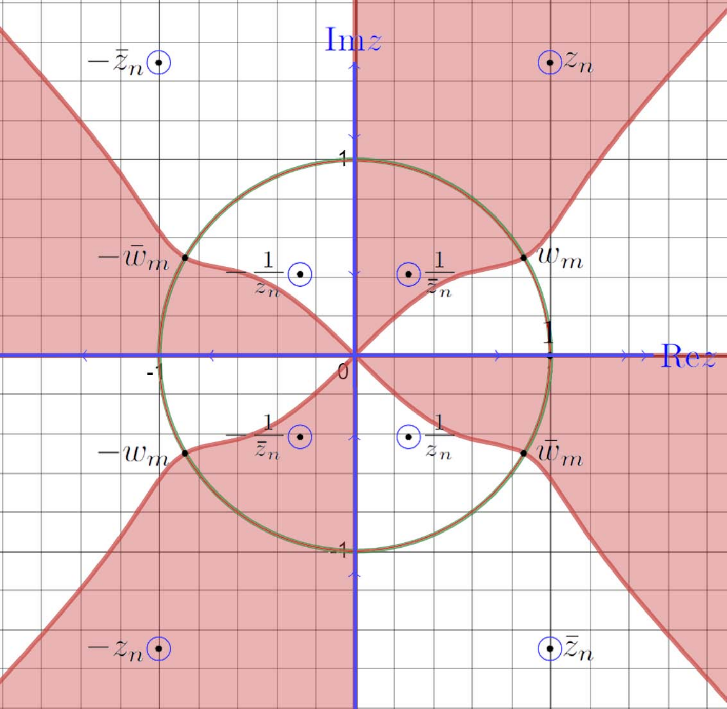
The signature of Im​θ\text{Im}\theta are shown in Figure 3.

Refer to caption
Refer to caption
Refer to caption
Refer to caption
Refer to caption
Refer to caption
Figure 3: In these figure we take ξ=−4,−3,−2.6,−1.5,−1,0\xi=-4,-3,-2.6,-1.5,-1,0 respectively to show all type of Im​θ\text{Im}\theta. The green curve is unit circle. In the red region, Im​θ>0\text{Im}\theta>0 while Im​θ=0\text{Im}\theta=0 on the red curve. And Im​θ<0\text{Im}\theta<0 in the white region.

In our paper, we only consider the case −3<ξ<−1-3<\xi<-1 which is corresponding to Figure 3 (c), because of its well property.

For brevity, we introduce some notations with respect to subscripts

𝒩≜{1,…,4​N1+2​N2},∇={n∈𝒩|Im​θn≤0},\displaystyle\mathcal{N}\triangleq\left\{1,...,4N_{1}+2N_{2}\right\},\ \ \nabla=\left\{n\in\mathcal{N}|\text{Im}\theta_{n}\leq 0\right\},
Δ={n∈𝒩|Im​θn>0},Λ={n∈𝒩|Im​θn=0}.\displaystyle\Delta=\left\{n\in\mathcal{N}|\text{Im}\theta_{n}>0\right\},\Lambda=\left\{n\in\mathcal{N}|\text{Im}\theta_{n}=0\right\}. (3.2)

For n∈Δn\in\Delta, the residue of M⁡(z)M(z) at ζn\zeta_{n} in (2) are unbounded as t→∞t\to\infty. Similarly, for n∈∇n\in\nabla, the residue at ζn\zeta_{n} approach to be zero as t→∞t\to\infty. Define

ρ0=minn∈Δ∪∇∖Λ⁡|Im​θn|≠0.\rho_{0}=\min_{n\in\Delta\cup\nabla\setminus\Lambda}|\text{Im}\theta_{n}|\neq 0. (3.3)

To distinguish different type of zeros, we further give

∇1={j∈{1,…,N1}|Im​θ​(zj)≤0},Δ1={j∈{1,…,N1}|Im​θ​(zj)>0},\displaystyle\nabla_{1}=\left\{j\in\left\{1,...,N_{1}\right\}|\text{Im}\theta(z_{j})\leq 0\right\},\Delta_{1}=\left\{j\in\left\{1,...,N_{1}\right\}|\text{Im}\theta(z_{j})>0\right\},
∇2={i∈{1,…,N2}|Im​θ​(wi)≤0},Δ2={i∈{1,…,N2}|Im​θ​(wi)>0},\displaystyle\nabla_{2}=\left\{i\in\left\{1,...,N_{2}\right\}|\text{Im}\theta(w_{i})\leq 0\right\},\Delta_{2}=\left\{i\in\left\{1,...,N_{2}\right\}|\text{Im}\theta(w_{i})>0\right\},
Λ1={j0∈{1,…,N1}|Imθ(zj0)=0},Λ2={i0∈{1,…,N2}|Imθ(wOPENi0)=0}.\displaystyle\Lambda_{1}=\left\{j_{0}\in\left\{1,...,N_{1}\right\}|\text{Im}\theta(z_{j_{0}})=0\right\},\Lambda_{2}=\left\{i_{0}\in\left\{1,...,N_{2}\right\}|\text{Im}\theta(w_{i_{0})}=0\right\}.

For the poles ζn\zeta_{n} with n∉Λn\notin\Lambda, we want to trap them for jumps along small closed circles enclosing themselves respectively. The jump matrix in (2.41) also needs to be restricted. Recall the well known factorizations of V⁡(z)V(z):

V⁡(z)\displaystyle V(z) =(1−ρ~​e2​i​t​θ01)​(10ρ​e−2​i​t​θ1)\displaystyle=\left(\begin{array}[]{cc}1&-\tilde{\rho}e^{2it\theta}\\ 0&1\end{array}\right)\left(\begin{array}[]{cc}1&0\\ \rho e^{-2it\theta}&1\end{array}\right)
=(1ρ​e−2​i​t​θ1−ρ​ρ~1)​(1−ρ​ρ~)σ3​(1−ρ~​e2​i​t​θ1−ρ​ρ~01).\displaystyle=\left(\begin{array}[]{cc}1&\\ \frac{\rho e^{-2it\theta}}{1-\rho\tilde{\rho}}&1\end{array}\right)(1-\rho\tilde{\rho})^{\sigma_{3}}\left(\begin{array}[]{cc}1&-\frac{\tilde{\rho}e^{2it\theta}}{1-\rho\tilde{\rho}}\\ 0&1\end{array}\right).

We will use these factorizations to deform the jump contours so that exponentials e±2​i​t​θe^{\pm 2it\theta} are decaying in corresponding regions respectively. Define functions

δ⁡(z)\displaystyle\delta(z) =exp(−12​π​i∫i​ℝ(1s−z−12​s)log(1−ρ(s)ρ~(s))ds);\displaystyle=\exp\left(-\frac{1}{2\pi i}\int_{i\mathbb{R}}\left(\dfrac{1}{s-z}-\frac{1}{2s}\right)\log(1-\rho(s)\tilde{\rho}(s))ds\right); (3.12)
T⁡(z)\displaystyle T(z) =T⁡(z,ξ)=∏n∈Δz−ζnζ¯n−1​z−1​δ​(z)\displaystyle=T(z,\xi)=\prod_{n\in\Delta}\dfrac{z-\zeta_{n}}{\bar{\zeta}_{n}^{-1}z-1}\delta(z)
=∏j∈Δ1z2−zj2z¯j−2​z2−1​z2−z¯j−2zj2​z2−1​∏i∈Δ2z2−wi2wi2​z2−1​δ​(z).\displaystyle=\prod_{j\in\Delta_{1}}\dfrac{z^{2}-z_{j}^{2}}{\bar{z}_{j}^{-2}z^{2}-1}\dfrac{z^{2}-\bar{z}_{j}^{-2}}{z_{j}^{2}z^{2}-1}\prod_{i\in\Delta_{2}}\dfrac{z^{2}-w_{i}^{2}}{w_{i}^{2}z^{2}-1}\delta(z). (3.13)

In the above formulas, we choose the principal branch of power and logarithm functions.

Proposition 4.

The function defined by (3.13) has following properties:
(a) TT is meromorphic in ℂ∖ℝ\mathbb{C}\setminus\mathbb{R}, and for each n∈Δn\in\Delta, T⁡(z)T(z) has simple zeros ζn\zeta_{n} and simple poles ζ¯n\bar{\zeta}_{n};
(b) T⁡(z)=T−1​(z¯)¯=T−1​(−z−1)T(z)=\overline{T^{-1}(\bar{z})}=T^{-1}(-z^{-1});
(c) For z∈ℝz\in\mathbb{R}, as z approaching the real axis from above and below, TT has boundary values T±T_{\pm}, which satisfy:

T+​(z)=(1−ρ⁡(z)​ρ~​(z))​T−​(z),z∈i​ℝ;T_{+}(z)=(1-\rho(z)\tilde{\rho}(z))T_{-}(z),\hskip 14.22636ptz\in i\mathbb{R}; (3.14)

(d) limz→∞T⁡(z)≜T⁡(∞)\lim_{z\to\infty}T(z)\triangleq T(\infty), where

T⁡(∞)=∏j∈Δ1z¯j2​zj−2​∏i∈Δ2w¯i2​exp⁡(14​π​i​∫i​ℝs−1​log⁡(1−ρ⁡(s)​ρ~​(s))​𝑑s),T(\infty)=\prod_{j\in\Delta_{1}}\bar{z}_{j}^{2}z_{j}^{-2}\prod_{i\in\Delta_{2}}\bar{w}_{i}^{2}\exp\left(\frac{1}{4\pi i}\int_{i\mathbb{R}}s^{-1}\log(1-\rho(s)\tilde{\rho}(s))ds\right), (3.15)

with |T⁡(∞)|=1|T(\infty)|=1;
(e) As |z|→∞|z|\to\infty with |a​r​g​(z)|≤c<π|arg(z)|\leq c<\pi,

T⁡(z)=T⁡(∞)​(1+z−1​12​π​i​∫i​ℝlog⁡(1−ρ⁡(s)​ρ~​(s))​𝑑s+𝒪⁡(z−2));T(z)=T(\infty)\left(1+z^{-1}\frac{1}{2\pi i}\int_{i\mathbb{R}}\log(1-\rho(s)\tilde{\rho}(s))ds+\mathcal{O}(z^{-2})\right); (3.16)

(f) T⁡(z)T(z) is continuous at z=0z=0, and

limz→0T⁡(z)=T⁡(0)=T​(∞)−1;\lim_{z\to 0}T(z)=T(0)=T(\infty)^{-1}; (3.17)

(g) a⁡(z)T⁡(z)\frac{a(z)}{T(z)} is holomorphic in D+D^{+}. And its absolute value is bounded in D+∩{z∈ℂ|Re​z>0}D^{+}\cap\left\{z\in\mathbb{C}|\text{Re}z>0\right\}. Additionally, the ratio extends as a continuous function on i​ℝi\mathbb{R}.

Proof.

Properties (a), (b), (d) and (f) can be obtain by simple calculation. And (c) follows from the Plemelj formula. By the Laurent expansion (e) immediately. For brevity, we omit calculation. For (g), from (2.37) we have

a⁡(z)T⁡(z)=T(∞)−1∏j∈∇1z2−zj2z¯j−2​z2−1z2−z¯j−2zj2​z2−1∏i∈∇2z2−wi2wi2​z2−1exp{−12​π​i∫ℝlog⁡(1−ρ⁡(s)​ρ~​(s))s−z}.\frac{a(z)}{T(z)}=T(\infty)^{-1}\prod_{j\in\nabla_{1}}\dfrac{z^{2}-z_{j}^{2}}{\bar{z}_{j}^{-2}z^{2}-1}\dfrac{z^{2}-\bar{z}_{j}^{-2}}{z_{j}^{2}z^{2}-1}\prod_{i\in\nabla_{2}}\dfrac{z^{2}-w_{i}^{2}}{w_{i}^{2}z^{2}-1}\exp\left\{-\frac{1}{2\pi i}\int_{\mathbb{R}}\frac{\log(1-\rho(s)\tilde{\rho}(s))}{s-z}\right\}.

So a⁡(z)T⁡(z)\frac{a(z)}{T(z)} is holomorphic in D+D^{+}. And in above expression, all factors except the last integral is bounded for z∈D+z\in D^{+}. From (2.17), 1−ρ⁡(s)​ρ~​(s)=1+|ρ⁡(s)|21-\rho(s)\tilde{\rho}(s)=1+|\rho(s)|^{2}. Let z=x+y​iz=x+yi, then the real part of the exponential is −y2​π∫ℝlog⁡(1+|ρ⁡(s)|2)|s−z|2ds-\frac{y}{2\pi}\int_{\mathbb{R}}\frac{\log(1+|\rho(s)|^{2})}{|s-z|^{2}}ds which can be bounded as follows:

|y2​π​∫ℝlog⁡(1+|ρ⁡(s)|2)|s−z|2​𝑑s|\displaystyle|\frac{y}{2\pi}\int_{\mathbb{R}}\frac{\log(1+|\rho(s)|^{2})}{|s-z|^{2}}ds| ≤12​π∥log(1+|ρ(s)|2)∥L∞​(ℝ)∥y(s−x)2+y2∥L1​(ℝ)\displaystyle\leq\frac{1}{2\pi}\parallel\log(1+|\rho(s)|^{2})\parallel_{L^{\infty}(\mathbb{R})}\parallel\frac{y}{(s-x)^{2}+y^{2}}\parallel_{L^{1}(\mathbb{R})}
≲∥ρ(s)∥L∞​(ℝ).\displaystyle\lesssim\parallel\rho(s)\parallel_{L^{\infty}(\mathbb{R})}.

∎

Additionally, let ϱ\varrho be a positive constant stratifying

ϱ=12​min​{minj≠i∈𝒩⁡|ζi−ζj|,minj∈𝒩⁡{|Im​ζj|,|Re​ζj|},minj∈𝒩∖Λ,Im​θ​(z)=0⁡|ζj−z|}.\varrho=\frac{1}{2}\min\left\{\min_{j\neq i\in\mathcal{N}}|\zeta_{i}-\zeta_{j}|,\min_{j\in\mathcal{N}}\left\{|\text{Im}\zeta_{j}|,|\text{Re}\zeta_{j}|\right\},\min_{j\in\mathcal{N}\setminus\Lambda,\text{Im}\theta(z)=0}|\zeta_{j}-z|\right\}. (3.18)

By above definition, for every n∈𝒩n\in\mathcal{N}, we define disks 𝔻⁡(ζn,ϱ)\mathbb{D}(\zeta_{n},\varrho), such that they pairwise disjoint, also disjoint with {z∈ℂ|Im​θ​(z)=0}\left\{z\in\mathbb{C}|\text{Im}\theta(z)=0\right\} and Σ\Sigma. Introduce a piecewise matrix function

G⁡(z)={(10−Cn​(z−ζn)−1​e−2​i​t​θn1),as z∈𝔻(ζn,ϱ),n∈∇∖Λ;(1−Cn−1​(z−ζn)​e2​i​t​θn01),as z∈𝔻(ζn,ϱ),n∈Δ;(1C¯n​(z−ζ¯n)−1​e2​i​t​θ¯n01),as z∈𝔻(ζ¯n,ϱ),n∈∇∖Λ;(10C¯n−1​(z−ζ¯n)​e−2​i​t​θ¯n1),as z∈𝔻(ζ¯n,ϱ),n∈Δ;Ias ​z​ in elsewhere;.G(z)=\left\{\begin{array}[]{ll}\left(\begin{array}[]{cc}1&0\\ -C_{n}(z-\zeta_{n})^{-1}e^{-2it\theta_{n}}&1\end{array}\right),&\text{as }z\in\mathbb{D}(\zeta_{n},\varrho),n\in\nabla\setminus\Lambda;\\[12.0pt] \left(\begin{array}[]{cc}1&-C_{n}^{-1}(z-\zeta_{n})e^{2it\theta_{n}}\\ 0&1\end{array}\right),&\text{as }z\in\mathbb{D}(\zeta_{n},\varrho),n\in\Delta;\\ \left(\begin{array}[]{cc}1&\bar{C}_{n}(z-\bar{\zeta}_{n})^{-1}e^{2it\bar{\theta}_{n}}\\ 0&1\end{array}\right),&\text{as }z\in\mathbb{D}(\bar{\zeta}_{n},\varrho),n\in\nabla\setminus\Lambda;\\ \left(\begin{array}[]{cc}1&0\\ \bar{C}_{n}^{-1}(z-\bar{\zeta}_{n})e^{-2it\bar{\theta}_{n}}&1\end{array}\right),&\text{as }z\in\mathbb{D}(\bar{\zeta}_{n},\varrho),n\in\Delta;\\ I&\text{as }z\text{ in elsewhere};\end{array}\right.. (3.19)

Now we use T⁡(z)T(z) and G⁡(z)G(z) to define a new matrix-valued function M(1)​(z)M^{(1)}(z).

M(1)​(z)=T​(∞)−σ3​M​(z)​G​(z)​T​(z)σ3,M^{(1)}(z)=T(\infty)^{-\sigma_{3}}M(z)G(z)T(z)^{\sigma_{3}}, (3.20)

which then satisfies the following RH problem.

RHP1. Find a matrix-valued function M(1)​(z)M^{(1)}(z) which satisfies:

▶\blacktriangleright Analyticity: M(1)​(z)M^{(1)}(z) is meromorphic in ℂ∖Σ(1)\mathbb{C}\setminus\Sigma^{(1)}, where

Σ(1)=ℝ∪iℝ∪[∪n∈𝒩∖Λ(∂𝔻(ζ¯n,ϱ)∪∂𝔻(ζn,ϱ))],\Sigma^{(1)}=\mathbb{R}\cup i\mathbb{R}\cup\left[\cup_{n\in\mathcal{N}\setminus\Lambda}\left(\partial\mathbb{D}(\bar{\zeta}_{n},\varrho)\cup\partial\mathbb{D}(\zeta_{n},\varrho)\right)\right], (3.21)

is shown in Figure 4;

▶\blacktriangleright Symmetry: M(1)​(z)=σ2​M(1)​(z¯)¯​σ2M^{(1)}(z)=\sigma_{2}\overline{M^{(1)}(\bar{z})}\sigma_{2}=σ1M(1)​(−z¯)¯σ1=izM(1)(−1/z)σ3Q−\sigma_{1}\overline{M^{(1)}(-\bar{z})}\sigma_{1}=\frac{i}{z}M^{(1)}(-1/z)\sigma_{3}Q_{-};

▶\blacktriangleright Jump condition: M(1)M^{(1)} has continuous boundary values M±(1)M^{(1)}_{\pm} on Σ(1)\Sigma^{(1)} and

M+(1)​(z)=M−(1)​(z)​V(1)​(z),z∈Σ(1),M^{(1)}_{+}(z)=M^{(1)}_{-}(z)V^{(1)}(z),\hskip 14.22636ptz\in\Sigma^{(1)}, (3.22)

where

V(1)​(z)={(1−e2​i​t​θ​ρ~​(z)​T−2​(z)01)​(10e−2​i​t​θ​ρ​(z)​T2​(z)1),as ​z∈ℝ;(10e−2​i​t​θ​ρ~​(z)​T+2​(z)1−ρ~​(z)​ρ​(z)1)​(1−e2​i​t​θ​ρ~​(z)​T−−2​(z)1−ρ~​(z)​ρ​(z)01),as ​z∈i​ℝ;(10−Cn​(z−ζn)−1​T2​(z)​e−2​i​t​θn1),as z∈∂𝔻(ζn,ϱ),n∈∇∖Λ;(1−Cn−1​(z−ζn)​T−2​(z)​e2​i​t​θn01),as z∈∂𝔻(ζn,ϱ),n∈Δ;(1C¯n​(z−ζ¯n)−1​T−2​(z)​e2​i​t​θ¯n01),as z∈∂𝔻(ζ¯n,ϱ),n∈∇∖Λ;(10C¯n−1​(z−ζ¯n)​e−2​i​t​θ¯n​T2​(z)1),as z∈∂𝔻(ζ¯n,ϱ),n∈Δ;;V^{(1)}(z)=\left\{\begin{array}[]{ll}\left(\begin{array}[]{cc}1&-e^{2it\theta}\tilde{\rho}(z)T^{-2}(z)\\ 0&1\end{array}\right)\left(\begin{array}[]{cc}1&0\\ e^{-2it\theta}\rho(z)T^{2}(z)&1\end{array}\right),&\text{as }z\in\mathbb{R};\\[12.0pt] \left(\begin{array}[]{cc}1&0\\ \frac{e^{-2it\theta}\tilde{\rho}(z)T_{+}^{2}(z)}{1-\tilde{\rho}(z)\rho(z)}&1\end{array}\right)\left(\begin{array}[]{cc}1&-\frac{e^{2it\theta}\tilde{\rho}(z)T_{-}^{-2}(z)}{1-\tilde{\rho}(z)\rho(z)}\\ 0&1\end{array}\right),&\text{as }z\in i\mathbb{R};\\[12.0pt] \left(\begin{array}[]{cc}1&0\\ -C_{n}(z-\zeta_{n})^{-1}T^{2}(z)e^{-2it\theta_{n}}&1\end{array}\right),&\text{as }z\in\partial\mathbb{D}(\zeta_{n},\varrho),n\in\nabla\setminus\Lambda;\\[12.0pt] \left(\begin{array}[]{cc}1&-C_{n}^{-1}(z-\zeta_{n})T^{-2}(z)e^{2it\theta_{n}}\\ 0&1\end{array}\right),&\text{as }z\in\partial\mathbb{D}(\zeta_{n},\varrho),n\in\Delta;\\ \left(\begin{array}[]{cc}1&\bar{C}_{n}(z-\bar{\zeta}_{n})^{-1}T^{-2}(z)e^{2it\bar{\theta}_{n}}\\ 0&1\end{array}\right),&\text{as }z\in\partial\mathbb{D}(\bar{\zeta}_{n},\varrho),n\in\nabla\setminus\Lambda;\\ \left(\begin{array}[]{cc}1&0\\ \bar{C}_{n}^{-1}(z-\bar{\zeta}_{n})e^{-2it\bar{\theta}_{n}}T^{2}(z)&1\end{array}\right),&\text{as }z\in\partial\mathbb{D}(\bar{\zeta}_{n},\varrho),n\in\Delta;\\ \end{array}\right.; (3.23)

▶\blacktriangleright Asymptotic behaviors:

M(1)​(z)=ei​ν−​(x,t,q)​σ3+𝒪⁡(z−1),z→∞,\displaystyle M^{(1)}(z)=e^{i\nu_{-}(x,t;q)\sigma_{3}}+\mathcal{O}(z^{-1}),\hskip 14.22636ptz\rightarrow\infty, (3.24)
M(1)​(z)=iz​ei​ν−​(x,t,q)​σ3​σ3​Q−+𝒪⁡(1),z→0;\displaystyle M^{(1)}(z)=\frac{i}{z}e^{i\nu_{-}(x,t;q)\sigma_{3}}\sigma_{3}Q_{-}+\mathcal{O}(1),\hskip 14.22636ptz\rightarrow 0; (3.25)

▶\blacktriangleright Residue conditions: M(1)M^{(1)} has simple poles at each point ζn\zeta_{n} and ζ¯n\bar{\zeta}_{n} for n∈Λn\in\Lambda with:

Resz=ζnM(1)​(z)=limz→ζnM(1)​(z)​(00Cn​e−2​i​t​θn​T2​(ζn)0),\displaystyle\res_{z=\zeta_{n}}M^{(1)}(z)=\lim_{z\to\zeta_{n}}M^{(1)}(z)\left(\begin{array}[]{cc}0&0\\ C_{n}e^{-2it\theta_{n}}T^{2}(\zeta_{n})&0\end{array}\right),
Resz=ζ¯nM(1)​(z)=limz→ζ¯nM(1)​(z)​(0−C¯n​T−2​(ζ¯n)​e2​i​t​θ¯n00).\displaystyle\res_{z=\bar{\zeta}_{n}}M^{(1)}(z)=\lim_{z\to\bar{\zeta}_{n}}M^{(1)}(z)\left(\begin{array}[]{cc}0&-\bar{C}_{n}T^{-2}(\bar{\zeta}_{n})e^{2it\bar{\theta}_{n}}\\ 0&0\end{array}\right).
Proof.

Note that the triangular factors (3.19) trades poles ζn\zeta_{n} and ζ¯n\bar{\zeta}_{n} to jumps on the disk boundaries ∂𝔻⁡(ζn,ϱ)\partial\mathbb{D}(\zeta_{n},\varrho) and ∂𝔻⁡(ζ¯n,ϱ)\partial\mathbb{D}(\bar{\zeta}_{n},\varrho) respectively for n∈𝒩∖Λn\in\mathcal{N}\setminus\Lambda. Then by simple calculation we can obtain the residues condition and jump condition from (2), (2) (2.41), (3.19) and (3.20). The analyticity and symmetry of M(1)​(z)M^{(1)}(z) is directly from its definition, the Proposition 4, (3.19) and the properties of MM. As for asymptotic behaviors, from limz→0G⁡(z)=limz→∞G⁡(z)=I\lim_{z\to 0}G(z)=\lim_{z\to\infty}G(z)=I and Proposition 4 (f), we obtain that M(1)​(z)M^{(1)}(z) has same asymptotic behaviors as M⁡(z)M(z). ∎

Figure 4: The blue curve, including ℝ\mathbb{R}, i​ℝi\mathbb{R} and the small circles constitute Σ(1)\Sigma^{(1)}. Because Imθ⁡(wm)=0\theta(w_{m})=0, it remain the pole of M(1)M^{(1)}. And Imθ⁡(zn)≠0\theta(z_{n})\neq 0, so we change it to jump on ∂𝔻⁡(ζn,ϱ)\partial\mathbb{D}(\zeta_{n},\varrho).
Refer to caption

4 Mixed ∂¯\bar{\partial}-RH Problem

In this section, we make continuous extension for the jump matrix V(1)V^{(1)} to remove the jump from Σ\Sigma. Besides, the new problem is hoped to takes advantage of the decay/growth of e2​i​t​θ​(z)e^{2it\theta(z)} for z∉Σz\notin\Sigma. For this purpose, we introduce new eight regions:

Ω2​n+1={z∈ℂ|n​π/2≤arg⁡z≤n​π/2+φ},\displaystyle\Omega_{2n+1}=\left\{z\in\mathbb{C}|n\pi/2\leq\arg z\leq n\pi/2+\varphi\right\}, (4.1)
Ω2​n+2={z∈ℂ|(n+1)​π/2−φ≤arg⁡z≤(n+1)​π/2},\displaystyle\Omega_{2n+2}=\left\{z\in\mathbb{C}|(n+1)\pi/2-\varphi\leq\arg z\leq(n+1)\pi/2\right\}, (4.2)

where n=0,1,2,3n=0,1,2,3 and φ>0\varphi>0 is an fixed sufficiently small angle achieving following conditions:
1. 2​|ξ+2||ξ+2|+1<cos⁡2​φ<1\frac{2|\xi+2|}{|\xi+2|+1}<\cos 2\varphi<1;
2. each Ωi\Omega_{i} doesn’t intersect any of 𝔻⁡(ζn,ϱ)\mathbb{D}(\zeta_{n},\varrho) or 𝔻⁡(ζ¯n,ϱ)\mathbb{D}(\bar{\zeta}_{n},\varrho).
Define new contours as follow:

Σk=e(k−1)​i​π/4+φR+,k=1,3,5,7,\displaystyle\Sigma_{k}=e^{(k-1)i\pi/4+\varphi}R_{+},\hskip 14.22636ptk=1,3,5,7, (4.3)
Σk=ek​i​π/4−φR+,k=2,4,6,8,\displaystyle\Sigma_{k}=e^{ki\pi/4-\varphi}R_{+},\hskip 14.22636ptk=2,4,6,8, (4.4)
Σ~=Σ1∪Σ2​…∪Σ8,\displaystyle\tilde{\Sigma}=\Sigma_{1}\cup\Sigma_{2}...\cup\Sigma_{8}, (4.5)

which is the boundary of Ωk\Omega_{k} respectively. In addition, let

Ω=Ω1∪…∪Ω8.\displaystyle\Omega=\Omega_{1}\cup...\cup\Omega_{8}. (4.6)
Σ(2)=∪n∈𝒩∖Λ(∂𝔻(ζ¯n,ϱ)∪∂𝔻(ζn,ϱ)),\displaystyle\Sigma^{(2)}=\cup_{n\in\mathcal{N}\setminus\Lambda}\left(\partial\mathbb{D}(\bar{\zeta}_{n},\varrho)\cup\partial\mathbb{D}(\zeta_{n},\varrho)\right), (4.7)

which are shown in Figure 5.

Σ1\Sigma_{1}Σ2\Sigma_{2}Σ3\Sigma_{3}Σ4\Sigma_{4}Σ5\Sigma_{5}Σ6\Sigma_{6}Σ7\Sigma_{7}Σ8\Sigma_{8}RezzImzzΩ3\Omega_{3}Ω2\Omega_{2}Ω1\Omega_{1}Ω6\Omega_{6}Ω5\Omega_{5}Ω4\Omega_{4}Ω7\Omega_{7}Ω8\Omega_{8}00znz_{n}z¯n\bar{z}_{n}−1zn-\frac{1}{z_{n}}−1z¯n-\frac{1}{\bar{z}_{n}}1z¯n\frac{1}{\bar{z}_{n}}1zn\frac{1}{z_{n}}−z¯n-\bar{z}_{n}−zn-z_{n}11wmw_{m}w¯m\bar{w}_{m}−w¯m-\bar{w}_{m}−wm-w_{m}
Figure 5: The yellow region is Ω\Omega. The blue circle constitute Σ(2)\Sigma^{(2)} together.
Lemma 1.

Let ξ=xt∈(−3,−1)\xi=\frac{x}{t}\in(-3,-1), and F⁡(r)=r2+1r2F(r)=r^{2}+\frac{1}{r^{2}} is a real-valued function. Then for z=r​ei​ϕz=re^{i\phi}, the imaginary part of phase function (3.1) satisfies

Im ​θ​(z)≤116|sin⁡2​ϕ|(|ξ+2|−1)​F​(r)2,as ​z∈Ω1,Ω3,Ω5,Ω7;\displaystyle\text{Im }\theta(z)\leq\frac{1}{16}|\sin 2\phi|(|\xi+2|-1)F(r)^{2},\hskip 14.22636pt\text{as }z\in\Omega_{1},\Omega_{3},\Omega_{5},\Omega_{7}; (4.8)
Im ​θ​(z)≥116|sin⁡2​ϕ|(1−|ξ+2|)​F​(r)2,as ​z∈Ω2,Ω4,Ω6,Ω8.\displaystyle\text{Im }\theta(z)\geq\frac{1}{16}|\sin 2\phi|(1-|\xi+2|)F(r)^{2},\hskip 14.22636pt\text{as }z\in\Omega_{2},\Omega_{4},\Omega_{6},\Omega_{8}. (4.9)
Proof.

We only prove the case z∈Ω1,z\in\Omega_{1}, and the other regions are similarly. From (3.1) we have

Im ​θ​(z)\displaystyle\text{Im }\theta(z) =12​Im​z​Re​z​[(ξ+2)​(1+|z|−4)−(Re2​z−Im2​z)​(1+|z|−8)]\displaystyle=\frac{1}{2}\text{Im}z\text{Re}z\left[\left(\xi+2\right)\left(1+|z|^{-4}\right)-\left(\text{Re}^{2}z-\text{Im}^{2}z\right)\left(1+|z|^{-8}\right)\right]
=14​r2​sin⁡2​ϕ​[(ξ+2)​(1+r−4)−r2​cos⁡2​ϕ​(1+r−8)]\displaystyle=\frac{1}{4}r^{2}\sin 2\phi\left[\left(\xi+2\right)\left(1+r^{-4}\right)-r^{2}\cos 2\phi\left(1+r^{-8}\right)\right]
=14​sin⁡2​ϕ​[(ξ+2)​F​(r)−cos⁡2​ϕ​(F​(r)2−2)].\displaystyle=\frac{1}{4}\sin 2\phi\left[\left(\xi+2\right)F(r)-\cos 2\phi\left(F(r)^{2}-2\right)\right]. (4.10)

F⁡(r)≥2F(r)\geq 2 leads to 2≤F​(r)222\leq\frac{F(r)^{2}}{2}. For z∈Ω1z\in\Omega_{1}, 2​|ξ+2||ξ+2|+1<cos⁡2​φ<cos⁡2​ϕ\frac{2|\xi+2|}{|\xi+2|+1}<\cos 2\varphi<\cos 2\phi, then we have

|ξ+2|cos⁡2​ϕ​F​(r)≤|ξ+2|+14​F​(r)2.\frac{|\xi+2|}{\cos 2\phi}F(r)\leq\frac{|\xi+2|+1}{4}F(r)^{2}. (4.11)

Substitute above inequality into (4.10) we obtain the consequence immediately. ∎

Introduce a small enough constant 1>ϵ0>01>\epsilon_{0}>0 with (1−ϵ0)​cos⁡φ>12(1-\epsilon_{0})\cos\varphi>\frac{1}{2}. Let X1∈C0∞​(ℝ,[0,1])X_{1}\in C_{0}^{\infty}\left(\mathbb{R},[0,1]\right), which is support in (1−ϵ0,1+ϵ0)(1-\epsilon_{0},1+\epsilon_{0}). And X0X_{0} has support in (−ϵ0,ϵ0)(-\epsilon_{0},\epsilon_{0}) with X0​(z)=X1​(1+z)X_{0}(z)=X_{1}(1+z). In addition, we denote following functions for brief:

p1​(z)=p5​(z)=ρ⁡(z),p2​(z)=p6​(z)=ρ~​(z)1−ρ⁡(z)​ρ~​(z),\displaystyle p_{1}(z)=p_{5}(z)=\rho(z),\hskip 14.22636ptp_{2}(z)=p_{6}(z)=\dfrac{\tilde{\rho}(z)}{1-\rho(z)\tilde{\rho}(z)}, (4.12)
p3​(z)=p7​(z)=ρ⁡(z)1−ρ⁡(z)​ρ~​(z),p4​(z)=p8​(z)=ρ~​(z).\displaystyle p_{3}(z)=p_{7}(z)=\dfrac{\rho(z)}{1-\rho(z)\tilde{\rho}(z)},\hskip 14.22636ptp_{4}(z)=p_{8}(z)=\tilde{\rho}(z). (4.13)

Then the next step is to construct a matrix function R(2)R^{(2)}. We need to remove jump on ℝ\mathbb{R} and i​ℝi\mathbb{R}, and have some mild control on ∂¯​R(2)\bar{\partial}R^{(2)} sufficient to ensure that the ∂¯\bar{\partial}-contribution to the long-time asymptotics of q⁡(x,t)q(x,t) is negligible. So we choose R(2)​(z)R^{(2)}(z) as

R(2)​(z)={(1Rj​(z)​e2​i​t​θ01),z∈Ωj,j=2,4,6,8;(10Rj​(z)​e−2​i​t​θ1),z∈Ωj,j=1,3,5,7;I,e​l​s​e​w​h​e​r​e;R^{(2)}(z)=\left\{\begin{array}[]{lll}\left(\begin{array}[]{cc}1&R_{j}(z)e^{2it\theta}\\ 0&1\end{array}\right),&z\in\Omega_{j},j=2,4,6,8;\\ \\ \left(\begin{array}[]{cc}1&0\\ R_{j}(z)e^{-2it\theta}&1\end{array}\right),&z\in\Omega_{j},j=1,3,5,7;\\ \\ I,&elsewhere;\\ \end{array}\right. (4.14)

where the functions RjR_{j}, j=1,2,..,8j=1,2,..,8, is defined in following Proposition.

Proposition 5.

RjR_{j}: Ω¯j→C\bar{\Omega}_{j}\to C, j=1,2,..,8j=1,2,..,8 have boundary values as follow:

R1​(z)={−ρ⁡(z)​T​(z)2z∈ℝ+,0z∈Σ1,,R2​(z)={0z∈Σ2,ρ~​(z)​T+​(z)21−ρ⁡(z)​ρ~​(z)z∈i​ℝ+,\displaystyle R_{1}(z)=\Bigg\{\begin{array}[]{ll}-\rho(z)T(z)^{2}&z\in\mathbb{R}^{+},\\ 0&z\in\Sigma_{1},\\ \end{array},\hskip 17.07182ptR_{2}(z)=\Bigg\{\begin{array}[]{ll}0&z\in\Sigma_{2},\\ \dfrac{\tilde{\rho}(z)T_{+}(z)^{2}}{1-\rho(z)\tilde{\rho}(z)}&z\in i\mathbb{R}^{+},\\ \end{array}
R3​(z)={ρ⁡(z)​T−​(z)21−ρ⁡(z)​ρ~​(z)z∈i​ℝ+,0z∈Σ3,,R4​(z)={0z∈Σ4,−ρ~​(z)​T​(z)−2z∈ℝ−,\displaystyle R_{3}(z)=\Bigg\{\begin{array}[]{ll}\dfrac{\rho(z)T_{-}(z)^{2}}{1-\rho(z)\tilde{\rho}(z)}&z\in i\mathbb{R}^{+},\\ 0&z\in\Sigma_{3},\\ \end{array},R_{4}(z)=\Bigg\{\begin{array}[]{ll}0&z\in\Sigma_{4},\\ -\tilde{\rho}(z)T(z)^{-2}&z\in\mathbb{R}^{-},\\ \end{array}
R5​(z)={−ρ⁡(z)​T​(z)2z∈ℝ−,0z∈Σ5,,R6​(z)={0z∈Σ6,ρ~​(z)​T+​(z)21−ρ⁡(z)​ρ~​(z)z∈i​ℝ−,\displaystyle R_{5}(z)=\Bigg\{\begin{array}[]{ll}-\rho(z)T(z)^{2}&z\in\mathbb{R}^{-},\\ 0&z\in\Sigma_{5},\end{array},\hskip 14.22636ptR_{6}(z)=\Bigg\{\begin{array}[]{ll}0&z\in\Sigma_{6},\\ \dfrac{\tilde{\rho}(z)T_{+}(z)^{2}}{1-\rho(z)\tilde{\rho}(z)}&z\in i\mathbb{R}^{-},\\ \end{array}
R7​(z)={ρ⁡(z)​T−​(z)21−ρ⁡(z)​ρ~​(z)z∈i​ℝ−,0z∈Σ7,,R8​(z)={0z∈Σ8,−ρ~​(z)​T​(z)−2z∈ℝ+.\displaystyle R_{7}(z)=\Bigg\{\begin{array}[]{ll}\dfrac{\rho(z)T_{-}(z)^{2}}{1-\rho(z)\tilde{\rho}(z)}&z\in i\mathbb{R}^{-},\\ 0&z\in\Sigma_{7},\end{array},\hskip 17.07182ptR_{8}(z)=\Bigg\{\begin{array}[]{ll}0&z\in\Sigma_{8},\\ -\tilde{\rho}(z)T(z)^{-2}&z\in\mathbb{R}^{+}.\\ \end{array}

RjR_{j} have following property: for j=1,5,4,8,j=1,5,4,8,

|∂¯Rj(z)|≲|pj′(|z|)|+|z|−1/2,for all z∈Ωj;\displaystyle|\bar{\partial}R_{j}(z)|\lesssim|p_{j}^{\prime}(|z|)|+|z|^{-1/2},\text{for all $z\in\Omega_{j}$;} (4.31)

and for j=2,3,6,7,j=2,3,6,7,

|∂¯​Rj​(z)|≲|z∓i|,for all z∈Ωj in a small fixed neighborhood of ±i,\displaystyle|\bar{\partial}R_{j}(z)|\lesssim|z\mp i|,\text{for all $z\in\Omega_{j}$ in a small fixed neighborhood of $\pm i$}, (4.32)
|∂¯Rj(z)|≲|pj′(i|z|)|+|z|−1/2+|∂¯X1(|z|)|,for all z∈Ωj.\displaystyle|\bar{\partial}R_{j}(z)|\lesssim|p_{j}^{\prime}(i|z|)|+|z|^{-1/2}+|\bar{\partial}X_{1}(|z|)|,\text{for all $z\in\Omega_{j}$}. (4.33)

And

∂¯​Rj​(z)=0,if ​z∈e​l​s​e​w​h​e​r​e.\bar{\partial}R_{j}(z)=0,\hskip 14.22636pt\text{if }z\in elsewhere. (4.34)
Proof.

Case I: z∈Ω¯jz\in\bar{\Omega}_{j}, j=1,5,4,8j=1,5,4,8.
Take R1​(z)R_{1}(z) as an example with extensions

R1​(z)=p1​(|z|)​T2​(z)​cos⁡(k0​arg⁡z),k0=2​πφ.R_{1}(z)=p_{1}(|z|)T^{2}(z)\cos(k_{0}\arg z),\hskip 14.22636ptk_{0}=\frac{2\pi}{\varphi}. (4.35)

The other cases are easily inferred. p1​(|z|)=ρ⁡(|z|)p_{1}(|z|)=\rho(|z|) is bounded. Denote z=r​ei​ϕz=re^{i\phi}, then we have ∂¯=ei​ϕ2(∂r+ir∂ϕ)\bar{\partial}=\frac{e^{i\phi}}{2}\left(\partial_{r}+\frac{i}{r}\partial_{\phi}\right). So

∂¯​R1​(z)=ei​ϕ2​T2​(z)​(p1′​(r)​cos⁡(k0​ϕ)−ir​p1​(r)​k0​sin⁡(k0​ϕ)).\displaystyle\bar{\partial}R_{1}(z)=\frac{e^{i\phi}}{2}T^{2}(z)\left(p_{1}^{\prime}(r)\cos(k_{0}\phi)-\frac{i}{r}p_{1}(r)k_{0}\sin(k_{0}\phi)\right). (4.36)

To bound second term we use Cauchy-Schwarz inequality and obtain

|p1(r)|=|ρ(r)|=|ρ(r)−ρ(0)|=|∫0rρ′(s)ds|≤∥ρ′(s)∥L2r1/2.|p_{1}(r)|=|\rho(r)|=|\rho(r)-\rho(0)|=|\int_{0}^{r}\rho^{\prime}(s)ds|\leq\parallel\rho^{\prime}(s)\parallel_{L^{2}}r^{1/2}. (4.37)

And note that T⁡(z)T(z) is a bounded function in Ω¯1\bar{\Omega}_{1}. Then the boundedness of (4.31) follows immediately.
Case II: z∈Ω¯jz\in\bar{\Omega}_{j}, j=2,3,6,7.j=2,3,6,7.
The details of the proof are only given for R2R_{2}. Unlike the vanishing boundary condition case in [16], the determinant of M⁡(z)M(z) is 1+z−21+z^{-2}. So to bound the ∂¯\bar{\partial}-derivative construct by R(2)R^{(2)} in following section, the property of R(2)R^{(2)} at ±i\pm i needs to be control. For this purpose, we make small adjustments to the extensions of R2R_{2} as

R2​(z)=R21​(z)+R22​(z),R_{2}(z)=R_{21}(z)+R_{22}(z), (4.38)

with a constant δ0\delta_{0} stratifying φ>δ0​ϵ0\varphi>\delta_{0}\epsilon_{0} and

R21​(z)\displaystyle R_{21}(z) =[1−X1​(|z|)]​p2​(i​|z|)​T−2​(z)​cos⁡[k0​(π2−arg⁡z)],\displaystyle=[1-X_{1}(|z|)]p_{2}(i|z|)T^{-2}(z)\cos[k_{0}(\frac{\pi}{2}-\arg z)], (4.39)
R22​(z)\displaystyle R_{22}(z) =f⁡(|z|)​g​(z)​cos⁡[k0​(π2−arg⁡z)]\displaystyle=f(|z|)g(z)\cos[k_{0}(\frac{\pi}{2}-\arg z)]
−i​|z|k0​X0​(arg⁡zδ0)​f′​(|z|)​g​(z)​sin⁡[k0​(π2−arg⁡z)].\displaystyle-\frac{i|z|}{k_{0}}X_{0}(\frac{\arg z}{\delta_{0}})f^{\prime}(|z|)g(z)\sin[k_{0}(\frac{\pi}{2}-\arg z)]. (4.40)

Among above function,

f⁡(z)=X1​(z)​b¯​(z)a⁡(z),g⁡(z)=(a⁡(z)T⁡(z))2.\displaystyle f(z)=X_{1}(z)\frac{\bar{b}(z)}{a(z)},\hskip 14.22636ptg(z)=\left(\frac{a(z)}{T(z)}\right)^{2}. (4.41)

Then f⁡(z)∈W​2,∞f(z)\in W{2,\infty}. Obviously, R21​(z)≡0R_{21}(z)\equiv 0 with |z||z| in the support of X1X_{1} and R22​(z)≡0R_{22}(z)\equiv 0 out the support of X1X_{1}. Note that

|p2​(z)|=|ρ~​(z)1−ρ⁡(z)​ρ~​(z)|=|ρ~​(z)1−|ρ⁡(z)|2|≲|ρ⁡(z)|,for z out of supp​(X1).\displaystyle|p_{2}(z)|=|\dfrac{\tilde{\rho}(z)}{1-\rho(z)\tilde{\rho}(z)}|=|\dfrac{\tilde{\rho}(z)}{1-|\rho(z)|^{2}}|\lesssim|\rho(z)|,\hskip 14.22636pt\text{for $z$ out of supp}(X_{1}). (4.42)

Similarly in case I, R21​(z)R_{21}(z) can be bounded as

|∂¯R21(z)|≲(1−X1(|z|))(|p2′(i|z|)|+|z|−1/2)+|∂¯X1(|z|)|.|\bar{\partial}R_{21}(z)|\lesssim(1-X_{1}(|z|))\left(|p_{2}^{\prime}(i|z|)|+|z|^{-1/2}\right)+|\bar{\partial}X_{1}(|z|)|. (4.43)

As for R22​(z)R_{22}(z), z=r​ei​ϕz=re^{i\phi},

∂¯​R22​(z)=\displaystyle\bar{\partial}R_{22}(z)= ei​ϕ2​g​(z)​cos⁡[k0​(π2−φ)]​f′​(i​r)​(1−X0​(φδ0))\displaystyle\frac{e^{i\phi}}{2}g(z)\cos[k_{0}(\frac{\pi}{2}-\varphi)]f^{\prime}(ir)\left(1-X_{0}(\frac{\varphi}{\delta_{0}})\right)
+sin⁡[k0​(π2−φ)]​[i​k0r​f​(i​r)+1δ0​k0​X0′​(φδ0)​f′​(i​r)]\displaystyle+\sin[k_{0}(\frac{\pi}{2}-\varphi)]\left[\frac{ik_{0}}{r}f(ir)+\frac{1}{\delta_{0}k_{0}}X_{0}^{\prime}(\frac{\varphi}{\delta_{0}})f^{\prime}(ir)\right]
−ik0​sin⁡[k0​(π2−φ)]​X0​(arg⁡zδ0)​(r​f′​(i​r))′.\displaystyle-\frac{i}{k_{0}}\sin[k_{0}(\frac{\pi}{2}-\varphi)]X_{0}(\frac{\arg z}{\delta_{0}})(rf^{\prime}(ir))^{\prime}. (4.44)

So |∂¯​R22​(z)||\bar{\partial}R_{22}(z)| is bounded, and we can write |∂¯R22(z)|≲X1(z)|z|−1/2|\bar{\partial}R_{22}(z)|\lesssim X_{1}(z)|z|^{-1/2}. So (4.32) is obtained. In addition, for z∼iz\sim i,

|∂¯​R22​(z)|≲|sin⁡[k0​(π2−φ)]|+|1−X0​(φδ0)|=𝒪⁡(φ),|\bar{\partial}R_{22}(z)|\lesssim|\sin[k_{0}(\frac{\pi}{2}-\varphi)]|+|1-X_{0}(\frac{\varphi}{\delta_{0}})|=\mathcal{O}(\varphi), (4.45)

from which (4.32) follows immediately. ∎

In addition, from Proposition 1, R(2)R^{(2)} achieve the symmetry:

R(2)(z)=σ2R(2)​(z¯)¯σ2=σ1R(2)​(−z¯)¯σ1=σ3Q−R(2)(−1/z)σ3Q−.R^{(2)}(z)=\sigma_{2}\overline{R^{(2)}(\bar{z})}\sigma_{2}=\sigma_{1}\overline{R^{(2)}(-\bar{z})}\sigma_{1}=\sigma_{3}Q_{-}R^{(2)}(-1/z)\sigma_{3}Q_{-}. (4.46)

We now use R(2)R^{(2)} to define the new transformation

M(2)​(z)=M(1)​(z)​R(2)​(z),M^{(2)}(z)=M^{(1)}(z)R^{(2)}(z), (4.47)

which satisfies the following mixed ∂¯\bar{\partial}-RH problem.

RHP2. Find a matrix valued function M(2)​(z,x,t)M^{(2)}(z;x,t) with following properties:

▶\blacktriangleright Analyticity: M(2)​(z,x,t)M^{(2)}(z;x,t) is continuous in ℂ\mathbb{C}, sectionally continuous first partial derivatives in ℂ∖(Σ(2)∪{ζn,ζ¯n}n∈Λ)\mathbb{C}\setminus\left(\Sigma^{(2)}\cup\left\{\zeta_{n},\bar{\zeta}_{n}\right\}_{n\in\Lambda}\right) and meromorphic out Ω¯\bar{\Omega};

▶\blacktriangleright Symmetry: M(2)​(z)=σ2​M(2)​(z¯)¯​σ2M^{(2)}(z)=\sigma_{2}\overline{M^{(2)}(\bar{z})}\sigma_{2}=σ1M(2)​(−z¯)¯σ1=izM(2)(−1/z)σ3Q−\sigma_{1}\overline{M^{(2)}(-\bar{z})}\sigma_{1}=\frac{i}{z}M^{(2)}(-1/z)\sigma_{3}Q_{-};

▶\blacktriangleright Jump condition: M(2)M^{(2)} has continuous boundary values M±(2)M^{(2)}_{\pm} on Σ(2)\Sigma^{(2)} and

M+(2)​(z,x,t)=M−(2)​(z,x,t)​V(2)​(z),z∈Σ(2),M^{(2)}_{+}(z;x,t)=M^{(2)}_{-}(z;x,t)V^{(2)}(z),\hskip 14.22636ptz\in\Sigma^{(2)}, (4.48)

where

V(2)​(z)={(10−Cn​(z−ζn)−1​T2​(z)​e−2​i​t​θn1),as z∈∂𝔻(ζn,ϱ),n∈∇∖Λ;(1−Cn−1​(z−ζn)​T−2​(z)​e2​i​t​θn01),as z∈∂𝔻(ζn,ϱ),n∈Δ;(1C¯n​(z−ζ¯n)−1​T−2​(z)​e2​i​t​θ¯n01),as z∈∂𝔻(ζ¯n,ϱ),n∈∇∖Λ;(10C¯n−1​(z−ζ¯n)​e−2​i​t​θ¯n​T2​(z)1),as z∈∂𝔻(ζ¯n,ϱ),n∈Δ;;V^{(2)}(z)=\left\{\begin{array}[]{ll}\left(\begin{array}[]{cc}1&0\\ -C_{n}(z-\zeta_{n})^{-1}T^{2}(z)e^{-2it\theta_{n}}&1\end{array}\right),&\text{as }z\in\partial\mathbb{D}(\zeta_{n},\varrho),n\in\nabla\setminus\Lambda;\\[12.0pt] \left(\begin{array}[]{cc}1&-C_{n}^{-1}(z-\zeta_{n})T^{-2}(z)e^{2it\theta_{n}}\\ 0&1\end{array}\right),&\text{as }z\in\partial\mathbb{D}(\zeta_{n},\varrho),n\in\Delta;\\ \left(\begin{array}[]{cc}1&\bar{C}_{n}(z-\bar{\zeta}_{n})^{-1}T^{-2}(z)e^{2it\bar{\theta}_{n}}\\ 0&1\end{array}\right),&\text{as }z\in\partial\mathbb{D}(\bar{\zeta}_{n},\varrho),n\in\nabla\setminus\Lambda;\\ \left(\begin{array}[]{cc}1&0\\ \bar{C}_{n}^{-1}(z-\bar{\zeta}_{n})e^{-2it\bar{\theta}_{n}}T^{2}(z)&1\end{array}\right),&\text{as }z\in\partial\mathbb{D}(\bar{\zeta}_{n},\varrho),n\in\Delta;\\ \end{array}\right.; (4.49)

▶\blacktriangleright Asymptotic behaviors:

M(2)​(z)=ei​ν−​(x,t,q)​σ3+𝒪⁡(z−1),z→∞,\displaystyle M^{(2)}(z)=e^{i\nu_{-}(x,t;q)\sigma_{3}}+\mathcal{O}(z^{-1}),\hskip 14.22636ptz\rightarrow\infty, (4.50)
M(2)​(z)=iz​ei​ν−​(x,t,q)​σ3​σ3​Q−+𝒪⁡(1),z→0;\displaystyle M^{(2)}(z)=\frac{i}{z}e^{i\nu_{-}(x,t;q)\sigma_{3}}\sigma_{3}Q_{-}+\mathcal{O}(1),\hskip 14.22636ptz\rightarrow 0; (4.51)

▶\blacktriangleright ∂¯\bar{\partial}-Derivative: For z∈ℂz\in\mathbb{C} we have

∂¯​M(2)=M(2)​∂¯​R(2),\displaystyle\bar{\partial}M^{(2)}=M^{(2)}\bar{\partial}R^{(2)}, (4.52)

where

∂¯​R(2)={(0∂¯​Rj​(z)​e2​i​t​θ00),z∈Ωj,j=1,3,5,7,(00∂¯​Rj​(z)​e−2​i​t​θ0),z∈Ωj,j=2,4,6,8,0e​l​s​e​w​h​e​r​e;\bar{\partial}R^{(2)}=\left\{\begin{array}[]{lll}\left(\begin{array}[]{cc}0&\bar{\partial}R_{j}(z)e^{2it\theta}\\ 0&0\end{array}\right),&z\in\Omega_{j},j=1,3,5,7,\\ \\ \left(\begin{array}[]{cc}0&0\\ \bar{\partial}R_{j}(z)e^{-2it\theta}&0\end{array}\right),&z\in\Omega_{j},j=2,4,6,8,\\ \\ 0&elsewhere;\\ \end{array}\right. (4.53)

▶\blacktriangleright Residue conditions: M(2)M^{(2)} has simple poles at each point ζn\zeta_{n} and ζ¯n\bar{\zeta}_{n} for n∈Λn\in\Lambda with:

Resz=ζnM(2)​(z)=limz→ζnM(2)​(z)​(00Cn​e−2​i​t​θn​T2​(ζn)0),\displaystyle\res_{z=\zeta_{n}}M^{(2)}(z)=\lim_{z\to\zeta_{n}}M^{(2)}(z)\left(\begin{array}[]{cc}0&0\\ C_{n}e^{-2it\theta_{n}}T^{2}(\zeta_{n})&0\end{array}\right),
Resz=ζ¯nM(2)​(z)=limz→ζ¯nM(2)​(z)​(0−C¯n​T−2​(ζ¯n)​e2​i​t​θ¯n00).\displaystyle\res_{z=\bar{\zeta}_{n}}M^{(2)}(z)=\lim_{z\to\bar{\zeta}_{n}}M^{(2)}(z)\left(\begin{array}[]{cc}0&-\bar{C}_{n}T^{-2}(\bar{\zeta}_{n})e^{2it\bar{\theta}_{n}}\\ 0&0\end{array}\right).

5 Decomposition of the mixed ∂¯\bar{\partial}-RH problem

To solve RHP2, we decompose it into a model RH problem for M(r)​(z)M^{(r)}(z) with ∂¯​R(2)≡0\bar{\partial}R^{(2)}\equiv 0 and a pure ∂¯\bar{\partial}-Problem with nonzero ∂¯\bar{\partial}-derivatives. For the first step, we establish a RH problem for the M(r)​(z)M^{(r)}(z) as follows.

RHP3. Find a matrix-valued function M(r)​(z)M^{(r)}(z) with following properties:

▶\blacktriangleright Analyticity: M(r)​(z)M^{(r)}(z) is meromorphic in ℂ∖Σ(2)\mathbb{C}\setminus\Sigma^{(2)};

▶\blacktriangleright Jump condition: MrM^{r} has continuous boundary values M±(r)M^{(r)}_{\pm} on Σ(2)\Sigma^{(2)} and

M+(r)​(z)=M−(r)​(z)​V2​(z),z∈Σ(2);M^{(r)}_{+}(z)=M^{(r)}_{-}(z)V^{2}(z),\hskip 14.22636ptz\in\Sigma^{(2)}; (5.1)

▶\blacktriangleright Symmetry: M(r)​(z)=σ2​M(r)​(z¯)¯​σ2M^{(r)}(z)=\sigma_{2}\overline{M^{(r)}(\bar{z})}\sigma_{2}=σ1M(r)​(−z¯)¯σ1=izM(r)(−1/z)σ3Q−\sigma_{1}\overline{M^{(r)}(-\bar{z})}\sigma_{1}=\frac{i}{z}M^{(r)}(-1/z)\sigma_{3}Q_{-};

▶\blacktriangleright ∂¯\bar{\partial}-Derivative: ∂¯​R(2)=0\bar{\partial}R^{(2)}=0, for z∈ℂz\in\mathbb{C};

▶\blacktriangleright Asymptotic behaviors:

M(r)​(z)=ei​ν−​(x,t,q)​σ3+𝒪⁡(z−1),z→∞,\displaystyle M^{(r)}(z)=e^{i\nu_{-}(x,t;q)\sigma_{3}}+\mathcal{O}(z^{-1}),\hskip 14.22636ptz\rightarrow\infty, (5.2)
M(r)​(z)=iz​ei​ν−​(x,t,q)​σ3​σ3​Q−+𝒪⁡(1),z→0;\displaystyle M^{(r)}(z)=\frac{i}{z}e^{i\nu_{-}(x,t;q)\sigma_{3}}\sigma_{3}Q_{-}+\mathcal{O}(1),\hskip 14.22636ptz\rightarrow 0; (5.3)

▶\blacktriangleright Residue conditions: M(r)M^{(r)} has simple poles at each point ζn\zeta_{n} and ζ¯n\bar{\zeta}_{n} for n∈Λn\in\Lambda with:

Resz=ζnM(r)​(z)=limz→ζnM(r)​(z)​(00Cn​e−2​i​t​θn​T2​(ζn)0),\displaystyle\res_{z=\zeta_{n}}M^{(r)}(z)=\lim_{z\to\zeta_{n}}M^{(r)}(z)\left(\begin{array}[]{cc}0&0\\ C_{n}e^{-2it\theta_{n}}T^{2}(\zeta_{n})&0\end{array}\right),
Resz=ζ¯nM(r)​(z)=limz→ζ¯nM(r)​(z)​(0−C¯n​T−2​(ζ¯n)​e2​i​t​θ¯n00).\displaystyle\res_{z=\bar{\zeta}_{n}}M^{(r)}(z)=\lim_{z\to\bar{\zeta}_{n}}M^{(r)}(z)\left(\begin{array}[]{cc}0&-\bar{C}_{n}T^{-2}(\bar{\zeta}_{n})e^{2it\bar{\theta}_{n}}\\ 0&0\end{array}\right).

The unique existence and asymptotic of M(r)​(z)M^{(r)}(z) will shown in section 6.

We now use M(r)​(z)M^{(r)}(z) to construct a new matrix function

M(3)​(z)=M(2)​(z)​M(r)​(z)−1,M^{(3)}(z)=M^{(2)}(z)M^{(r)}(z)^{-1}, (5.8)

which removes analytical component M(r)​(z)M^{(r)}(z) to get a pure ∂¯\bar{\partial}-problem.

∂¯\bar{\partial}-problem4. Find a matrix-valued function M(3)​(z)M^{(3)}(z) with following properties:

▶\blacktriangleright Analyticity: M(3)​(z)M^{(3)}(z) is continuous and has sectionally continuous first partial derivatives in ℂ\mathbb{C}.

▶\blacktriangleright Asymptotic behavior:

M(3)​(z)∼I+𝒪⁡(z−1),z→∞;\displaystyle M^{(3)}(z)\sim I+\mathcal{O}(z^{-1}),\hskip 14.22636ptz\rightarrow\infty; (5.9)

▶\blacktriangleright ∂¯\bar{\partial}-Derivative: We have

∂¯​M(3)​(z)=M(3)​(z)​W,z∈ℂ,\bar{\partial}M^{(3)}(z)=M^{(3)}(z)W,\ \ z\in\mathbb{C},

where

W=M(r)​(z)​∂¯​R(2)​(z)​M(r)​(z)−1.W=M^{(r)}(z)\bar{\partial}R^{(2)}(z)M^{(r)}(z)^{-1}. (5.10)
Proof.

By using properties of the solutions M(2)​(z)M^{(2)}(z) and M(r)​(z)M^{(r)}(z) for RHP3 and ∂¯\bar{\partial}-problem 4, the analyticity is obtained immediately. And for its Asymptotic behavior, from M(r)​(z)−1=(1+z−2)​σ2​M(r)​(z)T​σ2M^{(r)}(z)^{-1}=(1+z^{-2})\sigma_{2}M^{(r)}(z)^{T}\sigma_{2} we have

limz→0M(3)​(z)=\displaystyle\lim_{z\to 0}M^{(3)}(z)= limz→0(z​M(2)​(z))​σ2​(z​M(r)​(z)T)​σ21+z2\displaystyle\lim_{z\to 0}\dfrac{(zM^{(2)}(z))\sigma_{2}(zM^{(r)}(z)^{T})\sigma_{2}}{1+z^{2}}
=\displaystyle= i​ei​ν−​(x,t,q)​σ3​σ3​Q−​σ2​(i​ei​ν−​(x,t,q)​σ3​σ3​Q−)T​σ2=I.\displaystyle ie^{i\nu_{-}(x,t;q)\sigma_{3}}\sigma_{3}Q_{-}\sigma_{2}(ie^{i\nu_{-}(x,t;q)\sigma_{3}}\sigma_{3}Q_{-})^{T}\sigma_{2}=I. (5.11)

Since M(2)​(z)M^{(2)}(z) and M(r)​(z)M^{(r)}(z) achieve same jump matrix, we have

M−(3)​(z)−1​M+(3)​(z)\displaystyle M_{-}^{(3)}(z)^{-1}M_{+}^{(3)}(z) =M−(2)​(z)−1​M−(r)​(z)​M+(r)​(z)−1​M+(2)​(z)\displaystyle=M_{-}^{(2)}(z)^{-1}M_{-}^{(r)}(z)M_{+}^{(r)}(z)^{-1}M_{+}^{(2)}(z)
=M−(2)​(z)−1​V(2)​(z)−1​M+(2)​(z)=I,\displaystyle=M_{-}^{(2)}(z)^{-1}V^{(2)}(z)^{-1}M_{+}^{(2)}(z)=I,

which implies M(3)​(z)M^{(3)}(z) has no jumps and is everywhere continuous. We also can show that M(3)​(z)M^{(3)}(z) has no pole. For λ∈{ζn,ζ¯n}n∈Λ\lambda\in\left\{\zeta_{n},\bar{\zeta}_{n}\right\}_{n\in\Lambda}, let 𝒩λ\mathcal{N}_{\lambda} denote the nilpotent matrix which appears in the left side of the corresponding residue condition of RHP4 and RHP5, we have the Laurent expansions in z−λz-\lambda

M(2)​(z)=a⁡(λ)​[𝒩λz−λ+I]+𝒪⁡(z−λ),\displaystyle M^{(2)}(z)=a(\lambda)\left[\dfrac{\mathcal{N}_{\lambda}}{z-\lambda}+I\right]+\mathcal{O}(z-\lambda),
M(r)​(z)=A⁡(λ)​[𝒩λz−λ+I]+𝒪⁡(z−λ),\displaystyle M^{(r)}(z)=A(\lambda)\left[\dfrac{\mathcal{N}_{\lambda}}{z-\lambda}+I\right]+\mathcal{O}(z-\lambda),

where a⁡(λ)a(\lambda) and A⁡(λ)A(\lambda) are the constant matrix in their respective expansions. Then

M3​(z)\displaystyle M^{3}(z) ={a⁡(λ)​[𝒩λz−λ+I]}​{[−𝒩λz−λ+I]​σ2​A​(λ)T​σ2}+𝒪⁡(z−λ)\displaystyle=\left\{a(\lambda)\left[\dfrac{\mathcal{N}_{\lambda}}{z-\lambda}+I\right]\right\}\left\{\left[\dfrac{-\mathcal{N}_{\lambda}}{z-\lambda}+I\right]\sigma_{2}A(\lambda)^{T}\sigma_{2}\right\}+\mathcal{O}(z-\lambda)
=𝒪⁡(1),\displaystyle=\mathcal{O}(1), (5.12)

which implies that M(3)​(z)M^{(3)}(z) has removable singularities at λ\lambda. And the ∂¯\bar{\partial}-derivative of M(3)​(z)M^{(3)}(z) come from M(3)​(z)M^{(3)}(z) due to analyticity of M(r)​(z)M^{(r)}(z). In addition, unlike the zero boundary case, we must check its property at ±i\pm i. The symmetries of M(2)​(z)M^{(2)}(z) and M(r)​(z)M^{(r)}(z) imply that

M(2)​(z)=\displaystyle M^{(2)}(z)= (γ±q−​γ±q¯−​γ¯γ¯)+𝒪⁡(z∓i),\displaystyle\left(\begin{array}[]{cc}\gamma&\pm q_{-}\gamma\\ \pm\bar{q}_{-}\bar{\gamma}&\bar{\gamma}\end{array}\right)+\mathcal{O}(z\mp i),
M(r)​(z)=\displaystyle M^{(r)}(z)= ±i2​(z∓i)​(ι¯∓q−​ι∓q¯−​ι¯ι)+𝒪​(1),\displaystyle\dfrac{\pm i}{2(z\mp i)}\left(\begin{array}[]{cc}\bar{\iota}&\mp q_{-}\iota\\ \mp\bar{q}_{-}\bar{\iota}&\iota\end{array}\right)+\mathcal{O}(1),

for two constants γ\gamma and ι\iota. Then the singular part of M(3)​(z)M^{(3)}(z) vanishes at z=±iz=\pm i by simple calculation immediately. ∎

The unique existence and asymptotic of M(3)​(z)M^{(3)}(z) will shown in section 7.

6 Asymptotic of 𝒩⁡(Λ)\mathcal{N}(\Lambda)-soliton solutions

In this section, we build a reflectionless RH problem and show that its solution can approximated with M(r)M^{(r)}.

First we show the existence and uniqueness of solution of the above RHP3 which is related with original RH problem 0.

Proposition 6.

The solution M(r)​(z)M^{(r)}(z) of the RH problem 3 with scattering data {r⁡(z),{ζn,Cn}n∈Λ}\left\{r(z),\left\{\zeta_{n},C_{n}\right\}_{n\in\Lambda}\right\} exists and is unique. By an explicit transformation, M(r)​(z)M^{(r)}(z) is equivalent to a reflectionless solution of the original RHP0 with modified scattering data {0,{ζn,c̊n}n∈Λ}\left\{0,\left\{\zeta_{n},\mathring{c}_{n}\right\}_{n\in\Lambda}\right\}, where

c̊n(x,t)=Cnexp{−1i​π∫ℝlog(1−|ρ(s)|2)(1s−ζn−12​s)}.\mathring{c}_{n}(x,t)=C_{n}\exp\left\{-\frac{1}{i\pi}\int_{\mathbb{R}}\log(1-|\rho(s)|^{2})\left(\frac{1}{s-\zeta_{n}}-\frac{1}{2s}\right)\right\}. (6.1)
Proof.

To transform M(r)​(z)M^{(r)}(z) to the soliton-solution of RHP0, the jumps and poles need to be restored. We reverses the triangularity effected in (3.20) and (4.47):

N⁡(z)=(∏n∈Δζn)−σ3​M(r)​(z)​T−σ^3​G−1​(z)​(∏n∈Δz−ζnζ¯n−1​z−1)−σ3,N(z)=\left(\prod_{n\in\Delta}\zeta_{n}\right)^{-\sigma_{3}}M^{(r)}(z)T^{-\hat{\sigma}_{3}}G^{-1}(z)\left(\prod_{n\in\Delta}\dfrac{z-\zeta_{n}}{\bar{\zeta}_{n}^{-1}z-1}\right)^{-\sigma_{3}}, (6.2)

with G⁡(z)G(z) defined in (3.19). First we verify N⁡(z)N(z) satisfying RHP0. This transformation to N⁡(z)N(z) preserves the normalization conditions at the origin and infinity obviously. And comparing with (3.20), this transformation restore the jump on 𝔻⁡(ζ¯n,ϱ)\mathbb{D}(\bar{\zeta}_{n},\varrho) and 𝔻⁡(ζn,ϱ)\mathbb{D}(\zeta_{n},\varrho) to residue for n∉Λn\notin\Lambda. As for n∈Λn\in\Lambda, take ζn\zeta_{n} as an example. Substitute (5) into the transformation:

Resz=ζnN​(z)=\displaystyle\res_{z=\zeta_{n}}N(z)= (∏n∈Δζn)−σ3​Resz=ζnM(r)​(z)​T−σ^3​G​(z)−1​(∏n∈Δz−ζnζ¯n−1​z−1)−σ3\displaystyle\left(\prod_{n\in\Delta}\zeta_{n}\right)^{-\sigma_{3}}\res_{z=\zeta_{n}}M^{(r)}(z)T^{-\hat{\sigma}_{3}}G(z)^{-1}\left(\prod_{n\in\Delta}\dfrac{z-\zeta_{n}}{\bar{\zeta}_{n}^{-1}z-1}\right)^{-\sigma_{3}}
=\displaystyle= limz→ζn−(∏n∈Δζn)−σ3M(r)(z)(00Cn​e−2​i​t​θn​T2​(ζn)0)(∏n∈Δz−ζnζ¯n−1​z−1)−σ3\displaystyle\lim_{z\to\zeta_{n}}-\left(\prod_{n\in\Delta}\zeta_{n}\right)^{-\sigma_{3}}M^{(r)}(z)\left(\begin{array}[]{cc}0&0\\ C_{n}e^{-2it\theta_{n}}T^{2}(\zeta_{n})&0\end{array}\right)\left(\prod_{n\in\Delta}\dfrac{z-\zeta_{n}}{\bar{\zeta}_{n}^{-1}z-1}\right)^{-\sigma_{3}}
=\displaystyle= limz→ζnN⁡(z)​(00c̊n​e−2​i​t​θn0).\displaystyle\lim_{z\to\zeta_{n}}N(z)\left(\begin{array}[]{cc}0&0\\ \mathring{c}_{n}e^{-2it\theta_{n}}&0\end{array}\right).

Its analyticity and symmetry follow from the Proposition of M(r)​(z)M^{(r)}(z), T⁡(z)T(z) and G⁡(z)G(z) immediately. So N⁡(z)N(z) is solution of RHP0 with absence of reflection, whose unique exact solution exists and can be obtained as described similarly in [18]. So M(r)​(z)M^{(r)}(z) unique exists. ∎

Although M(r)​(z)M^{(r)}(z) admits uniqueness and existence, we can’t give its explicit expression. The jump matrix is uniformly near identity and doesn’t contribute to the asymptotic behavior of the solution.

Lemma 2.

The jump matrix V(2)​(z)V^{(2)}(z) in (4.49) satisfies

∥V(2)−I∥L∞​(Σ(2))=𝒪(e−2​ρ0​t),\displaystyle\parallel V^{(2)}-I\parallel_{L^{\infty}(\Sigma^{(2)})}=\mathcal{\mathcal{O}}(e^{-2\rho_{0}t}), (6.7)

where ρ0\rho_{0} is defined by (3.3).

Proof.

Take z∈∂𝔻⁡(ζn,ϱ),z\in\partial\mathbb{D}(\zeta_{n},\varrho), n∈∇∖Λn\in\nabla\setminus\Lambda as an example.

∥V(2)−I∥L∞​(∂𝔻⁡(ζn,ϱ))\displaystyle\parallel V^{(2)}-I\parallel_{L^{\infty}(\partial\mathbb{D}(\zeta_{n},\varrho))} =|Cn​(z−ζn)−1​T2​(z)​e−2​i​t​θn|\displaystyle=|C_{n}(z-\zeta_{n})^{-1}T^{2}(z)e^{-2it\theta_{n}}|
≲ϱ−1​e−Re​(2​i​t​θn)≲e2​t​Im​(θn)≤e−2​ρ0​t.\displaystyle\lesssim\varrho^{-1}e^{-\text{Re}(2it\theta_{n})}\lesssim e^{2t\text{Im}(\theta_{n})}\leq e^{-2\rho_{0}t}. (6.8)

The last step follows from that for n∈∇∖Λn\in\nabla\setminus\Lambda, Im​θn<0\text{Im}\theta_{n}<0. ∎

Corollary 1.

For 1≤p≤+∞1\leq p\leq+\infty, the jump matrix V(2)​(z)V^{(2)}(z) satisfies

∥V(2)−I∥Lp​(Σ(2))≤Kpe−2​ρ0​t,\parallel V^{(2)}-I\parallel_{L^{p}(\Sigma^{(2)})}\leq K_{p}e^{-2\rho_{0}t}, (6.9)

for some constant Kp≥0K_{p}\geq 0 depending on pp.

This estimation of V(2)V^{(2)} inspires us to consider to completely ignore the jump condition on M(r)​(z)M^{(r)}(z), because there is only exponentially small error (in t). We decompose M(r)​(z)M^{(r)}(z) as

M(r)​(z)=E⁡(z)​MΛ(r)​(z),M^{(r)}(z)=E(z)M^{(r)}_{\Lambda}(z), (6.10)

where E⁡(z)E(z) is a error function, which is a solution of a small-norm RH problem and we discuss it in Section 8. MΛ(r)​(z)M^{(r)}_{\Lambda}(z) solves RHP3 with V(2)≡0V^{(2)}\equiv 0.

RHP5. Find a matrix-valued function MΛ(r)​(z,x,t)M^{(r)}_{\Lambda}(z;x,t) with following properties:

▶\blacktriangleright Analyticity: MΛ(r)​(z,x,t)M^{(r)}_{\Lambda}(z;x,t) is analytical in ℂ∖{ζn,ζ¯n}n∈Λ\mathbb{C}\setminus\left\{\zeta_{n},\bar{\zeta}_{n}\right\}_{n\in\Lambda};

▶\blacktriangleright Symmetry: MΛ(r)​(z)=σ2​MΛ(r)​(z¯)¯​σ2M^{(r)}_{\Lambda}(z)=\sigma_{2}\overline{M^{(r)}_{\Lambda}(\bar{z})}\sigma_{2}=σ1MΛ(r)​(−z¯)¯σ1=izMΛ(r)(−1/z)σ3Q−\sigma_{1}\overline{M^{(r)}_{\Lambda}(-\bar{z})}\sigma_{1}=\frac{i}{z}M^{(r)}_{\Lambda}(-1/z)\sigma_{3}Q_{-};

▶\blacktriangleright Asymptotic behaviors:

MΛ(r)​(z,x,t)=ei​ν−​(x,t,q)​σ3+𝒪⁡(z−1),z→∞,\displaystyle M^{(r)}_{\Lambda}(z;x,t)=e^{i\nu_{-}(x,t;q)\sigma_{3}}+\mathcal{O}(z^{-1}),\hskip 14.22636ptz\rightarrow\infty, (6.11)
MΛ(r)​(z,x,t)=iz​ei​ν−​(x,t,q)​σ3​σ3​Q−+𝒪⁡(1),z→0;\displaystyle M^{(r)}_{\Lambda}(z;x,t)=\frac{i}{z}e^{i\nu_{-}(x,t;q)\sigma_{3}}\sigma_{3}Q_{-}+\mathcal{O}(1),\hskip 14.22636ptz\rightarrow 0; (6.12)

▶\blacktriangleright Residue conditions: MΛ(r)M^{(r)}_{\Lambda} has simple poles at each point ζn\zeta_{n} and ζ¯n\bar{\zeta}_{n} for n∈Λn\in\Lambda with:

Resz=ζnMΛ(r)​(z)=limz→ζnMΛ(r)​(z)​(00Cn​e−2​i​t​θn​T2​(ζn)0),\displaystyle\res_{z=\zeta_{n}}M^{(r)}_{\Lambda}(z)=\lim_{z\to\zeta_{n}}M^{(r)}_{\Lambda}(z)\left(\begin{array}[]{cc}0&0\\ C_{n}e^{-2it\theta_{n}}T^{2}(\zeta_{n})&0\end{array}\right),
Resz=ζ¯nMΛ(r)​(z)=limz→ζ¯nMΛ(r)​(z)​(0−C¯n​T−2​(ζ¯n)​e2​i​t​θ¯n00).\displaystyle\res_{z=\bar{\zeta}_{n}}M^{(r)}_{\Lambda}(z)=\lim_{z\to\bar{\zeta}_{n}}M^{(r)}_{\Lambda}(z)\left(\begin{array}[]{cc}0&-\bar{C}_{n}T^{-2}(\bar{\zeta}_{n})e^{2it\bar{\theta}_{n}}\\ 0&0\end{array}\right).
Proposition 7.

The RHP5 exists an unique solution. Moreover, MΛ(r)​(z)M^{(r)}_{\Lambda}(z) is equivalent to a reflectionless solution of the original RHP0 with modified scattering data {0,{ζn,c̊n}n∈Λ}\left\{0,\left\{\zeta_{n},\mathring{c}_{n}\right\}_{n\in\Lambda}\right\} as follows:
Case I: if Λ=∅\Lambda=\varnothing, then

MΛ(r)​(z)=ei​ν−​(x,t,qΛr)​σ3+iz​ei​ν−​(x,t,qΛr)​σ3​σ3​Q−;M^{(r)}_{\Lambda}(z)=e^{i\nu_{-}(x,t;q^{r}_{\Lambda})\sigma_{3}}+\frac{i}{z}e^{i\nu_{-}(x,t;q^{r}_{\Lambda})\sigma_{3}}\sigma_{3}Q_{-}; (6.17)

Case I: if Λ≠∅\Lambda\neq\varnothing with Λ1={zjk}k=1n1\Lambda_{1}=\left\{z_{j_{k}}\right\}_{k=1}^{n_{1}} and Λ2={wis}s=1n2\Lambda_{2}=\left\{w_{i_{s}}\right\}_{s=1}^{n_{2}}, then

MΛ(r)​(z)\displaystyle M^{(r)}_{\Lambda}(z) =ei​ν−​(x,t,qΛr)​σ3+iz​ei​ν−​(x,t,qΛr)​σ3​σ3​Q−\displaystyle=e^{i\nu_{-}(x,t;q^{r}_{\Lambda})\sigma_{3}}+\frac{i}{z}e^{i\nu_{-}(x,t;q^{r}_{\Lambda})\sigma_{3}}\sigma_{3}Q_{-}
+∑s=1n2[(αsz−wisκs¯z−w¯isκsz−wisαs¯z−w¯is)+(−αsz+wisκs¯z+w¯isκsz+wis−αs¯z+w¯is)]\displaystyle+\sum_{s=1}^{n_{2}}\left[\left(\begin{array}[]{cc}\frac{\alpha_{s}}{z-w_{i_{s}}}&\frac{\overline{\kappa_{s}}}{z-\bar{w}_{i_{s}}}\\ \frac{\kappa_{s}}{z-w_{i_{s}}}&\frac{\overline{\alpha_{s}}}{z-\bar{w}_{i_{s}}}\end{array}\right)+\left(\begin{array}[]{cc}-\frac{\alpha_{s}}{z+w_{i_{s}}}&\frac{\overline{\kappa_{s}}}{z+\bar{w}_{i_{s}}}\\ \frac{\kappa_{s}}{z+w_{i_{s}}}&-\frac{\overline{\alpha_{s}}}{z+\bar{w}_{i_{s}}}\end{array}\right)\right]
+∑k=1n1[(βkz−zjkςk¯z−z¯jkςkz−zjkβk¯z−z¯jk)+(−βkz+zjkςk¯z+z¯jkςkz+zjk−βk¯z+z¯jk)]\displaystyle+\sum_{k=1}^{n_{1}}\left[\left(\begin{array}[]{cc}\frac{\beta_{k}}{z-z_{j_{k}}}&\frac{\overline{\varsigma_{k}}}{z-\bar{z}_{j_{k}}}\\ \frac{\varsigma_{k}}{z-z_{j_{k}}}&\frac{\overline{\beta_{k}}}{z-\bar{z}_{j_{k}}}\end{array}\right)+\left(\begin{array}[]{cc}-\frac{\beta_{k}}{z+z_{j_{k}}}&\frac{\overline{\varsigma_{k}}}{z+\bar{z}_{j_{k}}}\\ \frac{\varsigma_{k}}{z+z_{j_{k}}}&-\frac{\overline{\beta_{k}}}{z+\bar{z}_{j_{k}}}\end{array}\right)\right]
+∑k=1n1i[(−q−​βk¯z¯jk​z−1−q−​ςkzjk​z−1−q−​ςk¯z¯jk​z−1q−​βkzjk​z−1)+(q−​βk¯z¯jk​z+1−q−​ςkzjk​z+1−q−​ςk¯z¯jk​z+1−q−​βkzjk​z+1)],\displaystyle+\sum_{k=1}^{n_{1}}i\left[\left(\begin{array}[]{cc}\frac{-\overline{q_{-}\beta_{k}}}{\bar{z}_{j_{k}}z-1}&\frac{-q_{-}\varsigma_{k}}{z_{j_{k}}z-1}\\ \frac{-\overline{q_{-}\varsigma_{k}}}{\bar{z}_{j_{k}}z-1}&\frac{q_{-}\beta_{k}}{z_{j_{k}}z-1}\end{array}\right)+\left(\begin{array}[]{cc}\frac{\overline{q_{-}\beta_{k}}}{\bar{z}_{j_{k}}z+1}&\frac{-q_{-}\varsigma_{k}}{z_{j_{k}}z+1}\\ \frac{-\overline{q_{-}\varsigma_{k}}}{\bar{z}_{j_{k}}z+1}&\frac{-q_{-}\beta_{k}}{z_{j_{k}}z+1}\end{array}\right)\right],

where βk=βk​(x,t)\beta_{k}=\beta_{k}(x,t), ςk=ςk​(x,t)\varsigma_{k}=\varsigma_{k}(x,t), αs=αs​(x,t)\alpha_{s}=\alpha_{s}(x,t) and κs=κs​(x,t)\kappa_{s}=\kappa_{s}(x,t) with linearly dependant equations:

cjk−1​T​(zjk)−2​e−2​i​θ​(zjk)​t​βk\displaystyle c_{j_{k}}^{-1}T(z_{j_{k}})^{-2}e^{-2i\theta(z_{j_{k}})t}\beta_{k} =izjk​ei​ν−​(x,t,qΛr)​q−+∑h=1n2(κh¯zjk−w¯ih+κh¯zjk+w¯ih)\displaystyle=\frac{i}{z_{j_{k}}}e^{i\nu_{-}(x,t;q^{r}_{\Lambda})}q_{-}+\sum_{h=1}^{n_{2}}\left(\frac{\overline{\kappa_{h}}}{z_{j_{k}}-\bar{w}_{i_{h}}}+\frac{\overline{\kappa_{h}}}{z_{j_{k}}+\bar{w}_{i_{h}}}\right)
+∑l=1n1(ςl¯zjk−z¯jl+ςl¯zjk+z¯jl−i​q−​ςlzjl​zjk−1−i​q−​ςlzjl​zjk+1),\displaystyle+\sum_{l=1}^{n_{1}}\left(\frac{\overline{\varsigma_{l}}}{z_{j_{k}}-\bar{z}_{j_{l}}}+\frac{\overline{\varsigma_{l}}}{z_{j_{k}}+\bar{z}_{j_{l}}}-\frac{iq_{-}\varsigma_{l}}{z_{j_{l}}z_{j_{k}}-1}-\frac{iq_{-}\varsigma_{l}}{z_{j_{l}}z_{j_{k}}+1}\right), (6.30)
cjk−1​T​(zjk)−2​e−2​i​θ​(zjk)​t​ςk\displaystyle c_{j_{k}}^{-1}T(z_{j_{k}})^{-2}e^{-2i\theta(z_{j_{k}})t}\varsigma_{k} =izjk​e−i​ν−​(x,t,qΛr)​q¯−+∑h=1n2(αh¯zjk−w¯ih−αh¯zjk+w¯ih)\displaystyle=\frac{i}{z_{j_{k}}}e^{-i\nu_{-}(x,t;q^{r}_{\Lambda})}\bar{q}_{-}+\sum_{h=1}^{n_{2}}\left(\frac{\overline{\alpha_{h}}}{z_{j_{k}}-\bar{w}_{i_{h}}}-\frac{\overline{\alpha_{h}}}{z_{j_{k}}+\bar{w}_{i_{h}}}\right)
+∑l=1n1(βl¯zjk−z¯jl−βl¯zjk+z¯jl+i​q−​βlzjl​zjk−1−i​q−​βlzjl​zjk+1),\displaystyle+\sum_{l=1}^{n_{1}}\left(\frac{\overline{\beta_{l}}}{z_{j_{k}}-\bar{z}_{j_{l}}}-\frac{\overline{\beta_{l}}}{z_{j_{k}}+\bar{z}_{j_{l}}}+\frac{iq_{-}\beta_{l}}{z_{j_{l}}z_{j_{k}}-1}-\frac{iq_{-}\beta_{l}}{z_{j_{l}}z_{j_{k}}+1}\right), (6.31)

and

cis+N1−1​T​(wis)−2​e−2​i​θ​(wis)​t​αk\displaystyle c_{i_{s}+N_{1}}^{-1}T(w_{i_{s}})^{-2}e^{-2i\theta(w_{i_{s}})t}\alpha_{k} =iwis​ei​ν−​(x,t,qΛr)​q−+∑h=1n2(κh¯wis−w¯ih+κh¯wis+w¯ih)\displaystyle=\frac{i}{w_{i_{s}}}e^{i\nu_{-}(x,t;q^{r}_{\Lambda})}q_{-}+\sum_{h=1}^{n_{2}}\left(\frac{\overline{\kappa_{h}}}{w_{i_{s}}-\bar{w}_{i_{h}}}+\frac{\overline{\kappa_{h}}}{w_{i_{s}}+\bar{w}_{i_{h}}}\right)
+∑l=1n1(ςl¯wis−z¯jl+ςl¯wis+z¯jl−i​q−​ςlzjl​wis−1−i​q−​ςlzjl​wis+1),\displaystyle+\sum_{l=1}^{n_{1}}\left(\frac{\overline{\varsigma_{l}}}{w_{i_{s}}-\bar{z}_{j_{l}}}+\frac{\overline{\varsigma_{l}}}{w_{i_{s}}+\bar{z}_{j_{l}}}-\frac{iq_{-}\varsigma_{l}}{z_{j_{l}}w_{i_{s}}-1}-\frac{iq_{-}\varsigma_{l}}{z_{j_{l}}w_{i_{s}}+1}\right), (6.32)
cis+N1−1​T​(wis)−2​e−2​i​θ​(wis)​t​κk\displaystyle c_{i_{s}+N_{1}}^{-1}T(w_{i_{s}})^{-2}e^{-2i\theta(w_{i_{s}})t}\kappa_{k} =iwis​e−i​ν−​(x,t,qΛr)​q¯−+∑h=1n2(αh¯wis−w¯ih−αh¯wis+w¯ih)\displaystyle=\frac{i}{w_{i_{s}}}e^{-i\nu_{-}(x,t;q^{r}_{\Lambda})}\bar{q}_{-}+\sum_{h=1}^{n_{2}}\left(\frac{\overline{\alpha_{h}}}{w_{i_{s}}-\bar{w}_{i_{h}}}-\frac{\overline{\alpha_{h}}}{w_{i_{s}}+\bar{w}_{i_{h}}}\right)
+∑l=1n1(βl¯wis−z¯jl−βl¯wis+z¯jl+i​q−​βlzjl​wis−1−i​q−​βlzjl​wis+1),\displaystyle+\sum_{l=1}^{n_{1}}\left(\frac{\overline{\beta_{l}}}{w_{i_{s}}-\bar{z}_{j_{l}}}-\frac{\overline{\beta_{l}}}{w_{i_{s}}+\bar{z}_{j_{l}}}+\frac{iq_{-}\beta_{l}}{z_{j_{l}}w_{i_{s}}-1}-\frac{iq_{-}\beta_{l}}{z_{j_{l}}w_{i_{s}}+1}\right), (6.33)

for k=1,…,n1k=1,...,n_{1}, s=1,…,n2s=1,...,n_{2} respectively.

Proof.

The uniqueness of solution follows from the Liouville’s theorem. Case I can be simple obtain. As for Case II, the symmetries of MΛ(r)​(z)M^{(r)}_{\Lambda}(z) means that it admits a partial fraction expansion of following form as above. And to obtain βk\beta_{k}, ςk\varsigma_{k},αs\alpha_{s} and κs\kappa_{s}, we substitute (7) into (6) and obtain four linearly dependant equations set above. ∎

Corollary 2.

When ρ⁡(s)≡0\rho(s)\equiv 0, the scattering matrices S⁡(z)≡IS(z)\equiv I, which means q−=q+q_{-}=q_{+}. Denote qΛr​(x,t)q^{r}_{\Lambda}(x,t) is the 𝒩⁡(Λ)\mathcal{N}(\Lambda)-soliton with scattering data {0,{ζn,c̊n}n∈Λ}\left\{0,\left\{\zeta_{n},\mathring{c}_{n}\right\}_{n\in\Lambda}\right\}. By the reconstruction formula (2.49) and (2.50), the solution qΛr​(x,t)q^{r}_{\Lambda}(x,t) of (1.1) with scattering data {0,{ζn,c̊n}n∈Λ}\left\{0,\left\{\zeta_{n},\mathring{c}_{n}\right\}_{n\in\Lambda}\right\} is given by:

qΛr​(x,t)=ei​ν−​(x,t,qΛr)​limz→∞z​[MΛ(r)]12.\displaystyle q^{r}_{\Lambda}(x,t)=e^{i\nu_{-}(x,t;q^{r}_{\Lambda})}\lim_{z\to\infty}z\left[M^{(r)}_{\Lambda}\right]_{12}. (6.34)

Then in case I,

uΛr​(x,t)=limz→∞z​|[MΛr]12|=1.u^{r}_{\Lambda}(x,t)=\lim_{z\to\infty}z|\left[M^{r}_{\Lambda}\right]_{12}|=1. (6.35)

So ν−​(x,t,qΛr)=0\nu_{-}(x,t;q^{r}_{\Lambda})=0 and

qΛr​(x,t)=q−.\displaystyle q^{r}_{\Lambda}(x,t)=q_{-}. (6.36)

And in case II,

uΛr​(x,t)\displaystyle u^{r}_{\Lambda}(x,t) =limz→∞z​|[MΛ(r)]12|\displaystyle=\lim_{z\to\infty}z|\left[M^{(r)}_{\Lambda}\right]_{12}|
=|i​ei​ν−​(x,t,qΛr)​q−+2​∑s=1n2κ¯k+2​∑k=1n1(ς¯k−i​q−​ςk)|,\displaystyle=|ie^{i\nu_{-}(x,t;q^{r}_{\Lambda})}q_{-}+2\sum_{s=1}^{n_{2}}\bar{\kappa}_{k}+2\sum_{k=1}^{n_{1}}(\bar{\varsigma}_{k}-iq_{-}\varsigma_{k})|, (6.37)

which leads to ν−​(x,t,qΛr)=12​∫−∞x(|uΛr​(y,t)|2−1)​𝑑y\nu_{-}(x,t;q^{r}_{\Lambda})=\frac{1}{2}\int_{-\infty}^{x}(|u^{r}_{\Lambda}(y,t)|^{2}-1)dy and

qΛr​(x,t)\displaystyle q^{r}_{\Lambda}(x,t) =limz→∞ei​ν−​(x,t,qΛr)​z​[MΛ(r)]12\displaystyle=\lim_{z\to\infty}e^{i\nu_{-}(x,t;q^{r}_{\Lambda})}z\left[M^{(r)}_{\Lambda}\right]_{12}
=e2​i​ν−​(x,t,qΛr)​(i​ei​ν−​(x,t,qΛr)​q−+2​∑s=1n2κ¯k+2​∑k=1n1(ς¯k−i​q−​ςk)).\displaystyle=e^{2i\nu_{-}(x,t;q^{r}_{\Lambda})}\left(ie^{i\nu_{-}(x,t;q^{r}_{\Lambda})}q_{-}+2\sum_{s=1}^{n_{2}}\bar{\kappa}_{k}+2\sum_{k=1}^{n_{1}}(\bar{\varsigma}_{k}-iq_{-}\varsigma_{k})\right). (6.38)

7 The small norm RH problem for error function

In this section, we consider the error matrix-function E⁡(z)E(z) and show that for large times, the error function E⁡(z)E(z) solves a small norm RH problem which can be expanded asymptotically. From the definition (6.10), we can obtain a RH problem for the matrix function E⁡(z)E(z).

RHP6 Find a matrix-valued function E⁡(z)E(z) with following properties:

▶\blacktriangleright Analyticity: E⁡(z)E(z) is analytical in ℂ∖Σ(2)\mathbb{C}\setminus\Sigma^{(2)};

▶\blacktriangleright Asymptotic behaviors:

E⁡(z)∼I+𝒪⁡(z−1),|z|→∞;\displaystyle E(z)\sim I+\mathcal{O}(z^{-1}),\hskip 14.22636pt|z|\rightarrow\infty; (7.1)

▶\blacktriangleright Jump condition: EE has continuous boundary values E±E_{\pm} on Σ(2)\Sigma^{(2)} satisfying

E+​(z)=E−​(z)​VE,E_{+}(z)=E_{-}(z)V^{E},

where the jump matrix VEV^{E} is given by

VE​(z)=MΛ(r)​(z)​V(2)​(z)​MΛ(r)​(z)−1.V^{E}(z)=M^{(r)}_{\Lambda}(z)V^{(2)}(z)M^{(r)}_{\Lambda}(z)^{-1}. (7.2)

Proposition 7 implies that MΛ(r)​(z)M^{(r)}_{\Lambda}(z) is bound on Σ(2)\Sigma^{(2)}. By using Lemma 2 and Corollary 1, we have the following estimates

∥VE−I∥Lp≲∥V(2)−I∥Lp=𝒪(e−2​ρ0​t),\parallel V^{E}-I\parallel_{L^{p}}\lesssim\parallel V^{(2)}-I\parallel_{L^{p}}=\mathcal{O}(e^{-2\rho_{0}t}), (7.3)

for 1≤p≤+∞1\leq p\leq+\infty. This uniformly vanishing bound ∥VE−I∥\parallel V^{E}-I\parallel establishes RHP6 as a small-norm RH problem. Therefore, the existence and uniqueness of the RHP6 can shown by using a small-norm RH problem

E⁡(z)=I+12​π​i​∫Σ(2)(I+η⁡(s))​(VE−I)s−z​𝑑s,E(z)=I+\frac{1}{2\pi i}\int_{\Sigma^{(2)}}\dfrac{\left(I+\eta(s)\right)(V^{E}-I)}{s-z}ds, (7.4)

where the η∈L2​(Σ(2))\eta\in L^{2}(\Sigma^{(2)}) is the unique solution of following equation

(1−CE)​η=CE​(I),(1-C_{E})\eta=C_{E}\left(I\right), (7.5)

here CEC_{E}:L2​(Σ(2))→L2​(Σ(2))L^{2}(\Sigma^{(2)})\to L^{2}(\Sigma^{(2)}) is a integral operator defined by

CE​(f)​(z)=C−​(f⁡(VE−I)).C_{E}(f)(z)=C_{-}\left(f(V^{E}-I)\right). (7.6)

The Cauchy projection operator C−C_{-} on Σ(2)\Sigma^{(2)} is

C−​(f)​(s)=limz→Σ−(2)12​π​i​∫Σ(2)f⁡(s)s−z​𝑑s.C_{-}(f)(s)=\lim_{z\to\Sigma^{(2)}_{-}}\frac{1}{2\pi i}\int_{\Sigma^{(2)}}\dfrac{f(s)}{s-z}ds. (7.7)

Then by (7.2) we have

∥CE∥≤∥C−∥∥VE−I∥L∞≲𝒪(e−2​ρ0​t),\parallel C_{E}\parallel\leq\parallel C_{-}\parallel\parallel V^{E}-I\parallel_{L^{\infty}}\lesssim\mathcal{O}(e^{-2\rho_{0}t}), (7.8)

which means ∥CE∥<1\parallel C_{E}\parallel<1 for sufficiently large t, therefore 1−CE1-C_{E} is invertible, and η\eta exists and is unique. Moreover,

∥η∥L2​(Σ(2))≲∥CE∥1−∥CE∥≲𝒪(e−2​ρ0​t).\parallel\eta\parallel_{L^{2}(\Sigma^{(2)})}\lesssim\dfrac{\parallel C_{E}\parallel}{1-\parallel C_{E}\parallel}\lesssim\mathcal{O}(e^{-2\rho_{0}t}). (7.9)

Then we have the existence and boundedness of E⁡(z)E(z). In order to reconstruct the solution q⁡(x,t)q(x,t) of (1.1), we need the asymptotic behavior of E⁡(z)E(z) as z→∞z\to\infty.

Proposition 8.

For E⁡(z)E(z) defined in (7.4), it stratifies

|E⁡(z)−I|≲𝒪⁡(e−2​ρ0​t).|E(z)-I|\lesssim\mathcal{O}(e^{-2\rho_{0}t}). (7.10)

As z→∞z\to\infty, the large zz expansion of EE is

E⁡(z)=I+E1​z−1+𝒪⁡(z−2),\displaystyle E(z)=I+E_{1}z^{-1}+\mathcal{O}(z^{-2}), (7.11)

where

E1=−12​π​i∫Σ(2)(I+η(s))(VE−I)ds,E_{1}=-\frac{1}{2\pi i}\int_{\Sigma^{(2)}}\left(I+\eta(s)\right)(V^{E}-I)ds, (7.12)

satisfying long time asymptotic behavior condition

E1≲𝒪⁡(e−2​ρ0​t).E_{1}\lesssim\mathcal{O}(e^{-2\rho_{0}t}). (7.13)
Proof.

By combining (7.9) and (7.3), we obtain

|E⁡(z)−I|≤|(1−CE)​(η)|+|CE​(η)|≲𝒪⁡(e−2​ρ0​t).|E(z)-I|\leq|(1-C_{E})(\eta)|+|C_{E}(\eta)|\lesssim\mathcal{O}(e^{-2\rho_{0}t}). (7.14)

As z→∞z\to\infty,geometrically expanding (s−z)−1(s-z)^{-1} for zz large in (7.4) leads to (7.11). Finally for E1E_{1},

|E1|≲∥VE−I∥L1+∥η∥L22∥VE−I∥L2≲𝒪(e−2​ρ0​t).\displaystyle|E_{1}|\lesssim\parallel V^{E}-I\parallel_{L^{1}}+\parallel\eta\parallel_{L^{2}}2\parallel V^{E}-I\parallel_{L^{2}}\lesssim\mathcal{O}(e^{-2\rho_{0}t}). (7.15)

∎

8 Analysis on the pure ∂¯\bar{\partial}-Problem

Now we consider the asymptotics behavior of M(3)​(z)M^{(3)}(z). The ∂¯\bar{\partial}-problem 4 of M(3)​(z)M^{(3)}(z) is equivalent to the integral equation

M(3)​(z)=I+1π​∫ℂM(3)​(s)​W(3)​(s)z−s​𝑑m​(s),M^{(3)}(z)=I+\frac{1}{\pi}\int_{\mathbb{C}}\dfrac{M^{(3)}(s)W^{(3)}(s)}{z-s}dm(s), (8.1)

where m⁡(s)m(s) is the Lebesgue measure on the ℂ\mathbb{C}. Denote CzC_{z} as the left Cauchy-Green integral operator defined by

f​Cz​(z)=1π​∫Cf⁡(s)​W(3)​(s)z−s​𝑑m​(s).fC_{z}(z)=\frac{1}{\pi}\int_{C}\dfrac{f(s)W^{(3)}(s)}{z-s}dm(s).

Then above equation (8.1) can be rewritten as

M(3)​(z)=I⋅(I−Cz)−1.M^{(3)}(z)=I\cdot\left(I-C_{z}\right)^{-1}. (8.2)

The existence of operator (I−Cz)−1\left(I-C_{z}\right)^{-1} is given by the following Lemma.

Lemma 3.

The norm of the integral operator CzC_{z} decay to zero as t→∞t\to\infty:

∥Cz∥L∞→L∞≲t−1/2,\parallel C_{z}\parallel_{L^{\infty}\to L^{\infty}}\lesssim t^{-1/2}, (8.3)

which implies that (I−Cz)−1\left(I-C_{z}\right)^{-1} exists.

Proof.

For any f∈L∞f\in L^{\infty},

∥fCz∥L∞\displaystyle\parallel fC_{z}\parallel_{L^{\infty}} ≤∥f∥L∞1π∫C|W(3)​(s)||z−s|dm(s),\displaystyle\leq\parallel f\parallel_{L^{\infty}}\frac{1}{\pi}\int_{C}\dfrac{|W^{(3)}(s)|}{|z-s|}dm(s),

where W⁡(s)=M(r)​(z)​∂¯​R(2)​(z)​M(r)​(z)−1W(s)=M^{(r)}(z)\bar{\partial}R^{(2)}(z)M^{(r)}(z)^{-1}. So we only need to estimate the integral

1π​∫C|W⁡(s)||z−s|​𝑑m​(s).\frac{1}{\pi}\int_{C}\dfrac{|W(s)|}{|z-s|}dm(s).

Since W⁡(s)≡0W(s)\equiv 0 out of Ω¯\bar{\Omega}, we only need to focus on the estimate

1π​∫Ω|W⁡(s)||z−s|​𝑑m​(s).\frac{1}{\pi}\int_{\Omega}\dfrac{|W(s)|}{|z-s|}dm(s).

Unlike the zero boundary case in [16], here detM(r)​(z)=1+z−2\det M^{(r)}(z)=1+z^{-2}, and Proposition 8 implies that |M(r)​(z)|≲1+|z|−2|M^{(r)}(z)|\lesssim\sqrt{1+|z|^{-2}}. So

1π​∫Ω|W⁡(s)||z−s|​𝑑m​(s)≲1π​∫Ω|∂¯​R(2)​(s)||z−s|​1+|s|−2|1+s−2|​𝑑m​(s).\frac{1}{\pi}\int_{\Omega}\dfrac{|W(s)|}{|z-s|}dm(s)\lesssim\frac{1}{\pi}\int_{\Omega}\dfrac{|\bar{\partial}R^{(2)}(s)|}{|z-s|}\frac{1+|s|^{-2}}{|1+s^{-2}|}dm(s). (8.4)

Then for j=1,4,5,8j=1,4,5,8, |M(r)​(z)||M^{(r)}(z)| is bounded in Ωj\Omega_{j}. But when z∈Ωjz\in\Omega_{j} for j=2,3,6,7j=2,3,6,7, the singularity at z=±iz=\pm i need to be treat more carefully. So in following calculation, we take Ω2\Omega_{2} in the second case as an example, because it is more elaborate than Ωj\Omega_{j} for j=1,4,5,8j=1,4,5,8. Denote three sub-region of Ω2\Omega_{2} as

D1=𝔻⁡(0,1−ϵ0)∩Ω2\displaystyle D_{1}=\mathbb{D}(0,1-\epsilon_{0})\cap\Omega_{2} ,D2=𝔻(0,1+ϵ0)∖𝔻(0,1−ϵ0)∩Ω2,\displaystyle,\hskip 8.5359ptD_{2}=\mathbb{D}(0,1+\epsilon_{0})\setminus\mathbb{D}(0,1-\epsilon_{0})\cap\Omega_{2},
D3=Ω2∖𝔻⁡(0,1+ϵ0).\displaystyle D_{3}=\Omega_{2}\setminus\mathbb{D}(0,1+\epsilon_{0}). (8.5)

Then the integral ∫Ω2|W⁡(s)||z−s|​𝑑m​(s)\int_{\Omega_{2}}\dfrac{|W(s)|}{|z-s|}dm(s) is divide to three part:

Ii=∫Di|∂¯​R(2)​(s)||z−s|1+|s|−2|1+s−2|dm(s), for i=1,2,3.\displaystyle I_{i}=\int_{D_{i}}\dfrac{|\bar{\partial}R^{(2)}(s)|}{|z-s|}\frac{1+|s|^{-2}}{|1+s^{-2}|}dm(s),\text{ for }i=1,2,3. (8.6)

Let s=u+v​i=r​ei​ϑs=u+vi=re^{i\vartheta}, z=x+y​iz=x+yi. In the following calculation, we will use the inequality

∥|s−z|−1∥Lq​(ℝ+)={∫0+∞[(v−yu−x)2+1]−q2d(v−y|u−x|)}1q|u−x|−1p≲|u−x|−1p,\parallel|s-z|^{-1}\parallel_{L^{q}(\mathbb{R}^{+})}=\left\{\int^{+\infty}_{0}\left[\left(\frac{v-y}{u-x}\right)^{2}+1\right]^{-\frac{q}{2}}d\left(\frac{v-y}{|u-x|}\right)\right\}^{\frac{1}{q}}|u-x|^{-\frac{1}{p}}\lesssim|u-x|^{-\frac{1}{p}}, (8.7)

with 1≤q<+∞1\leq q<+\infty and 1p+1q=1\frac{1}{p}+\frac{1}{q}=1. For s∈D3s\in D_{3}, |s|>1+ϵ0|s|>1+\epsilon_{0}, then

1+|s|−2|1+s−2|<1+|s|2|s|2−1<1+2ϵ02+2​ϵ0<∞.\frac{1+|s|^{-2}}{|1+s^{-2}|}<\frac{1+|s|^{2}}{|s|^{2}-1}<1+\frac{2}{\epsilon_{0}^{2}+2\epsilon_{0}}<\infty. (8.8)

Then together with (4.14), we have

I3≲∫Ω2|∂¯​R(2)​(s)||z−s|​𝑑m​(s)=∫Ω2|∂¯​R2​(s)​e2​i​t​θ||z−s|​𝑑m​(s).\displaystyle I_{3}\lesssim\int_{\Omega_{2}}\dfrac{|\bar{\partial}R^{(2)}(s)|}{|z-s|}dm(s)=\int_{\Omega_{2}}\dfrac{|\bar{\partial}R_{2}(s)e^{2it\theta}|}{|z-s|}dm(s). (8.9)

Moreover, by Lemma 1,

|e2​i​t​θ|≤e−c​sin⁡2​ϑ​F​(r)2≤e−2​c​u​v≤e−2​c​u,|e^{2it\theta}|\leq e^{-c\sin 2\vartheta F(r)^{2}}\leq e^{-2cuv}\leq e^{-2cu}, (8.10)

where cc is a positive constant, and the last step follows form

v≥max⁡{1+ϵ0,utan⁡φ}≥1+ϵ0>1.v\geq\max\left\{1+\epsilon_{0},\frac{u}{\tan\varphi}\right\}\geq 1+\epsilon_{0}>1.

Substitute (4.31) and above inequality into (8.9) and obtain:

I3≲∫0+∞∫utan⁡φ+∞|p2′​(i​r)|​e−4​c​u​t|z−s|​𝑑v​𝑑u+∫0+∞∫utan⁡φ+∞|r|−1/2e−2​c​u​t|z−s|​𝑑v​𝑑u\displaystyle I_{3}\lesssim\int_{0}^{+\infty}\int_{\frac{u}{\tan\varphi}}^{+\infty}\dfrac{|p_{2}^{\prime}(ir)|e^{-4cut}}{|z-s|}dvdu+\int_{0}^{+\infty}\int_{\frac{u}{\tan\varphi}}^{+\infty}\dfrac{|r|^{-1/2}e^{-2cut}}{|z-s|}dvdu
+∫0+∞∫utan⁡φ+∞|∂¯​X1​(r)|​e−4​c​u​t|z−s|dvdu.\displaystyle+\int_{0}^{+\infty}\int_{\frac{u}{\tan\varphi}}^{+\infty}\dfrac{|\bar{\partial}X_{1}(r)|e^{-4cut}}{|z-s|}dvdu.

By Cauchy-Schwarz inequality, the first item have

∫0+∞∫utan⁡φ+∞|p2′​(i​r)|​e−4​c​u​t|z−s|​𝑑v​𝑑u\displaystyle\int_{0}^{+\infty}\int_{\frac{u}{\tan\varphi}}^{+\infty}\dfrac{|p_{2}^{\prime}(ir)|e^{-4cut}}{|z-s|}dvdu ≤∫0+∞∥ρ~′∥L2​(i​ℝ)∥|s−z|−1∥L2​(ℝ+)e−2​c​u​tdu\displaystyle\leq\int_{0}^{+\infty}\parallel\tilde{\rho}^{\prime}\parallel_{L^{2}(i\mathbb{R})}\parallel|s-z|^{-1}\parallel_{L^{2}(\mathbb{R}^{+})}e^{-2cut}du
≤∫0+∞e−2​c​u​t​|u−x|−12​𝑑u≲t−12.\displaystyle\leq\int_{0}^{+\infty}e^{-2cut}|u-x|^{-\frac{1}{2}}du\lesssim t^{-\frac{1}{2}}. (8.11)

So does the last item. Before we estimating the second item, we consider for p>2p>2,

(∫utan⁡φ+∞|u2+V(2)|−p2​𝑑v)1p\displaystyle\left(\int_{\frac{u}{\tan\varphi}}^{+\infty}|\sqrt{u^{2}+V^{(2)}}|^{-\frac{p}{2}}dv\right)^{\frac{1}{p}} =(∫usin⁡φ+∞|r|−p2+1​v−1​𝑑r)1p≲u−12+1p.\displaystyle=\left(\int_{\frac{u}{\sin\varphi}}^{+\infty}|r|^{-\frac{p}{2}+1}v^{-1}dr\right)^{\frac{1}{p}}\lesssim u^{-\frac{1}{2}+\frac{1}{p}}. (8.12)

Then

∫0+∞∫utan⁡φ+∞|r|−1/2e−2​c​u​t|z−s|​𝑑v​𝑑u\displaystyle\int_{0}^{+\infty}\int_{\frac{u}{\tan\varphi}}^{+\infty}\dfrac{|r|^{-1/2}e^{-2cut}}{|z-s|}dvdu ≤∫0+∞∥|r|∥Lvp​(utan⁡φ,+∞)∥|s−z|−1∥Lq​(ℝ+)e−2​c​u​tdu\displaystyle\leq\int_{0}^{+\infty}\parallel|r|\parallel_{L_{v}^{p}(\frac{u}{\tan\varphi},+\infty)}\parallel|s-z|^{-1}\parallel_{L^{q}(\mathbb{R}^{+})}e^{-2cut}du
≤∫0+∞e−2​c​u​t​|u−x|−1p​u−12+1p​𝑑u≲t−12.\displaystyle\leq\int_{0}^{+\infty}e^{-2cut}|u-x|^{-\frac{1}{p}}u^{-\frac{1}{2}+\frac{1}{p}}du\lesssim t^{-\frac{1}{2}}. (8.13)

Combing above inequality we final have I3≲t−12I_{3}\lesssim t^{-\frac{1}{2}}. As for I2I_{2}, the singularity at ii can be balanced by (4.32), and recall that 1>ϵ0>01>\epsilon_{0}>0 with (1−ϵ0)​cos⁡φ>12(1-\epsilon_{0})\cos\varphi>\frac{1}{2}

I2\displaystyle I_{2} ≲∫02∫1/22e−2​c​u​t|z−s|​1+|s|2|s+i|​𝑑v​𝑑u≲∫02∫1/22e−2​c​u​t|z−s|​𝑑v​𝑑u\displaystyle\lesssim\int_{0}^{2}\int_{1/2}^{2}\dfrac{e^{-2cut}}{|z-s|}\frac{1+|s|^{2}}{|s+i|}dvdu\lesssim\int_{0}^{2}\int_{1/2}^{2}\dfrac{e^{-2cut}}{|z-s|}dvdu
≲∫02|u−x|−1/2e−2​c​u​tdu≲|t|−1/2.\displaystyle\lesssim\int_{0}^{2}|u-x|^{-1/2}e^{-2cut}du\lesssim|t|^{-1/2}. (8.14)

Finally, consider I1I_{1}, similarly we have

I1≲∫01−ϵ0∫u1−ϵ0(|p2′(ir)|+|r|−1/2+|∂¯X1(r)|)e−2​c​u​t|z−s|dvdu,\displaystyle I_{1}\lesssim\int_{0}^{1-\epsilon_{0}}\int_{u}^{1-\epsilon_{0}}\left(|p_{2}^{\prime}(ir)|+|r|^{-1/2}+|\bar{\partial}X_{1}(r)|\right)\dfrac{e^{-2cut}}{|z-s|}dvdu, (8.15)

which can be estimated same as I3I_{3}. So the proof is completed. ∎

As z→∞z\to\infty, M(3)​(z)M^{(3)}(z) has asymptotic expansion:

M(3)​(z)=I−M1(3)​(x,t)​z+𝒪⁡(z−2),M^{(3)}(z)=I-M^{(3)}_{1}(x,t)z+\mathcal{O}(z^{-2}), (8.16)

where M1(3)M^{(3)}_{1} is a zz-independent coefficient. The asymptotic behavior of M1(3)M^{(3)}_{1} given by following Proposition.

Proposition 9.

As z→∞z\to\infty, the expansion above holds with

M1(3)​(x,t)=1π​∫CM(3)​(s)​W(3)​(s)​𝑑m​(s).M^{(3)}_{1}(x,t)=\frac{1}{\pi}\int_{C}M^{(3)}(s)W^{(3)}(s)dm(s). (8.17)

There exist constants T1T_{1}, such that for all t>T1t>T_{1}, M1(3)​(x,t)M^{(3)}_{1}(x,t) satisfies

|M1(3)(x,t)|≲t−3/4.|M^{(3)}_{1}(x,t)|\lesssim t^{-3/4}. (8.18)
Proof.

Lemma 3 and (8.2) implies that for large tt, ∥M(3)(z)∥L∞≲1\parallel M^{(3)}(z)\parallel_{L^{\infty}}\lesssim 1. The proof proceeds along the same lines as the proof of above Proposition. For same reason, we only estimate the integral on Ω2\Omega_{2}. Like in the above Proposition,

1π​∫Ω2M(3)​(s)​W(3)​(s)​𝑑m​(s)≲1π​∫Ω2|∂¯​R2​(s)​e2​i​t​θ|​1+|s|−2|1+s−2|​𝑑m​(s).\frac{1}{\pi}\int_{\Omega_{2}}M^{(3)}(s)W^{(3)}(s)dm(s)\lesssim\frac{1}{\pi}\int_{\Omega_{2}}|\bar{\partial}R_{2}(s)e^{2it\theta}|\frac{1+|s|^{-2}}{|1+s^{-2}|}dm(s). (8.19)

Let s=u+v​i=r​ei​ϑs=u+vi=re^{i\vartheta}. And we also divide right integral of above inequality to three part

Ii+3=1π​∫Di|∂¯​R2​(s)​e2​i​t​θ|​1+|s|−2|1+s−2|​𝑑m​(s).I_{i+3}=\frac{1}{\pi}\int_{D_{i}}|\bar{\partial}R_{2}(s)e^{2it\theta}|\frac{1+|s|^{-2}}{|1+s^{-2}|}dm(s). (8.20)

For I4I_{4}, 1+|s|−2|1+s−2|<∞\frac{1+|s|^{-2}}{|1+s^{-2}|}<\infty, so

I4≲\displaystyle I_{4}\lesssim ∫0+∞∫utan⁡φ+∞|p2′​(i​r)|​e−2​c​u​v​t​𝑑v​𝑑u+∫0+∞∫utan⁡φ+∞|r|−12​e−2​c​u​v​t​𝑑v​𝑑u\displaystyle\int_{0}^{+\infty}\int_{\frac{u}{\tan\varphi}}^{+\infty}|p_{2}^{\prime}(ir)|e^{-2cuvt}dvdu+\int_{0}^{+\infty}\int_{\frac{u}{\tan\varphi}}^{+\infty}|r|^{-\frac{1}{2}}e^{-2cuvt}dvdu
+∫0+∞∫utan⁡φ+∞|∂¯X1(r)|e−2​c​u​v​tdvdu.\displaystyle+\int_{0}^{+\infty}\int_{\frac{u}{\tan\varphi}}^{+\infty}|\bar{\partial}X_{1}(r)|e^{-2cuvt}dvdu. (8.21)

Note that

(∫utan⁡φ+∞e−2​c​u​v​t​q​𝑑v)1q\displaystyle\left(\int_{\frac{u}{\tan\varphi}}^{+\infty}e^{-2cuvtq}dv\right)^{\frac{1}{q}} =(∫utan⁡φ+∞e−2​c​u​v​t​q​d​(2​c​u​v​t​q))1q​(2​c​u​t​q)−1q\displaystyle=\left(\int_{\frac{u}{\tan\varphi}}^{+\infty}e^{-2cuvtq}d(2cuvtq)\right)^{\frac{1}{q}}(2cutq)^{-\frac{1}{q}}
≲e−c′​u2​t​(u​t)−1q,\displaystyle\lesssim e^{-c^{\prime}u^{2}t}(ut)^{-\frac{1}{q}}, (8.22)

where c′c^{\prime} is a positive constant. Then the first integral in (8.21) have

∫0+∞∫utan⁡φ+∞|p2′​(i​r)|​e−2​c​u​v​t​𝑑v​𝑑u\displaystyle\int_{0}^{+\infty}\int_{\frac{u}{\tan\varphi}}^{+\infty}|p_{2}^{\prime}(ir)|e^{-2cuvt}dvdu
≲t−12∫0+∞∥ρ~′∥L2​(i​ℝ)u−1qe−c′​u2​tdu≲t−34.\displaystyle\lesssim t^{-\frac{1}{2}}\int_{0}^{+\infty}\parallel\tilde{\rho}^{\prime}\parallel_{L^{2}(i\mathbb{R})}u^{-\frac{1}{q}}e^{-c^{\prime}u^{2}t}du\lesssim t^{-\frac{3}{4}}.

The last integral can be bounded in same way. To estimate the second item, we also use Cauchy-Schwarz inequality for 4>p>24>p>2 and 1q+1p=1\frac{1}{q}+\frac{1}{p}=1

∫0+∞∫utan⁡φ+∞|r|−12​e−2​c​u​v​t​𝑑v​𝑑u≲t−1q​∫0+∞u2p−32​e−c′​u2​t​𝑑u≲t−34.\displaystyle\int_{0}^{+\infty}\int_{\frac{u}{\tan\varphi}}^{+\infty}|r|^{-\frac{1}{2}}e^{-2cuvt}dvdu\lesssim t^{-\frac{1}{q}}\int_{0}^{+\infty}u^{\frac{2}{p}-\frac{3}{2}}e^{-c^{\prime}u^{2}t}du\lesssim t^{-\frac{3}{4}}. (8.23)

The bound for I4I_{4} follows in the same manner as for I6I_{6}. Turning to I5I_{5}, we also use |∂¯​R2​(z)|≲|z−i||\bar{\partial}R_{2}(z)|\lesssim|z-i| and obtain

I5\displaystyle I_{5} ≲∫D2e−2​c​u​t|z−s|​1+|s|2|s+i|​𝑑m​(s)≲∫1/22∫u2e−2​c​u​v​t​𝑑v​𝑑u\displaystyle\lesssim\int_{D_{2}}\dfrac{e^{-2cut}}{|z-s|}\frac{1+|s|^{2}}{|s+i|}dm(s)\lesssim\int_{1/2}^{2}\int_{u}^{2}e^{-2cuvt}dvdu
=∫1/22(c​u​t)−1​(e−2​c​u2​t−e−4​c​u​t)​𝑑u≲t−1.\displaystyle=\int_{1/2}^{2}(cut)^{-1}\left(e^{-2cu^{2}t}-e^{-4cut}\right)du\lesssim t^{-1}. (8.24)

This estimate is strong enough to obtain the result. ∎

9 Asymptotic for the DNLS equation

Now we begin to construct the long time asymptotics of the DNLS equation (1.1). Inverting the sequence of transformations (3.20), (4.47), (5.8) and (6.10), we have

M⁡(z)=\displaystyle M(z)= T​(∞)σ3​M(3)​(z)​E​(z)​MΛ(r)​(z)​R(2)​(z)−1​T​(z)−σ3.\displaystyle T(\infty)^{\sigma_{3}}M^{(3)}(z)E(z)M^{(r)}_{\Lambda}(z)R^{(2)}(z)^{-1}T(z)^{-\sigma_{3}}. (9.1)

To reconstruct the solution q⁡(x,t)q(x,t) by using (2.48), we take z→∞z\to\infty out of Ω¯\bar{\Omega}. In this case, R(2)​(z)=IR^{(2)}(z)=I. Further using Propositions 4, 8 and 9, we can obtain that

M⁡(z)=\displaystyle M(z)= T​(∞)σ3​(I+M1(3)​(z)​z−1)​E​(z)​MΛ(r)​(z)\displaystyle T(\infty)^{\sigma_{3}}\left(I+M^{(3)}_{1}(z)z^{-1}\right)E(z)M^{(r)}_{\Lambda}(z)
T​(∞)−σ3​(1+z−1​12​π​i​∫ℝlog⁡(1−ρ⁡(s)​ρ~​(s))​𝑑s)−σ3+𝒪⁡(z−2),\displaystyle T(\infty)^{-\sigma_{3}}\left(1+z^{-1}\frac{1}{2\pi i}\int_{\mathbb{R}}\log(1-\rho(s)\tilde{\rho}(s))ds\right)^{-\sigma_{3}}+\mathcal{O}(z^{-2}), (9.2)

whose admits long time asymptotics

M⁡(z)=\displaystyle M(z)= T​(∞)σ3​MΛ(r)​(z)​T​(∞)−σ3​(1+z−1​12​π​i​∫ℝlog⁡(1−ρ⁡(s)​ρ~​(s))​𝑑s)−σ3\displaystyle T(\infty)^{\sigma_{3}}M^{(r)}_{\Lambda}(z)T(\infty)^{-\sigma_{3}}\left(1+z^{-1}\frac{1}{2\pi i}\int_{\mathbb{R}}\log(1-\rho(s)\tilde{\rho}(s))ds\right)^{-\sigma_{3}}
+𝒪(z−2)+𝒪(t−3/4).\displaystyle+\mathcal{O}(z^{-2})+\mathcal{O}(t^{-3/4}).

From (2.49),

|m⁡(x,t)|\displaystyle|m(x,t)| =|limz→∞z​[M⁡(z)]12|=|T​(∞)−2||limz→∞z​[MΛ(r)​(z)]12\displaystyle=|\lim_{z\to\infty}z\left[M(z)\right]_{12}|=|T(\infty)^{-2}||\lim_{z\to\infty}z\left[M^{(r)}_{\Lambda}(z)\right]_{12}
+limz→∞[MΛ(r)(z)]1212​π​i∫ℝlog(1−ρ(s)ρ~(s))ds|+𝒪(t−3/4)\displaystyle+\lim_{z\to\infty}\left[M^{(r)}_{\Lambda}(z)\right]_{12}\frac{1}{2\pi i}\int_{\mathbb{R}}\log(1-\rho(s)\tilde{\rho}(s))ds|+\mathcal{O}(t^{-3/4})
=|qΛr(x,t)|+𝒪(t−3/4),\displaystyle=|q^{r}_{\Lambda}(x,t)|+\mathcal{O}(t^{-3/4}), (9.3)

where qΛr​(x,t)q^{r}_{\Lambda}(x,t) is given in Corollary 2. Then from (2.50),

q⁡(x,t)\displaystyle q(x,t) =e​x​p​{i2​∫−∞x(|m⁡(x,t)|2−1)​𝑑y}​m​(x,t)\displaystyle=exp\left\{\frac{i}{2}\int_{-\infty}^{x}(|m(x,t)|^{2}-1)dy\right\}m(x,t)
=exp{i2∫−∞x(|qΛr(x,t)|2−1)dy}T(∞)−2qΛr(x,t)+𝒪(t−3/4).\displaystyle=exp\left\{\frac{i}{2}\int_{-\infty}^{x}(|q^{r}_{\Lambda}(x,t)|^{2}-1)dy\right\}T(\infty)^{-2}q^{r}_{\Lambda}(x,t)+\mathcal{O}(t^{-3/4}). (9.4)

Therefore, we achieve main result of this paper.

Theorem 1.

Let q⁡(x,t)q(x,t) be the solution for the initial-value problem (1.1) with generic data u0​(x)∈H1,1​(ℝ)u_{0}(x)\in H^{1,1}(\mathbb{R}) and scatting data {r⁡(z),{ζn,Cn}n=14​N1+2​N2}\left\{r(z),\left\{\zeta_{n},C_{n}\right\}^{4N_{1}+2N_{2}}_{n=1}\right\}. Let ξ=xt\xi=\frac{x}{t} with −3<ξ<−1-3<\xi<-1. Denote qΛr​(x,t)q^{r}_{\Lambda}(x,t) be the 𝒩⁡(Λ)\mathcal{N}(\Lambda)-soliton solution corresponding to scattering data {0,{ζn,c̊n}n∈Λ}\left\{0,\left\{\zeta_{n},\mathring{c}_{n}\right\}_{n\in\Lambda}\right\} shown in Corollary 2. And Λ\Lambda is defined in (3.2). There exist a large constant T1=T1​(ξ)T_{1}=T_{1}(\xi), for all T1<t→∞T_{1}<t\to\infty,

q(x,t)=exp{i2∫−∞x(|qΛr(x,t)|2−1)dy}T(∞)−2qΛr(x,t)+𝒪(t−3/4),\displaystyle q(x,t)=exp\left\{\frac{i}{2}\int_{-\infty}^{x}(|q^{r}_{\Lambda}(x,t)|^{2}-1)dy\right\}T(\infty)^{-2}q^{r}_{\Lambda}(x,t)+\mathcal{O}(t^{-3/4}), (9.5)

where uΛr​(x,t)u^{r}_{\Lambda}(x,t) and T⁡(z)T(z) are show in Propositions 4 and Corollary 2 respectively.

The long time asymptotic expansion (9.5) shows the soliton resolution of for the initial value problem of the the derivative nonlinear schro¨\ddot{o}dinger equation, which can be characterized with an 𝒩⁡(Λ)\mathcal{N}(\Lambda)-soliton whose parameters are modulated by a sum of localized soliton-soliton interactions . Our results also show that the poles on curve soliton solutions of short-pulse equation has dominant contribution to the solution as t→∞t\to\infty.

Acknowledgements

This work is supported by the National Science Foundation of China (Grant No. 11671095, 51879045).

References

  • [1] S.V. Manakov, Nonlinear Fraunhofer diffraction, Sov. Phys.-JETP 38(1974), 693-696.
  • [2] V. E. Zakharov, S. V. Manakov, Asymptotic behavior of nonlinear wave systems integrated by the inverse scattering method, Soviet Physics JETP, 44(1976), 106-112.
  • [3] P. C. Schuur, Asymptotic analysis of soliton products, Lecture Notes in Mathematics, 1232, 1986.
  • [4] R. F. Bikbaev, Asymptotic-behavior as t-infinity of the solution to the cauchy-problem for the landau-lifshitz equation, Theor. Math. Phys, 77(1988), 1117-1123.
  • [5] R. F. Bikbaev, Soliton generation for initial-boundary-value problems, Phys. Rev. Lett., 68(1992), 3117-3120.
  • [6] X. Zhou, P. Deift, A steepest descent method for oscillatory Riemann-Hilbert problems. Ann. Math., 137(1993), 295-368.
  • [7] X. Zhou, P. Deift, Long-time behavior of the non-focusing nonlinear Schro¨\ddot{o}dinger equation–a case study, Lectures in Mathematical Sciences, Graduate School of Mathematical Sciences, University of Tokyo, 1994.
  • [8] P. Deift, X. Zhou, Long-time asymptotics for solutions of the NLS equation with initial data in a weighted Sobolev space, Comm. Pure Appl. Math., 56(2003), 1029-1077.
  • [9] K. Grunert, G. Teschl, Long-time asymptotics for the Korteweg de Vries equation via noninear steepest descent. Math. Phys. Anal. Geom., 12(2009), 287-324.
  • [10] A. B. de Monvel, A. Kostenko, D. Shepelsky, G. Teschl, Long-time asymptotics for the Camassa-Holm equation., SIAM J. Math. Anal, 41(2009), 1559-1588.
  • [11] J. Xu, E. G. Fan, Long-time asymptotics for the Fokas-Lenells equation with decaying initial value problem: Without solitons, J. Differential Equations, 259(2015), 1098-1148.
  • [12] J. Xu, Long-time asymptotics for the short pulse equation, J. Differential Equations, 265(2018), 3494-3532.
  • [13] K. T. R. McLaughlin, P. D. Miller, The ∂¯\bar{\partial} steepest descent method and the asymptotic behavior of polynomials orthogonal on the unit circle with fixed and exponentially varying non-analytic weights, Int. Math. Res. Not., (2006), Art. ID 48673.
  • [14] K. T. R. McLaughlin, P. D. Miller, The ∂¯\bar{\partial} steepest descent method for orthogonal polynomials on the real line with varying weights, Int. Math. Res. Not., (2008), Art. ID 075.
  • [15] M. Dieng, K. D. T. McLaughlin, Dispersive asymptotics for linear and integrable equations by the Dbar steepest descent method, Nonlinear dispersive partial differential equations and inverse scattering, 253-291, Fields Inst. Commun., 83, Springer, New York, 2019
  • [16] M. Borghese, R. Jenkins, K. T. R. McLaughlin, Miller P, Long-time asymptotic behavior of the focusing nonlinear Schro¨\ddot{o}dinger equation, Ann. I. H. Poincare´\acute{e} Anal, 35(2018), 887-920.
  • [17] R. Jenkins, J. Liu, P. Perry, C. Sulem, Soliton resolution for the derivative nonlinear Schro¨\ddot{o}dinger equation, Commun. Math. Phys., 363(2018), 1003-1049.
  • [18] S. Cuccagna, R. Jenkins, On asymptotic stability of N-solitons of the defocusing nonlinear Schro¨\ddot{o}dinger equation, Comm. Math. Phys, 343(2016), 921-969.
  • [19] D. J. Kaup and A. C. Newell, An exact solution for a Derivative Nonlinear Schro¨\ddot{o}dinger equation, J. Math. Phys., 19(1978), 798-801.
  • [20] A. Rogister, Parallel propagation of nonlinear low-frequency waves in high-β\beta plasma, Phys. Fluids., 14(1971), 2733-2739.
  • [21] E. Mjϕ\philhus, On the modulational instability of hydromagnetic waves parallel to the magnetic field, J. Plasma Phys., 16(1976), 321-334.
  • [22] K. Mio, T. Ogino, K. Minami, S. Takeda, Modified nonlinear Schro¨\ddot{o}dinger equation for Alfve´\acute{e}n waves propagating along the magnetic field in cold plasmas, J. Phys. Soc. Jpn., 41(1976), 265-271.
  • [23] E. Mjϕ\philhus, Nonlinear Alfve´\acute{e}n waves and the DNLS equation: oblique aspects, Phys. Scr., 40(1989), 227-237.
  • [24] E. Mjϕ\philhus, T. Hada, in: T. Hada, H. Matsumoto (Eds.), Nonlinear Waves and Chaos in Space Plasmas, Terrapub, Tokio, (1997).
  • [25] G. P. Agrawal, Nonlinear Fiber Optics. Academic Press, Boston, 1989.
  • [26] D. Anderson and M. Lisak, Nonlinear Asymmetric Self-phase modulation and self-steepening of pulses in long Optical Waveguides, Phys. Rev. A., 27(1983), 1393-1398.
  • [27] N.Tzoar and M.Jain, Self-phase Modulation in long-geometry optical waveguide, Phys. Rev. A., 23(1981), 1266-1270.
  • [28] I. Nakata, Weak nonlinear electromagnetic waves in a ferromagnet propagating parallel to an external magnetic field, J. Phys. Soc. Jpn., 60(1991), 3976-3977.
  • [29] I. Nakata, H. One and M. Yosida, Solitons in a dielectric medium under an external magnetic field, Prog. Theor. Phys., 90(1993), 739-742.
  • [30] M. Daniel, V. Veerakumar, Propagation of electromagnetic soliton in antiferromagnetic medium, Phys. Lett. A, 302(2002), 77-86.
  • [31] G. Q. Zhou, N. N. Huang An N-soliton solution to the DNLS equation based on revised inverse scattering transform, J. Phys. A: Math. Theor., 40(2007), 13607.
  • [32] T. Kawata, H. Inoue, Exact solutions of the derivative nonlinear Schro¨\ddot{o}dinger equation under the nonvanishing conditions, J. Phys. Soc. Jpn., 44(1978), 1968-1976.
  • [33] X. J. Chen, W. K. Lam, Inverse scattering transform for the derivative nonlinear Schro¨\ddot{o}dinger equation with nonvanishing boundary conditions, Phys. Rev. E, 69(2004), 066604.
  • [34] X. J. Chen, J. Yang, W. K. Lam, N-soliton solution for the derivative nonlinear Schro¨\ddot{o}dinger equation with nonvanishing boundary conditions, J. Phys. A, 39(2006), 3263.
  • [35] V. Lashkin, N-soliton solution and perturbation theory for the derivative nonlinear Schro¨\ddot{o}dinger equation with nonvanishing boundary conditions, J. Phys. A, 40(2007), 6119.
  • [36] G. Zhang, Z. Yan, The Derivative nonlinear Schro¨\ddot{o}dinger equation with zero/Nonzero Bboundary conditions: inverse scattering transforms and N-double-pole solutions, J. Non. Sci., 2(2002).
  • [37] J. Xu and E. G. Fan, Inverse scattering for the derivative nonlinear Schrodinger equation: A Riemann-Hilbert approach, arXiv:1209.4245v1.
  • [38] J. Xu, E. Fan, Y. Chen, Long-time asymptotic for for the derivative nonlinear Schro¨\ddot{o}dinger equation with step-like initial value, Math. Phys. Anal. Geometry, 16(2013), 253-288.