Quantum Conformance Test

The quantum conformance test (QCT) can be modeled as follows. We define the binary random variable $x\in\{0,1\}$, which corresponds to the process from which the physical system under test (SUT) was generated, $0$ being the reference and $1$ the defective one. We consider the monitoring of a physical process $\mathcal{P}_{x}$, producing a quantum object (the SUT), $\mathcal{E}_{\theta}$, which depends on a parameter $\theta$. The process $\mathcal{P}_{x}$ can be described by the ensemble $\{g_{x}(\theta),\mathcal{E}_{\theta}\}$: the parameter $\theta$ is extracted from a set $\mathcal{A}$, according to the probability distribution $g_{x}(\theta)$, and it defines the physical object $\mathcal{E}_{\theta}$. The set $\mathcal{A}$ can either be discrete or continuous. The conformance test consists in ruling whether an unknown process is conform to a “reference” process, $\mathcal{P}_{0}$, or if it should be labeled “defective”, $\mathcal{P}_{1}$, using measurements on the set of objects it produces $\{\mathcal{E}_{\theta}\}$.

A QCT is performed using a probe in a generic quantum state $\rho$. After the probe has interacted with the SUT, the final state is measured by a positive-operator-valued measure (POVM) $\Pi$ and, after classical post-processing of the measurement results, the outcome of the procedure is a final guess on the nature of the production process, expressed by the binary variable $y\in\{0,1\}$.

The test is successful when $y=x$, i.e. when the guess is correct. On the other hand, if $y\neq x$, the test fails. Two cases can be distinguished:

• •

  False negative. In this scenario, a SUT produced by a conform process ($x=0$) is labeled as defective ($y=1$). In an industrial context, this kind of outcome can be seen as an economic loss for a manufacturer, as a conform process is considered defective. We will denote the probability of false negatives as $p_{10}$.

• •

  False positive. A SUT produced by a defective process ($x=1$) is labeled as conform ($y=0$). This outcome represents a risk since possibly unsafe products are released. The false-positive probability will be referred to as $p_{01}$.

The analysis of false positives and negatives plays a central part in conformity testing, and the specific choice, if required, of the tolerance on either one of those errors vastly depends on the situation considered. In a general scenario a significant figure of merit – when the energy of the probe is considered a limited resource and, therefore one compares the results at fixed energy — that can be used to assess the effectiveness of the test is the total probability of error, defined as:

$$p_{err}=\frac{1}{2}\big(p_{01}+p_{10}\big)$$

(1)

In Fig.(1), we present some examples of error probabilities for the conformance test. In panels A-B, two possible scenarios for the conform and defective processes are shown. In panel A, we consider two distributions whose overlap is negligible, whereas, in panel B, we consider significantly overlapping distributions. In panels C-D, we show the probability distributions for the parameter, convoluted with the noise emerging from both the measurement process and the probe state. From these distributions, the outcome $y$ must be decided. One can observe that the noise present in the state which probes the SUT translates into an error in the discrimination.

In the subsequent parts of this work, we focus on a specific class of SUTs: the bosonic pure loss channels. We show how, in this case, quantum resources can be used to significantly mitigate the spurious effect of the noise, and can improve the discrimination performance – evaluated in terms of total probability of error – over any classical strategy. Subsequently, we analyze the case in which a constraint is imposed either on the false positives or the false negatives probabilities.

We note that the quantum reading problem, originally proposed in Pirandola 2011 and experimentally tested in Ortolano et al. 2021, can be considered to be a special case of the conformance test (i.e. in the case where $g_{0}$ and $g_{1}$ are both Dirac delta functions).

A bosonic loss channel $\mathcal{E}_{\tau}$ is characterized by its transmittance $\tau\in\left[0,1\right]$. The input-output relation for such a channel is $\hat{a}\rightarrow\sqrt{\tau}\,\hat{a}+i\sqrt{1-\tau}\,\hat{v}$, with $\hat{a}$ the annihilation operator of the input mode Meda et al. 2017. The annihilation operator of the mode on the second port, $\hat{v}$, acts on the vacuum, as we are considering pure losses. The configuration for a conformance test over a pure loss channel is described in Fig.(2). A transmitter irradiates an optical probe state $\rho$ on the SUT. In a general case, the state is bipartite, having $M$ signal modes and $L$ idler ones. The state is measured at the receiver by a joint measurement, and its outputs are processed to obtain the final outcome.

After the interaction with the SUT, an input state $\rho$ will be mapped into either $\rho_{0}$ or $\rho_{1}$, with

	$\displaystyle\rho_{0}$	$\displaystyle=\mathbb{E}_{\mathcal{P}_{0}}\left[\left(\mathcal{E}_{\tau}\otimes\mathcal{I}\right)\rho\right]\rightarrow\text{reference process}$
	$\displaystyle\rho_{1}$	$\displaystyle=\mathbb{E}_{\mathcal{P}_{1}}\left[\left(\mathcal{E}_{\tau}\otimes\mathcal{I}\right)\rho\right]\rightarrow\text{defective process}$		(2)

and where $\mathbb{E}_{\mathcal{P}}[\cdot]$ represents the expectation value over the ensemble $\mathcal{P}$.

In general, the output states of the reference and defective processes, $\rho_{0}$ or $\rho_{1}$, will overlap. Accordingly, the discrimination between the processes will be affected by an error probability $p_{err}^{\rho,\Pi}(\mathcal{P}_{0},\mathcal{P}_{1})$ which is a function of the processes considered, the input state and the POVM – as well as the decision procedure applied to the measurement result. The optimization of the QCT protocol is achieved by a minimization of $p_{err}^{\rho,\Pi}(\mathcal{P}_{0},\mathcal{P}_{1})$ over all possible input states $\rho$, and POVMs $\Pi$:

$$p_{err}(\mathcal{P}_{0},\mathcal{P}_{1})=\min_{\Pi}\bigg[\min_{\rho}\big[p_{err}^{\rho,\Pi}(\mathcal{P}_{0},\mathcal{P}_{1})\big]\bigg]$$

(3)

Without constraints on the energy, a trivial strategy is to let the energy of the probe system go to infinity, which, given a suitable measurement, would nullify the quantum noise and lead to the minimum possible $p_{err}$ permitted by the problem, i.e. the overlap between the two initial distributions $g_{0}$ and $g_{1}$ (see Fig.(1)). Nevertheless, in several significant cases, one cannot dispose of, or use, states of arbitrarily large energy (e.g. in order not to damage the SUT). In the case we are considering, we fix the total energy of the probe, and the optimization problem is not easily solved directly. Following the approaches used, for example in Pirandola 2011; Pirandola et al. 2011, the minimum probability of error that can be achieved with any classical transmitter can be derived. Then, if a class of quantum transmitters whose probability of error is lower than that limit, can be identified, a quantum advantage is demonstrated. This is the approach we adopt.

First, we turn our attention to the derivation of the minimum error probability which can be achieved using classical input states. In the context of quantum optics, classical states can be defined as the states having a positive P-representation Mandel and Wolf 1995. A generic classical bipartite state can be represented as:

$$\rho^{cla}=\int d^{\text{\tiny$2M$}}\bm{\alpha}\,d^{\text{\tiny$2L$}}\bm{\beta}\,P\left(\bm{\alpha},\bm{\beta}\right)|\bm{\alpha}\rangle\langle\bm{\alpha}|\otimes|\bm{\beta}\rangle\langle\bm{\beta}|$$

(4)

with $|\bm{\alpha}\rangle$ and $|\bm{\beta}\rangle$ respectively $M$- and $L$-mode coherent states (corresponding to the signal and idler channels), and $P\left(\bm{\alpha},\bm{\beta}\right)\geq 0$ a probability density. The energy constraint for the signal system is expressed, in terms of mean signal photon number $\bar{n}_{S}$, as:

$$\int d^{\text{\tiny$2M$}}\bm{\alpha}\,d^{\text{\tiny$2L$}}\bm{\beta}\,P\left(\bm{\alpha},\bm{\beta}\right)|\bm{\alpha}|^{2}=\bar{n}_{S}$$

(5)

While the choice of imposing the energy constraint only on the signal system is arbitrary – the alternative being for example a constraint on the total energy – it is a natural choice for real applications, where the energy irradiated over the SUT should be limited.

Given an input state $\rho^{cla}$, the output states, after interaction with the SUT, are $\rho_{0}^{cla}$ and $\rho_{1}^{cla}$, calculated according to Eq.(2). In this context, the minimum probability of error for the QCT protocol with classical states is equal to the minimum probability of error in the discrimination of $\rho_{0}^{cla}$ and $\rho_{1}^{cla}$. The best performance in this task is achieved by using a POVM measurement, which assumes the Helstrom projectors as elements Helstrom 1976. This optimal discrimination procedure yields a probability of error given by:

$$p_{err}=\frac{1}{2}\left(1-D\left(\rho_{0},\rho_{1}\right)\right)$$

(6)

where $D\left(\rho_{0},\rho_{1}\right)=||\rho_{0}-\rho_{1}||/2$ is the trace distance with $||\rho||=\sqrt{\rho^{\dagger}\rho}$. A lower limit for $p^{cla}_{err}$ can be found by upper bounding $D\left(\rho_{0},\rho_{1}\right)$. By exploiting the convexity of the trace distance (see the Supplementary Materials for details), the minimum error probability for classical states in the QCT protocol is bounded by:

$$\mathcal{C}:=p^{cla}_{err}\geq\frac{1-\mathbb{E}_{\mathcal{P}_{0}}\left[\mathbb{E}_{\mathcal{P}_{1}}\left[\sqrt{1-e^{-n_{S}\left(\sqrt{\tau_{0}}-\sqrt{\tau_{1}}\right)^{2}}}\right]\right]}{2}$$

(7)

The quantity $\mathcal{C}$ establishes a lower bound for the discrimination error probability when considering classical resources and an optimal measurement strategy. We note that this bound is not tight, which means it may not be reached by any classical receiver.

In the following we analyze the particular strategy, involving quantum states, that is able to surpass the best classical performance $\mathcal{C}$. It uses a transmitter $\rho$ constituted of $K$ replicas of a two-mode squeezed vacuum (TMSV) state and a PC receiver Ortolano et al. 2021, whose output is processed by a maximum likelihood decision.

The TMSV state Weedbrook et al. 2012 admits the following expression in the photon number basis: $|\psi\rangle=\sum_{n=0}^{\infty}\sqrt{P_{\bar{n}}(n)}|n\rangle_{S}|n\rangle_{I}$ with $P_{\bar{n}}(n)$ a thermal distribution, $\bar{n}$ the mean photon number and $|n\rangle_{i}$ the $n$-photon state in the $i=S$ signal, or $i=I$ idler, mode. TMSV states can easily be produced experimentally by parametric down-conversion Bondani et al. 2007; Peřina et al. 2007; Chekhova et al. 2018 or four wave mixing Glorieux et al. 2011; Pooser and Lawrie 2016; Wu et al. 2019. A multimode TMSV state is a tensor product of $K$ TMSV states $\otimes^{K}|\psi\rangle$. It admits a multi-thermal distribution for the total photon number both in the signal and idler modes, $n_{i}=\sum_{k=1}^{K}n_{i}^{(k)}$, denoted as $P_{\bar{n},K}(n_{i})$ (the same notation $\bar{n}$ is used for the mean photon number) and preserves perfect photon number correlation between the channels i.e. $P_{\bar{n},K}\left(n_{S},n_{I}\right)=P_{\bar{n},K}\left(n_{I}\right)\delta_{n_{S},n_{I}}$. The result of the PC measurement is the classical random variable $\bm{n}=\left(n_{S},n_{I}\right)$, whose distribution $p\left(\bm{n}|\mathcal{P}_{x}\right)=\langle n_{S},n_{I}|\rho_{x}|n_{S},n_{I}\rangle$, is conditioned on the nature $x$ of the process, with $\rho_{x}$ defined in equation 2. Using Bayes theorem and assuming the defective and reference processes to be equiprobable, $p\left(\mathcal{P}_{x}=\mathcal{P}_{0}\right)=p\left(\mathcal{P}_{x}=\mathcal{P}_{1}\right)=1/2$, we can write the a posteriori probability $p\left(\mathcal{P}_{x}|\bm{n}\right)$ as:

$$p\left(\mathcal{P}_{x}|\bm{n}\right)=\frac{p\left(\bm{n}|\mathcal{P}_{x}\right)p\left(\mathcal{P}_{x}\right)}{p\left(\bm{n}\right)}=\frac{p\left(\bm{n}|\mathcal{P}_{x}\right)}{p\left(\bm{n}|\mathcal{P}_{0}\right)+p\left(\bm{n}|\mathcal{P}_{1}\right)}$$

(8)

Let’s first consider the action of a pure loss channel on the photon number distribution of a state. The distribution $p\left(\bm{n}|\tau\right)$ after the interaction is the composition of the joint distribution $P_{\bar{n},K}\left(n_{S},n_{I}\right)$ with a binomial distribution:

$$p\left(\bm{n}|\tau\right)=\sum_{m=n_{S}}^{\infty}P_{\bar{n},K}\left(m,n_{I}\right)\mathcal{B}\left(n_{S}|m,\tau\right).$$

(9)

since the $m$ signal photons can be seen as undergoing a Bernoulli trial each, with probability of success $\tau$, resulting in the binomial distribution $\mathcal{B}\left(n_{S}|m,\tau\right)$. Using the linearity of quantum operations, we can evaluate the effect of a loss channel with transmittance $\tau$, $p\left(\bm{n}|\mathcal{P}_{x}\right)$, as:

$$p\left(\bm{n}|\mathcal{P}_{x}\right)=\int_{\mathcal{A}_{x}}p\left(\bm{n}|\tau\right)g_{x}\left(\tau\right)d\tau.$$

(10)

After the measurement, the decision is made by choosing the outcome which maximizes the conditional probability: $y$ is chosen such that $y=\argmax_{x\in\{0,1\}}p\left(\mathcal{P}_{x}|\bm{n}\right)$. We note that this condition for the choice of $y$ is equivalent, due the constant prior, to a maximum likelihood decision, i.e. choosing $y$ such that $p\left(\bm{n}|\mathcal{P}_{y}\right)\geq p\left(\bm{n}|\mathcal{P}_{1-y}\right)$. The probability of error for the quantum strategy, $\mathcal{Q}$, is given by:

	$\displaystyle\mathcal{Q}:=p_{err}^{QCT}$	$\displaystyle=\sum_{\bm{n}}\min_{x}p\left(\mathcal{P}_{x}|\bm{n}\right)p\left(\bm{n}\right)$
		$\displaystyle=\frac{1}{2}\sum_{\bm{n}}\min_{x}p\left(\bm{n}|\mathcal{P}_{x}\right)$		(11)

We have derived a limit $\mathcal{C}$ on the performance that can be achieved with an optimal classical strategy, i.e. optimal classical input states and an unspecified optimal receiver. We also defined the performance,$\mathcal{Q}$, of a quantum strategy using TMSV and PC. In this section, we consider the case in which classical states are paired with a PC receiver. Indeed, the bound found in Eq.(7) is not tight, meaning that it may not be possible to reach it. Moreover, in the case where a POVM could be found that saturates the bound, its implementation may be of difficult practical realization. The analysis of the best classical performance achievable with the PC receiver will give a second classical benchmark, whose performance can be experimentally validated.

The analysis is analogous to the one performed for the quantum strategy. However, since the input states considered are limited to classical ones, the use of idler modes cannot improve the performance. Classical states are statistical mixtures of coherent states, that are Poisson distributed in the photon number: their variance is lower bounded by the Poisson one Mandel and Wolf 1995. In this scenario, the best performance is achieved using signal states having a Poisson photon number distribution. Indeed, the error probability $p_{err}$ is proportional to the overlap of the measurement outcomes, as shown in Fig.(1), which, in the case of a PC measurement, are the photon number distributions. Using a state with a narrower photon number distribution will lead to better discrimination performances. We denote the best performance which can be achieved using classical states and PC as $\mathcal{C}^{pc}$, and write it in the form:

$$\mathcal{C}^{pc}:=p^{cla,pc}_{err}=\frac{1}{2}\Big(1-q_{p}\Big)$$

(12)

where $0\leq q_{p}\leq 1$. The form of the function $q_{p}$ depends on the distributions of the considered processes, $g_{0}$ and $g_{1}$. In the following, we report on the case where both the reference and defective process have Gaussian distributions $G_{\bar{\tau},\sigma}$ (with $\bar{\tau}$ and $\sigma^{2}$ the mean and the variance). The distributions we consider are thus $g_{0}=G_{\bar{\tau}_{0},\sigma_{0}}$ and $g_{1}=G_{\bar{\tau}_{1},\sigma_{1}}$ for the reference and defective processes respectively. For more general solutions, and a more in depth analysis, we refer the reader to the Supplementary Materials.

As pointed out in previous sections, the probability of error depends on the overlap of the two measurement distributions $p\left(\mathcal{P}_{0}|n_{S}\right)$ and $p\left(\mathcal{P}_{1}|n_{S}\right)$. Under the assumption of Gaussian distributions for both processes, and of a large photon number in the initial probe state, $\bar{n}_{s}\gg 1$, the photon number distribution at the outcome can be well approximated by a Gaussian: $p\left(\mathcal{P}_{x}|n\right)\approx G_{\bar{\tau}_{x}\bar{n}_{s},\sigma_{G^{(x)}}}$, with $(\sigma_{G}^{(x)})^{2}=\bar{n}_{s}\bar{\tau}_{x}+\bar{n}_{s}^{2}\sigma_{x}^{2}$ (details can be found in Supplementary Materials). An expression for the overlap can be found, after the determination of the solutions of the equality $p\left(\mathcal{P}_{0}|n\right)=p\left(\mathcal{P}_{1}|n\right)$. In general, this equation admits two solutions in the case where the distributions are Gaussian. If we can assume the variances $\sigma_{G}^{(x)}$ to be of the same order, and $\bar{\tau}_{0}<\bar{\tau}_{1}$, often only one of the solutions, labeled $n_{th}$, will be in a range where $p\left(\mathcal{P}_{0}|n\right)$ and $p\left(\mathcal{P}_{1}|n\right)$ are not negligible. Under these conditions, we can derive a closed form for the function $q_{p}$ in Eq.(12) in the form of:

$$q_{b}=\frac{1}{2}\Bigg(\text{erf}\Big[\frac{n_{th}-\bar{n}_{s}\bar{\tau}_{0}}{\sqrt{2}\sigma^{(0)}_{G}}\Big]-\text{erf}\Big[\frac{n_{th}-\bar{n}_{s}\bar{\tau}_{1}}{\sqrt{2}\sigma_{G}^{(1)}}\Big]\Bigg).$$

(13)

As indicated before, the expression in Eq.(13) holds for certain regimes, and a more general solution, as well as an explicit expression for $n_{th}$, is reported in the Supplementary Materials.

In the strategies described in the previous sections, the performance of the QCT is a function of the mean photon number $\bar{n}_{S}$, as well as the form of the distributions of the processes considered, $g_{0}$ and $g_{1}$.

A visualization of the discrimination problem is depicted in Fig.(1), where the measurement strategy considered at the receiver is photon counting. In Fig.(1-A) the distributions of the processes to be discriminated are shown, $g_{0}$ in red and $g_{1}$ in blue. In the first row, the two distributions barely overlap. Nonetheless, when a probe with finite energy is used to perform the discrimination, the intrinsic noise of the state on the photon number distribution results in a significant amplification of the overlap of the measurement outcome distributions. This is shown in Fig.(1-C), where the two possible photon number distributions, after the interaction with the SUT, and for the classical input state discussed in the previous sections, are plotted. The overlap area, highlighted in green, is a visual representation of the probability of error: $p_{err}$ is equal to half that area. This overlap cannot be reduced using classical states without an increment to the total energy used. However, using the same signal energy, an improvement can be achieved using quantum correlations. If we consider as input a TMSV state, as described earlier in the text, we can analyze the photon number distribution for the signal system, conditioned to having measured a given photon number in the idler branch. This analysis is shown in Fig.(1-E), where the overlap between the two distributions is dramatically reduced, leading to much more efficient discrimination. The nature of the advantage resides in the photon number correlations, which are used to greatly reduce the photon number noise of the initial state. In the second row, a situation in which the overlap of the parameter’s distributions’ is significant is depicted. Indeed, in Fig.(1-B, the considered distributions have the same mean value, but different variances. In this case, using a classical discrimination strategy performs very poorly, as shown in Fig.(1-D), where the two processes are almost indistinguishable. Fig.(1-F) shows how, once again, quantum correlation can be used to greatly improve the performance. We note that the best performances (shown in Fig.(1-E and 1-F) are achieved in the limit of large $K$ so that $\bar{n}_{S}/K\ll 1$.

From this point on, in order to reduce the number of considered parameters, we assume the reference process $\mathcal{P}_{0}$ to be strongly peaked around $\tau_{0}$ so that we can approximate it as $g_{0}\left(\tau\right)\approx\delta\left(\tau-\bar{\tau_{0}}\right)$, where $\delta(\tau)$ is the Dirac delta distribution. We also consider two different noteworthy forms for $g_{1}$: the Gaussian distribution, $g=G_{\bar{\tau},\sigma}$, and the uniform one, $g=\mathcal{U}_{\bar{\tau},\delta}$. Using a Gaussian probability distribution for the transmittance $\tau$ is justified by the wide range of physical phenomenons it can describe. In this case, the processes are fully characterized by their mean value $\bar{\tau}$ and variance $\sigma^{2}$. On the other hand, the uniform distribution, $\mathcal{U}_{\bar{\tau},\delta}$ is well suited to describe situations in which there is a complete lack of knowledge of the nature of the process, whose range can be limited by the physical constraints of the apparatus. Once more, the processes are characterized by two parameters only: their mean $\bar{\tau}$ and half-width $\delta$. To make a fair comparison of the error probabilities for Gaussian and uniform distributions, we choose their parameters such that the resulting variances are equal. In particular, we will use $\delta=\sqrt{3}\sigma$, since Var$[\mathcal{U}_{\bar{\tau},\delta}]=\delta^{2}/3$.

In Fig.(3), we show how, for each of the three strategies studied – the classical optimal, $\mathcal{C}$, the classical strategy with PC, $\mathcal{C}^{pc}$, and the quantum strategy $\mathcal{Q}$ – the error probability depends on the reference process’ transmittance, $\tau_{0}$. The number of signal photons is fixed to $n_{s}=10^{5}$, as well as the mean value of the transmittance of the defective process $\bar{\tau}_{1}=0.997$. In column (A), the performances of the different strategies are plotted in the case of a uniform distributed defect, while in column (B) the case of a Gaussian distributed one is reported. In both cases, the results for different values of the variance of the process (denoted by different colors) are shown. In the range studied, it can be seen that, the quantum strategy (solid lines) outperforms both the classical lower bound (dashed lines) and the strategy employing a classical probe and PC (dotted lines). Both classical and quantum strategies have, in fact, a maximum error probability when $\tau_{0}=\bar{\tau}$. This shared feature does not depend on the noise but on the nature of the problem. Indeed, in this configuration, the overlap between the initial distributions $g$ is maximum and, as a result, the error probability is maximum as well. In both panels, we see how, in this high overlap region, the effect of the probe state’s noise is such that, when using a classical strategy, the processes result are completely ($p_{err}=0.5$), or almost completely, indistinguishable, while distinguishability is recovered when quantum states with reduced noise are used.

To validate the presence of a quantum advantage for the conformance test, we experimentally implemented the protocol described in the section “Quantum Strategy” – with the substantial difference that we operate with a non-ideal detection efficiency $\eta$. The detection efficiency encompasses different processes: the non-unit quantum efficiency of the detectors, the losses due to the different optical elements, and, in the case of correlated photon sources, the imperfect efficiency affecting the measurement of the correlated photons. These losses cannot be distinguished from those caused by a pure loss channel. Hence, the fit with theoretical curves must be made using the substitution $\tau\rightarrow\eta\tau$. In general, the effect is equivalent to a reduction of the probe energy of the same factor $\tau$. For the quantum strategy however another effect is the reduction of the degree of correlation of the state. Due to this in general it is expected that the quantum advantage will be reduced as $\eta$ becomes lower. The setup used is thoroughly described in the Materials and Methods section.

Our results are presented in Fig.(4). Using a sample presenting a varying spatial transmittance, we acquired data for different values of $\tau$. We used this experimental dataset to realize different defect distributions: in Fig.(4), we plot $p_{err}$ (see Eq.(1)) when uniform distributions are considered with $A:\{\sigma=0.001,\bar{\tau}=0.999\}$, $B:\{\sigma=0.002,\bar{\tau}=0.994\}$ and $C:\{\sigma=0.003,\bar{\tau}=0.997\}$. For each acquisition, the mean numbers of photons $n_{S}$ and $n_{I}$, and the efficiencies $\eta_{S}$ and $\eta_{I}$ of the signal and idler channels, are estimated, as well as the electronic noise $\nu$ of the camera. These values are used to draw the theoretical curves: the quantum and classical error probabilities with PC, $\mathcal{Q}$ and $\mathcal{C}^{pc}$, as well as the classical optimal bound $\mathcal{}C$, defined in Eq.7. We display the results in Fig.4 (D-E-F). As a comparison, we also plot the ideal case $\eta_{S}=\eta_{I}=1$ in Fig.4 (A-B-C). For the quantum error probability, we also report the confidence region at two standard deviations as a colored band around the curve. The two sets of experimental data reported in Fig.(4) correspond to the quantum and classical PC strategies respectively. More details on the elaboration of these results and data analysis can be found in the section ’Materials and Methods’.

For the three regimes considered, most points fall within the confidence interval. These results show that, even in the case of degraded detection efficiency, the quantum strategy always brings an advantage with respect to the classical one based on PC. However, within the range of the defect distribution, the optimal classical bound $\mathcal{C}$ on the error probability becomes smaller than the quantum strategy error probability in some region. To bring this point into perspective, we point to Fig.4 (A-B-C), which are constructed with the same experimental parameters but unit detection efficiency. In this case, the quantum strategy overcomes any classical one. We note that, as expected, while the classical error probabilities are little modified by the change in efficiency $\eta$, the quantum one improves significantly in case of $\eta=1$. This effect stems from the fact that, as mentioned, spurious losses $\eta$ reduce the photon number correlations between signal and idler channels.

Up until now, the figure of merit considered was the total probability of error, $p_{err}$ (Eq.1). However, this quantity may not be the most relevant one to optimize, depending on the nature of the process under test. In some instances, it can be required to impose a constraint in either one of the conditional probabilities $p_{01}$ or $p_{10}$, instead of their sum. These two types of error represent, in fact, different outcomes and the minimization of one can be deemed more important than that of the other. To proceed further, we use the notion of cost, which quantifies the fact that in the mislabelling of a process, the false-positives and false-negatives may not be equivalent for the operator making the decision: one type of error may be more “costly” than the other. We introduce the coefficient $0<S<1$, and define the total cost $C$ of the conformance test as

$$C=Sp_{10}+(1-S)p_{01}.$$

(14)

From Eq.(14), it follows that if we use the cost $C$ as the figure of merit for the evaluation of the QCT, the minimum probability of error is achieved for $S=1/2$. If $S\neq 1/2$, the minimization of the cost will, in general, not minimize the total error probability $p_{err}$.

In the following, we analyze how the strategies presented in the previous sections, consisting of PC and a maximum likelihood decision, both for classical and quantum probes, can be modified to minimize the cost $C$. In the formalism of the previous sections, we write the general term for the probabilities $p_{ij}$ as:

	$\displaystyle p_{01}$	$\displaystyle=$	$\displaystyle\sum_{\textbf{n}}p(\textbf{n}|\mathcal{P}_{1})\Theta[p(\textbf{n}|\mathcal{P}_{0})-p(\textbf{n}|\mathcal{P}_{1})]$
	$\displaystyle p_{10}$	$\displaystyle=$	$\displaystyle\sum_{\textbf{n}}p(\textbf{n}|\mathcal{P}_{0})\Theta[p(\textbf{n}|\mathcal{P}_{1})-p(\textbf{n}|\mathcal{P}_{0})]$		(15)

where $\Theta$ is the step function.

The false-positive and false-negative probabilities are plotted as functions of the number of signal photons in Fig.(5-A) for the previous section’s strategies, in the case where $p_{err}$ is the optimized quantity. Both in the classical (red lines) and quantum (blue lines) cases, the false-negative probability tends to be smaller than the false-positive one, meaning that the procedure is more likely to select the reference process. This unbalance comes from the fact that we consider as a reference process a distribution strongly peaked around $\tau_{0}$, while, for the defective process, we consider a uniform distribution. In terms of photon counts probability, this results in the fact that, when an overlap is present, the most peaked process, $\mathcal{P}_{0}$, is chosen, while the defective one is selected in a range that is larger, but also less likely to be measured. This results in a bias towards $\mathcal{P}_{0}$.

The maximum likelihood post-processing used up until now minimizes the probability of error by construction. To minimize the cost $C$, a different post processing is needed. We can modify the maximum likelihood condition used for the decision, $p\left(\bm{n}|\mathcal{P}_{y}\right)\geq p\left(\bm{n}|\mathcal{P}_{1-y}\right)$, to make it more likely that one specific process is selected according to some parameters. We select $y$ when:

$$B^{(y)}p\left(\bm{n}|\mathcal{P}_{y}\right)\geq B^{(1-y)}p\left(\bm{n}|\mathcal{P}_{1-y}\right)$$

(16)

where:

	$\displaystyle B^{(0)}$	$\displaystyle=\frac{1-b}{2}$
	$\displaystyle B^{(1)}$	$\displaystyle=\frac{1+b}{2}$		(17)

with $b\in[-1,1]$ a real constant. We call this new post-processing biased maximum likelihood. Selecting a positive $b$ results in the defective process being chosen more often, while a negative $b$ results in a more likely selection of the reference one. In other words, the value of $b$ can be varied to shift $p_{01}$ and $p_{10}$, reducing the cost function $C$ at the cost of the increase of the total error probability. This is shown in Fig.(5.B): $p_{01}$ and $p_{10}$ have been brought closer to each other and the total error probability slightly increased, both in the quantum and classical cases. It is worth highlighting how the quantum advantage that we had with maximum likelihood processing is well preserved when the biased maximum likelihood one is used. The optimization of $C$ is performed by varying the coefficient $b$. As an example, we consider the particular situation in which $S=1/4$, meaning that each false positive is considered three times as costly as a false negative. In this situation, it is convenient to use a positive value for $b$, whose effect is to reduce the number of times the reference process $\mathcal{P}_{0}$ is selected overall, thus reducing the false positive probability $p_{01}$. The dependence of $C$ on $b^{(0)}$ is shown in fig.(5-C). Both in the quantum and classical cases, as expected, there is a single optimum value for $b$, for which one has a minimum cost. The dependence of the optimum value of $b$ on $S$, with respect to the cost $C$, is shown in Fig.(5-D).

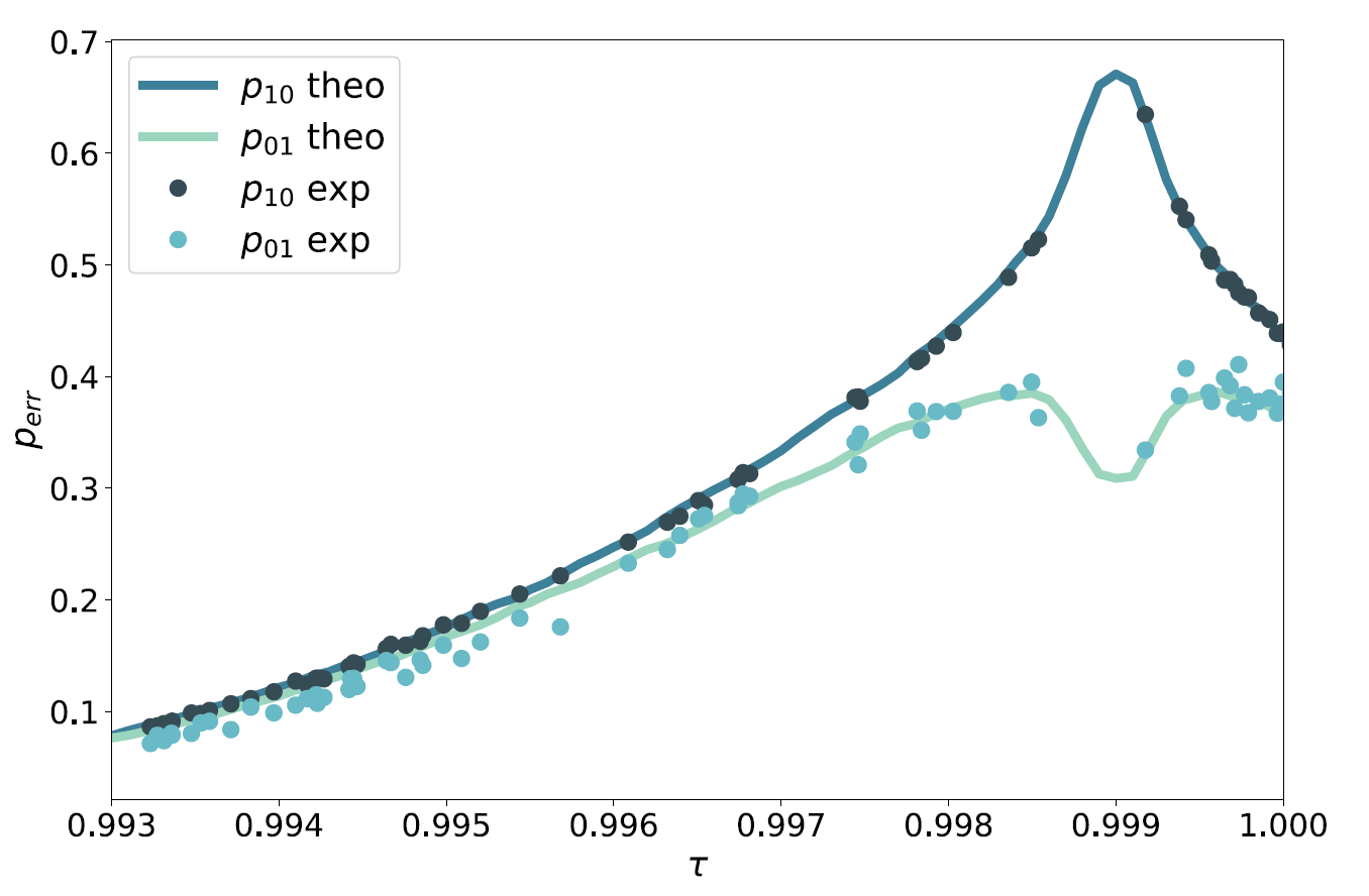
The false positive and negative probabilities of the quantum PC strategy can be evaluated experimentally with the same procedure as the one described in the Materials and Methods for the total probability of error. The experimental points, along with the theoretical curves are reported in Fig.(6).

The experiment is based on spontaneous parametric down-conversion and is depicted in Fig.(7). A multi-mode TMSV state $\otimes^{K}|\psi\rangle$ is generated using a 1 cm³ type-II $\beta$-barium borate (BBO) crystal and a continuous-wave laser at $\lambda_{p}=405$ nm, delivering a power of 100 mW. The down-converted photons are correlated in momentum. This correlation is mapped into spatial correlations using a lens in $f$-$f$ configuration: the “far-field” lens ($f_{\text{FF}}=1$ cm) is positioned at one focal length of the output plane of the crystal. The absorption sample is positioned in the conjugated plane, which corresponds to the far-field of the source. It consists of a coated glass plate, which presents different transmittance regions, realized with depositions of varying density. A blank coated glass is inserted in the idler beam’s path, to match the optical paths of both beams. The sample is imaged using a second “imaging” lens onto a charge-coupled (CCD) camera (Princeton Instruments PIXIS:400BR eXcellon), working in linear mode, with high quantum efficiency ($>95\%$ at 810 nm) and low (few electrons per pixel per frame) electronic noise. Individual pixels of the camera are binned together in 12x12 macro-pixels, to increase the readout signal-to-noise ratio and the acquisition speed.

The photon counts $n_{S}$ and $n_{I}$ of the signal and idler beams are obtained by integrating over two spatially correlated detection areas $\mathrm{S}_{S}$ and $\mathrm{S}_{I}$, which are sub-parts of the “full” correlated areas. The two “full” correlated areas are schematically defined by the two illuminated regions on the camera, i.e. the spatial extent of the idler and signal beams. Their precise definition is made using a procedure described in Samantaray et al. 2017. The total number of spatial modes collected is $K_{s}\sim 10^{3}$, and that of temporal mode is $K_{t}\sim 10^{10}$ (see Brida et al. 2010 for more details on the estimation). The mean photon number measured in one region $S_{i}$ is $\bar{n}_{i}\sim 10^{5}$. Hence, the mean occupation number per mode is very small $\bar{n}_{i}/(K_{s}\times K_{t})\sim 10^{-8}$. Under these conditions, the multi-thermal marginal photon-number distributions can be well approximated by Poisson distributions Mandel and Wolf 1995. When the absorptive sample is replaced with an equivalent coated glass plate without any deposition, we estimate, for each pair of regions $\mathrm{S}_{S}$ and $\mathrm{S}_{I}$, the corresponding detection efficiencies $\eta_{S}$ and $\eta_{I}$, by exploiting the correlations of the SPDC process Meda et al. 2014; Brida et al. 2006. Indeed, the phase matching conditions, the interference filter, the quality of the optical alignment, and the pixels’ properties on the camera all introduce small differences in the photon number correlations that need to be accounted for. With the absorptive sample, for each pair of regions, i.e. for all the different values of $\tau$, $N_{\mathcal{D}_{\tau}}=2\cdot 10^{4}$ frames are recorded ($\mathcal{D}_{\tau}$ designates the experimental dataset for transmittance $\tau$).

Using the experimental data, two error probabilities, $p_{01}$ and $p_{10}$, must be evaluated to access to the total error probability:

$$p_{err}=\frac{1}{2}\left(p_{01}+p_{10}\right).$$

(18)

In our analysis, the reference process $\mathcal{P}_{0}$ is strongly peaked around $\tau_{0}$. Hence, the evaluation of $p_{10}$ with experimental data is rather straightforward. We use the dataset $\mathcal{D}_{\tau_{0}}$, composed of $M$ measurement outcome $(n_{s};n_{i})$, when the transmittance $\tau_{0}$ is inserted in the signal branch, to compute the experimental frequency of error $f_{10}$. In particular, for each data pair $(n_{s};n_{i})\in\mathcal{D}_{\tau_{0}}$, a label $y\in\{0,1\}$ is assigned according to the maximum likelihood strategy described in the main text. In the evaluation, experimental parameters, such as the mean photon number of the source and the detection efficiencies are used, estimated in a calibration phase. $f_{10}$ is then defined as the number of wrong decisions, which in this case is simply the number of occurrences of $y=1$ over $M$. $f_{10}$ will converge to the real probability of error $p_{10}$ as the number of experimental points in the dataset $M$ becomes large.

On the other hand, the evaluation of $p_{01}$ requires a more careful approach. In fact, one has to construct an ensemble of experimental data $\mathcal{D}_{\mathcal{P}_{1}}$, whose data are taken with parameters $\tau$ distributed in a way that is representative of the true probability density $g_{1}(\tau)$. Experimentally, we acquire $\bar{M}$ photon number pairs for each of the transmittance $\tau_{i},\;i\in\{1,...,L\}$, i.e. $\bar{M}\cdot L$ data points in total. The transmittance values $\tau_{i}$ are selected in an interval $[\tau_{min},\tau_{max}]$. They may not be distributed uniformly in this interval, because of a non perfect experimental control of the position of the absorption layer, and the uncertainty on the estimation of $\tau_{i}$. Starting from the experimental dataset, and binning the interval $[\tau_{min},\tau_{max}]$ in $K$ equal sub-intervals of size $2l$ ($2l=(\tau_{max}-\tau_{min})/K$), we define the experimental distribution for the transmittance, $g$, as the normalized histogram

$$g(\tau)=\sum_{k=1}^{K}\frac{d_{k}}{2lL}\Theta_{k}\left(\tau\right),$$

(19)

where $d_{k}$ is the number of experimental transmittance values $\tau_{i}$ that fall in the $k$-th bin, so that the relative number of pairs $(n_{s};n_{i})_{k}$ is $d_{k}\bar{M}$. $\Theta_{k}\left(\tau\right)$ is a step function, equal to unity in the $k$-th bin and 0 elsewhere. In an ideal case, the experimental distribution $g$ in Eq.(19), should be a uniform distribution in the interval $[\tau_{min},\tau_{max}]$, but, in practice, because of the experimental issues mentioned above, it can present significant discrepancies with respect to it.

In order to approximate a general probability distribution $f(t)$, we can multiply the coefficients in Eq. (19), by proper weights $w_{k}$, with $k\in\{1,...,K\}$. Once the weights are determined by a proper optimization procedure, described in the Supplementary Materials, they are used to modulate the number of experimental data in each bin according to the substitution $d_{k}\bar{M}\longmapsto d_{k}w_{k}\bar{M}$. $w_{k}$ represents the fraction of data kept in bin $k$. The ensemble of data randomly picked from the initial set, according to the weights, will define the final set $\mathcal{D}_{\mathcal{P}_{1}}$. We refer to the distribution of $\mathcal{D}_{\mathcal{P}_{1}}$ after the reweighting procedure, as $g_{\mathbf{w}}(\tau)$, where $\mathbf{w}=[w_{1},...,w_{K}]$. Since the experimental set cannot be increased, the constraint $0\leq w_{k}\leq 1$ must be imposed. The procedure will in general reduce the number of points in the dataset: an increase of the statistical uncertainty can arise. Thus, it may be useful to introduce a second constraint on the size of the final dataset, $M_{T}=\sum_{k=1}^{K}d_{k}w_{k}\bar{M}$, in the optimization procedure to put a lower bound on how much data is discarded.

For the optimization process, we define the objective function to be maximized as the Bhattacharyya coefficient between the distributions $f$ and $g_{\mathbf{w}}$:

$$T\left(\mathbf{w}\right)=\int_{\tau_{min}}^{\tau_{max}}\sqrt{f(\tau)g_{\mathbf{w}}(\tau)}d\tau.$$

(20)

This quantity measures their similarity and ranges between 0 and 1. $T\left(\mathbf{w}\right)$ gives a quantitative measure of how close the experimental dataset can be arranged to resemble the objective distribution. We define a threshold value $0\leq T_{th}\leq 1$, above which the approximation of $f\approx g_{\mathbf{w}}$ is deemed “good enough”, i.e. $T\left(\mathbf{w}\right)\geq T_{th}$. In general, the optimal $\mathbf{w}$ and the corresponding $T\left(\mathbf{w}\right)$, depend on the interval $[\tau_{min};\tau_{max}]$, which should be chosen so that $\int_{\tau_{min}}^{\tau_{max}}f(t)$ is close to unity. We note that the minimum number of data points $M_{T}$ and the initial distribution of the experimental data can affect the results of the optimization algorithm. For this reason, in our realization of this algorithm, we sampled the interval $[\tau_{min},\tau_{max}]$ with a dense array of values $\tau_{i}$, taken equispaced within the experimental uncertainty, and we took a very large total number of data points with respect to the target $M_{T}$. The approximated distribution for the data, reported in the Results section, had a coefficient $T\sim 1$. A more formal description, as well as further details on the procedure, are reported in the Supplementary Materials.

This work was founded by the EU via “Quantum readout techniques and technologies” (QUARTET, Grant agreement No 862644).

GO and IRB proposed the QCT protocol. GO developed the theoretical model and performed the theoretical and numerical analysis both for the classical limits and the quantum protocol. PB and EL acquired the experimental data, the experiment being designed by IRB. PB and GO performed the data analysis, with contributions from IPD. MG leads the quantum optics group at INRiM and coordinated the project. All authors contributed to the discussion of the results and the writing of the manuscript.

The authors declare no competing interest.

All data needed to evaluate the conclusions are reported in the paper. Further data are available under reasonable request to the corresponding author.

We consider first a scenario in which only the defective process $\mathcal{P}_{1}$ is distributed according to some arbitrary distribution $g_{1}(\tau)$, while the reference process $\mathcal{P}_{0}$ is strongly peaked, i.e. it can be assumed that all the object produced have the same trasmittance parameter $\tau_{0}$. In this situation, for any classical input state $\rho_{cla}$, as defined in the main text, using the strong convexity of the trace distance, we can write:

		$\displaystyle D(\rho_{0},\rho_{1})\leq\int d^{\text{\tiny$2M$}}\bm{\alpha}\;d^{\text{\tiny$2L$}}\bm{\beta}\;P(\bm{\alpha},\bm{\beta})\times$
		$\displaystyle\times D(\mathcal{E}_{\tau_{0}}(|\bm{\alpha}\rangle\langle\bm{\alpha}|)\otimes|\bm{\beta}\rangle\langle\bm{\beta}|,\mathbb{E}_{\mathcal{P}_{1}}[\mathcal{E}_{\tau}(|\bm{\alpha}\rangle\langle\bm{\alpha}|)]\otimes|\bm{\beta}\rangle\langle\bm{\beta}|)$
		$\displaystyle=\int d^{\text{\tiny$2M$}}\bm{\alpha}\,P(\bm{\alpha})D(\mathcal{E}_{\tau_{0}}(|\bm{\alpha}\rangle\langle\bm{\alpha}|),\mathbb{E}_{\mathcal{P}_{1}}[\mathcal{E}_{\tau}(|\bm{\alpha}\rangle\langle\bm{\alpha}|)]),$		(S.2)

where $\mathbb{E}_{\mathcal{P}_{1}}$ is the expectation value over the distribution $g_{1}(\tau)$ and the last equality follows from the fact that the unaffected reference system doesn’t change the trace distance. Using once again the convexity of the trace on the second argument of the integrating term $D$, we have:

		$\displaystyle D(\mathcal{E}_{\tau_{0}}(|\bm{\alpha}\rangle\langle\bm{\alpha}|),\mathbb{E}_{\mathcal{P}_{1}}[\mathcal{E}_{\tau}(|\bm{\alpha}\rangle\langle\bm{\alpha}|)])$
		$\displaystyle\leq\mathbb{E}_{\mathcal{P}_{1}}[D(\mathcal{E}_{\tau_{0}}(|\bm{\alpha}\rangle\langle\bm{\alpha}|),\mathcal{E}_{\tau}(|\bm{\alpha}\rangle\langle\bm{\alpha}|))]$
		$\displaystyle=\mathbb{E}_{\mathcal{P}_{1}}[D(|\sqrt{\tau_{0}}\bm{\alpha}\rangle\langle\sqrt{\tau_{0}}\bm{\alpha}|,|\sqrt{\tau}\bm{\alpha}\rangle\langle\sqrt{\tau}\bm{\alpha}|)]$		(S.3)

To derive this expression, we used the fact that pure loss channels map coherent states into coherent states, i.e. $|\alpha\rangle\xrightarrow{\mathcal{E_{\tau}}}|\sqrt{\tau}\alpha\rangle$. The distance between two pure states is easily calculated:

	$\displaystyle D\left(|\sqrt{\tau_{0}}\bm{\alpha}\rangle,|\sqrt{\tau}\bm{\alpha}\rangle\right))$	$\displaystyle=\sqrt{1-F(|\sqrt{\tau_{0}}\bm{\alpha}\rangle,|\sqrt{\tau}\bm{\alpha}\rangle)^{2}}$
		$\displaystyle=\sqrt{1-e^{-|\bm{\alpha}|^{2}(\sqrt{\tau_{0}}-\sqrt{\tau})^{2}}}$		(S.4)

with $F(\cdot,\cdot)$ is the fidelity between two quantum states. We can then write:

$$D\left(\rho_{0},\rho_{1}\right)\leq\mathbb{E}_{\mathcal{P}_{1}}\Bigg[\int d^{\text{\tiny$2M$}}\bm{\alpha}\,P(\bm{\alpha})\sqrt{1-e^{-|\bm{\alpha}|^{2}(\sqrt{\tau_{0}}-\sqrt{\tau})^{2}}}\Bigg]$$

(S.5)

Given the condition on the total number of photons on the signal system $N_{S}$ in Eq.(5) of the main text, we have (see Supplementary Materials of Ref.Pirandola 2011):

	$\displaystyle\int d^{\text{\tiny$2M$}}\bm{\alpha}\,P(\bm{\alpha})$	$\displaystyle\sqrt{1-e^{-|\bm{\alpha}|^{2}(\sqrt{\tau_{0}}-\sqrt{\tau})^{2}}}$
		$\displaystyle\leq\sqrt{1-e^{-N(\sqrt{\tau_{0}}-\sqrt{\tau})^{2}}}$		(S.6)

for any probability distribution $P(\bm{\alpha})$.
Using Eq.(S.1), we can now lower bound the minimum probability of error in the QCT protocol, when one of the processes is strongly peaked, as:

$$p_{err}^{cla}\geq\frac{1-\mathbb{E}_{\mathcal{P}_{1}}\big[\sqrt{1-e^{-\bar{n}_{s}(\sqrt{\tau_{0}}-\sqrt{\tau})^{2}}}\big]}{2}$$

(S.7)

If we relax the condition of strongly peaked reference process, so that $\mathcal{P}_{0}$ is distributed as $g_{0}(\tau_{0})$, we have in place of Eq.(S.3), using the convexity on both arguments:

		$\displaystyle D(\mathbb{E}_{\mathcal{P}_{0}}[\mathcal{E}_{\tau}(|\bm{\alpha}\rangle\langle\bm{\alpha}|)],\mathbb{E}_{\mathcal{P}_{1}}[\mathcal{E}_{\tau}(|\bm{\alpha}\rangle\langle\bm{\alpha}|)])\leq$
		$\displaystyle\mathbb{E}_{\mathcal{P}_{0}}\mathbb{E}_{\mathcal{P}_{1}}[D(\mathcal{E}_{\tau_{0}}(|\bm{\alpha}\rangle\langle\bm{\alpha}|),\mathcal{E}_{\tau_{1}}(|\bm{\alpha}\rangle\langle\bm{\alpha}|))]=$
		$\displaystyle=\mathbb{E}_{\mathcal{P}_{0}}\mathbb{E}_{\mathcal{P}_{1}}[D(|\sqrt{\tau_{0}}\bm{\alpha}\rangle\langle\sqrt{\tau_{0}}\bm{\alpha}|,|\sqrt{\tau_{1}}\bm{\alpha}\rangle\langle\sqrt{\tau_{1}}\bm{\alpha}|)]$		(S.8)

So that repeating the steps of previous section the probability of success will be given by

$$p_{err}^{cla}\geq\frac{1-\mathbb{E}_{\mathcal{P}_{0}}\mathbb{E}_{\mathcal{P}_{1}}\big[\sqrt{1-e^{-N(\sqrt{\tau_{0}}-\sqrt{\tau_{1}})^{2}}}\big]}{2},$$

(S.9)

That is Eq.(7) of the main text

We consider the case in which both the processes distributions have Gaussian form with mean $\bar{\tau}_{x}$ and variance $\sigma_{x}^{2}$, i.e. $g_{x}(\tau)=G_{\bar{\tau}_{x},\sigma_{x}}(\tau)$. According to Eq.(S.14-S.15), we have for the final photon number distribution, $h^{(x)}_{G}(n)$:

	$\displaystyle N_{G}^{(x)}$	$\displaystyle=\mathbb{E}_{h}[n]={\bar{n}_{s}}\bar{\tau}_{x}$		(S.16)
	$\displaystyle\sigma_{G}^{(x)}$	$\displaystyle=var_{h}[n]={\bar{n}_{s}}\bar{\tau}_{x}+{\bar{n}_{s}}^{2}\sigma_{x}^{2}$		(S.17)

For ${\bar{n}_{s}}$ large enough, the distribution $h_{G}(n)$ will converge to a gaussian itself:

$$h^{(x)}_{G}(n)\sim G(n,N_{G},\sigma_{G})\qquad\qquad\qquad{\bar{n}_{s}}>>0$$

(S.18)

In this approximation the probability of error of the procedure can be evaluated according to Eq.(S.11) and (S.13) as:

	$\displaystyle p_{err}$	$\displaystyle=\frac{1}{2}\Bigg(\sum_{\{n|y=1\}}p(n|\mathcal{P}_{0})+\sum_{\{n|y=0\}}p(n|\mathcal{P}_{1})\Bigg)$
		$\displaystyle\approx\frac{1}{2}\Bigg(\int_{\{n|y=1\}}G_{N^{(0)}_{G},\sigma^{(0)}_{G}}(n)+\int_{\{n|y=0\}}G_{N^{(1)}_{G},\sigma^{(1)}_{G}}(n)\Bigg)$		(S.19)

when used the assumption ${\bar{n}_{s}}>>0$ in Eq.(S.18) to approximate the the sums with integrals over $n$.

To determine the regions of integration, we impose the condition $G_{N^{(0)}_{G},\sigma^{(0)}_{G}}(n)=G_{N^{(1)}_{G},\sigma^{(1)}_{G}}(n)$. This condition defines up to two threshold values, $n_{th}$, for $n$, whose expression, if $\sigma_{G}^{(0)}\neq\sigma_{G}^{(1)}$, is:

	$\displaystyle n_{th}^{(-)}$	$\displaystyle=\frac{N_{G}^{(0)}(\sigma_{G}^{(1)})^{2}-N_{G}^{(1)}(\sigma_{G}^{(0)})^{2}-\sqrt{(\sigma_{G}^{(0)}\sigma_{G}^{(1)})^{2}\left(2\left(\sigma_{G}^{(1)}-\sigma_{G}^{(0)}\right)\left(\sigma_{G}^{(1)}+\sigma_{G}^{(0)}\right)\left(\log\left(\sigma_{G}^{(1)}\right)-\log\left(\sigma_{G}^{(0)}\right)\right)+\left(N_{G}^{(1)}-N_{G}^{(0)}\right)^{2}\right)}}{\left(\sigma_{G}^{(1)}-\sigma_{G}^{(0)}\right)\left(\sigma_{G}^{(1)}+\sigma_{G}^{(0)}\right)}$
	$\displaystyle n_{th}^{(+)}$	$\displaystyle=\frac{N_{G}^{(0)}(\sigma_{G}^{(1)})^{2}-N_{G}^{(1)}(\sigma_{G}^{(0)})^{2}+\sqrt{(\sigma_{G}^{(0)}\sigma_{G}^{(1)})^{2}\left(2\left(\sigma_{G}^{(1)}-\sigma_{G}^{(0)}\right)\left(\sigma_{G}^{(1)}+\sigma_{G}^{(0)}\right)\left(\log\left(\sigma_{G}^{(1)}\right)-\log\left(\sigma_{G}^{(0)}\right)\right)+\left(N_{G}^{(1)}-N_{G}^{(0)}\right)^{2}\right)}}{\left(\sigma_{G}^{(1)}-\sigma_{G}^{(0)}\right)\left(\sigma_{G}^{(1)}+\sigma_{G}^{(0)}\right)}$

and, if $\sigma_{G}^{(0)}=\sigma_{G}^{(1)}$:

$$n_{th}^{(0)}=\frac{\mu_{1}+\mu_{2}}{2}$$

(S.21)

We consider the first case, i.e. $\sigma_{G}^{(0)}\neq\sigma_{G}^{(1)}$, assuming, without loss of generality, $\sigma_{G}^{(1)}>\sigma_{G}^{(0)}$, we have $n_{th}^{(+)}>n_{th}^{(-)}$, and the value $y=1$ will be selected if $n>n_{th}^{(+)}$ or $n<n_{th}^{(-)}$. We have:

	$\displaystyle p_{err}\approx\frac{1}{2}\Bigg($	$\displaystyle\int_{-\infty}^{n_{th}^{(-)}}G_{N_{G}^{(0)},\sigma_{G}^{(0)}}(n)+\int^{n_{th}^{(+)}}_{n_{th}^{(-)}}G_{N_{G}^{(1)},\sigma_{G}^{(1)}}(n)+$
	$\displaystyle+$	$\displaystyle\int^{\infty}_{n_{th}^{(+)}}G_{N_{G}^{(0)},\sigma_{G}^{(0)}}(n)\Bigg)$		(S.22)

when we note how the first integral should run from $0$ rather than $-\infty$ but since we are considering ${\bar{n}_{s}}>>0$ we can approximate the exact range of integration with the latter ($n_{th}^{(-)}$ can take also negative values but in that case the integral will not contribute to $p_{err}$). Defining:

$\displaystyle E^{x}(n_{th})=\text{erf}\Big[\frac{n_{th}-N_{G}^{(x)}}{\sqrt{2}\sigma_{G}^{(x)}}\Big]$

(S.23)

Where erf$(x)$ is the error function. We have:

	$\displaystyle p_{err}$	$\displaystyle\approx\frac{1}{2}\Big(1-q_{G}\Big)$		(S.24)
	$\displaystyle q_{G}$	$\displaystyle:=\frac{1}{2}\Big(E^{0}(n_{th}^{(+)})+E^{1}(n_{th}^{(-)})-E^{0}(n_{th}^{(-)})-E^{1}(n_{th}^{(+)})\Big)$		(S.25)

To simplify the expression above, we note how, if $\sigma_{G}^{(0)}\approx\sigma_{G}^{(1)}$ one of the threshold values will be far from the center of both distributions so that it can be neglected and the solution can be considered unique. In particular, we can define:

	$\displaystyle q_{G}^{(+)}({\bar{n}_{s}},\tau_{0},\bar{\tau},\sigma):=$	$\displaystyle\frac{1}{2}\Bigg(E^{0}(n_{th}^{(+)})-E^{1}(n_{th}^{(+)}\Bigg)$		(S.26)
	$\displaystyle q_{G}^{(-)}({\bar{n}_{s}},\tau_{0},\bar{\tau},\sigma):=$	$\displaystyle\frac{1}{2}\Bigg(E^{1}(n_{th}^{(-)})-E^{0}(n_{th}^{(-)})\Bigg)$		(S.27)

and in the approximation of similar variances, we have:

References

- Pirandola et al. (2018) S. Pirandola, B. R. Bardhan, T. Gehring, C. Weedbrook, and S. Lloyd, Advances in photonic quantum sensing, Nature Photonics 12, 724 (2018).
- Degen et al. (2017) C. L. Degen, F. Reinhard, and P. Cappellaro, Quantum sensing, Reviews of Modern Physics 89, 035002 (2017).
- Genovese (2016) M. Genovese, Real applications of quantum imaging, Journal of Optics 18, 073002 (2016).
- Berchera and Degiovanni (2019) I. R. Berchera and I. P. Degiovanni, Quantum imaging with sub-poissonian light: challenges and perspectives in optical metrology, Metrologia 56, 024001 (2019).
- Polino et al. (2020) E. Polino, M. Valeri, N. Spagnolo, and F. Sciarrino, Photonic quantum metrology, AVS Quantum Science 2, 024703 (2020).
- Helstrom (1976) C. Helstrom, Quantum detection and estimation theory (Academic Press, New York, 1976).
- Chefles and Barnett (1998) A. Chefles and S. M. Barnett, Quantum state separation, unambiguous discrimination and exact cloning, Journal of Physics A: Mathematical and General 31, 10097 (1998).
- Chefles (2000) A. Chefles, Quantum state discrimination, Contemporary Physics 41, 401 (2000).
- Aasi et al. (2013) J. Aasi et al., Enhanced sensitivity of the ligo gravitational wave detector by using squeezed states of light, Nature Photonics 7, 613 EP (2013).
- Ruo Berchera et al. (2013) I. Ruo Berchera, I. P. Degiovanni, S. Olivares, and M. Genovese, Quantum light in coupled interferometers for quantum gravity tests, Physical Review Letter 110, 213601 (2013).
- Schäfermeier et al. (2018) C. Schäfermeier, M. Ježek, L. S. Madsen, T. Gehring, and U. L. Andersen, Deterministic phase measurements exhibiting super-sensitivity and super-resolution, Optica 5, 60 (2018).
- Ortolano et al. (2019) G. Ortolano, I. Ruo-Berchera, and E. Predazzi, Quantum enhanced imaging of nonuniform refractive profiles, International Journal of Quantum Information 17, 1941010 (2019).
- Pradyumna et al. (2020) S. T. Pradyumna, E. Losero, I. Ruo-Berchera, P. Traina, M. Zucco, C. S. Jacobsen, U. L. Andersen, I. P. Degiovanni, M. Genovese, and T. Gehring, Twin beam quantum-enhanced correlated interferometry for testing fundamental physics, Communications Physics 3, 104 (2020).
- Tapster et al. (1991) P. R. Tapster, S. F. Seward, and J. G. Rarity, Sub-shot-noise measurement of modulated absorption using parametric down-conversion, Physical Review A 44, 3266 (1991).
- Monras and Paris (2007) A. Monras and M. G. A. Paris, Optimal quantum estimation of loss in bosonic channels, Physical Review Letter 98, 160401 (2007).
- Adesso et al. (2009) G. Adesso, F. Dell’Anno, S. De Siena, F. Illuminati, and L. A. M. Souza, Optimal estimation of losses at the ultimate quantum limit with non-gaussian states, Physical Review A 79, 040305 (2009).
- Matthews et al. (2016) J. C. Matthews, X.-Q. Zhou, H. Cable, P. J. Shadbolt, D. J. Saunders, G. A. Durkin, G. J. Pryde, and J. L. O’Brien, Towards practical quantum metrology with photon counting, npj Quantum Information 2, 16023 (2016).
- Moreau et al. (2017) P.-A. Moreau, J. Sabines-Chesterking, R. Whittaker, S. K. Joshi, P. M. Birchall, A. McMillan, J. G. Rarity, and J. C. F. Matthews, Demonstrating an absolute quantum advantage in direct absorption measurement, Scientific Reports 7, 6256 (2017).
- Losero et al. (2018) E. Losero, I. Ruo-Berchera, A. Meda, A. Avella, and M. Genovese, Unbiased estimation of an optical loss at the ultimate quantum limit with twin-beams, Scientific Reports 8, 7431 (2018).
- Avella et al. (2016) A. Avella, I. Ruo-Berchera, I. P. Degiovanni, G. Brida, and M. Genovese, Absolute calibration of an emccd camera by quantum correlation, linking photon counting to the analog regime, Optics Letter 41, 1841 (2016).
- Brida et al. (2010) G. Brida, M. Genovese, and I. Ruo Berchera, Experimental realization of sub-shot-noise quantum imaging, Nature Photonics 4, 227 (2010).
- Samantaray et al. (2017) N. Samantaray, I. Ruo-Berchera, A. Meda, and M. Genovese, Realization of the first sub-shot-noise wide field microscope, Light: Science & Applications 6, e17005 EP (2017).
- Sabines-Chesterking et al. (2019) J. Sabines-Chesterking, A. R. McMillan, P. A. Moreau, S. K. Joshi, S. Knauer, E. Johnston, J. G. Rarity, and J. C. F. Matthews, Twin-beam sub-shot-noise raster-scanning microscope, Optics Express 27, 30810 (2019).
- Lloyd (2008) S. Lloyd, Enhanced sensitivity of photodetection via quantum illumination, Science 321, 1463 (2008).
- Tan et al. (2008) S.-H. Tan, B. I. Erkmen, V. Giovannetti, S. Guha, S. Lloyd, L. Maccone, S. Pirandola, and J. H. Shapiro, Quantum illumination with gaussian states, Physical Review Letter 101, 253601 (2008).
- Lopaeva et al. (2013) E. D. Lopaeva, I. Ruo Berchera, I. P. Degiovanni, S. Olivares, G. Brida, and M. Genovese, Experimental realization of quantum illumination, Physical Review Letter 110, 153603 (2013).
- Zhang et al. (2015) Z. Zhang, S. Mouradian, F. N. C. Wong, and J. H. Shapiro, Entanglement-enhanced sensing in a lossy and noisy environment, Physical Review Letter 114, 110506 (2015).
- Pirandola (2011) S. Pirandola, Quantum reading of a classical digital memory, Physical Review Letter 106, 090504 (2011).
- Ortolano et al. (2021) G. Ortolano, E. Losero, S. Pirandola, M. Genovese, and I. Ruo-Berchera, Experimental quantum reading with photon counting, Science Advances 7, eabc7796 (2021).
- Pendrill (2014) L. R. Pendrill, Using measurement uncertainty in decision-making and conformity assessment, Metrologia 51, S206 (2014).
- Nielsen and Chuang (2011) M. A. Nielsen and I. L. Chuang, Quantum Computation and Quantum Information, 10th ed. (Cambridge University Press, USA, 2011).
- Meda et al. (2017) A. Meda, E. Losero, N. Samantaray, F. Scafirimuto, S. Pradyumna, A. Avella, I. Ruo-Berchera, and M. Genovese, Photon-number correlation for quantum enhanced imaging and sensing, Journal of Optics 19, 094002 (2017).
- Pirandola et al. (2011) S. Pirandola, C. Lupo, V. Giovannetti, S. Mancini, and S. L. Braunstein, Quantum reading capacity, New Journal of Physics 13, 113012 (2011).
- Mandel and Wolf (1995) L. Mandel and E. Wolf, Optical Coherence and Quantum Optics (Cambridge University Press, 1995).
- Weedbrook et al. (2012) C. Weedbrook, S. Pirandola, R. García-Patrón, N. J. Cerf, T. C. Ralph, J. H. Shapiro, and S. Lloyd, Gaussian quantum information, Reviews of Modern Physics 84, 621 (2012).
- Bondani et al. (2007) M. Bondani, A. Allevi, G. Zambra, M. G. A. Paris, and A. Andreoni, Sub-shot-noise photon-number correlation in a mesoscopic twin beam of light, Physical Review A 76, 013833 (2007).
- Peřina et al. (2007) J. Peřina, J. Křepelka, J. Peřina, M. Bondani, A. Allevi, and A. Andreoni, Experimental joint signal-idler quasidistributions and photon-number statistics for mesoscopic twin beams, Physical Review A 76, 043806 (2007).
- Chekhova et al. (2018) M. V. Chekhova, S. Germanskiy, D. B. Horoshko, G. K. Kitaeva, M. I. Kolobov, G. Leuchs, C. R. Phillips, and P. A. Prudkovskii, Broadband bright twin beams and their upconversion, Optics Letter 43, 375 (2018).
- Glorieux et al. (2011) Q. Glorieux, L. Guidoni, S. Guibal, J.-P. Likforman, and T. Coudreau, Quantum correlations by four-wave mixing in an atomic vapor in a nonamplifying regime: Quantum beam splitter for photons, Physical Review A 84, 053826 (2011).
- Pooser and Lawrie (2016) R. C. Pooser and B. Lawrie, Plasmonic trace sensing below the photon shot noise limit, ACS Photonics 3, 8 (2016).
- Wu et al. (2019) M.-C. Wu, B. L. Schmittberger, N. R. Brewer, R. W. Speirs, K. M. Jones, and P. D. Lett, Twin-beam intensity-difference squeezing below 10 hz, Optics Express 27, 4769 (2019).
- Brida et al. (2010) G. Brida, I. Degiovanni, M. Genovese, M. L. Rastello, and I. Ruo-Berchera, Detection of multimode spatial correlation in pdc and application to the absolute calibration of a ccd camera, Optics Express 18, 20572 (2010).
- Meda et al. (2014) A. Meda, I. Ruo-Berchera, I. P. Degiovanni, G. Brida, M. L. Rastello, and M. Genovese, Absolute calibration of a charge-coupled device camera with twin beams, Applied Physics Letters 105, 101113 (2014).
- Brida et al. (2006) G. Brida, M. Genovese, I. Ruo-Berchera, M. Chekhova, and A. Penin, Possibility of absolute calibration of analog detectors by using parametric downconversion: a systematic study, Journal of the Optical Society of America B 23, 2185 (2006).
Supplementary Materials
V Derivation of the classical limit
In this section, we show how the bound in Eq.(7) of the main text can be derived. is a bound on the minimum probability of error, in the QCT protocol, achievable using as probe classical states – as defined in the main text –, , with fixed signal energy .
Given an input state , the output state, after interaction with the SUT, will be either or . The best performance in discriminating between those states is achieved by using a POVM measurement, which assumes the Helstrom projectors as elements Helstrom 1976, yielding a probability of error: