Closed-Form Parametric Equation for the
Minkowski Sum of Ellipsoids in
and Associated Volume Bounds
Gregory S. Chirikjian
Department of Mechanical Engineering
National University of Singapore
mpegre@nus.edu.sg
and
Department of Mechanical Engineering
Johns Hopkins University
gchirik1@jhu.edu
Bernard Shiffman
Department of Mathematics
Johns Hopkins University
bshiffman@jhu.edu
March 18, 2021
Abstract
General results on convex bodies are reviewed and used to derive an exact closed-form parametric formula for the Minkowski sum boundary of arbitrary ellipsoids in -dimensional Euclidean space. Expressions for the principal curvatures of these Minkowski sums are also derived. These results are then used to obtain upper and lower volume bounds for the Minkowski sum of ellipsoids in terms of their defining matrices; the lower bounds are sharper than the Brunn-Minkowski inequality. A reverse isometric inequality for convex bodies is also given.
1 Introduction
The concept of the Minkowski sum of two bodies in -dimensional Euclidean space is fundamental in the field of convex geometry. When , Minkowski sums play important roles in applied fields such as robot motion planning, computational chemistry, and computer graphics [5, 6, 8, 17, 18, 20, 23, 27].
By a body we mean a bounded, connected, open (nonempty) subset of . (Note that our definition of a body differs from the literature where bodies are assumed to be compact rather than open and bounded.) Given two such bodies, and , their Minkowski sum is defined by
| (1) |
Among all convex bodies with differentiable boundaries, ‘solid ellipsoids’ of the form , where is a nonsingular matrix, constitute a fairly broad, yet simple, class of objects. Solid ellipsoids are convenient since their boundaries have both closed form parametric and implicit descriptions. The ellipsoid can be parameterized as
| (2) |
where (the unit sphere) is a unit vector, and are spherical angles (or any local coordinates) that parameterize the sphere.
The corresponding implicit equation of is
| (3) |
We note that is a positive-definite symmetric matrix, and the ellipsoid can be reparameterized as
| (4) |
When using (4), the unit normal to at is computed as
| (5) |
Since this means that is a scalar multiple of , it is possible to invert the above expression as
| (6) |
| (7) |
which confirms the bijectivity of the Gauss map for ellipsoids. (The Gauss map from the boundary of a convex body is always bijective onto .) When using (2) with a nonsymmetric matrix , the equation corresponding to (5) is
| (8) |
In [27], the procedure to generate the Minkowski sum boundary for solid ellipsoids and (defined by symmetric matrices and ) was to morph space so as to compute
where . Since this corresponds to an external surface offset relative to in the direction of the outward normal with a unit distance, then using (8) with gives the normal to the deformed ellipsoid, and the resulting offset surface is given parametrically by
Transforming back by multiplying by gives the result in [27]:
| (9) |
It is regrettable that even though . This led us to consider a new way of writing (9). Specifically, substituting (6) (with ) in equation (9) yields
| (10) |
Re-parametrizing (10) gives a new parametric formula for :
| (11) |
The first result of this paper is that is normal to and that this symmetric formula for the Minkowski sum boundary generalizes to ellipsoids:
Theorem 1.1.
Suppose that are solid ellipsoids in given by
where the are symmetric positive-definite matrices. Then the boundary of the Minkowski sum is given parametrically by
| (12) |
Furthermore, is the (outward-pointing) normal to the boundary of at .
We obtain Theorem 1.1 first as a special case of a general parametric formula for the Minkowski sum of convex bodies (Theorem 2.4) and then give an alternative computational derivation in Section 2.1.
We also have a formula for the principal curvatures of the boundary of the Minkowski sum of ellipsoids:
Theorem 1.2.
Let be the Minkowski sum of solid ellipsoids in given by symmetric positive-definite matrices as in Theorem 1.1, and let
| (13) |
Then is positive semidefinite of rank , and the principal curvatures of the Minkowski sum boundary at are the reciprocals of the positive eigenvalues of .
Indeed, we show that and that the self-adjoint operator is positive-definite on the hyperplane orthogonal to . In fact, is the Hessian matrix of the support function of the Minkowski sum .
We use the theory of general convex bodies in our proofs of Theorems 1.1 and 1.2. In our derivation of Theorem 1.1, we give a formula for the parametrization of the boundary of the Minkowski sum of convex bodies (Theorem 2.4). We also provide a reverse isometric inequality for convex bodies (Theorem 3.2).
2 Parametric equation for the Minkowski sum of strictly convex bodies
We begin by reviewing some basics about convex bodies. An important concept for the study of Minkowski sums of convex sets is the support function [14, 22]:
Definition 2.1.
The support function of a convex body is given by
Some elementary properties of the support function are:
- i)
,
- ii)
,
- iii)
,
- iv)
,
- v)
.
As a consequence of property (iv), two convex (open) bodies are identical if and only if their support functions are equal.
As an example, for a solid ellipsoid , where is positive definite symmetric, we have
| (14) |
It follows by property (i) of the support function that for the Minkowski sum of solid ellipsoids given as in Theorem 1.1, we have
| (15) |
Let be a convex body. By Theorem 4.1 of [14], for every , there exists such that
| (16) |
Now suppose that is strictly convex; i.e., for all pairs of points , the open line segment connecting and is contained in . Then for each , there is a unique satisfying (16). Thus we can define the normal parametrization of the boundary to be the map given by
| (17) |
Thus for a strictly convex body , the map is well-defined and surjective, but may not be injective (for example, if is piecewise smooth with corners). However, if is , then is injective and the parameter is the outward-pointing unit normal to at , since the maximum of on is attained at the point . In this case, is simply the inverse of the Gauss map
Example 2.2.
Without assuming smoothness of , we have the following:
Lemma 2.3.
[22, Lemma 2.2.12] If is a strictly convex body, then is continuous.
Proof.
The lemma is a consequence of the following fact: Let be a continuous function where and are Hausdorff spaces and is compact. For , let . Suppose that attains its maximum at a unique point for all . Then the map is continuous.
To prove this fact, let and let be an arbitrary neighborhood of . Then by compactness of and uniqueness of the maximum point. Therefore, there is a neighborhood of such that for all and hence for all , verifying that is continuous at .
We apply this with given by . Then is continuous.∎
Theorem 2.4.
Let be strictly convex bodies in . Then the normal parametrization of the boundary of the Minkowski sum is given by
| (19) |
Proof.
It suffices to consider the case . For , we have
The conclusion then follows from uniqueness of .∎
Proof of Theorem 1.1.
We give an alternative derivation of Theorem 1.1 in the following section.
2.1 Direct Proof of Theorem 1.1
The result holds for by (18). Using induction, we let and assume that the formula in (12) holds for . As in the proof of (9), we shall apply to and compute a normal offset.
The fact that is the outward-pointing unit normal to follows by an elementary computation. Specifically, if where are the spherical angles parametrizing the unit sphere (or are any local coordinates on the unit sphere), then a basis for the tangent hyperplane at the point on this surface will be the tangent vectors . These tangent vectors will be a sum over of
| (20) |
where
| (21) |
We note that for , we have
| (22) |
with equality if and only if . It follows that
| (23) |
Thus
and consequently
| (24) |
Hence, is the normal to .
It follows that is normal to . Therefore, the Minkowski sum of with the unit ball has boundary given parametrically as
The boundary of the Minkowski sum of ellipsoids is then given parametrically by
which is exactly the formula in (12) with .∎
3 Isoperimetric inequalities
The classical isoperimetric inequality gives a lower bound for the volume of the boundary of a bounded body :
| (25) |
Here denotes Lebesgue measure in , and
| (26) |
(This general isometric inequality is given in Federer [9, 3.2.43].) If is piecewise smooth, then is the usual -dimensional volume. In this case, (25) can be reduced to the case where is convex, where the result is a consequence of the Brunn-Minkowski inequality (see [12, 22]). More generally, if is ()-rectifiable, then , the Hausdorff ()-measure [9, 3.2.39]. Now let and denote the inradius and circumradius, respectively, of . Noting that
the isoperimetric inequality (25) immediately implies that
| (27) |
A sharper form of (27) is given by the following:
Theorem 3.1.
Let be the minimal volume outer ellipsoid (MVOE) of a bounded body in . Then
| (28) |
Theorem 3.1 is used in Section 5.3 to give an upper bound on the volume of the Minkowski sum of ellipsoids (Theorem 5.11).
Some reverse isometric inequalities for convex bodies based on affine transformations are given in [1] and [13]. We give here a reverse isometric inequality analogous to (27) and (28).
Theorem 3.2.
Let be a convex body. Then and
| (29) |
If is strictly convex or if is , then (29) is an equality if and only if is a ball.
Proof.
By a translation, we assume throughout this proof that .
We first consider the case where has a smooth boundary. By the divergence theorem,
| (30) |
Writing , for , we have
| (31) |
Therefore by (30),
| (32) |
verifying (29) for the case where is smooth.
Now suppose is not a ball and is . We must show strict inequality in (29). Since , there exists such that
Therefore is orthogonal to at , and hence . Thus, and hence strict equality holds in (32). This completes the argument that for smooth convex bodies , equality in (29) implies is a ball. The converse is trivial.
Now let be a general convex body. By [9, 3.2.35], is ()-rectifiable and hence [9, 3.2.39]. By [22, Theorem 2.2.6], is the intersection of half spaces, and therefore is the intersection of a decreasing sequence of convex polytopes . Since , it follows that the gradient (in the distribution sense) of the characteristic function of is a measure (i.e., has finite perimeter; see [10, p. 9]), and hence by a theorem of De Georgi [7] (see also [9, 4.5.6]), the divergence theorem (30) holds for with given by
| (33) |
for -a.a. . (By [9, 4.5.6] or [22, Theorem 2.2.5], there exists a unique satisfying (33) for -a.a. .) Then (29) follows from the divergence theorem as before.
Finally, we consider the case where is strictly convex and not necessarily smooth. Suppose that equation (29) is an equality. Then (31) is an equality for -a.a. . I.e., there exists a set such that and
| (34) |
Now fix a point . and let be the support hyperplane for through ; i.e., and is orthogonal to . Then by (34), is contained in the half-space , which is bounded by ; in particular . Let
We claim that . Indeed, suppose on the contrary that . Then by the strict convexity of , the midpoint , contradicting the fact that . Therefore and thus ; i.e. .
Since is arbitrary, we have shown that and therefore . Since , and all nonempty, relatively open subsets of have positive -measure zero, it follows that and thus . Therefore .∎
The inequality (29) for planar convex bodies () is stated in [21, p. 90]. Equality in (29) can occur for non-strictly-convex bodies, for example, when is an arbitrary triangle in , or when is an -cube in . In general, if equality holds in (29) for a convex body , then for every point , there exists a point such that the straight line segment from to is contained in (and is tangent to at ). To give another example, let be a cone in tangent to along a horizontal circle (with the vertex of below the sphere); then equality holds in (29) for the ‘ice cream cone’ shaped body bounded by the portion of below and the portion of above .
An alternative proof of (29) without geometric measure theory is as follows: As mentioned above, we can choose a decreasing sequence of convex polytopes , such that . We note that the divergence theorem (30) holds for convex polytopes (for an elementary proof, see [25, p. 10] or [26, Ch. III]), and (31) holds for all smooth points . It then follows as before that (29) holds for the polytopes . Since as , we have . Furthermore, for convex bodies ,
| (35) |
where is the projection onto the hyperplane in orthogonal to , and is the invariant probability measure on (see [12, 22]). It follows from (35) and the Lebesgue dominated convergence theorem that . Since , we have
Therefore,
∎
4 Differential Geometry of Strictly Convex Bodies: Proof of Theorem 1.2
In the following, we let be a convex body such that its boundary is and has strictly positive principal curvatures. This condition implies that is strictly convex (but strict convexity does not imply positive principal curvatures). We define by
| (36) |
where we recall that denotes the Gauss map of . We note that .
Lemma 4.1.
If is and has positive principal curvatures, then is on .
Proof.
If is , then the Gauss map is . Thus, it suffices to show that the Jacobian of is invertible at each point of and hence its inverse is . Let , and choose local coordinates on in a neighborhood of . Let be local coordinates on in a neighborhood of . We then can write
where denotes the point in with coordinates , and similarly denotes the point in with coordinates .
The Second Fundamental Form () for with respect to the coordinates is given by
| (37) |
where is the Jacobian of with respect to the coordinates and , and . If the principal curvatures of are non-zero, then is non-singular, and hence is non-singular.∎
We now use the notation .
Definition 4.2.
For as in Lemma 4.1 and , we define the convexity matrix by
| (38) |
where we write . I.e., is the Jacobian of at .
The following result is given in Schneider [22, p. 115]:
Lemma 4.3.
Proof.
To prove Theorem 1.2, we shall use the following result of Blaschke (in dimension 3) and Firey [11] (see also [22, Cor. 2.5.2]):
Theorem 4.4.
Let be a convex body such that its boundary is and has positive sectional curvatures. Then for all ,
- i)
is symmetric,
- ii)
,
- iii)
is positive-definite on ,
- iv)
the principal curvatures of the Minkowski sum boundary at are the reciprocals of the non-zero eigenvalues of .
Proof.
Conclusion (i) follows from (40). To verify (ii), we note that (38) implies that
Since , it follows that .
Let denote local coordinates of points . Define
so that are also local coordinates on . We then have
| (41) |
The elements of the metric tensor and the second fundamental form for are given, respectively, by
| (42) |
(The sign of is chosen so that the principal curvatures of are positive.) Then with and , the principal curvatures are obtained as the eigenvalues of the matrix .
We now write . By (41),
| (43) |
and so
| (44) |
where we have used the symmetry of . The metric tensor of can then be written as
| (45) |
where
| (46) |
is the Jacobian for the sphere. The metric tensor of the sphere is
| (47) |
Note that since , we have
| (48) |
In the above equations and in the following, all matrices are functions of .
Let be a (moving) orthonormal basis for the tangent hyperplane to at ; this hyperplane is orthogonal to the null direction of . Since is self-adjoint (symmetric), the range of is also spanned by the . Thus we can express in terms of these basis vectors. Explicitly, we define the matrix
| (49) |
which has the properties
| (50) |
Then
| (51) |
is the matrix of the operator on the tangent hyperplane at with respect to the orthonormal basis . We similarly write .
Moreover, we can write
| (52) |
It then follows from (48) and (50) that
| (53) |
and therefore by (47) and (50),
| (54) |
| (56) |
or
| (57) |
As with , this can be expressed in terms of square matrices by using (48) and (50) to obtain
| (58) |
Hence is invertible and
| (59) |
Using the fact that eigenvalues are invariant under similarity transformations, the principal curvatures of can then be computed as
| (60) |
where denotes the -th eigenvalue. The last equality follows from the fact that the eigenvalues of the matrix are the same as those for the matrix , except for the single zero eigenvalue corresponding to the eigenvector by (ii). This verifies (iii)–(iv) and completes the proof of Theorem 4.4.∎
Remark 4.5.
Proof of Theorem 1.2.
The matrix is useful for computing integrals over the boundary of ellipsoidal sums. Invariant integration on the sphere is given by
| (64) |
where is volume measure on . By (54)–(55), . Integration over ,
can therefore be rewritten as
| (65) |
This equation will be used together with Steiner’s formula in Section 6 to compute the volumes of Minkowski sums of ellipsoids.
5 Volume Bounds Using Bounding Ellipsoids
We shall use the notation
| (66) |
when is a symmetric positive-definite matrix; equivalently, the boundary of is given implicitly by (4) or (7).
Given inner and outer ellipsoidal bounds of the form
and noting that , where is the volume of the unit -ball, we have the obvious volume bounds
| (67) |
In the following, we review some formulas for and which we apply to (67), and which can be used to obtain further volume estimates in Section 6.
5.1 Optimal Lower Bounds for Minkowski Sums of Two Ellipsoids
An ellipsoid can be fit inside the Minkowski sum of the solid ellipsoids of Theorem 1.1 by the following argument. Consider a solid ellipsoid, , defined by . Recalling (7), we can parameterize by its normal as
| (68) |
where is symmetric, positive-definite.
The containment condition can be written as the inequality
| (69) |
for all . By (12) and (68), we then obtain the general condition
| (70) |
Hence by the triangle inequality, the matrix
| (71) |
satisfies these conditions and hence .
When is contained in the Minkowski sum , a boundary point is also in the boundary of if and only if equality holds in (69); i.e.,
| (72) |
If (72) holds, then is also the unit normal to at .
For the case , the inner ellipsoid will contact the boundary of the Minkowski sum at (or more) points. Indeed, let be eigenvectors of (which is diagonalizable since it is a conjugate of ) with eigenvalues , respectively. Then , and hence by formula (12) of Theorem 1.1,
Therefore (when ), contacts the boundary of at the points . Having these contacts, is a good lower bound for the Minkowski sum of two ellipsoids. However, except in special cases where and have the same principal axes (i.e., commutes with ), will not coincide with the maximal volume inner ellipsoid described in Theorem 5.5 and Lemma 5.7 below.
For the general case of the Minkowski sum of three or more solid ellipsoids, . Indeed, if none of the eigenvectors of are eigenvectors of , then
for all vectors , and hence can be dilated and remain inside ; Thus will not have maximal volume. However, there will be contact points in special cases when the ellipsoids share the same semi-axes. (See Remark 5.3 below.
To determine if an inner ellipsoid has maximal volume, one can apply the following result of F. John [16] (see also [2]):
Theorem 5.1.
(John [16]) Let be a convex body that is symmetric about . A solid ellipsoid contained in has maximal volume among all ellipsoids contained in if and only if there exist points () in and constants such that
| (73) |
for all . Furthermore is unique.
The solid ellipsoid is called the Löwner–John ellipsoid. Note that the vectors lie in the unit sphere.
Example 5.2.
Condition (73) holds in the following cases:
- •
, the are orthonormal, and for .
- •
and for .
Remark 5.3.
A formula for the maximal volume inner ellipsoid of the Minkowski sum was given by Chernousko [5] (see also [17]). Chernousko’s formula (equation (74) below) can be described in terms of the operator geometric mean:
Definition 5.4.
Let be positive-definite symmetric matrices. The geometric mean of and is given by
We note that , and
(See [3].) The geometric mean can also be interpreted as the midpoint of the geodesic from to in the Riemannian metric on the space of positive-definite matrices [3, Th. 6.1.6].
Theorem 5.5.
Remark 5.6.
We note that
which occurs when and share all their axes.
We provide here a short proof of Theorem 5.5 using Theorem 5.1. First we describe using a non-symmetric matrix:
Lemma 5.7.
Let be symmetric positive-definite matrices. Then the Löwner–John ellipsoid for the Minkowski sum is given by
| (75) |
Proof.
To complete the proof of Theorem 5.5, we have by Lemma 5.7 and (3),
where is given by (75). We then have
| (77) |
∎
Example 5.8.
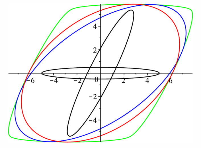
Figure 1 illustrates Theorem 5.5 using the matrices
In the figure, the ellipses are black, the Minkowski sum boundary is green, is blue, and is red.
The area of is approximately 113.14, whereas has area 108.38.
Remark 5.9.
Kurzhanski–Vályi [17] gives a family of inner ellipsoids , with
where is any symmetric positive-definite matrix. The union of the ellipsoids covers the entire Minkowski sum . If or , then .
5.2 Comparison with Brunn-Minkowski
The Brunn-Minkowski inequality states that
(If are both convex and have positive volume, then equality holds if and only if they are homothetic, i.e., .) For ellipsoidal bodies and , the first inequality of (67) gives a sharper inequality than Brunn-Minkowski:
Theorem 5.10.
Proof.
The first two inequalities of the theorem follow from the optimality of John’s ellipsoid and (67). The Minkowski inequality for determinants yields
∎
Consider for example, the case when and , are degenerate ellipses with and . Each has zero area, but the Minkowski sum will be a rectangle. In this case, Brunn-Minkowski gives while Theorem 5.10 gives .
Theorem 5.10 generalizes to the sum of ellipsoids, although the bounds become looser. For example, given three ellipsoids , defined by , , , a lower bound on the Minkowski sum determinant can be obtained recursively by considering the three positive matrices
each defining an inner ellipsoid for . Then
5.3 Upper Bounds for Minkowski Sums of Ellipsoids
| (78) |
for with
| (79) |
By the method of Section 5.1, if and only if
| (80) |
In fact, if for , then by the Cauchy-Schwarz inequality,
Imposing the constraint
and observing that
reproduces the well-known constraint (80), and hence when satisfies (79).
In the case when , the outer ellipsoid defined by (78)–(79) has minimal volume when
| (81) |
where is the (unique) positive solution of the equation
| (82) |
see [15, 17, 24]. Thus, (67) provides the upper bound on the volume
| (83) |
where are given by (81)–(82). When , with being a rotation matrix, symmetry yields and thus .
In some contexts where rapid computations are required, alternative choices can be made with good effect such as
| (84) |
The choice in (84) gives the enclosing ellipsoid that minimizes the sum of squared semi-axes lengths [17, Lemma 2.5.2]. A heuristic choice motivated by (84) for the case of an -fold Minkowski sum is
| (85) |
It can be shown that the minimal volume ellipsoid of the form (78) enclosing an -fold Minkowski sum is defined by [15, 17]
| (86) |
where is the unit vector that minimizes . That is, the optimal choice for is defined by
| (87) |
An algorithm for finding so that defines the minimal volume ellipsoid is given in [15].
6 Bounds on Volume Using Steiner’s Formula
Given a convex body , Steiner’s Formula gives the volume of the offset body as
| (90) |
where the quantities are the quermasssintegrals of . (See [4, 14, 17].) In particular, Steiner’s Formula for the area of the Minkowski sum of a 2D convex body with a disk of radius is
where is the area of , is the length of the boundary (i.e., its perimeter), and
is the integral of curvature around the boundary. Consequently,
Since
Steiner’s formula can be used to compute exactly as
| (91) |
where are the eigenvalues of and is an elliptic integral.
Letting , it is possible to repeat the same procedure as above to compute the exact area as
This is exactly computable using (91) and the general fact that
This approach leads to a recursive algorithm to exactly compute the area of an -fold Minkowski sum of ellipses in the plane.
In higher dimensions, we can take a similar approach to tightly bound the volume of Minkowski sums, but the approach will no longer give an exact equality for ellipsoids. This is now demonstrated in the 3D case.
Steiner’s Formula for the volume of the Minkowski sum of a 3D convex body with a ball of radius is
where is the volume of , is the surface area of the boundary , and and are respectively the integral of mean and Gaussian curvature over the whole boundary . From the Gauss-Bonnet Theorem,
Consequently
Therefore, for the sum of a pair of 3D ellipsoids
the same approach as in the planar case can be used to exactly compute
The quantities in this formula can be computed using (65). In particular, for an ellipsoid ,
Furthermore, by Theorem 1.2,
| (92) |
If it is assumed that and are exactly computable for 3D ellipsoids, then the above provides a closed-form formula for .
Following the same logic as in the planar case,
| (93) |
where is fed forward from the previous step. Moreover, by the additivity of in 3D (see [14, 22], or by (62) and (92)),
but no such equality exists for surface area. Since it is known that is the average area of the orthogonal projections of onto planes in [22], it follows that if then
| (94) |
This can be used together with the ellipsoidal bounds in Section 5 to provide volume bounds in (93). The same reasoning can be applied in higher dimensions using Steiner’s Formula (90), where the result of Theorem 1.2 continues to be applicable.
Acknowledgements
This work was supported by National Science Foundation grants CCF-1640970 and IIS-1619050.
References
- [1] K. M. Ball, Volume ratios and a reverse isoperimetric inequality, J. London Math. Soc. (2) 44 (1991), 351–359.
- [2] K. M. Ball, Ellipsoids of maximal volume in convex bodies, Geom. Dedicata 41 (1992), 241–250.
- [3] R. Bhatia, Positive Definite Matrices, Princeton University Press, 2006.
- [4] Yu. D. Burago and V. A. Zalgaller, Geometric inequalities. Translated from the Russian by A. B. Sosinskiĭ. Grundlehren der Mathematischen Wissenschaften [Fundamental Principles of Mathematical Sciences], 285. Springer Series in Soviet Mathematics. Springer-Verlag, Berlin, 1988.
- [5] F. L. Chernousko, State Estimation for Dynamic Systems, CRC Press, 1994.
- [6] G. S. Chirikjian and B. Shiffman, Collision-free configuration-spaces in macromolecular crystals, Robotica 34 (8), 1679–1704 (2016).
- [7] E. De Giorgi, Su una teoria generale della misura -dimensionale in uno spazio ad dimensioni, Ann. Mat. Pura Appl. 36 (1954), 191–213.
- [8] C. Durieu, E. Walter, and B. Polyak, Multi-Input Multi-Output Ellipsoidal State Bounding, Journal of Optimization Theory and Applications, Vol. 111, No. 2, pp. 273–303, 2001.
- [9] H. Federer, Geometric Measure Theory, Springer-Verlag, Berlin, 1969.
- [10] W. H. Fleming, Early Developments in Geometric Measure Theory, Indiana Univ. Math. J., Vol. 69, No. 1 (2020), 5–36.
- [11] W. J. Firey, The determination of convex bodies from their mean radius of curvature functions. Mathematika 14 (1967), 1–13.
- [12] R. J. Gardner, The Brunn-Minkowski inequality. Bull. Amer. Math. Soc. 39, 355–405, 2002.
- [13] E. L. Grinberg. Isoperimetric inequalities and identities for k-dimensional crosssections of convex bodies. Math. Ann. 291. 75–86, 1991.
- [14] P. M. Gruber, Convex and Discrete Geometry, Springer, 2007.
- [15] A. Halder, On the parameterized computation of minimum volume outer ellipsoid of Minkowski sum of ellipsoids. In 2018 IEEE Conference on Decision and Control (CDC) (pp. 4040–4045). IEEE, 2018.
- [16] F. John, Extremum problems with inequalities as subsidiary conditions. Studies and Essays Presented to R. Courant on his 60th Birthday, January 8, 1948, Interscience Publishers, Inc., New York, N. Y., 1948, pp. 187–204.
- [17] A. B. Kurzhanski and I. Vályi, Ellipsoidal Calculus for Estimation and Control, Systems & Control: Foundations and Applications, Birkhäuser Boston and International Institute for Applied Systems Analysis, 1997.
- [18] A. A. Kurzhanskiy and P. Varaiya, Ellipsoidal Toolbox (ET), 45th IEEE Conference on Decision and Control, pp. 1498–1503, 2006.
- [19] S. Ruan and G. S. Chirikjian, Closed-Form Minkowski Sums of Convex Bodies with Smooth Positively Curved Boundaries, preprint, arxiv.org/abs/2012.15461.
- [20] S. Ruan, K. L. Poblete, Y. Li, Q. Lin, Q. Ma, G. S. Chirikjian, Efficient Exact Collision Detection between Ellipsoids and Superquadrics via Closed-form Minkowski Sums. 2019 International Conference on Robotics and Automation (ICRA), 1765–1771.
- [21] L. A. Santaló, On complete systems of inequalities between elements of a plane convex figure. (Spanish) Math. Notae 17 (1959/61), 82–104.
- [22] R. Schneider, Convex Bodies: The Brunn-Minkowski Theory, 2nd ed. Encyclopedia of Mathematics and Its Applications 151, Cambridge Univ. Press, 2014.
- [23] B. Shiffman, S. Lyu, G. S. Chirikjian, Mathematical aspects of molecular replacement. V. Isolating feasible regions in motion spaces, Acta Cryst. A76, 145–162, 2020.
- [24] O. V. Sholokhov, Minimum-volume ellipsoidal approximation of the sum of two ellipsoids. Cybernetics and Systems Analysis, 47(6), pp. 954–960, 2011.
- [25] G. Stolzenberg, Volumes, limits, and extensions of analytic varieties. Lecture Notes in Mathematics, No. 19, Springer-Verlag, Berlin-New York, 1966.
- [26] H. Whitney, Geometric integration theory. Princeton University Press, Princeton, N. J., 1957.
- [27] Y. Yan and G..S. Chirikjian, Closed-form characterization of the Minkowski sum and difference of two ellipsoids. Geometriae Dedicata, 177(1), pp. 103–128, 2015