Event-Triggered Control for
Mitigating SIS Spreading ProcessesJournal: Annual Reviews in Control
Abstract
In this paper, we investigate the problem of designing event-triggered controllers for containing epidemic processes in complex networks. We focus on a deterministic susceptible-infected-susceptible (SIS) model, which is one of the well-known, fundamental models that capture the epidemic spreading. The event-triggered control is particularly formulated in the context of viral spreading, in which control inputs (e.g., the amount of medical treatments, a level of traffic regulations) for each subpopulation are updated only when the fraction of the infected people in the subpopulation exceeds a prescribed threshold. We analyze the stability of the proposed event-triggered controller and derive a sufficient condition for a prescribed control objective to be achieved. Moreover, we propose a novel emulation-based approach towards the design of the event-triggered controller, and show that the problem of designing the event-triggered controller can be solved in polynomial time using a geometric programming. We illustrate the effectiveness of the proposed approach through numerical simulations using an air transportation network.
Keywords:
Epidemic processes , Event-triggered control , Complex networks , Geometric programmingUTF8mc
1 Introduction
Analysis and control of epidemic processes in complex networks [1] have been studied over the past decades in several research fields including epidemiology, computer science, social science, and control engineering, with applications in epidemic spreading of infectious diseases over human contact networks [2], malware spreading over computer networks [3], rumor propagation [4], and cascading failures or blackouts in electrical networks [5]. This research trend has been further strengthened by the current COVID-19 pandemic, which is posing a significant threat to humanity and economy worldwide. In recent years, an increasing attention has been paid in the systems and control theory toward the analysis and control of epidemic spreading processes, where the amount of medical treatments or a level of traffic regulations are treated as control inputs to be designed, as in [1, 6, 7, 8]. Specifically, control strategies are designed for the mitigation of the epidemic spreading processes (e.g., asymptotic or exponential convergence towards the disease-free state), based on the analysis of network structure and dynamical systems capturing the spreading processes. In this context, most of the early works consider feedforward control strategies, in which suitable control inputs that are applied constantly for all the times will be designed [9, 10, 11, 12]. More recently, dynamical and feedback control strategies have been investigated, in which control inputs are determined to adapt the number of infected people and the time-varying nature of the dynamics [13, 14, 15, 16, 17, 18, 19].
In this paper, we are particularly interested in designing a novel feedback control strategy for a deterministic susceptible-infected-susceptible (SIS) model, which is one of the well-known and fundamental models for the epidemic spreading processes (see, e.g., [20, 21]). The deterministic SIS model can address epidemic spreading processes in the following two different contexts. The first one is the individual-based context, where the model consists of individuals interacting with each other, and the state of each node represents the probability that the individual is infected. The other one is the metapopulation context, where the model consists of subpopulations containing a group of individuals, or called subpopulations, and the state of each node indicates the fraction of the infected individuals in each subpopulation. This paper focuses on the metapopulation context, as the state of each subpopulation can be measured or estimated in real time (see, e.g., [8]), so that the state-feedback controller can be reasonably implemented in practice.
Various dynamical and feedback control strategies for the SIS models have been proposed, see, e.g., [14, 17, 18]. For example, [14] proposed to employ a model predictive control (MPC), in which control inputs are computed by solving a finite horizon optimal control problem online. The authors in [14] also showed that the asymptotic stability of the disease-free state is guaranteed by the proposed controller. Moreover [17] investigated the instability of the disease-free state under a linear state-feedback controller for a bi-virus epidemic spreading model. In addition, [18] proposed a method for designing a time-varying controller for the asymptotic stabilization of the epidemic processes.
Feedback control strategies presented in the aforementioned papers [14, 17, 18] assume that control inputs are updated continuously (for the continuous-time case) or per unit of time (for the discrete-time case). However, such frequent control updates are not necessarily suitable in practice, since a even small fluctuation of the processes forces us to update the control inputs. For example, the level of traffic regulation, which can be regarded as one of the control inputs for mitigating the epidemic spreading processes, is not necessarily realistic to update continuously because even a small adjustment could require enormous efforts. Thus, a more practical approach will be to update the control inputs only when they are necessary, rather than updating the inputs at every time instants. For example, the level of traffic regulation may be preferable to be changed only when the fraction of the infected people in each subpopulation increases or decreases by the prescribed thresholds.
Motivated by the above observation, in this paper we propose to employ an event-triggered control-based framework [22] for containing epidemic spreading processes. In the proposed framework, control inputs for each subpopulation are updated only when the fraction of the infected people in the subpopulation increases or decreases by a given threshold. As can be seen in the current situation of the COVID-19, employing the event-triggered control for the epidemic processes is reasonable and useful in practice, as many countries have been carrying out their mitigation strategies in an event-triggered manner. In Japan, for example, each prefecture has created its own cautionary levels according to the number of COVID-19 cases, in which, for each cautionary level, the contents of requests to prefectural residents are provided (see, e.g., [23]). In other words, each prefecture dynamically updates its own mitigation strategies only when the number of the COVID-19 cases increases or decreases to some extent. Therefore, the event-triggered control-based framework could serve as a useful decision-making system to inform us of when to update our mitigation strategies in response to the dynamic change in the number of infected people in subpopulations.
The main contribution of this paper is to formulate a framework for the event-triggered containment of the deterministic SIS model. We furthermore formulate the event-triggered control in a distributed manner, in which control inputs for each subpopulation (or node in the graph) are updated based on the well-designed local event-triggered conditions. The SIS model may not be appropriate to concretely capture the dynamical behavior for the current COVID-19 pandemic. Nevertheless, this paper can be viewed as a first step towards a rigorous, mathematical formulation of the event-triggered control for mitigating the epidemic spreading. In particular, we provide both theoretical analysis on stability and design procedure of the event-triggered control in a computationally efficient way. Specifically, the technical contribution of this paper is twofold:
- 1.
We derive a sufficient condition for the event-triggered controller to achieve the prescribed control objective. We further show that the condition can be checked by solving a convex program; for details, see Section 4.
- 2.
Based on the analysis given in (i), we then propose a novel framework to design the event-triggered control for mitigating the SIS spreading processes. In particular, we propose to leverage an emulation-based approach (see, e.g., [24, 25]) as a two-step procedure to design parameters of the event-triggered control. As we will see later, the main advantage of employing the emulation-based approach is that the problem of designing the event-triggered control can be formulated by a geometric programming (see, e.g., [26, 27]), which can be translated into the convex program and thus can be solved in polynomial time; for details, see Section 5.
Our approach is related to applications of event-triggered control for multi-agent systems, (see, e.g., [28, 29, 30, 31]). Note that our result differs from these previous results in terms of both analysis and design in the following aspects. While most of the previous works consider linear multi-agent systems with single or double integrator dynamics and the control objective is to asymptotically achieve a consensus, we study the non-linear dynamical system arising from the SIS model and, furthermore, the control objective is not achieving the consensus but to asymptotically suppress the fraction of the infected people below prescribed thresholds. As will be seen in Section 4, this leads to the stability analysis of an event-triggered controller for positive and quadratic dynamical systems, which has not been fully investigated in the literature. The design procedure presented in this paper is the emulation-based design using a geometric programming, which also differs from the ones in the aforementioned works.
The remainder of this paper is organized as follows. In Section 2, we describe dynamics of the SIS model and the control objective to be achieved in this paper. In Section 3, we describe the details of the proposed event-triggered control for the SIS model. In Section 4, we investigate the stability that derives a sufficient condition for achieving the control objective under the event-triggered controller. In Section 5, we provide an emulation-based approach towards the design of the event-triggered controller. In Section 6, numerical simulations are given to illustrate the effectiveness of the proposed approach. Finally, conclusions and future works are given in Section 7.
(Notation and convention): Let , , denote the set of real numbers, positive real numbers, and non-negative integers, respectively. Let denote the vector or matrix whose elements are all . Let and denote the identity matrix and the -dimensional vector whose elements are all . The transpose of vectors and matrices are denoted by . For any real vector , the Euclidean norm and the norm are denoted by and , respectively (i.e., and ). Moreover, let denote the diagonal matrix whose th diagonal equals . In addition, denote by the support of , i.e., we define the set by
For any two real vectors , , we write if and only if for all . Given a set , we denote by the cardinality of .
A directed graph is defined as the pair , where is the set of nodes and is the set of edges. The set of out-neighbors of node is denoted by , i.e., . Similarly, the set of in-neighbors of node (including node itself) is denoted by , i.e., . Note that, from the definition, if a certain node includes the self-loop, both the in- and the out-neighbors include the node itself, i.e., if , then and .
Next, we shall review some basic concepts of the geometric programming [26]. Let the positive variables be given by . A function is called a monomial if it is given of the form: , where and are given constants. Moreover, a function is called a posynomial if it is given of the form: , where and are given constants. Given a set of posynomial functions and a set of monomials , a geometric program is an optimization problem given of the form:
Although a geometric programming is not a convex program by itself, it can be converted into a convex problem with logarithmic changes of variables and logarithmic transformation of the objective and the constraint functions, (see, e.g., [32]). Hence, the geometric program can be solved efficiently in polynomial time.
2 System description and control objective
In this section, we describe the dynamics of the epidemic spreading and the control objective in this paper.
2.1 Deterministic SIS model
As previously stated in the Introduction, we adopt a deterministic susceptible-infected-susceptible (SIS) model in terms of the metapopulation context (see, e,g., [8]). Consider a network that consists of () groups of individuals, which are labeled by . Individuals in each group are affected by those in their own group or those in the neighboring groups. The neighbor relationships among the groups are captured by a directed graph , where is the set of nodes and is the set of edges. If , it means that the node is affected by the node . Since individuals can be affected by those in their own group, the graph has the self-loops at all nodes, i.e., for all . If with , it means that there is a possibility of contact from individuals in node to those in node .
In the (metapopulation) SIS model, each node has a -valued state variable representing the fraction of infected individuals in the node. We let the state of node at time denoted by . Under this notation, the scalar represents the fraction of individuals in node that are not infected, which we call susceptible subpopulation. The dynamics of the state variable of node in the SIS model is then expressed as follows:
| (1) |
where and () are called the recovery and the infection rates, respectively. Note that for all , since every node has the self-loop. As shown in (1), the epidemic spreading in the SIS model is captured by the following two processes: (a) infected individuals in node recover from infection according to the recovery rate , and (b) susceptible individuals in node are infected either from the node itself according to the infection rate or other nodes having their edges to according to the infection rates , .
In this paper, it is supposed that we can dynamically control the recovery and the infection rates (see, e.g., [14]). For example, the recovery rate can be controlled by increasing or decreasing the amount of medical resources and treatments. On the other hand, the infection rates from the neighbors can be controlled by traffic regulations (e.g., decreasing the number of flights) or a closure of facilities such as the sightseeing places. This consideration allows us to replace the constants and in (1) with the time-dependent functions and , respectively, where and () represent the natural (or, baseline) recovery and infection rates before intervention, whereas the time-dependent scalars and () for represent the effect from applying control inputs and are assumed to satisfy and for all . Then, the original SIS dynamics (1) is rewritten as follows:
| (2) |
The model (2) can be further written in a vectorial form as
| (3) |
where is the state vector and the matrices , , , , and are defined by
| (4) | ||||
by using the vectors and .
2.2 Control objective
In this paper, we consider the following control objective: for every initial state , there exists such that the state trajectory satisfies
| (5) |
where is the number of given control objectives, are given vectors, and are given thresholds. Using (5), we can express various control objectives. For example, suppose that we would like to stabilize below the threshold for all in finite time. This control objective can be expressed by (5) with , for all , and () being the th canonical basis of . For another example, suppose that we divide the set of all the nodes into groups, i.e.,
| (6) |
with (for the illustration, see Fig. 1), and we would like to stabilize the average of the states in each group below the threshold in finite time, i.e.,
| (7) |
for some . This control objective can be expressed by (5) if we choose and define by
| (8) |
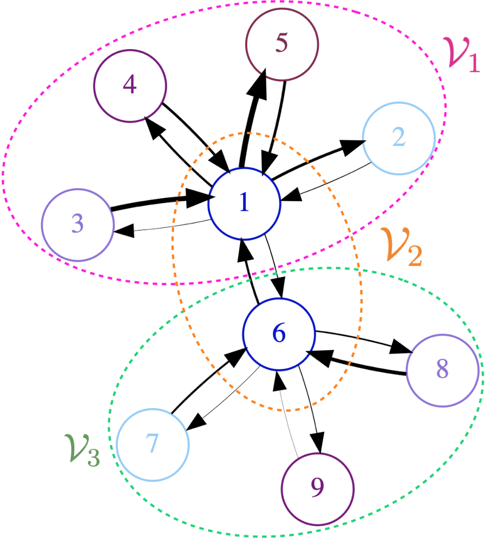
We can confirm that the control objective (5) includes the case of achieving asymptotic stabilization of the origin by setting , for all , and letting () be the th vector in the canonical basis of . Hence, (5) provides the control objective in a more flexible way than the asymptotic stabilization of the origin.
3 Event-triggered control
As previously described in the Introduction, conventional feedback control strategies for the SIS models assume that the control inputs can be updated continuously, i.e., the amount of medical resources and the qualitative degree of traffic regulations must be changed continuously or even per unit of time. However, such frequent control updates are not necessarily suitable in practice, since even a small fluctuation of the states (fraction of infected individuals) forces us to update the control inputs. Hence, a more suitable approach would be to update the control inputs only when they are needed instead of continuously, i.e., the amount of medical resources and the traffic regulations are changed only when the fraction of infected individuals increases or decreases by the prescribed thresholds. This leads us to the usage of an event-triggered control [22], in which the control inputs are updated only when they are needed according to a well-designed event-triggered condition (as detailed below).
To formulate the proposed event-triggered control strategy, let with be the triggering time instants when control inputs for the recovery rate for node , , and the infection rates from node to its out-neighbors (including the node itself), , , are updated. For simplicity, it is assumed that the initial updating time instants for all the nodes, i.e., , , are given. For any , node evaluates the following event-triggering condition
| (9) |
where denotes the error between and the state at the latest triggering time before , i.e.,
| (10) |
where the scalars , , are the parameters to characterize the event-triggered condition. The parameters , , are called the event-triggering gains, which will be designed later in this paper. It is assumed that the event-triggering gains are chosen such that
| (11) |
for all . If the condition (9) is satisfied, then node does not update the control inputs, i.e., . On the other hand, if (9) is violated, then node updates the control inputs, i.e., . More specifically, the triggering time instants are given as follows:
| (12) |
for all .
Our choice of the event-triggering condition in (9) (as well as the triggering time instants in (12)) is motivated as follows. Intuitively, the term in the right hand side of (9) becomes more dominant than when is large, and is more dominant than when is very small. For example, when the state is very small, the control inputs are no more updated unless the error exceeds . In particular, when the state is decreasing and eventually satisfies for all (for some ), the control inputs are no more updated after since the error does not exceed for all . Therefore, by using the event-triggering condition (9), it can be expected that the frequency of the control updates becomes less and less as the state gets smaller and smaller.
Remark 1.
It is necessary for the event-triggering gains to be designed as for all in our problem set-up in order to guarantee that the inter-event times are always positive, i.e., avoid the Zeno behavior or satisfy an event-separation property (see, e.g., [22, 33]). If we set , we cannot guarantee that the inter-event times are always positive due to the effect of the term in (2); for certain values of this term, the inter-event times can eventually become zero in finite time, (see, e.g., [33]). If for all , it follows that, for each , the next triggering time is given at least after the absolute error reaches . Since is continuous for all , there always exists a such that the event-triggered condition (9) is satisfied for all , and so the inter-event times are positive for all the times.
For each node , the control inputs are updated according to the following linear state feedback controller:
| (13) | ||||
| (14) |
for all , where , , , are parameters to characterize the control strategy. The parameters , , , are called the control gains, which will be designed together with the event-triggering gains later in this paper. It is assumed that the control gains must be chosen such that
| (15) |
for all and , where and (, ) are given upper bounds for the control gains of and , respectively.
The following proposition establishes the invariance of the region under the event-triggered controller (13), (14).
Proposition 1.
Proof.
Since we apply the event-triggered controller (13), (14), where the control gains are chosen to satisfy (15) for all and , it follows that the control inputs are piecewise continuous in and satisfy and for all . Let
| (16) |
with being the collection of all the control inputs, i.e., . Moreover, let . Since is bounded and is smooth in , there exists an such that for all , , and , satisfying the Lipschitz condition in [34]. Hence, the solution of exists and unique in . The fact that the state trajectory remains in for all the times can be shown as follows. Let be the boundary of and let for all given by
| (17) | ||||
| (18) |
Note that the union of and for all comprises . In addition, let and for be the outer normal vectors with respect to and , respectively, i.e., (resp. ) is the vector whose -th element is (resp. ) and otherwise. Then, for all , , and , we obtain
| (19) |
In addition, for all , , and , we obtain
| (20) |
(19) and (20) imply that, for every on the boundary of and for every , , and , the vector field is tangential or pointing inwards , which shows that is an invariant set (for the related analysis, see, e.g., [35]). Therefore, if , the state trajectory satisfies for all . ∎
4 Stability Analysis
In this section, we analyze the stability of the closed-loop system for the SIS model (2). In particular, we investigate a sufficient condition that, under appropriate selections of the control and the event-triggering gains, the control objective (5) is achieved by applying the event-triggered controller (13), (14).
We start our stability analysis by introducing several additional parameters and notations. First, we denote the set of control and the event-triggering gains as , , and . We then define the matrices
| (21) | ||||
| (22) |
Second, we define a candidate Lyapunov function by
| (23) |
for a given Lyapunov parameter . Note that we can make use of the candidate Lyapunov function as the linear function of , since the dynamics (2) is non-negative for every (see Proposition 1). Moreover, let for all be given by
| (24) |
where is defined in (5). That is, represents the smallest value among the set of the Lyapunov parameters whose indices belong to the support of . Additionally, define the vectors by
| (25) | ||||
| (26) |
Finally, define the matrix and the set by
| (27) | ||||
| (28) |
where , , and is an any positive constant.
The following theorem gives a sufficient condition for the control objective (5) to be achieved and is the main result of this section.
Theorem 1.
Consider the SIS model (2), the event-triggered controller (13), (14), and the control objective (5). Assume that the control and the event-triggering gains satisfying (11) and (15) are chosen such that the following conditions are satisfied:
| (29) |
for all , where is defined according to the following optimization problem:
| (30) |
where is defined in (28). Then, for any , the control objective (5) is achieved by applying the event-triggered controller (13), (14). In addition, for every selection of the control and the event-triggering gains satisfying (11) and (15), it follows that the optimization problem (30) is strictly convex. ∎
In essence, Theorem 1 states that if the control and the event-triggering gains are appropriately chosen such that (29) is satisfied, then the control objective (5) is achieved by applying the event-triggered controller (13), (14). Theorem 1 also states that the optimization problem (30) is strictly convex for every selection of the control and the event-triggering gains. Hence, the condition (29) can be efficiently checked in polynomial time.
Remark 2.
Proof.
Let us first show that the optimization problem (30) is strictly convex. From (28), the strict convexity of (30) can be shown by guaranteeing that the matrix is positive definite for every selection of the control and the event-triggering gains satisfying (11) and (15). From (27), it can be shown that the -th diagonal element of the matrix , denoted by , is given by
| (31) |
for all . Moreover, the -th () off-diagonal element of the matrix , which is denoted as , is given by
Hence, the difference between the -th diagonal element and the sum of the other elements in the -th row is given by
| (32) |
where we used for all and . Hence, it follows that is a strongly diagonally dominant matrix, which implies that, from the Gershgorin circle theorem [36], the matrix is positive-definite.
Next, we show that the control objective (5) is achieved by applying the event-triggered controller (13), (14). Using (13) and (14), the closed-loop system is given by
| (33) |
Moreover, due to the event-triggered condition (9), it follows that , for all and . Hence, we obtain
| (34) |
Note that for every , we have for all (see Proposition 1). Hence, the last term in (4) can be computed as
| (35) |
Thus, (4) becomes
| (36) |
Using and , we then obtain
| (37) |
By collecting (37) for all , we have
| (38) |
where and . The derivative of the Lyapunov function is then given by
| (39) |
so that .
Now, consider computed from (30). From (30), it follows that for all . Moreover, since (30) is strictly convex and it corresponds to the maximization of the linear function (i.e., ) over the ellipsoidal set (i.e., ), the optimal solution of (30) is unique and lies on the boundary of 1)1) 1) For this clarification, see, e.g., the solution to Exercise 4.21(b) in [26], in which it can be verified that the optimal solution lies on the boundary of the ellipsoidal set .. In other words, we have , where is the optimal solution of in (30) (i.e., ). Therefore,
| (40) |
for all . Hence, by taking the contrapositive of (40), we obtain for all . Therefore, from (39), we obtain
| (41) |
Eq. (41) implies that the derivative of the Lyapunov function along the trajectory of the SIS model satisfies
| (42) |
where . Since is negative in , any state trajectory starting in converges to the set in finite time (see e.g., Section 4.8 in [34]). Moreover, since is negative in , it is shown that is an invariant set, i.e., once the state enters , it remains therein for all future times. Therefore, for every , there exists such that
| (43) |
Moreover, since is defined by (24), we have
| (44) |
which implies that
| (45) |
Hence, if (29) holds for all , we have , for all and . Therefore, for any , the control objective (5) is achieved by applying the event-triggered controller (13), (14). ∎
5 Event-triggered controller synthesis
In this section, we investigate an event-triggered controller design. As shown in Theorem 1, the control objective (5) is achieved if the control and the event-triggering gains satisfy the inequality (29) for all , which we can efficiently check by convex optimization. However, it is not necessarily easy to directly use the inequality (29) for designing the control and the event-triggering gains, because the vector and the matrix used to define the set in the optimization problem (30) contain the parameters to be designed. In order to overcome this difficulty, in this section, we present a tractable and numerically efficient method for designing the control and event-triggering gains via convex relaxation techniques for the conditions required in Theorem 1, such that both the control and the event-triggering gains are designed in polynomial time.
Specifically, we propose an emulation-based approach to the design of the control and the event-triggering gains. The emulation-based approach is the well-known technique to design the event-triggered controller (see, e.g., [22, 24]), and basically it consists of the two steps. First, we find the set of the control gains under the assumption that the continuous-time controller is implemented. Second, using the control gains obtained by the first step, we then design the event-triggering gains, such that the control objective is achieved. As will be shown below, both the former and the latter problems can be formulated by geometric programmings [26], meaning that the control and the event-triggering gains can be found efficiently in polynomial time.
5.1 Designing control gains
We start by designing the control gains , for all and . As mentioned above, in the emulation-based approach, the control gains are designed under the assumption that the continuous-time controller is implemented; that is, (13) and (14) are replaced by
| (46) | ||||
| (47) |
for all . Moreover, define the constants , for all by
| (48) | ||||
| (49) |
From (48), we obtain with . In addition, define the set and the constants for all by
| (50) | ||||
| (51) |
The following proposition shows that the set of the control gains achieving the control objective (5) under the continuous-time controller can be found by solving a geometric programming problem.
Proposition 2.
Consider the SIS model (2), continuous-time controller (46), (47), and the control objective (5). Moreover, let for all , and denote the optimal solution of for all , and , in the following geometric programming:
| (52) | ||||
| (53) | ||||
| (54) | ||||
| (55) | ||||
| (56) |
where is the vector that collects all the decision variables in the optimization problem, i.e., and is a given posynomial function. Then, the control objective is achieved by applying the continuous-time controller, in which the control gains , are given by
| (57) |
for all and . ∎
Proposition 2 is shown by providing sufficient conditions for the control objective to be achieved under the continuous-time controller (see Lemma 1 in Appendix A), and then translate the conditions into the posynomial constraints as shown in (52)–(56). For the detailed proof, see Appendix A.
Remark 3 (On the selection of the cost function ).
For example, one could select the (posynomical) cost function as follows:
| (58) |
where for all are given weights. Note that and for all and are the variables in the optimization problem satisfying and (see Appendix A). Moreover, , for all and are the constants that represent the upper bounds of the control gains (see (15)). Hence, reducing (resp. ) implies to reduce the cost of (resp. ). Therefore, minimizing (58) subject to the constraints (52)-(56) aims at obtaining small control gains while achieving the control objective.
5.2 Designing event-triggering gains
Let us now design the event-triggering gains, i.e., for all . Consider the event-triggered controller (13), (14), in which the triggering time instants are given according to (12). Fix the control gains by , for all , , where , (, ) are the optimal control gains that are designed by solving the geometric programming problem proposed in Proposition 2. Moreover, define the constants for all by
| (59) |
For technical reasons, we make the following assumption:
Assumption 1.
For all , .
Recall that and are defined in (48) and (50), respectively. Hence, Assumption 1 implies that, for all satisfying , the following condition is satisfied:
| (60) |
Hence, (60) implies that the (optimal) control gains , , , should be chosen large enough such that is positive.
Remark 4.
The condition required in Assumption 1 can be indeed satisfied by imposing an additional constraint in the geometric programming presented in Proposition 2. From (60), the control gains , for all and must be chosen such that for all . This leads to the following posynomial constraint:
| (61) |
where is a given arbitrary small positive constant. Hence, is achieved by additionally imposing (61) for all in the geometric programming provided in Proposition 2.
The following proposition shows that the event-triggering gains achieving the control objective can be found by solving the geometric programming problem:
Proposition 3.
Consider the SIS model (2), event-triggered controller (13), (14), and the control objective (5). Let Assumption 1 hold, and let , , , for all and be the optimal solution of , , , for all and , in the following geometric programming:
| (62) | ||||
| (63) | ||||
| (64) | ||||
| (65) | ||||
| (66) | ||||
| (67) |
where is the vector that collects all the decision variables in the optimization problem, i.e., and is a given posynomial function. Then, the control objective is achieved by applying the event-triggered controller (13), (14), in which the event-triggering gains are given by
| (68) | ||||
| (69) |
∎
Proposition 3 is proven by modifying the conditions required in Theorem 1 (see Lemma 2 in Appendix B), so that the conditions required to achieve the control objective can be translated into the posynomial constraints as shown in (62)–(67). For the detailed proof, see Appendix B.
Remark 5 (On the selection of the cost function ).
For example, one could select the cost function as follows:
| (70) |
where for all are given weight parameters. Note that and for all are the variables satisfying (see Appendix B), and that for all are the event-triggering gains. Hence, increasing (resp. ) implies to reduce the cost of (resp. ). From (12), increasing and allow us to reduce the number of the control updates. Therefore, minimizing (70) subject to the constraints (62)–(67) implies to obtain large event-triggering gains so as to reduce the number of the control updates while achieving the control objective.
6 Some discussions on the proposed approach
In this section, we provide some discussions on the proposed approach. In Section 6.1, we provide a way of how to design the Lyapunov parameter . In Section 6.2, we discuss a conservativeness of the geometric programming problems in Proposition 2 and 3 with respect to the condition derived in Theorem 1.
6.1 On designing the Lyapunov parameter
Note that the Lyapunov parameter should be given in Proposition 2 (and Proposition 3), which means that must be chosen apriori before designing the control and the event-triggering gains. For example, one could choose by solving the following linear program:
| (71) |
where is a given positive constant. Since for all (see (48)), the optimization problem (71) aims at finding such that is minimized. Moreover, recall that the vector has been utilized in the derivative of the Lyapunov function under the continuous time controller:
| (72) |
(see (88) in the Appendix). Hence, intuitively, if we have smaller components of , , then the term becomes smaller and so we can obtain a larger domain of for which is ensured to be negative: . Thus, designing such that becomes small may have the potential to enlarge the domain of attraction. Note that it is indeed difficult to take the matrix into account for designing , since must satisfy the constraint involving the control gains (on the other hand, does not depend on the control gains). In (71), the linear constraint has been utilized to normalize the Lyapunov parameter, so that the sum of all the components of equals . In essence, this avoids the case where the optimal solution of becomes extremely close to zero. For example, if for all , then the cost in (71) is positive for all . Hence, if were not given, we could then obtain the optimal solution as , since it tries to make the cost in (71) as close as possible to , i.e., as .
One might wonder how to select in (71). Here, without loss of generality, we can set ; how we select does not affect the domain of the control gains (resp. the event-triggering gains , ) for which the geometric programming problem in Proposition 2 (resp. Proposition 3) is feasible. Specifically, we have the following result:
Proposition 4.
Let and denote the optimal solution of (71) with and , respectively, where with are any positive constants. Let (P.1) and (P.2) (resp. (Q.1) and (Q.2)) denote the geometric programming problem in Proposition 2 (resp. Proposition 3) with the Lyapunov parameter being given by and , respectively. Then, it follows that the feasibility of (P.1) (resp. (Q.1)) implies the feasibility of (P.2) (resp. (Q.2)), and vice versa.
Proposition 4 implies that the domain of the control gains (resp. event-triggering gains) for which the geometric programming problem in Proposition 2 (resp. Proposition 3) with is feasible equals the one with . Hence, if the cost function of the geometric programming problem in Proposition 2 depends only on the control gains, i.e., , then the optimal solution with equals the one with . In general, we define the cost functions depending only on the control gains, since we would like to optimize these parameters (see (58) as an example of the cost function). Similarly, if the cost function of the geometric programming problem in Proposition 3 depends only on the event-triggering gains, i.e., , then the optimal solution with equals the one with (see (70) as an example of the cost function). For the proof of Proposition 4, see Appendix C.
6.2 On the conservativeness of Proposition 2 and 3
In this section, we discuss the potential conservativeness of Proposition 2 and 3. Note that the posynomial constraints in Proposition 2 and 3 are given as the sufficient conditions to those in Theorem 1. Hence, it is worth discussing how the posynomical constraints derived in Proposition 2 and 3 are conservative with respect to those in Theorem 1. For deriving the posynomial constraints of the control gains (Proposition 2), the sufficiency has arisen since the term in the right hand side of (A) has been replaced by in (98), using the inequalities for all . This conservative operation (i.e., from (A) to (98)) has been taken for all . Thus, the conservativeness for designing the control gains from Proposition 2 increases as the number of the nodes satisfying (i.e., the cardinality of ) increases. In other words, the conservativeness decreases as the number of the nodes satisfying (i.e., the cardinality of ) increases. Recall that is defined as , where (see (50)). Hence, implies
| (73) |
If (i.e., the baseline infection rate for the node itself is larger than the natural recovery rate), then (73) holds. Hence, as the number of nodes satisfying increases, which may be the case where a huge outbreak (i.e., the infection rates are large) happens, the conservativeness for designing the control gains from Proposition 2 decreases.
For deriving the posynomial constraints of the event-triggering gains (Proposition 3), the sufficiency has arisen in (B), since we have used the following inequality: , where (see (27)). The term is the matrix that enumerates the coefficiencies of the cross term in the derivative of (see (37)). Since we neglect this term for deriving the posynomial constraints, it implies that will be more conservatively selected as the number of the in-neighbor nodes for node is larger. In other words, if the number of the in-neighbor nodes for node is very large, very small could be obtained, which could result in frequent control updates (or the geometric programming problem in Proposition 3 may become infeasible).
If the geometric programming problem of finding the control gains (Proposition 2) is not feasible, we have no choice but could try to change the candidate Lyapunov function (i.e., modify the parameter ), or, if allows, try to enlarge the upper bound of the control gains in (15) so as to increase the feasibility domain of the geometric programming problem in Proposition 2. If Proposition 2 is feasible but Proposition 3 is not feasible, we could modify the cost function in Proposition 2 (e.g., change the weight parameters of (58)), or, slightly tighten the constraints in Proposition 2 so as to make Proposition 3 feasible. More specifically, in Proposition 2, we replace the constraints (52), (55), (56) with
| (74) | ||||
| (75) | ||||
| (76) |
where are given positive constants. Note that setting in (74), (75) and (76) corresponds to (52), (55) and (56), respectively. Let for all , and denote an any feasible solution to the posynomial constraints (53), (54), (74)–(76). The corresponding control gains are denoted as . Then, it follows that
| (77) |
Moreover, if , it follows that
| (78) |
Additionally, from (55) and (56), it follows that
| (79) | ||||
| (80) |
Now, consider the feasibility problem provided in Proposition 3: find , , , for all and such that (62)–(67) hold. Suppose that is chosen small enough such that for all . Then, (77), (78), (79) and (80) imply that the posynomical constraints (62)–(67) are all feasible with
| (81) | ||||
| (82) |
Therefore, if we utilize the slightly tightened constraints in Proposition 2, and if it is feasible, we can guarantee the feasibility of the posynomical constraints in Proposition 3.
Even though Proposition 3 becomes feasible, it is still possible that, due to the conservativeness as described above, very small event-triggering gains might be obtained. In such case, we could make use of the result of Theorem 1 in order to reduce the conservativeness. That is, if the resulting according to Proposition 3 are very small for some , we could try to increase these parameters (i.e., for some and the other parameters are fixed) and then check if (29) in Theorem 1 holds. If (29) holds, then it follows that the control objective is achieved even with the modified event-triggering gains. Since the condition in Theorem 1 is less conservative than those in Proposition 3, we have the potential to enlarge the event-triggering gains. Note that (29) can be checked via convex program, since all the control and the event-triggering gains are here given. While the above approach may be somewhat heuristic, it will be useful in practice for reducing the conservativeness of Proposition 3.
7 Numerical simulations
In this section, we demonstrate the performance of the proposed event-triggered controller through a numerical simulation. The simulation have been conducted on MacOS Big Sur, 8-core Intel Core i9 2.4GHz, 32GB RAM using Python 3. Moreover, we used CVXPY for solving convex optimization problems. The code is available on Github: https://github.com/yugaro/etc-sis-solver.
(Problem setup): We apply the proposed approach against the epidemic spreading propagated over an air transportation network consisting of 50 airports in the United States (U.S.). The graph is constructed from the statistical data [37, 38] of the number of passengers and flights. More specifically, we extract the data from [37] the top 50 U.S. airports according to the number of passengers in 2019, and from [38] the number of the flights among the airports. The resulting graph consists of 50 nodes (i.e., ) that represent the set of 50 airports, and the set of edges among different nodes that represent the existence of the directed flights among them. Fig. 2 depicts the resulting graph structure, where the nodes in the network are divided into three groups denoted by , , , which are called Group 1, 2 and 3, respectively.

In this numerical simulation, we randomly choose the baseline recovery rate of each node from a uniform distribution on the interval . On the other hand, each baseline infection rate from the neighbor (, ) is chosen on the interval in accordance with the data [38]. More specifically, each (, ) is chosen to be proportional to the number of the direct flights from the airport corresponding to node to the one corresponding to node , and is normalized such that the maximum value of (, ) equals . Moreover, each baseline infection rate for the node itself , is chosen to be proportional to the population of the city that contains the airport corresponding to the node , and is normalized such that the maximum value of () equals to .
The control objective in this numerical simulation is to achieve (7) for all with , . In other words, we aim at containing the average of the fraction of the infected people in Group 1, 2, and 3 within the corresponding thresholds , and , respectively. As described in Section 2.2, such control objective can be expressed by (5) with appropriate selection of the parameters and for each .
The upper bounds of the control gains are given by , for all and . The Lyapunov parameter in (23) is chosen by solving (71). When solving the geometric programming problem to find the optimal control gains from Proposition 2, we define the cost function by (58) with for all . In addition, when solving the geometric programming problem to find the optimal event-triggering gains from Proposition 3, we define the cost function by (70) with for all .
(Simulation results): Fig. 3(a) plots the state trajectories for all the nodes by applying the event-triggered controller designed by the emulation-based approach proposed in Section 5, where the initial state is randomly given from a uniform distribution on the interval set . For comparisons, we illustrate in Fig. 3(b) the state trajectories without control inputs (i.e., the state trajectories with , for all , , and ), where the initial state is the same as the event-triggered controller. Fig. 3(a) shows that the fraction of infected people are contained effectively by applying the proposed event-triggered controller compared with the control-free case in Fig. 3(b). To verify that the control objective is achieved, we illustrate in Fig. 4 the trajectories of for all under the proposed event-triggered controller (red solid line), without control inputs (green dotted line), the continuous-time controller (46), (47) (see Section 5.1; blue dashed line) whose control gains are the same as the event-triggered controller. Fig. 4 shows that, by applying the event-triggered controller, the average of the fraction of infected people in each group can be appropriately contained such that the control objective is achieved (i.e., converge below the prescribed thresholds , and ), while at the same time preserving almost the same convergence performance as the continuous-time controller. It can be also seen that the event-triggered controller provides a better control performance than the continuous-time controller. To describe why this has happened, recall that the event-triggered controller updates the control inputs only when they are needed, while the continuous controller updates them continuously. Moreover, the linear state-feedback controller is employed under both the continuous controller and the event-triggered controller (see (13), (14)). Thus, when the state (the fraction of the infected people) is decreasing, the control input under the continuous controller is decreasing for all times, while the control input under the event-triggered controller is kept constant during the inter-event times and it decreases only for the update times. Therefore, if the inter-event times are relatively long, the control input under the event-triggered controller tend to be larger than the one under the continuous-time controller. Therefore, the event-triggered controller tends to mitigate the infection further than the continuous-time controller (since it tends to utilize larger control inputs) and thus provides a better performance. Note that, when the state is increasing, the reverse holds; the control inputs under the event-triggered controller tends to be smaller than the continuous-time controller and thus provide worse performance. In this numerical simulation, the event-triggered controller provides a better performance than the continuous time controller, since, as shown in Fig. 3, many states are decreasing for most of the times.
In Fig. 5(a) and (b), we plot the trajectories of the control inputs , for under the proposed event-triggered controller. In addition, Fig. 5(c) illustrates the corresponding inter-event times, i.e., for and . From the figures, we can observe that the control inputs are not updated continuously but are updated aperiodically based on the proposed event-triggered controller. We can furthermore observe the inter-event times tend to be larger as time evolves and the state trajectories converge, which implies that the control inputs are updated only when the fraction of the infected people in each node increases or decreases by the threshold designed by the proposed approach. In summary, we can confirm the validity of the proposed event-triggered controller by showing that, the control inputs for each node are updated only when they are needed while preserving almost the same convergence performance as the continuous-time controller.
8 Conclusions and future works
In this paper, we proposed an event-triggered control-based framework for a deterministic SIS model. In the proposed framework, control inputs for each subpopulation are updated only when the fraction of the infected people increases or decreases by a prescribed threshold, aiming at reducing unnecessarily burden of updating the control inputs. First, we analyzed the stability of the closed-loop system under the event-triggered controller. We in particular derived a sufficient condition for the event-triggered controller to achieve a prescribed control objective. We further showed that the derived conditions are characterized by convex programs, which can be thus efficiently solved in polynomial time. Then, we proposed an emulation-based approach towards the design of the event-triggered controller. We in particular showed that the problem of designing the control and the event-triggering gains can be solved by the geometric programmings, which can reduce to convex programs and can be efficiently solved in polynomial time. Finally, we confirmed the validity of our proposed approach through numerical simulations of an epidemic spreading using an air transportation network.
The following aspects should be further pursued in our future works of research:
- 1.
In the event-triggered control framework presented in this paper, the state for each node needs to be monitored continuously so as to determine the triggering time instants. Moreover, the inter-event times might still be very small especially when a huge outbreak happens. Hence, it is of great importance to provide some constraints on the lower bound of the inter-event times, so as to further reduce the frequency of the control inputs. These issues could indeed be solved by employing the periodic event-triggered control [24], in which the states are measured only periodically (not continuously as in the standard event-triggered control presented in this paper). Therefore, future work involves solving the above issues by formulating the periodic event-triggered control for mitigating the epidemic spreading.
- 2.
In our current problem setup, we impose the constraints on the control gains (see (15)) in order to restrict the amount of the control inputs. However, in this formulation, the upper bound of the control input is utilized only when the state is (i.e., iff ). Hence, it might be more reasonable and realistic to impose the constraints directly on the control inputs, e.g., , for all rather than impose the constraints on the control gains. Hence, considering how to impose , when designing the event-triggered controller for the epidemic spreading should be pursued in our future work.
- 3.
In addition to the above, there exist several research directions that should be further pursued in relation to the current COVID-19 pandemic. For example, it is of both theoretical and practical interest to investigate the event-triggered control of more realistic epidemic models, such as the SIR models, the SEIR models, and various others (see, e.g., [39, 40, 41, 42]). Another important research direction is to develop a theoretical framework for the event-triggered control of epidemics over temporal networks [43, 44] in order to account the intrinsic time-variability of contact networks in the human society. Additionally, time delays arising in the feedback loop as well as parameter uncertainties in the epidemic models (see, e.g., [40]) should be taken into account for further investigations in designing the event-triggered controller.
Acknowledgement
This work was supported in part by JSPS KAKENHI Grant 21H01353 and in part by JST ERATO HASUO Metamathematics for Systems Design Project (No. JPMJER1603).
References
- [1] R. Pastor-Satorras, C. Castellano, P. Van Mieghem, A. Vespignani, Epidemic processes in complex networks, Reviews on Modern Physics 87 (2015) 925–979.
- [2] P. Van Mieghem, J. Omic, R. Kooij, Virus spread in networks, IEEE/ACM Transactions on Networking 17 (1) (2009) 1–14.
- [3] M. Garetto, W. Gong, D. Towsley, Modeling malware spreading dynamics, in: Proceedins of the Twenty-second Annual Joint Conference of the IEEE Computer and Communications Societies, 2003, pp. 1869–1879.
- [4] K. Lerman, R. Ghosh, Information contagion: an empirical study of spread of news on digg and twitter social networks, in: Proceedings of 4th International Conference on Weblogs and Social Media (ICWSM), 2010.
- [5] S. Soltan, D. Mazauric, G. Zussman, Cascading failures in power grids: Analysis and algorithms, in: Proceedings of the 5th International Conference on Future Energy Systems, 2014, p. 195–206.
- [6] V. M. Preciado, M. Zargham, Traffic optimization to control epidemic outbreaks in metapopulation models, in: 2013 IEEE Global Conference on Signal and Information Processing, 2013, pp. 847–850.
- [7] V. M. Preciado, M. Zargham, D. Sun, Traffic control for network protection against spreading processes, in: Proceedings of the 48th Annual Conference on Information Sciences and Systems, 2014, pp. 1–8.
- [8] C. Nowzari, V. M. Preciado, G. J. Pappas, Analysis and control of epidemics: A survey of spreading processes on complex networks, IEEE Control Systems Magazine 36 (1) (2016) 26–46.
- [9] V. M. Preciado, M. Zargham, C. Enyioha, A. Jadbabaie, G. J. Pappas, Optimal resource allocation for network protection against spreading processes, IEEE Transactions on Control of Network Systems 1 (1) (2014) 99–108.
- [10] S. Han, V. M. Preciado, C. Nowzari, G. J. Pappas, Data-driven network resource allocation for controlling spreading processes, IEEE Transactions on Network Science and Engineering 2 (4) (2015) 127–138.
- [11] C. Nowzari, V. M. Preciado, G. J. Pappas, Optimal resource allocation for control of networked epidemic models, IEEE Transactions on Control of Network Systems 4 (2) (2017) 159–169.
- [12] V. S. Mai, A. Battou, K. Mills, Distributed algorithm for suppressing epidemic spread in networks, IEEE Control Systems Letters 2 (3) (2018) 555–560.
- [13] M. Ogura, V. M. Preciado, Epidemic processes over adaptive state-dependent networks, Phys. Rev. E 93 (2016).
- [14] J. Köhler, C. Enyioha, F. Allgöwer, Dynamic resource allocation to control epidemic outbreaks a model predictive control approach, in: 2018 Annual American Control Conference, 2018, pp. 1546–1551.
- [15] L. A. Alarcón-Ramos, R. B. Jaquez, A. Schaum, Output-feedback control of virus spreading in complex networks with quarantine, Frontiers in Applied Mathematics and Statistics 4 (2018) 1–8.
- [16] N. J. Watkins, C. Nowzari, G. J. Pappas, Robust economic model predictive control of continuous-time epidemic processes, IEEE Transactions on Automatic Control 65 (3) (2020) 1116–1131.
- [17] J. Liu, P. E. Paré, A. Nedić, C. Y. Tang, C. L. Beck, T. Başar, Analysis and control of a continuous-time bi-virus model, IEEE Transactions on Automatic Control 64 (12) (2019) 4891–4906.
- [18] S. Gracy, P. E. Pare, H. Sandberg, K. H. Johansson, Analysis and distributed control of periodic epidemic processes, IEEE Transactions on Control of Network Systems (2020).
- [19] A. Janson, S. Gracy, P. E.Paré, H. Sandberg, K. H.Johansson, Networked multi-virus spread with a shared resource: Analysis and mitigation strategies, In arxiv: available at https://arxiv.org/abs/2011.07569.
- [20] L. J. Allen, Some discrete-time si, sir, and sis epidemic models, Math Bioscience 124 (1) (1994) 83–105.
- [21] W. Mei, S. Mohagheghi, S. Zampieri, F. Bullo, On the dynamics of deterministic epidemic propagation over networks, Annual Reviews in Control 44 (2017) 116–128.
- [22] W. P. M. H. Heemels, K. H. Johansson, P. Tabuada, An introduction to event-triggered and self-triggered control, in: Proceedings of the 51st IEEE Conference on Decision and Control, 2012, pp. 3270–3285.
- [23] Causality levels in Akita Prefecture, Japan: https://www.pref.akita.lg.jp/pages/archive/51612#English.
- [24] W. P. M. H. Heemels, M. C. F. Donkers, Model-based periodic event-triggered control for linear systems, Automatica 49 (3) (2013) 698–711.
- [25] W. P. M. H. Heemels, M. C. F. Donkers, A. R. Teel, Periodic event-triggered control for linear systems, IEEE Transactions on Automatic Control 58 (4) (2013) 847–861.
- [26] S. Boyd, L. Vandenberghe, Convex Optimization, Cambridge University Press, 2004.
- [27] M. Ogura, M. Kishida, J. Lam, Geometric programming for optimal positive linear systems, IEEE Transactions on Automatic Control 65 (11) (2020) 4648–4663.
- [28] D. V. Dimagoronas, E. Frazzoli, K. H. Johansson, Distributed event-triggered control for multi-agent systems, IEEE Transactions on Automatic Control 57 (5) (2012) 1291–1297.
- [29] G. S. Seyboth, D. V. Dimagoronas, K. H. Johansson, Event-based broadcasting for multi-agent average consensus, Automatica 49 (1) (2013) 245–252.
- [30] Y. Fan, G. Feng, Y. Wang, C. Song, Distributed event-triggered control of multi-agent systems with combinational measurements, Automatica 49 (2) (2013) 671 – 675.
- [31] C. Nowzari, E. Garcia, J. Cortés, Event-triggered communication and control of networked systems for multi-agent consensus, Automatica 105 (2019) 1 – 27.
- [32] S. Boyd, S.-J. Kim, L. Vandenberghe, A. Hassibi, A tutorial on geometric programming, Optimization and engineering 8 (1) (2007) 67.
- [33] D. P. Borgers, W. P. M. H. Heemels, Event-separation properties of event-triggered control systems, IEEE Transactions on Automatic Control 59 (10) (2014) 2644–2656.
- [34] H. K. Khalil, Nonlinear Systems -third edition-, Prentice Hall, 2002.
- [35] A. Lajmanovich, J. A. Yorke, A deterministic model for gonorrhea in a nonhomogeneous population, Mathematical Biosciences 28 (3) (1976) 221 – 236.
- [36] R. A. Horn, C. R. Johnson, Matrix analysis, Cambridge university press, 2012.
- [37] Federal Aviation Administration (Airport Planning & Capacity Airports): https://www.faa.gov/airports/planning_capacity.
- [38] Airport, airline and route data: https://openflights.org/data.html.
- [39] J. Wang, J. Wang, M. Liu, Y. Li, Global stability analysis of an sir epidemic model with demographics and time delay on networks, Physica A 410 (2014) 268–275.
- [40] F. Casella, Can the COVID-19 Epidemic Be Controlled on the Basis of Daily Test Reports?, IEEE Control Systems Letters 5 (3) (2021) 1079–1084.
- [41] F. Darabi Sahneh, C. Scoglio, P. Van Mieghem, Generalized epidemic mean-field model for spreading processes over multilayer complex networks, IEEE/ACM Transactions on Networking 21 (5) (2013) 1609–1620.
- [42] G. Giordano, F. Blanchini, R. Bruno, P. Colaneri, A. Di Filippo, A. Di Matteo, M. Colaneri, Modelling the COVID-19 epidemic and implementation of population-wide interventions in Italy, Nature Medicine 26 (6) (2020) 855–860.
- [43] M. Ogura, V. M. Preciado, Stability of spreading processes over time-varying large-scale networks, IEEE Transactions on Network Science and Engineering 3 (1) (2016) 44–57.
- [44] P. E. Paré, C. L. Beck, A. Nedić, Epidemic processes over time-varying networks, IEEE Transactions on Control of Network Systems 5 (3) (2017) 1322–1334.
Appendix A Proof of Proposition 2
To prove Proposition 2, let us first provide the following lemma, which gives a sufficient condition for the control objective (5) to be achieved under the continuous-time controller.
Lemma 1.
Consider the SIS model (2), the continuous-time controller (46), (47), and the control objective (5). Assume that the control gains satisfying (15) are chosen such that the following conditions are satisfied:
| (83) |
for all , where is defined according to the following optimization problem:
| (84) |
where with , and is chosen such that the following inequality is satisfied:
| (85) |
Then, for any , the control objective (5) is achieved by applying the continuous-time controller.
(Proof of Lemma 1): The proof is given based on Theorem 1. Applying the continuous-time controller (46), (47) is equivalent to setting the event-triggering gains as and for all (i.e., and ). Hence, by setting in (38), the upper bound of under the continuous-time controller is computed as
| (86) |
The derivative of the Lyapunov function (under the continuous-time controller) is then given by
| (87) | ||||
| (88) |
where we used (see the statement after (48)) and (85) to obtain (88).
Now, similarly to (40), it follows that for all . Hence, by taking the contrapositive, we obtain
| (89) |
Thus, by following the same procedure as (43)–(45), we can show that there exists such that for all and . Therefore, if (83) holds for all , the control objective (5) is achieved by applying the continuous-time controller (46), (47).
We now prove Proposition 2.
(Proof of Proposition 2): From Lemma 1, it is shown that the control objective (5) is achieved by finding control gains , , and a vector , such that the following conditions are all satisfied: (15) for all and , (83) for all and (85). Thus, the decision variables in the design problem here are: , , and . Moreover, the constraints are: (15) for all , , (83) for all and (85). In what follows, we translate the conditions (15), (83), and (85) into the posynomial constraints, so that the control gains can be designed by solving a geometric programming problem. First, the constraint for the -th element of (i.e., ) in (85) is given by
| (90) |
Summing in both sides of (90), we obtain
| (91) |
where is the constant defined in (49). Define the new decision variables , for all by
| (92) |
Then, the constraint (91) results in (52), which is the posynomial constraint (with respect to the variables , , ). With the new decision variables , (), the constraint (15) is then rewritten as and for all . This leads to (53), (54), which are the posynomial constraints. Let us now translate (83) into the posynomial constraint. First, observe that
| (93) |
where
| (94) |
Hence, we obtain
| (95) |
where and . Thus, the optimization problem (84) can be analytically solved as:
| (96) |
Therefore, the constraint (83) is given by
| (97) |
where the set is defined in (50). Note that (A) is not yet a posynomial constraint, since the term in the right hand side involves the variable . In order to convert (A) into the posynomial constraint, notice that, from (91), we have for all . Hence, we obtain for all . Thus, a sufficient condition to satisfy (A) is given by
| (98) |
for all . Define a new variable , such that the following constraint is satisfied:
| (99) |
Thus, we have
| (100) |
Appendix B Proof of Proposition 3
Before proving Proposition 3, let us show that the following lemma holds as a slight modification of Theorem 1:
Lemma 2.
Consider the SIS model (2), the event-triggered controller (13), (14), and the control objective (5). Assume that the control and the event-triggering gains satisfying (11) and (15) are chosen such that the following conditions are satisfied:
| (101) |
for all , where is defined according to the following optimization problem:
| (102) |
where with , , and the vectors are defined such that the following inequalities satisfied:
| (103) | ||||
| (104) |
Then, for any , the control objective (5) is achieved by applying the event-triggered controller.
As shown in the proof below, Lemma 2 is a more conservative result than Theorem 1, in the sense that it provides sufficient conditions to the ones provided in Theorem 1. However, Lemma 2 is useful for translating the conditions required to achieve the control objective into the posynomial constraints (see the proof of Proposition 3 below).
(Proof of Lemma 2): From Theorem 1, it is shown that the control objective (5) is achieved by finding the the control and the event-triggering gains, such that (29) is satisfied for all . From (25), (26), and (27), it follows that
| (105) |
where we used (103) and (104) to obtain (B). Hence, it follows that for all . Therefore, letting , we have (recall that is defined in (28)). Hence, in (30) satisfies
| (106) |
Thus, for all implies for all . Therefore, if the control and the event-triggering gains are chosen such that (102) is satisfied for all , the control objective (5) is achieved by applying the event-triggered controller.
Let us now prove Proposition 3.
(Proof of Proposition 3): Fix the control gains by , for all and . From Lemma 2, it is shown that the control objective (5) is achieved by finding event-triggering gains , , and vectors , , such that the following conditions are all satisfied: (11) for all , (101) for all , (103) and (104). Thus, the decision variables in the design problem here are: , for all , and . Moreover, the constraints are: (11) for all , (101) for all , (103) and (104). In what follows, we translate the conditions (11), (101), (103), and (104) into the posynomial constraints, so that the event-triggering gains can be designed by solving a geometric programming problem. First, the constraint for the -th element of (i.e., ) in (103) is given by
| (107) |
where is the constant defined in (59). Thus, defining the new variables by for all , we obtain the following constraint:
| (108) |
which yields the posynomial constraint (62). Moreover, the constraint for the -th element of (i.e., ) in (104) is given by
| (109) |
where is the constant defined in (48). If , we have and so . This implies that (109) is the posynomial constraint. Thus, we obtain for all , which yields the posynomial constraint (62). If , we have , since (see (69)). Note that we have from Assumption 1. Thus, the constraint (109) for all is trivially given by , .
Using the new decision variable , the constraint of (i.e., ) is rewritten as . This leads to the posynomial constraint (64). The constraint for is given by (66), which follows trivially.
Let us now translate (101) into a posynomial constraint. As with (96), the optimization (102) is analytically solved as
Appendix C Proof of Proposition 4
Let and denote the solution to (71) with and , respectively, where are any positive constants. From (71), it can be easily shown that , where . Here, we will only prove for the geometric program in Proposition 2 (i.e., the feasibility of the geometric program in Proposition 2 with implies the one with and vice versa), since the proof for Proposition 3 is given in the same way with Proposition 2. Let for all , and be an any feasible solution that satisfies the posynomial constraints in Proposition 2 with . In other words, we have
| (114) | ||||
| (115) | ||||
| (116) | ||||
| (117) | ||||
| (118) |
where
| (119) |
with . Multiplying in both sides of (114), we obtain
Letting , we obtain
| (120) |
where we used . Moreover, by multiplying in both sides of (117), it follows that
Letting with , we obtain
| (121) |
where we used . In addition, by multiplying in both sides of (118) in the above, we obtain
| (122) |
Now, consider the feasibility problem of the posynomial constraints with : find for all , and such that
(120), (121), (122) imply that the above problem is feasible with
| (123) | ||||
| (124) |
Thus, the feasibility of the geometric program in Proposition 2 with implies the feasibility of the geometric program in Proposition 2 with . It can be shown in the same way that the feasibility of geometric program with implies the feasibility of the geometric program with .