Phase Transitions in Frequency Agile Radar Using Compressed Sensing

We introduce the signal model of FAR following [12] and [13]. We start with the expressions of the transmissions and the received echoes from a single scattering point, representing target or clutter. We then extend the echo model to the case of multiple targets/clutter.

A FAR system changes the frequencies from pulse to pulse. Suppose that the radar transmits $N$ monotone pulses during a coherent processing interval (CPI). The carrier frequency of the $n$-th pulse can be written as $f_{n}=f_{c}+C_{n}\Delta f$, where $f_{c}$ represents the initial frequency, $\Delta f$ represents the frequency step, and $C_{n}$ is the $n$-th random modulation code. We assume that all the modulation codes are independently and identically distributed (i.i.d.) random variables with uniform density on $\mathcal{M}:=\{0,1,\ldots,M-1\}$, i.e., $C_{n}\sim U(\mathcal{M})$. Then the $n$-th transmitted pulse, $n\in\mathcal{N}:=\{0,1,\ldots,N-1\}$, is written as

where $T_{r}$ is the pulse repetition interval (PRI), $T_{p}$ is the pulse duration, and ${\rm rect}(t)$ equals 1 when $0\leq t\leq 1$ and 0 otherwise.

The received echoes can be seen as delays of transmissions. To clearly present the signal model, we assume that there exists only one ideal scatterer with complex scattering coefficient $\zeta$, which has an initial range $r$ from the radar and is moving along the radar’s line of sight at a fixed speed of $v$. The time delay between the received and the transmitted signal at time instant $t$ takes the form $\tau(t)\coloneqq\frac{2(r+vt)}{c}$, where $c$ is the velocity of light. Under the stop-and-hop assumption [26], it holds that $\tau(t)\approx\tau(nT_{r})$ during the $n$-th pulse. Thus, the received echo of the $n$-th transmission can be expressed as

After down-conversion, the received echoes become

Substituting (2) and (1) into (3) and rearranging, we obtain

where $\epsilon_{n}\coloneqq 1+\frac{C_{n}\Delta f}{f_{c}}$. The parameters $\ddot{\zeta}:=\zeta e^{-j4\pi f_{c}r/c}$, $f_{r}\coloneqq-\frac{2\Delta fr}{c}$ and $f_{v}\coloneqq-\frac{2f_{c}vT_{r}}{c}$, representing the effective intensity, range frequency and velocity frequency, respectively, are unknown and need to be estimated.

The down-converted echoes are sampled at the Nyquist rate of a single pulse, $f_{s}=\frac{1}{T_{p}}$, at time instances, $t=nT_{r}+\frac{l_{s}}{f_{s}}$, $l_{s}=0,1,\ldots,\left\lfloor T_{r}f_{s}\right\rfloor$. Each sample corresponds to a crr (crr) bin. The coarse range will be refined by estimating $f_{r}$ or $r$ from the echoes. Here, $f_{r}$ and $r$ are referred as the hrr information. Since data from those bins are processed identically and individually, without loss of generality, we assume that the target is located in the $l_{s}$-th CRR bin, and that the target does not move outside the bin during the CPI. Consequently, the ${\rm rect}(\cdot)$ term in (4) at the $l_{s}$ sampling instance equals 1, so that sampled $S_{D}(n,t)$ becomes

The model (5), derived for the case of a single scatterer, can be extended to the setting in which $K$ targets/clutter exist in a CRR bin. Particularly, we denote by $v_{k}$ and $f_{v_{k}}$ the velocity and velocity frequency of the $k$-th target (or clutter unit), respectively, with $k=0,1,\ldots,K-1$, and assume that the $k$-th target is composed of $Q_{k}$ scatterers, moving at the same speed while the ranges and scattering intensities are different. For the $i$-th scatterer of the $k$-th target, ${\ddot{\zeta}}_{ki}$, $r_{ki}$ and $f_{r_{ki}}$ denote the scattering coefficient, initial range and range frequency, respectively. We then extend (5) into a model for multiple targets as follows,

Here, $\{\ddot{\zeta}_{ki},f_{r_{ki}},f_{v_{k}}\}$ are unknown and need to be estimated from $S_{S}(n)$.

In the next subsection, we arrange the signal model in matrix form, which suggests a block sparse recovery approach for range-Doppler reconstruction.

To write (6) in matrix form, we first divide the continuous $f_{r}$ and $f_{v}$, representing range and Doppler parameters into grid points. In particular, since $(f_{r},f_{v})$ is unambiguous in the domain $[0,1)^{2}$ and their resolutions are $1/M$ and $1/N$, respectively, we discretize $f_{r}$ and $f_{v}$ at the rates of $1/M$ and $1/N$, respectively, resulting in a series of grid points $({p}/{M},{q}/{N})$, $p\in\mathcal{M}$, $q\in\mathcal{N}$.

We consider a discrete model, which assumes that all scatterers are situated exactly on the grid points, and use the matrix $\bm{X}\in\mathbb{C}^{M\times N}$ to encapsulate the scattering intensities, given by

In practical scenes, scatterers of targets and clutter may be continuously distributed rather than located on the discrete grid. It is shown in [13] that radar returns of the discrete model well approximate the counterparts scattered from continuously located scatterers. Let $\bm{x}_{q}\in\mathbb{C}^{M}$ denote the $q$-th column of $\bm{X}$, representing the hrr profile of the target with Doppler frequency $q/N$, $q\in\mathcal{N}$. Vectorizing $\bm{X}$ yields $\bm{x}\coloneqq[\bm{x}_{0}^{T},\bm{x}_{1}^{T},\ldots,\bm{x}_{N-1}^{T}]\in\mathbb{C}^{MN}$. Thus, $\bm{x}$ contains $N$ blocks each having $M$ entries, which represent the hrr profile corresponding to a unique Doppler frequency [13], and is called as having a block structure. For the scenario that includes $K$ targets, at most $K$ blocks in $\bm{x}$ are nonzero, and $\bm{x}$ is a so-called $K$ block sparse vector.

Following [13], we now write (6) in matrix form as

where the $n$-th entry of the measurement vector $\bm{y}\in\mathbb{C}^{N}$ is given by $[\bm{y}]_{n}:=S_{S}(n)$. The observation matrix $\bm{\Theta}\in\mathbb{C}^{N\times MN}$, in accordance with $\bm{x}$, is separated into $N$ blocks as

where each block $\bm{\Theta}_{q}\in\mathbb{C}^{N\times M}$ has $(n,p)$-th entry given by

In some scenarios, only a random selection out of all $N$ pulses are transmitted (in the aim of, e.g., reducing power consumption), or partial observations in $\bm{y}$ are abandoned and not processed because they have a strong interferer. This will lead to a compressive observation model, where only randomly selected entries of $\bm{y}$ and $\bm{\omega}$, as well as the corresponding rows of $\bm{\Psi}$, remain.

The matrix $\bm{\Theta}$ has more columns than rows, hence recovering $\bm{x}$ from $\bm{y}$ is an under-determined problem. Generally, there are only a small amount of targets occurring in a certain CRR, which means that $K$ is small, causing $\bm{x}$ to be block sparse [16]. Therefore, block sparse recovery can be utilized to recover $\bm{x}$ and henceforth the target parameters. We will review some basic concepts on sparse recovery in Section III, and analyze the recovery performance in Section IV.

Since the purpose of this paper is to identify the fundamental limits on the recovery performance of FAR using sparse recovery methods, throughout the paper we focus on the noise free model (8), following typical approaches [21, 22, 19, 20, 23, 24].

Consider an under-determined problem $\bm{y}=\bm{\Psi x}$, where $\bm{y}\in\mathbb{S}^{n}$, $\bm{\Psi}\in\mathbb{S}^{n\times d}$ and $\bm{x}\in\mathbb{S}^{d}$. Here, $\bm{x}$ has no more than $s$ nonzero entries, and is called an $s$ sparse vector. cs recovers $\bm{x}$ by harnessing the sparsity as in the following optimization program:

Since the ‘$\ell_{0}$ norm’ optimization (11) is NP-hard[11], under appropriate conditions, the problem can be solved more efficiently by $\ell_{1}$ norm minimization, i.e.,

The standard sparse recovery problem (12) can be extended to block sparse recovery. With some abuse of notation, we consider a block-structured vector $\bm{x}\in\mathbb{S}^{md}$ consisting of $d$ blocks where each block has $m$ entries, denoted by $\bm{x}:=\left[\bm{x}_{0}^{T},\bm{x}_{1}^{T},\dots,\bm{x}_{d-1}^{T}\right]^{T}$. Here, $\bm{x}_{q}\in\mathbb{S}^{m}$ denotes the $q$-th block. We use $s_{B}$ to represent the block sparsity, i.e., at most $s_{B}$ blocks in $\bm{x}$ are nonzero. Similarly, we redefine $\bm{\Psi}\in\mathbb{S}^{n\times md}$ as the measurement matrix. To solve for $\bm{x}$ from observations $\bm{y}=\bm{\Psi}\bm{x}$, we exploit the block sparsity in $\bm{x}$ by considering an $\ell_{2,1}$ minimization problem [16]

Here, the $\ell_{2,1}$ norm, given by $\|\bm{x}\|_{2,1}\coloneqq\sum_{q=0}^{d-1}\|\bm{x}_{q}\|_{2}$, is defined with respect to the block width $m$. When $m=1$, (13) reduces to (12).

Both standard and block sparse recovery, i.e., (12) and (13), can be applied to FAR, and provide unique solutions with high probability under certain conditions [12, 13]. Particularly, the recoverable number of targets $K$ is on the order of $O(\sqrt{\frac{N}{{\rm log}(MN)}})$ using $\ell_{1}$ norm minimization [12] and $O(\frac{N}{M{\rm log}(MN)})$ using $\ell_{2,1}$ norm minimization[13], where we recall that $N$ and $M$ are the numbers of pulses and available frequencies, respectively. These obtained conditions are sufficient yet too pessimistic, as discussed in Section VI. Consequently, these conditions are difficult to use directly in practical FAR systems to guide the waveform design under given parameters. To seek appropriate conditions that guarantee exact recovery with high probability and are tight enough to provide design criterion for radar systems, we resort to phase transition curves, which we introduce next.

In this section, we briefly introduce the phase transition phenomenon, following the ideas in [19].

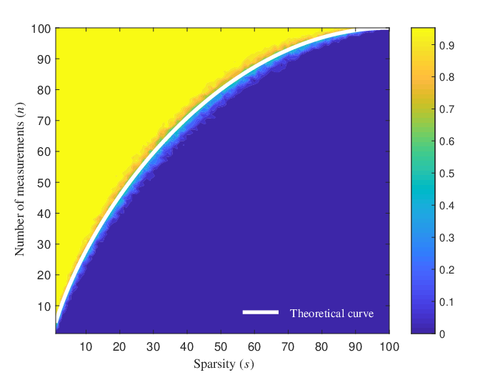
Many CS works have focused on when exact recovery is possible using (12) and how these conditions change as a function of the problem parameters. Early works such as [21] observed that the probability of exact recovery possesses a phase transition with respect to the number of measurements, $n$, and the sparsity of the signal, $s$. Here, a phase transition means a dramatic change in the probability of exact recovery when these parameters, $n$ and $s$, vary around certain values. To illustrate the phase transition phenomenon associated with the probability of exact recovery, we empirically present in Fig. 1 the probabilities of exact recovery, assuming an under-determined real-valued Gaussian measurement matrix $\bm{\Psi}$, applying (12) under different pairs $(n,s)$. The corresponding phase transition points $(n,s)$ where phase transitions happen, compose what we call the phase transition curve. This curve precisely characterizes the required conditions for exact recovery. While empirically calculating the curve is usually time consuming, expressions of the theoretical curve have been given in certain cases as we discuss next.

The paper [19] identified a theoretical phase transition curve for a more general optimization problem of the form

under a real-valued Gaussian measurement matrix $\bm{\Psi}$, based on integral geometry techniques. Here, $f(\cdot)$ is restricted to be convex and does not take the value $-\infty$. In general, $f(\cdot)$ indicates the ‘structure’ in a vector. For example, $f(\cdot)=\lVert\cdot\rVert_{1}$ characterizes the standard sparsity of a vector, and in this case (14) reduces to (12). To calculate the number of measurements $n$ which causes a phase transition, two concepts are introduced, the descent cone and the statistical dimension. The descent cone of a proper convex function $f:\mathbb{R}^{d}\rightarrow\mathbb{R}$ at the point $\bm{x}\in\mathbb{R}^{d}$ is defined as

It depicts the conic hull of the perturbations which decrease or maintain $f$ around $\bm{x}$. The number of measurements $n$ which causes a phase transition, representing the phase transition curve, depends on the descent cone at the point $\bm{x}$, given by

Here, $\delta(\cdot)$ is called the statistical dimension of a cone, the expectation is taken over the random vector $\bm{g}\in\mathbb{R}^{d}$, obeying the Gaussian distribution $\bm{g}\thicksim\mathscr{N}(\bm{0},\bm{I})$, and ${\rm dist}(x,S)$ denotes the Euclidean distance from a vector $\bm{x}\in\mathbb{R}^{d}$ to a set $S\subset\mathbb{R}^{d}$

Now, identifying the phase transition curve becomes calculating the statistical dimension with respect to the $\ell_{1}$ norm.

To apply Proposition 1, we substitute $f(\cdot)$ with $\|\cdot\|_{1}$ in (19) and calculate the infimum distance expectation $J(\bm{x},\|\cdot\|_{1})$, which implies the upper bound on $\delta(D(\|\cdot\|_{1},\bm{x}))$. We then express the upper bound as a function of the sparsity and the dimension of $\bm{x}$, $s$ and $d$, as claimed in the following proposition:

Consider the model in (13) with $\bm{y}\in\mathbb{R}^{n}$, $\bm{\Psi}\in\mathbb{R}^{n\times md}$ and $\bm{x}\in\mathbb{R}^{md}$. Here, we assume that $\bm{\Psi}$ is a real-valued Gaussian matrix and $\bm{x}$ is block sparse with sparsity $s_{B}$. According to Proposition 1, we let $f(\bm{x})$ be the $\ell_{2,1}$ norm of $\bm{x}$ with a block size $m$. Thus, the phase transition curve becomes $\delta(D(\|\cdot\|_{2,1},\bm{x}))$ and can be achieved by calculating the term in the right hand side of (19) with respect to $f(\bm{x})$. Following the steps used for the derivation of Proposition 2, we obtain the following proposition, which provides an upper bound on $\delta(D(\|\cdot\|_{2,1},\bm{x}))$ in terms of $s_{B}$ and $d$.

Proposition 3 offers a theoretical bound on the phase transition curve in block sparse recovery, which is empirically tight as will be shown in Section VI by experiments. It generalizes Proposition 2, because standard $\ell_{1}$ norm minimization can be regarded as a special case of block sparse recovery with $m=1$ and $s_{B}=s$. In this case, the curve $\varphi_{m}(s_{B},d)$ becomes identical to $\varphi(s,d)$ in Proposition 2. Proposition 3 also paves the way to discussing sparse recovery with complex-valued measurement matrices. This is because both $\ell_{1}$ and $\ell_{2,1}$ norm minimization under complex-valued measurement matrices can be expressed by $\ell_{2,1}$ norm minimization in real-valued formulations, as discussed in the next subsection.

It is well known that complex-valued sparse recovery problems can be reformulated into real-valued ones [24]. We use the same model (13) with Subsection IV-A except that variables are complex valued: $\bm{y}\in\mathbb{C}^{n}$, $\bm{x}\in\mathbb{C}^{md}$, and $\bm{\Psi}\in\mathbb{C}^{n\times md}$ being a complex-valued Gaussian matrix. The model can be converted into a real-valued form $\bm{y}_{r}=\bm{\Psi}_{r}\bm{x}_{r}$ by introducing notations: $\bm{y}_{r}:=\left[\Re\bm{y}^{T},\Im\bm{y}^{T}\right]^{T}\in\mathbb{R}^{2n}$, $\bm{\Psi}_{r}:=\begin{bmatrix}\Re\bm{\Psi}&-\Im\bm{\Psi}\\ \Im\bm{\Psi}&\Re\bm{\Psi}\end{bmatrix}\in\mathbb{R}^{2n\times 2md}$ and $\bm{x}_{r}:=\left[\Re\bm{x}^{T},\Im\bm{x}^{T}\right]^{T}\in\mathbb{R}^{2md}$. The $q$-th block in $\bm{x}$ is rewritten as $\bar{\bm{x}}_{q}=\left[\Re\bm{x}_{q}^{T},\Im\bm{x}_{q}^{T}\right]^{T}\in\mathbb{R}^{2m}$. We then exchange the entries in $\bm{x}_{r}$ such that we obtain $\bar{\bm{x}}:=\left[\bar{\bm{x}}_{0}^{T},\dots,\bar{\bm{x}}_{d-1}^{T}\right]^{T}\in\mathbb{R}^{2md}$. Applying the same arrangement to the columns of $\bm{\Psi}_{r}$ yields $\overline{\bm{\Psi}}\in\mathbb{R}^{2n\times 2md}$, and we have $\bm{y}_{r}=\overline{\bm{\Psi}}\bar{\bm{x}}$. Here, the real-valued vector $\bar{\bm{x}}$ has $d$ blocks, which each contains $2m$ entries. The block sparsity of $\bar{\bm{x}}$ remains unchanged, $s_{B}$. Define the $\ell_{2,1}$ norm of $\bar{\bm{x}}$ with respect to the block size $2m$, i.e., $\lVert\bar{\bm{x}}\rVert_{2,1}:=\sum_{q=0}^{d-1}\lVert\bar{\bm{x}}_{q}\rVert_{2}$. Then, it can be verified that $\lVert{\bar{\bm{x}}}_{q}\rVert_{2}=\lVert{\bm{x}}_{q}\rVert_{2}$ and hence $\lVert\bar{\bm{x}}\rVert_{2,1}=\lVert{\bm{x}}\rVert_{2,1}$, where we recall that the latter $\ell_{2,1}$ norm is defined with respect to the block size of $m$. Consequently, the original complex-valued model (13) is equivalent to the optimization problem

Since $\ell_{1}$-norm based sparse recovery is a special case of block sparse recovery, following the same steps, we find that complex-valued $\ell_{1}$ norm minimization is equivalent to a real-valued $\ell_{2,1}$ norm minimization with block width of 2.

We now calculate the bound on $\delta(D(\|\cdot\|_{2,1},\bm{x}))$ for the complex-valued case, based on the real-valued representation (23). Proposition 1 assumes that entries in the measurement matrix are mutually independent Gaussian variables, while $\bm{\Psi}_{r}$ or $\overline{\bm{\Psi}}$ has duplicate entries, which are not independent. However, the dependence introduced by $\bm{\Psi}_{r}$ has little impact on its phase transition curve according to the empirical results in [24], which inspires us to apply Proposition 3, derived from Proposition 1, for the real-valued optimization problem (23). Therefore, the phase transitions of the optimization problem (23) emerge when $2n=\varphi_{2m}(s_{B},d)$, where $\varphi_{m}(s,d)$ is defined in (21). We then denote by

an approximate bound on the phase transition curve. The accuracy of (24) will be verified in Section VI. It provides the location of phase transitions in complex-valued block sparse recovery, which can be applied to standard sparse recovery as well.

Assuming only $N_{b}$ observations out of the whole $N$ radar echoes are available, we use (24) to identify the required $N_{b}$ for exact target reconstruction with block sparse recovery. Substituting $n=N_{b}$, $m=M$, $d=N$ and $s_{B}=K$ into (24), we have

The tightness of (25) makes it a powerful tool for guiding waveform design and evaluating recovery performance of far. For given system parameters $M$ and $N$, as well as $K$, which means that we have some prior knowledge on the number of targets in a single crr bin, (25) provides the minimum requirement on the number of observations to guarantee unique recovered targets. This is particularly useful when one aims to reduce the number of transmitted pulses $N_{b}$ out of $N$, for the purposes of lowering power consumption [6], facilitating spectrum sharing between radar and communication [27], or interference rejection [26]. For a given tuple of parameters $(M,N,N_{b})$, (25) implies an equation with respect to $K$, the maximum number of recoverable targets, evaluating the performance of radars equipped with these parameters. This equation with respect to $K$ can be efficiently solved by iterative methods, e.g., the bisection method [28], because $N_{b}$ is a monotonic function with respect to $K$, as stated below.

Numerical calculation of (25) involves complicated integration operation, and when $M$ is a slightly large number, the precise calculation of (25) is difficult. To avoid the computational burden and allow real-time calculation in practical scenarios, we approximate and simply (25) under different quantitative relations between $N$ and $K$, as given in the following proposition.

We will show in the next section that when $M\geq 4$, these approximations are quite accurate. Among these three relations between $N$ and $K$, the case of $N/K\gg\sqrt{M}$ is of particular interest, representing that the observed target scene is relatively sparse. We will compare this curve with the counterpart of standard sparse recovery in the next subsection.

To compare far’s recovery performance between non-block and block sparse recovery, i.e., (12) and (13), we also use (24) to indicate the required minimum number of radar echoes, denoted by $N_{s}$, when applying (12). In this case, the “block” size is $m=1$, and the length of $\bm{x}$ is $md=d=MN$. The ‘block’ sparsity becomes $s_{B}=KM$, because each target leads to $M$ nonzero entries in $\bm{x}$. Substituting these variables into (24), we obtain

Similarly to Proposition 5, we have the following proposition that present approximations to (30).

In the sequel, we discuss the obtained bounds when $M$ is reasonably large and the observed target scene is relatively sparse, i.e., $N\gg K$, which occurs in many practical scenarios. Under such conditions, we adopt the approximations (26) and (31).

We first note that the obtained conditions that guarantee unique recovery are tighter than the previous counterparts presented in [13, 12]. The previous results, $K_{b}=O(\frac{N}{M\log(MN)})$ and $K_{s}=O(\sqrt{\frac{N}{M^{2}\log(MN)}})$, (the subscripts denote block and standard sparse recovery, respectively), are based on coherence techniques, which lead to pessimistic bounds. To facilitate the comparison between our results and $K_{b}$, $K_{s}$, we set ${N}_{b1}=N$ and ${N}_{s1}=N$ in (26) and (31), respectively, because the intact observation models are considered in [13, 12], where all $N$ pulses are transmitted, received and processed. Regarding (26), we have $K_{\rm ib}\approx\frac{N}{2M+\sqrt{2M}\log\frac{N}{2\sqrt{M}}}$ for intact block sparse recovery (hence the subscript ‘ib’). Since in practice $N$ is usually not extremely larger than $M$, we have ${2M}\geq\sqrt{2M}\log\frac{N}{2K\sqrt{M}}$. As a consequence, $K_{\rm ib}$ scales as $O\left(N/M\right)$, larger than $O(\frac{N}{M\log(MN)})$, indicating the tightness of $K_{\rm ib}$ over $K_{b}$. Similarly, from (31), we have $K_{\rm is}\approx\frac{N}{2M+M\log N}$ for intact standard sparse recovery (hence the subscript ‘is’), which is simplified as $K_{\rm is}=O(\frac{N}{M\log N})$. In comparison with $K_{s}$, we find $K_{\rm is}$ scales larger than $K_{s}$. We will show by simulations in the next section that the approximations we derive in this section are tight for far, while the previous bounds [13, 12] are quite pessimistic.

The tightness enables these approximations to accurately characterize the recovery performance, and facilitates the performance comparison between block and standard sparse recovery for extended targets. In particular, from (26) and (31), we have $N_{b}=2MK+O\left(K\sqrt{M\log\frac{N}{K\sqrt{M}}}\right)$ and $N_{s}=2MK+O\left(KM\log\frac{N}{K}\right)$, respectively, suggesting $N_{b}<N_{s}$ for reasonably large $M$. This means that for given $(M,N,K)$, i.e., under the same system settings and sparse target scene, block sparse recovery requires less observations to guarantee unique recovery of extended targets, implying that block sparse recovery is generally more suitable for recovering extended targets with far.

This subsection carriers out simulation experiments to inspect the phase transitions on block sparse recovery and the phase transitions in complex-valued Gaussian matrices.

The first experiment considers real-valued block sparse recovery described in (13), where the entries of the observation matrix $\bm{\Psi}\in\mathbb{R}^{n\times md}$ obey i.i.d. $\mathscr{N}(0,1)$. The nonzero entries in $\bm{x}\in\mathbb{R}^{md}$ are 1 or -1 randomly with an identical probability $1/2$. We set $m=4$ and $d=32$, and vary $(s_{B},n)$ to calculate the probabilities of exact recovery. In the second simulation, we test the phase transition in complex-valued non-block sparse recovery (12), which can be solved by real-valued block sparse recovery as discussed in Subsection IV-B. Here, the entries of $\bm{\Psi}\in\mathbb{C}^{n\times d}$ have their real and imaginary parts obeying i.i.d. $\mathscr{N}(0,1)$. There are $s$ nonzero entries in $\bm{x}\in\mathbb{C}^{d}$, whose phases are i.i.d. $U([0,2\pi])$ and amplitudes equal 1. We set $d=100$. In both experiments, 50 trials are performed on each pair $(s_{B},n)$ or $(s,n)$ to calculate the success rates. The results for these two experiments are shown in Fig. 2 (a) and (b). The theoretical curves in (a) and (b) are computed by (21) and (24) with corresponding $m$ and $d$, respectively.

Fig. 2 shows that the theoretical curves conform to empirical phase transitions, which verifies Proposition 3 and (24).

We next verify existence of phase transitions in FAR. Both standard and block sparse recovery methods are tested.

To inspect the phase transition in FAR (10), we randomly select $n$ rows from $\bm{\Theta}\in\mathbb{C}^{N\times MN}$ to form a partial measurement matrix $\hat{\bm{\Theta}}\in\mathbb{C}^{n\times MN}$. The phases of nonzero entries in $\bm{x}$ are i.i.d. $U([0,2\pi])$ and the amplitudes equal 1. Given the observations $\bm{y}=\hat{\bm{\Theta}}\bm{x}$, we use both standard (12) and block (13) sparse recovery to estimate $\bm{x}$. Recall that in standard sparse recovery, the sparsity is $KM$. We set the parameters $M=4$, $N=128$, $\frac{\Delta f}{f_{c}}=0.02$, and use 50 trials to calculate the success rates. The results of (12) and (13) are shown in Fig. 3 (a) and (b), respectively. The theoretical curves are calculated with corresponding $M$ and $N$ by (30) and (25), denoted by ‘$N_{s}$’ and ‘$N_{b}$’, representing standard and block sparse recovery, respectively. For the sake of comparison between these two sparse recovery methods, we depict both theoretical curves in each figure of phase transition results.

From Fig. 3, we see that both theoretical curves well match their corresponding phase transition curves of FAR. Let $N_{s}=N_{b}=N$. The predicted numbers of recoverable targets under this setting are $K=11.1$ and $K=14.7$ for standard and block sparse recovery, respectively, whose corresponding success rates are 0.54 ($K=11,\ n=128$ in Fig. 3 (a)) and 0.50 ($K=14,\ n=128$ in Fig. 3 (b)). These rates are close to the threshold $1/2$ that divides the parameter plane into regions of success and failure, indicating that the obtained values of $K$ are tight. However, the counterparts obtained from [12] and [13] are pessimistically $K=0.4$ and $K=0$, respectively. We also find that the curve of ‘$N_{b}$’ is generally lower than that of ‘$N_{s}$’, revealing that block sparse recovery behaves better than standard sparse recovery in the tested cases.

In this subsection, we will show by simulations that our approximations of the phase transition curves are sufficiently close to the theoretical results, so that we can use them in practical applications to avoid time-consuming calculation.

We compute $N_{b}$ and $N_{s}$ versus $K$ with (25) and (30) to represent the theoretical results under different $N$ and $M$. Then we calculate the values of $N_{b1}$, $N_{b2}$ and $N_{s1}$ in (26), (27) and (31), respectively, to compare with the theoretical results. We set the parameters $(N,M)$ to be (128,4), (128,6), (256,10) and (256,12), and the corresponding results are shown in Fig. 4 (a-d), respectively. Since $N_{b}$ and $N_{s}$ cannot exceed $N$, we restrict their scales between 0 and $N$ in these figures.

From Fig. 4, we see that $N_{s1}$ well approximates $N_{s}$ under all the tested scenarios. As expected in the discussions over Proposition 5, when both $M$ and $K$ are small, $N_{b1}$ is closer to $N_{b}$ than $N_{b2}$, while $N_{b2}$ behaves better in fitting $N_{b}$ when either $M$ or $K$ increases. Fig. 4 also shows that the larger $M$ grows, the more block sparse recovery outperforms the standard counterpart, which is in accordance with our analysis in Section V-C.

References

- [1] Y. Li, T. Huang, X. Xu, Y. Liu, and Y. C. Eldar, “Phase transition in frequency agile radar using compressed sensing,” in 2020 IEEE Radar Conference (RadarConf20), pp. 1–6, 2020.
- [2] S. R. Axelsson, “Analysis of random step frequency radar and comparison with experiments,” IEEE Transactions on Geoscience and Remote Sensing, vol. 45, no. 4, pp. 890–904, 2007.
- [3] J. Yang, J. Thompson, X. Huang, T. Jin, and Z. Zhou, “Random-frequency SAR imaging based on compressed sensing,” IEEE Transactions on Geoscience and Remote Sensing, vol. 51, no. 2, pp. 983–994, 2012.
- [4] L. Wang, T. Huang, and Y. Liu, “Phase compensation and image autofocusing for randomized stepped frequency ISAR,” IEEE Sensors Journal, vol. 19, no. 10, pp. 3784–3796, 2019.
- [5] Z. Liu, X. Wei, and X. Li, “Decoupled isar imaging using rsfw based on twice compressed sensing,” IEEE Transactions on Aerospace and Electronic Systems, vol. 50, no. 4, pp. 3195–3211, 2014.
- [6] D. Ma, N. Shlezinger, T. Huang, Y. Liu, and Y. C. Eldar, “Joint radar-communication strategies for autonomous vehicles: Combining two key automotive technologies,” IEEE Signal Processing Magazine, vol. 37, pp. 85–97, 07 2020.
- [7] D. Cohen, K. V. Mishra, and Y. C. Eldar, “Spectrum sharing radar: Coexistence via xampling,” IEEE Transactions on Aerospace and Electronic Systems, vol. 54, no. 3, pp. 1279–1296, 2017.
- [8] S. Liu, Y. Cao, T. S. Yeo, W. Wu, and Y. Liu, “Adaptive clutter suppression in randomized stepped-frequency radar,” IEEE Transactions on Aerospace and Electronic Systems, p. (Early access), 2020.
- [9] T. Huang, N. Shlezinger, X. Xu, Y. Liu, and Y. C. Eldar, “Majorcom: A dual-function radar communication system using index modulation,” IEEE Transactions on Signal Processing, vol. 68, pp. 3423–3438, 2020.
- [10] Y. Liu, H. Meng, G. Li, and X. Wang, “Range-velocity estimation of multiple targets in randomised stepped-frequency radar,” Electronics Letters, vol. 44, no. 17, pp. 1032–1034, 2008.
- [11] Y. C. Eldar and G. Kutyniok, Compressed sensing: theory and applications. Cambridge university press, 2012.
- [12] T. Huang, Y. Liu, X. Xu, Y. C. Eldar, and X. Wang, “Analysis of frequency agile radar via compressed sensing,” IEEE Transactions on Signal Processing, vol. 66, no. 23, pp. 6228–6240, 2018.
- [13] L. Wang, T. Huang, and Y. Liu, “Theoretical analysis for extended target recovery in randomized stepped frequency radars,” arXiv preprint arXiv:1908.02929, 2019.
- [14] K. Gerlach and M. J. Steiner, “Adaptive detection of range distributed targets,” IEEE Transactions on Signal Processing, vol. 47, no. 7, pp. 1844–1851, 1999.
- [15] Y. C. Eldar, Sampling theory: Beyond bandlimited systems. Cambridge University Press, 2015.
- [16] Y. C. Eldar, P. Kuppinger, and H. Bolcskei, “Block-sparse signals: Uncertainty relations and efficient recovery,” IEEE Transactions on Signal Processing, vol. 58, no. 6, pp. 3042–3054, 2010.
- [17] M. Mishali and Y. C. Eldar, “Reduce and boost: Recovering arbitrary sets of jointly sparse vectors,” IEEE Transactions on Signal Processing, vol. 56, no. 10, pp. 4692–4702, 2008.
- [18] L. Carin, D. Liu, and B. Guo, “Coherence, compressive sensing, and random sensor arrays,” IEEE Antennas and Propagation Magazine, vol. 53, no. 4, pp. 28–39, 2011.
- [19] D. Amelunxen, M. Lotz, M. B. McCoy, and J. A. Tropp, “Living on the edge: Phase transitions in convex programs with random data,” Information and Inference: A Journal of the IMA, vol. 3, no. 3, pp. 224–294, 2014.
- [20] S. Foucart and H. Rauhut, “Sparse recovery with random matrices,” in A Mathematical Introduction to Compressive Sensing, pp. 271–310, Springer, 2013.
- [21] D. L. Donoho, “High-dimensional centrally symmetric polytopes with neighborliness proportional to dimension,” Discrete & Computational Geometry, vol. 35, no. 4, pp. 617–652, 2006.
- [22] M. Stojnic, “Various thresholds for -optimization in compressed sensing,” arXiv preprint arXiv:0907.3666, 2009.
- [23] M. Stojnic, F. Parvaresh, and B. Hassibi, “On the reconstruction of block-sparse signals with an optimal number of measurements,” IEEE Transactions on Signal Processing, vol. 57, no. 8, pp. 3075–3085, 2009.
- [24] Z. Yang, C. Zhang, and L. Xie, “On phase transition of compressed sensing in the complex domain,” IEEE Signal Processing Letters, vol. 19, no. 1, pp. 47–50, 2011.
- [25] D. Donoho and J. Tanner, “Observed universality of phase transitions in high-dimensional geometry, with implications for modern data analysis and signal processing,” Philosophical Transactions of the Royal Society A: Mathematical, Physical and Engineering Sciences, vol. 367, no. 1906, pp. 4273–4293, 2009.
- [26] T. Huang, N. Shlezinger, X. Xu, D. Ma, Y. Liu, and Y. C. Eldar, “Multi-carrier agile phased array radar,” IEEE Transactions on Signal Processing, vol. 68, pp. 5706–5721, 2020.
- [27] D. Ma, N. Shlezinger, T. Huang, Y. Shavit, M. Namer, Y. Liu, and Y. C. Eldar, “Spatial modulation for joint radar-communications systems: Design, analysis, and hardware prototype,” 2020.
- [28] A. Eiger, K. Sikorski, and F. Stenger, “A bisection method for systems of nonlinear equations,” ACM Transactions on Mathematical Software (TOMS), vol. 10, no. 4, pp. 367–377, 1984.
- [29] R. T. Rockafellar, Convex analysis. No. 28, Princeton university press, 1970.
- [30] K. L. Chung, A course in probability theory. Academic press, 2001.
- [31] T. Burić and N. Elezović, “Bernoulli polynomials and asymptotic expansions of the quotient of gamma functions,” J. Comput. Appl. Math., vol. 235, no. 11, p. 3315–3331, 2011.