Joint Air Quality and Weather Predictions Based on Multi-Adversarial Spatiotemporal Networks
Abstract
Accurate and timely air quality and weather predictions are of great importance to urban governance and human livelihood. Though many efforts have been made for air quality or weather prediction, most of them simply employ one another as feature input, which ignores the inner-connection between two predictive tasks. On the one hand, the accurate prediction of one task can help improve another task’s performance. On the other hand, geospatially distributed air quality and weather monitoring stations provide additional hints for city-wide spatiotemporal dependency modeling. Inspired by the above two insights, in this paper, we propose the Multi-adversarial spatiotemporal recurrent Graph Neural Networks (MasterGNN) for joint air quality and weather predictions. Specifically, we first propose a heterogeneous recurrent graph neural network to model the spatiotemporal autocorrelation among air quality and weather monitoring stations. Then, we develop a multi-adversarial graph learning framework to against observation noise propagation introduced by spatiotemporal modeling. Moreover, we present an adaptive training strategy by formulating multi-adversarial learning as a multi-task learning problem. Finally, extensive experiments on two real-world datasets show that MasterGNN achieves the best performance compared with seven baselines on both air quality and weather prediction tasks.
Introduction

With the rapid development of the economy and urbanization, people are increasingly concerned about emerging public health risks and environmental sustainability. As reported by the World Health Organization (WHO), air pollution is the world’s largest environmental health risk (Campbell-Lendrum and Prüss-Ustün 2019), and the changing weather profoundly affects the local economic development and people’s daily life (Baklanov et al. 2018). Thus, accurate and timely air quality and weather predictions are of great importance to urban governance and human livelihood. In the past years, massive sensor stations have been deployed for monitoring air quality (e.g., PM2.5 and PM10) or weather conditions (e.g., temperature and humidity) and many efforts have been made for air quality and weather predictions (Liang et al. 2018; Yi et al. 2018; Wang, Cao, and Yu 2019).
However, existing air quality and weather prediction methods are designated for either air quality or weather prediction, perhaps with one another as a side input (Zheng et al. 2015; Yi et al. 2018), but overlook the intrinsic connections and interactions between two tasks. Different from existing studies, this work is motivated by the following two insights. First, air quality and weather predictions are two highly correlated tasks and can be mutually enhanced. For example, accurately predicting the regional wind condition can help model the future dispersion and transport of air pollutants (Ding, Huang, and Fu 2017). As another example, modeling the future concentration of aerosol pollutants (e.g., PM2.5 and PM10) also can help predict the local climate (e.g., temperature and humidity), since aerosol elements can scatter or absorb the incoming radiation (Hong et al. 2020). Second, as illustrated in Figure 1, the geospatially distributed air quality and weather monitoring stations provide additional hints to improve both predictive tasks. The air quality and weather condition variations in different city locations reflect the urban dynamics and can be exploited to improve spatiotemporal autocorrelation modeling.
In this work, we investigate the joint prediction of air quality and weather conditions by explicitly modeling the correlations and interactions between two predictive tasks. However, two major challenges arise in achieving this goal. (1) Observation heterogeneity. As illustrated in Figure 1, the geo-distributed air quality and weather stations are heterogeneous spatial objects that are monitoring exclusively different atmospheric conditions. Existing methods (Zheng, Liu, and Hsieh 2013; Wang, Cao, and Yu 2019) are initially designed to model homogeneous spatial objects (i.e., either air quality or weather stations), which are not suitable for joint air quality and weather predictions. Therefore, the first challenge is how to capture spatiotemporal autocorrelations among heterogeneous monitoring stations to mutually benefit air quality and weather prediction. (2) Compounding observation error vulnerability. In practice, observations reported by monitoring stations are often noisy due to the sensor error and environmental interference (Yi et al. 2016). However, most existing prediction models (Zheng et al. 2015; Liang et al. 2018; Yi et al. 2018) rely on spatiotemporal dependency modeling between stations, which is susceptible to local perturbations and noise propagation (Zügner, Akbarnejad, and Günnemann 2018; Bengio et al. 2015). More severely, jointly modeling spatiotemporal autocorrelation among air quality and weather monitoring stations will further accumulate errors from both spatial and temporal domains. As a result, it is challenging to learn robust representations to resist compounding observation error for joint air quality and weather predictions.
To tackle the above challenges, we propose the Multi-adversarial spatiotemporal recurrent Graph Neural Networks (MasterGNN) for robust air quality and weather joint predictions. Specifically, we first devise a heterogeneous recurrent graph neural network to simultaneously incorporate spatial and temporal autocorrelations among heterogeneous stations conditioned on dynamic urban contextual factors (e.g., POI distributions, traffics). Then, we propose a multi-adversarial learning framework to against noise propagation from both microscopic and macroscopic perspectives. By proactively simulating perturbations and maximizing the divergence between target and fake observations, multiple discriminators dynamically regularize air quality and weather station representations to resist the propagation of observation noises (Durugkar, Gemp, and Mahadevan 2016). Moreover, we introduce a multi-task adaptive training strategy to improve the joint prediction performance by automatically balancing the importance of multiple discriminators. Finally, we conduct extensive experiments on two real-world datasets collected from Beijing and Shanghai, and the proposed model consistently outperforms seven baselines on both air quality and weather prediction tasks.
Preliminaries
Consider a set of monitoring stations , where and are respectively air quality and weather station sets. Each station is associated with a geographical location (i.e., latitude and longitude) and a set of time-invariant contextual features .
Definition 1.
Observations. Given a monitoring station , the observations of at time step are defined as , which is a vector of air-quality or weather conditions, depending on the station type.
Note that the observations of two types of monitoring stations are different (e.g., PM2.5 and CO in air quality stations, while temperature and humidity in weather stations) and the observation dimensionality of the air quality station and the weather station are also different. We use to denote time-dependent observations of all stations in a time period , use and to respectively denote observations of air quality and weather stations at time step . We use to denote all observations of station . In the following, without ambiguity, we will omit the superscript and subscript.
Problem Statement.
Joint air quality and weather predictions. Given a set of monitoring stations , contextual features , and historical observations , our goal at a time step is to simultaneously predict air quality and weather conditions for all over the next time steps,
| (1) |
where is the estimated target observations of all stations at time step , and is the mapping function we aim to learn. Note that is also station type dependent, i.e., air quality or weather observations for corresponding stations.
Methodology
MasterGNN simultaneously makes air quality and weather predictions based on the following intuitions.
Intuition 1: Heterogeneous spatiotemporal autocorrelation modeling. The geo-distributed air quality and weather monitoring stations provide additional spatiotemporal hints for air quality and weather prediction. The model should be able to simultaneously incorporate spatial and temporal autocorrelations of such heterogeneous monitoring stations for joint air quality and weather prediction.
Intuition 2: Robust representation learning. The spatiotemporal autocorrelation based joint prediction model is vulnerable to observation noises and suffers from compounding propagation errors. The model should be robust to error propagation from both spatial and temporal domains.
Intuition 3: Adaptive model training. Learning robust representations introduces extra optimization objectives, which guiding the predictive model to approximate the underlying data distribution from different semantic aspects. The model should be able to balance the optimization of multiple objectives for optimal prediction adaptively.
Framework Overview
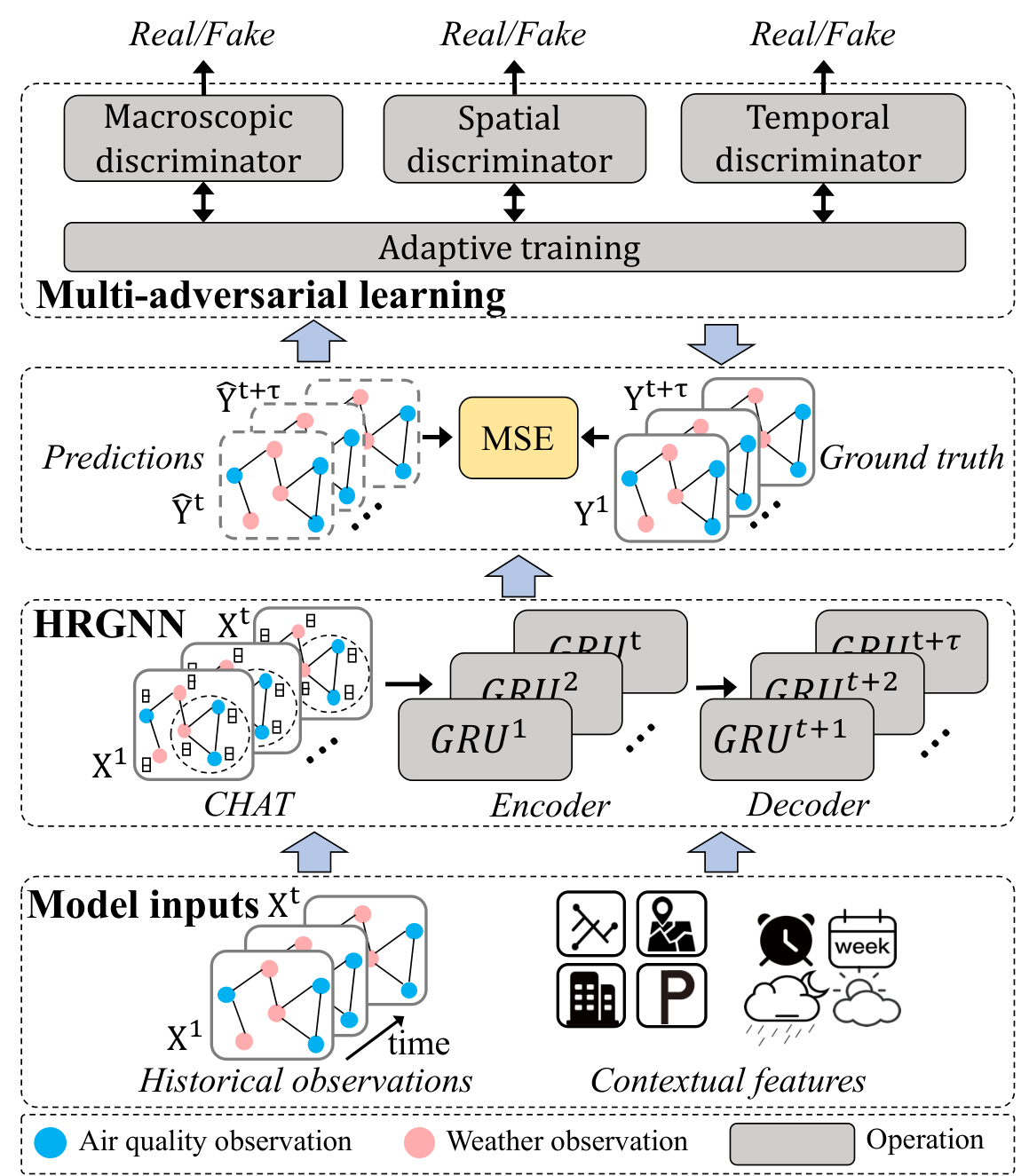
Figure 2 shows the architecture of our approach, including three major tasks: (i) modeling the spatiotemporal autocorrelation among air quality and weather stations for joint prediction; (ii) learning robust station representations via multi-adversarial learning; (iii) exploiting adaptive training strategy to ease the model learning. Specifically, in the first task, we propose a Heterogeneous Recurrent Graph Neural Network (HRGNN) to jointly incorporate spatial autocorrelation between heterogeneous monitoring stations and past-current temporal autocorrelation of each monitoring station. In the second task, we develop a Multi-Adversarial Learning framework to resist the propagation of observation noises via (i) microscopic discriminators against adversarial attacks respectively from the spatial and temporal domain, and (ii) macroscopic discriminator against adversarial attacks from a global view of the city. In the third task, we introduce a Multi-Task Adaptive Training strategy to automatically balance the optimization of multiple discriminative losses in multi-adversarial learning.
Heterogeneous Recurrent Graph Neural Network
The base model.
We adopt the encoder-decoder architecture (Zhang et al. 2020a; Zhang et al. 2020b) as the base model. Specifically, the encoder step projects the historical observation sequence of all stations to a hidden state , where is parameterized by a neural network. In the decoder step, we employ another neural network to generate air quality and weather predictions , where is the future time steps we aim to predict, and are contextual features (Liu et al. 2020b). Similar with conventional air quality or weather prediction models (Liang et al. 2018; Li et al. 2020), the heterogeneous recurrent graph neural network aims to minimize the Mean Square Error (MSE) between the target observations and predictions,
| (2) |
Incorporating spatial autocorrelation.
In the spatial domain, the regional concentration of air pollutants and weather conditions are highly correlated and mutually influenced. Inspired by the recent variants (Wang et al. 2019b; Zhang et al. 2019; Liu et al. 2021) of graph neural network on handling non-Euclidean semantic dependencies on heterogeneous graphs, we devise a context-aware heterogeneous graph attention block (CHAT) to model spatial interactions between heterogeneous stations. We first construct the heterogeneous station graph to describe the spatial adjacency of each station.
Definition 2.
Heterogeneous station graph. A heterogeneous station graph (HSG) is defined as , where is the set of monitoring stations, is a mapping function indicates the type of each station, and is a set of directed edges indicating the connectivity among monitoring stations, defined as
| (3) |
where is the spherical distance between station and station , is a distance threshold.
Due to the heterogeneity of monitoring stations, there are two types of vertices (air quality station , weather station ) and four types of edges, i.e., -, -, -, -. We use to denote the station type of , and to denote the semantic type of each edge.
Formally, given an observation at a particular time step, we first devise a type-specific transformation layer to project heterogeneous observations into unified feature space, , where is a low-dimensional embedding vector, is a learnable weighted matrix shared by all monitoring stations of type .
Then, we introduce a type-dependent attention mechanism to quantify the non-linear correlation between homogeneous and heterogeneous stations under different contexts. Given a station pair which are connected by an edge of type , the attention score is defined as
| (4) |
where is a concatenation based attention function, are contextual features of station and , is the spherical distance between and , and is the set of type-specific neighbor stations of in . Based on , we define the context-aware heterogeneous graph convolution operation to update the type-wise station representation,
| (5) |
where is the aggregated node representation based on edge type , is a non-linear activation function, is a learnable weighted matrix shared over all edges of type . Finally, we obtain the updated station representation of by concatenating type-specific representations,
| (6) |
where is the concatenation operation. Note that we can stack graph convolution layers to capture the spatial autocorrelation between -hop heterogeneous stations.
Incorporating temporal autocorrelation.
In the temporal domain, the air quality and weather conditions also depend on previous observations. We further extend the Gated Recurrent Units (GRU), a simple variant of recurrent neural network (RNN), to integrate the temporal autocorrelation among heterogeneous observation sequences. Consider a station , given the learned spatial representation at time step , we denote the hidden state of at and as and , respectively. The temporal autocorrelation between and is modeled by
| (7) |
where , denote reset gate and update gate at time stamp t, , , , , , are trainable parameters shared by all same-typed monitoring stations, and represents the Hadardmard product.
Multi-Adversarial Learning
We further introduce the multi-adversarial learning framework to obtain robust station representations. By proactively simulating and resisting noisy observations via a minmax game between the generator and discriminator (Goodfellow et al. 2014), adversarial learning can make the generator more robust and generalize better to the underlying true distribution . Compared with standard adversarial learning, our multi-adversarial learning framework encourages the generator to make more consistent predictions from both spatial and temporal domains. Specifically, we function the HRGNN as the generator for joint predictions. Moreover, we propose a set of distinct discriminators to distinguish the real observations and predictions from both microscopic and macroscopic perspectives, as detailed below.
Microscopic discriminators.
Microscopic discriminators aims at enforcing the generator to approximate the underlying spatial and temporal distributions, i.e., pair-wise spatial autocorrelation and stepwise temporal autocorrelation.
Spatial discriminator. From the spatial domain, the adversarial perturbation induces the compounding propagation error through the HSG, as illustrated in Figure 3 (a). Consider a time step , the spatial discriminator aims to maximize the accuracy of distinguishing city-wide real observations and predictions at the current time step,
| (8) |
where is parameterized by the context-aware heterogeneous graph attention block in HRGNN followed by a multi-layer perception, and are ground truth observations and predicted conditions of the city, respectively.
Temporal discriminator. From the temporal domain, the adversarial perturbation induces accumulated error for each station from previous time steps. As depicted in Figure 3 (b), the temporal discriminator outputs a probability indicating how likely a observation sequence of a particular station is from the real data distribution rather than the generator .
| (9) |
Different from the spatial discriminator, is parameterized by the temporal block in HRGNN followed by a multi-layer perception. is a sequence of observations in past and future time steps.
Macroscopic discriminator.
As illustrated in Figure 3 (c), we further propose a macroscopic discriminator to capture the globally underlying distribution, denoted by . In particular, the macroscopic discriminator aims to maximize the accuracy of distinguishing the ground truth observations and predictions generated from from a global view,
| (10) |
where is parameterized by a GRU followed by a multi-layer perception. Note that for efficiency concern, the input of is a simple concatenation of observations from all stations in past and future time steps, but other graph convolution operations are also applicable.
Multi-Task Adaptive Training
It is widely recognized that adversarial training suffers from the unstable and mode collapse problem, where the generator is easy to over-optimized for a particular discriminator (Salimans et al. 2016; Neyshabur, Bhojanapalli, and Chakrabarti 2017). To stabilize the multi-adversarial learning and achieve overall accuracy improvement, we introduce a multi-task adaptive training strategy to dynamically re-weight discriminative loss and enforce the generator to perform well in various spatiotemporal aspects.
Specifically, the objective of MasterGNN is to minimize
| (11) |
where (Equation 2) is the predictive loss, (Equation 8-10) are discriminative losses, and is the importance of the corresponding discriminative loss.
Suppose and are intermediate hidden states in discriminator based on real observations and predictions . We measure the divergence between and by , where is an Euclidean distance based similarity function, is the sigmoid function. Intuitively, reflects the hardness of to distinguish the real sample. In each iteration, we re-weight discriminative losses by . In this way, the generator pays more attention to discriminators with a larger room to improve, and will result in better prediction performance.
Experiments
| Data description | Beijing | Shanghai |
|---|---|---|
| # of air quality stations | 35 | 76 |
| # of weather stations | 18 | 11 |
| # of air quality observations | 409,853 | 1,331,520 |
| # of weather observations | 210,824 | 192,720 |
| # of POIs | 900,669 | 1,061,399 |
| # of road segments | 812,195 | 768,336 |
| Model | MAE/SMAPE | |||||||
|---|---|---|---|---|---|---|---|---|
| Beijing | Shanghai | |||||||
| AQI | Temperature | Humidity | Wind speed | AQI | Temperature | Humidity | Wind speed | |
| ARIMA | 54.97/0.925 | 3.26/0.475 | 16.42/0.403 | 1.17/0.637 | 34.36/0.597 | 2.27/0.394 | 11.96/0.267 | 1.35/0.653 |
| LR | 45.27/0.732 | 2.39/0.426 | 9.58/0.296 | 1.04/0.543 | 27.68/0.462 | 1.93/0.342 | 9.53/0.254 | 1.21/0.568 |
| GBRT | 38.36/0.678 | 2.31/0.397 | 8.43/0.254 | 0.93/0.489 | 24.13/0.423 | 1.87/0.329 | 8.91/0.232 | 1.05/0.497 |
| DeepAir | 31.45/0.613 | 2.21/0.375 | 8.25/0.246 | 0.82/0.468 | 18.79/0.297 | 1.79/0.304 | 7.82/0.209 | 0.93/0.516 |
| GeoMAN | 30.04/0.595 | 2.05/0.356 | 8.01/0.223 | 0.71/0.457 | 20.75/0.348 | 1.56/0.261 | 6.45/0.153 | 0.82/0.465 |
| GC-DCRNN | 29.58/0.586 | 2.14/0.364 | 8.14/0.235 | 0.73/0.462 | 18.73/0.305 | 1.61/0.263 | 6.83/0.186 | 0.78/0.462 |
| DUQ | 32.69/0.624 | 2.02/0.348 | 7.97/0.217 | 0.69/0.446 | 22.81/0.364 | 1.42/0.235 | 6.23/0.136 | 0.67/0.442 |
| MasterGNN | 27.45/0.548 | 1.87/0.326 | 7.25/0.184 | 0.64/0.428 | 16.51/0.265 | 1.25/0.213 | 5.64/0.095 | 0.61/0.427 |
Experimental settings
Data description.
We conduct experiments on two real-world datasets collected from Beijing and Shanghai, two metropolises in China. The Beijing dataset is ranged from January 1, 2017, to April 1, 2018, and the Shanghai dataset is ranged from June 1, 2018, to June 1, 2020. Both datasets include (1) air quality observations (i.e., PM2.5, PM10, O3, NO2, SO2, and CO), (2) weather observations and weather forecast (i.e., weather condition, temperature, pressure, humidity, wind speed and wind direction), and (3) urban contextual data (i.e., POI distribution and Road network distribution (Zhu et al. 2016; Liu et al. 2019; Liu et al. 2020a)). The observation data of Beijing dataset is from KDD CUP 201811 1 https://www.biendata.xyz/competition/kdd_2018/data/, and the observation data of Shanghai dataset is crawled from China government websites22 2 http://www.cnemc.cn/en/. All air quality and weather observations are collected by every hour. We associate POI and road network features to each station through an open API provided by an anonymized online map application. Same as existing studies (Yi et al. 2018; Wang, Cao, and Yu 2019), we focus on Air Quality Index (AQI) for air quality prediction, which is derived by the Chinese AQI standard, and temperature, humidity and wind speed for weather prediction. We split the data into training, validation, and testing data by the ratio of 8:1:1. The statistics of two datasets are shown in Table 2.
Implementation details.
Our model and all the deep learning baselines are implemented with PyTorch. All methods are evaluated on a Linux server with 8 NVIDIA Tesla P40 GPUs. We set context-aware heterogeneous graph attention layers . The cell size of the GRU is set to . We set , and the hidden size of the multi-layer perceptron of each discriminator is fixed to . All the learning parameters are initialized with a uniform distribution, and the model is trained by stochastic gradient descent with a learning rate . The activation function used in the hidden layers is LeakyReLU (=0.2). All the baselines use the same input features as ours, except ARIMA excludes contextual features. Each numerical feature is normalized by Z-score. We set and the future time step . For a fair comparison, we carefully fine-tuned the hyper-parameters of each baseline, and use one another historical observations as a part of feature input.
Evaluation metrics.
We use Mean Absolute Error (MAE) and Symmetric Mean Absolute Percentage Error (SMAPE), two widely used metrics (Luo et al. 2019) for evaluation.
Baselines.
We compare the performance of MasterGNN with the following seven baselines:
- •
ARIMA (Brockwell, Davis, and Calder 2002) is a classic time series prediction method utilizes the moving average and auto-regressive component to estimate future trends.
- •
LR uses linear regression (Montgomery, Peck, and Vining 2012) for joint prediction. We concatenate previous observations and contextual features as input.
- •
GBRT is a tree-based model widely used for regression tasks. We adopt an efficient version XGBoost (Chen and Guestrin 2016), and the input feature is same as LR.
- •
GeoMAN (Liang et al. 2018) is a multi-level attention-based network which integrates spatial and temporal attention for geo-sensory time series prediction.
- •
DeepAir (Yi et al. 2018) is a deep learning method for air quality prediction. It combines spatial transformation and distributed fusion components to fuse various urban data.
- •
GC-DCRNN (Lin et al. 2018) leverages a diffusion convolution recurrent neural network to model spatiotemporal dependencies for air quality prediction.
- •
DUQ (Wang et al. 2019a) is an advanced weather forecasting framework that improves numerical weather prediction by using uncertainty quantification.
Overall performance
Table 2 reports the overall performance of MasterGNN and compared baselines on two datasets with respect to MAE and SMAPE. We observe our approach consistently outperforms all the baselines using both metrics, which shows the superiority of MasterGNN. Specifically, our model achieves (7.8%, 8.0%, 10.0%, 7.8%) and (6.9%, 6.7%, 17.9%, 4.2%) improvements beyond the best baseline on MAE and SMAPE on Beijing for (AQI, temperature, humidity, wind speed) prediction, respectively. Similarly, the improvement of MAE and SMAPE on Shanghai are (13.4%, 13.6%, 10.4%, 9.8%) and (12.1%, 10.3%, 43.2%, 3.5%), respectively. Moreover, we observe all deep learning based models outperform statistical learning based approaches by a large margin, which demonstrate the effectiveness of deep neural network for modeling spatiotemporal dependencies. Remarkably, GC-DCRNN performs better than all other baselines for air quality prediction, and DUQ consistently outperforms other baselines for weather prediction. However, they perform relatively poorly on the other task, which indicates their poor generalization capability and further demonstrate the advantage of joint prediction.
Ablation study
Then we study the effectiveness of each module in MasterGNN. Due to the page limit, we only report the results on Beijing by using SMAPE. The results on Beijing using MAE and on Shanghai using both metrics are similar.
Effect of joint prediction. To validate the effectiveness of joint prediction, we compare the following variants of MasterGNN: (1) SLE models two tasks independently without information sharing, (2) CXT models two tasks independently but uses the other observations as a part of contextual features. As depicted in Figure 4(a), we observe a performance gain of CXT by adding the other observation features, but MasterGNN achieves the best performance. Such results demonstrate the advantage of modeling the interactions between two tasks compared with simply adding the other observations as the feature input.
Effect of heterogeneous recurrent graph neural network. We evaluate three variants of HRGNN, (1) RS removes the spatial autocorrelation block from MasterGNN, (2) AP replaces GRU by average pooling, (3) RH handles air quality and weather observations homogeneously. As shown in Figure 4(b), we observe MasterGNN achieves the best performance compared with other variants, demonstrating the benefits of incorporating spatial and temporal autocorrelations for joint air quality and weather prediction.
Effect of multi-adversarial learning. We compare the following variants: (1) STD removes the macro discriminator, (2) SAD removes the micro temporal discriminator, (3) TAD removes the micro spatial discriminators. As shown in Figure 4(c), the macro discriminator is the most influential one, which indicates the importance of defending noises from the global view. Overall, MasterGNN consistently outperforms STD, SAD, and TAD on all tasks by integrating all discriminators, demonstrating the benefits of developing multiple discriminators for joint prediction.
Effect of multi-task adaptive training. To verify the effect of multi-task adaptive training, we develop (1) Average Loss Minimization (ALM) uses the same weight for all discriminators, (2) Fixed Loss Minimization (FLM) sets weighted but fixed importance based on the performance loss of MasterGNN when the corresponding discriminator is removed. As shown in Figure 4(d), we observe performance degradation when we fix each discriminator’s weight, either on average or weighted. Overall, adaptively re-weighting each discriminator’s importance can guide the optimization direction of the generator and lead to better performance.
Parameter sensitivity
We further study the parameter sensitivity of MasterGNN. We report SMAPE on the Beijing dataset. Each time we vary a parameter, we set others to their default values.
First, we vary the input length from 6 to 96. The results are reported in Figure 5(a). As the input length increases, the performance first increases and then gradually decreases. The main reason is that a short sequence cannot provide sufficient temporal periodicity and trend information. But too large input length may introduce noises for future prediction, leading to performance degradation.
Then, we vary from 8 to 128. The results are reported in Figure 5(b). We can observe that the performance first increases and then remains stable. However, too large leads to extra computation overhead. Therefore, set the is enough to achieve a satisfactory result.
After that, to test the impact of the distance threshold in HSG, we vary from 6 to 20. The results are reported in Figure 5(c). As increases, we observe a performance first increase then slightly decrease, which is perhaps because a large integrates too many stations, which introduces more noises during spatial autocorrelation modeling.
Finally, we vary the prediction step from 3 to 48. The results are reported in Figure 5(d). We observe the performance drops rapidly when goes large. The reason perhaps is the uncertainty increases when is large, and it is difficult for the machine learning model to quantify such uncertainty.
Qualitative study

Finally, we qualitatively analyze why MasterGNN can yield better performance on both tasks. Figure 6 (a) shows the distribution of air quality and weather monitoring stations in the Haidian district, Beijing. We perform a case study from 3:00 May 4, 2017, to 3:00 May 5, 2017. First, we take the air quality station as an illustrative example to show how weather stations help air quality prediction. In MasterGNN, the attention score reflects the relative importance of each neighboring station for prediction. Figure 6 (b) visualizes the attention weights of eight neighboring weather stations of . As can be seen, the attention weights of weather stations , and abruptly increase because a strong wind blows through this area, which results in notable air pollutant dispersion in the next five hours. Clearly, the weather stations provide additional knowledge for air quality prediction. Then, we take the weather station to depict air quality stations’ impact on weather prediction. Figure 6 (c) shows the attention weights of neighbouring station of . We observe the nearest air quality station is the most influential station during 5:00 May 4 2017 and 10:00 May 4 2017, while plays a more important role during 15:00 May 4 2017 and 21:00 May 4 2017, corresponding to notable air pollution concentration changes during these periods. The above observations further validate the additional knowledge introduced by the joint modeling of heterogeneous stations for both predictive tasks.
Related work
Air quality and weather prediction. Existing literature on air quality and weather prediction can be categorized into two classes. (1) Numerical-based models make predictions by simulating the dispersion of various air quality or weather elements based on physical laws (Lorenc 1986; Vardoulakis et al. 2003; Liu, Leung, and Barth 2005; Richardson 2007). (2) Learning-based models utilize end-to-end machine learning methods to capture spatiotemporal correlations based on historical observations and various urban contextual data (e.g., POI distributions, traffics) (Chen and Lai 2011; Zheng, Liu, and Hsieh 2013; Cheng et al. 2018). Recently, many deep learning models (Yi et al. 2018; Wang, Cao, and Yu 2019; Lin et al. 2018) have been proposed to enhance the performance of air quality and weather prediction. By leveraging the representation capacity of deep learning for spatiotemporal autocorrelation modeling, learning-based models usually achieve better prediction performance than numerical-based models. Unlike the above approaches, our method explicitly models the correlations and interactions between the air quality and weather prediction task and achieves a better performance.
Adversarial Learning. Adversarial learning (Goodfellow et al. 2014) is an emerging learning paradigm for better capturing the data distribution via a minmax game between a generator and a discriminator. In the past years, adversarial learning has been widely applied to many real-world application domains, such as sequential recommendation (Yu et al. 2017) and graph learning (Wang et al. 2018). Recently, we notice several multi-adversarial frameworks have been proposed for improving image generation tasks (Nguyen et al. 2017; Hoang et al. 2018; Albuquerque et al. 2019). Inspired by the above studies, we extend the multi-adversarial learning paradigm to the environmental science domain and introduce an adaptive training strategy to improve the stability of adversarial learning.
Conclusion
In this paper, we presented MasterGNN, a joint air quality and weather prediction model that explicitly models the correlations and interactions between two predictive tasks. Specifically, we first proposed a heterogeneous recurrent graph neural network to capture spatiotemporal autocorrelation among air quality and weather monitoring stations. Then, we developed a multi-adversarial learning framework to resist observation noise propagation. In addition, an adaptive training strategy is devised to automatically balance the optimization of multiple discriminative losses in multi-adversarial learning. Extensive experimental results on two real-world datasets demonstrate that the performance of MasterGNN on both air quality and weather prediction tasks consistently outperforms seven state-of-the-art baselines.
References
- Albuquerque et al. (2019) Albuquerque, I.; Monteiro, J.; Doan, T.; Considine, B.; Falk, T.; and Mitliagkas, I. 2019. Multi-objective training of Generative Adversarial Networks with multiple discriminators. arXiv preprint arXiv:1901.08680 .
- Baklanov et al. (2018) Baklanov, A.; Grimmond, C. S. B.; Carlson, D.; Terblanche, D.; Tang, X.; Bouchet, V.; Lee, B.; Langendijk, G.; Kolli, R. K.; and Hovsepyan, A. 2018. From urban meteorology, climate and environment research to integrated city services. Urban Climate 23: 330–341.
- Bengio et al. (2015) Bengio, S.; Vinyals, O.; Jaitly, N.; and Shazeer, N. 2015. Scheduled sampling for sequence prediction with recurrent neural networks. In Advances in Neural Information Processing Systems, 1171–1179.
- Brockwell, Davis, and Calder (2002) Brockwell, P. J.; Davis, R. A.; and Calder, M. V. 2002. Introduction to time series and forecasting, volume 2. Springer.
- Campbell-Lendrum and Prüss-Ustün (2019) Campbell-Lendrum, D.; and Prüss-Ustün, A. 2019. Climate change, air pollution and noncommunicable diseases. Bulletin of the World Health Organization 97(2): 160.
- Chen and Lai (2011) Chen, L.; and Lai, X. 2011. Comparison between ARIMA and ANN models used in short-term wind speed forecasting. In 2011 Asia-Pacific Power and Energy Engineering Conference, 1–4.
- Chen and Guestrin (2016) Chen, T.; and Guestrin, C. 2016. Xgboost: A scalable tree boosting system. In Proceedings of the 22nd ACM SIGKDD international conference on knowledge discovery and data mining, 785–794.
- Cheng et al. (2018) Cheng, W.; Shen, Y.; Zhu, Y.; and Huang, L. 2018. A neural attention model for urban air quality inference: Learning the weights of monitoring stations. In Proceedings of the Thirty-Second AAAI Conference on Artificial Intelligence, 2151–2158.
- Ding, Huang, and Fu (2017) Ding, A.; Huang, X.; and Fu, C. 2017. Air pollution and weather interaction in East Asia. In Oxford Research Encyclopedia of Environmental Science.
- Durugkar, Gemp, and Mahadevan (2016) Durugkar, I.; Gemp, I.; and Mahadevan, S. 2016. Generative multi-adversarial networks. arXiv preprint arXiv:1611.01673 .
- Goodfellow et al. (2014) Goodfellow, I.; Pouget-Abadie, J.; Mirza, M.; Xu, B.; Warde-Farley, D.; Ozair, S.; Courville, A.; and Bengio, Y. 2014. Generative adversarial nets. In Advances in neural information processing systems, 2672–2680.
- Hoang et al. (2018) Hoang, Q.; Nguyen, T. D.; Le, T.; and Phung, D. 2018. MGAN: Training generative adversarial nets with multiple generators. In 6th International Conference on Learning Representations.
- Hong et al. (2020) Hong, C.; Zhang, Q.; Zhang, Y.; Davis, S. J.; Zhang, X.; Tong, D.; Guan, D.; Liu, Z.; and He, K. 2020. Weakening aerosol direct radiative effects mitigate climate penalty on Chinese air quality. Nature Climate Change 1–6.
- Li et al. (2020) Li, Y.; Lang, J.; Ji, L.; Zhong, J.; Wang, Z.; Guo, Y.; and He, S. 2020. Weather forecasting using ensemble of spatial-temporal attention network and multi-layer perceptron. Asia-Pacific Journal of Atmospheric Sciences 1–14.
- Liang et al. (2018) Liang, Y.; Ke, S.; Zhang, J.; Yi, X.; and Zheng, Y. 2018. Geoman: Multi-level attention networks for geo-sensory time series prediction. In Proceedings of the Twenty-Seventh International Joint Conference on Artificial Intelligence, 3428–3434.
- Lin et al. (2018) Lin, Y.; Mago, N.; Gao, Y.; Li, Y.; Chiang, Y.-Y.; Shahabi, C.; and Ambite, J. L. 2018. Exploiting spatiotemporal patterns for accurate air quality forecasting using deep learning. In Proceedings of the 26th ACM SIGSPATIAL international conference on advances in geographic information systems, 359–368.
- Liu, Leung, and Barth (2005) Liu, C.-H.; Leung, D. Y.; and Barth, M. C. 2005. On the prediction of air and pollutant exchange rates in street canyons of different aspect ratios using large-eddy simulation. Atmospheric Environment 39(9): 1567–1574.
- Liu et al. (2021) Liu, H.; Han, J.; Fu, Y.; Zhou, J.; Lu, X.; and Xiong, H. 2021. Multi-Modal Transportation Recommendation with Unified Route Representation Learning. Proceedings of the VLDB Endowment 14(3): 342–350.
- Liu et al. (2020a) Liu, H.; Li, Y.; Fu, Y.; Mei, H.; Zhou, J.; Ma, X.; and Xiong, H. 2020a. Polestar: An Intelligent, Efficient and National-Wide Public Transportation Routing Engine. In Proceedings of the 26th ACM SIGKDD International Conference on Knowledge Discovery and Data Mining, 2321–2329.
- Liu et al. (2020b) Liu, H.; Tong, Y.; Han, J.; Zhang, P.; Lu, X.; and Xiong, H. 2020b. Incorporating Multi-Source Urban Data for Personalized and Context-Aware Multi-Modal Transportation Recommendation. IEEE Transactions on Knowledge and Data Engineering .
- Liu et al. (2019) Liu, H.; Tong, Y.; Zhang, P.; Lu, X.; Duan, J.; and Xiong, H. 2019. Hydra: A personalized and context-aware multi-modal transportation recommendation system. In Proceedings of the 25th ACM SIGKDD International Conference on Knowledge Discovery and Data Mining, 2314–2324.
- Lorenc (1986) Lorenc, A. C. 1986. Analysis methods for numerical weather prediction. Quarterly Journal of the Royal Meteorological Society 112(474): 1177–1194.
- Luo et al. (2019) Luo, Z.; Huang, J.; Hu, K.; Li, X.; and Zhang, P. 2019. AccuAir: Winning solution to air quality prediction for KDD Cup 2018. In Proceedings of the 25th ACM SIGKDD International Conference on Knowledge Discovery and Data Mining, 1842–1850.
- Montgomery, Peck, and Vining (2012) Montgomery, D. C.; Peck, E. A.; and Vining, G. G. 2012. Introduction to linear regression analysis, volume 821. John Wiley & Sons.
- Neyshabur, Bhojanapalli, and Chakrabarti (2017) Neyshabur, B.; Bhojanapalli, S.; and Chakrabarti, A. 2017. Stabilizing GAN training with multiple random projections. arXiv preprint arXiv:1705.07831 .
- Nguyen et al. (2017) Nguyen, T.; Le, T.; Vu, H.; and Phung, D. 2017. Dual discriminator generative adversarial nets. In Advances in Neural Information Processing Systems, 2670–2680.
- Richardson (2007) Richardson, L. F. 2007. Weather prediction by numerical process. Cambridge university press.
- Salimans et al. (2016) Salimans, T.; Goodfellow, I.; Zaremba, W.; Cheung, V.; Radford, A.; and Chen, X. 2016. Improved techniques for training gans. In Advances in neural information processing systems, 2234–2242.
- Vardoulakis et al. (2003) Vardoulakis, S.; Fisher, B. E.; Pericleous, K.; and Gonzalez-Flesca, N. 2003. Modelling air quality in street canyons: a review. Atmospheric environment 37(2): 155–182.
- Wang et al. (2019a) Wang, B.; Lu, J.; Yan, Z.; Luo, H.; Li, T.; Zheng, Y.; and Zhang, G. 2019a. Deep Uncertainty Quantification: A Machine Learning Approach for Weather Forecasting. In International Conference on Knowledge Discovery and Data Mining, 2087–2095. ISBN 978-1-4503-6201-6.
- Wang et al. (2018) Wang, H.; Wang, J.; Zhao, M.; Zhang, W.; Zhang, F.; Xie, X.; and Guo, M. 2018. GraphGAN: Graph representation learning with generative adversarial nets. In Proceedings of the Thirty-second AAAI conference on artificial intelligence, 2508–2515.
- Wang, Cao, and Yu (2019) Wang, S.; Cao, J.; and Yu, P. S. 2019. Deep learning for spatio-temporal data mining: A survey. arXiv preprint arXiv:1906.04928 .
- Wang et al. (2019b) Wang, X.; Ji, H.; Shi, C.; Wang, B.; Ye, Y.; Cui, P.; and Yu, P. S. 2019b. Heterogeneous graph attention network. In The World Wide Web Conference, 2022–2032.
- Yi et al. (2018) Yi, X.; Zhang, J.; Wang, Z.; Li, T.; and Zheng, Y. 2018. Deep distributed fusion network for air quality prediction. In Proceedings of the 24th ACM SIGKDD International Conference on Knowledge Discovery and Data Mining, 965–973.
- Yi et al. (2016) Yi, X.; Zheng, Y.; Zhang, J.; and Li, T. 2016. ST-MVL: Filling missing values in geo-sensory time series data. In Proceedings of the Twenty-Fifth International Joint Conference on Artificial Intelligence, 2704–2710.
- Yu et al. (2017) Yu, L.; Zhang, W.; Wang, J.; and Yu, Y. 2017. Seqgan: Sequence generative adversarial nets with policy gradient. In Proceedings of the Thirty-first AAAI conference on artificial intelligence, 2852–2858.
- Zhang et al. (2019) Zhang, C.; Song, D.; Huang, C.; Swami, A.; and Chawla, N. V. 2019. Heterogeneous graph neural network. In Proceedings of the 25th ACM SIGKDD International Conference on Knowledge Discovery and Data Mining, 793–803.
- Zhang et al. (2020a) Zhang, W.; Liu, H.; Liu, Y.; Zhou, J.; and Xiong, H. 2020a. Semi-Supervised City-Wide Parking Availability Prediction via Hierarchical Recurrent Graph Neural Network. IEEE Transactions on Knowledge and Data Engineering 1–1.
- Zhang et al. (2020b) Zhang, W.; Liu, H.; Liu, Y.; Zhou, J.; and Xiong, H. 2020b. Semi-Supervised Hierarchical Recurrent Graph Neural Network for City-Wide Parking Availability Prediction. In Proceedings of the AAAI Conference on Artificial Intelligence, volume 34, 1186–1193.
- Zheng, Liu, and Hsieh (2013) Zheng, Y.; Liu, F.; and Hsieh, H.-P. 2013. U-air: When urban air quality inference meets big data. In Proceedings of the 19th ACM SIGKDD international conference on Knowledge discovery and data mining, 1436–1444.
- Zheng et al. (2015) Zheng, Y.; Yi, X.; Li, M.; Li, R.; Shan, Z.; Chang, E.; and Li, T. 2015. Forecasting fine-grained air quality based on big data. In Proceedings of the 21th ACM SIGKDD International Conference on Knowledge Discovery and Data Mining, 2267–2276.
- Zhu et al. (2016) Zhu, H.; Xiong, H.; Tang, F.; Liu, Q.; Ge, Y.; Chen, E.; and Fu, Y. 2016. Days on market: Measuring liquidity in real estate markets. In Proceedings of the 22nd ACM SIGKDD International Conference on Knowledge Discovery and Data Mining, 393–402.
- Zügner, Akbarnejad, and Günnemann (2018) Zügner, D.; Akbarnejad, A.; and Günnemann, S. 2018. Adversarial attacks on neural networks for graph data. In Proceedings of the 24th ACM SIGKDD International Conference on Knowledge Discovery and Data Mining, 2847–2856.