跳到论文正文
W Papers独立论文阅读器 arXiv:2012.15036 论文正文 计算阅读时间 · 0%
引用这篇论文根据当前论文元数据生成,正式投稿前建议核对。


License: CC BY-NC-ND 4.0
arXiv:2012.15036v1 [cs.LG] 30 Dec 2020

SGD Distributional Dynamics of Three Layer Neural Networks

Victor Luo    Yazhen Wang Affiliation: Department of Statistics, University of Wisconsin-Madison Affiliation: Madison, WI 53706, USA. Email: vluo@wisc.edu, yzwang@stat.wisc.edu Affiliation: Glenn Fung Affiliation: American Family Insurance, 6000 American Parkway Affiliation: Madison, WI 53783, USA. Email: gfung@amfam.com
Abstract

With the rise of big data analytics, multi-layer neural networks have surfaced as one of the most powerful machine learning methods. However, their theoretical mathematical properties are still not fully understood. Training a neural network requires optimizing a non-convex objective function, typically done using stochastic gradient descent (SGD). In this paper, we seek to extend the mean field results of [9] from two-layer neural networks with one hidden layer to three-layer neural networks with two hidden layers. We will show that the SGD dynamics is captured by a set of non-linear partial differential equations, and prove that the distributions of weights in the two hidden layers are independent. We will also detail exploratory work done based on simulation and real-world data.

1 Introduction

Multi-layer neural networks have been an integral part of statistical machine learning since the 1960s. With advancements in technology and large data capacity, they have surfaced as a “jack of all trades” in a broad array of learning tasks. In spite of the success multi-layer neural networks lack deep theoretical understanding based on rigorous mathematical justifications. Training neural networks requires to solve non-convex high-dimensional optimization problems, common approaches rely on the use of stochastic gradient descent (SGD), and the obtained neural networks heavily depend on the SGD performance ([3], [7], [9], [11]). It has been shown in [9] via mean field theory that the SGD distributional dynamics of two-layers neural networks can be described by a non-linear partial differential equation (PDE). This paper extends the mean field results of [9] from two-layer neural networks with one hidden layer to three-layer neural networks with two hidden layers. We will show that the SGD dynamics is captured by a set of non-linear PDEs, and prove that the distributions of weights in the two hidden layers are independent. We will also detail exploratory work done based on simulation and real-world data.

The rest of the paper is organized as follows. Section 2 describes neutral networks and SGD. Section 3 features the theoretical development of SGD distributional dynamics by mean field theory. Section 4 provides simulations and applications to illustrate the numerical performance of the developed methods.

2 Neural networks and SGD

For this paper, we will focus on the supervised learning setting. Assume we are given data points (𝐱i,yi)∈ℝd×ℝ({\bf x}_{i},y_{i})\in\mathbb{R}^{d}\times\mathbb{R}, indexed by i∈ℕi\in\mathbb{N}, which are assumed to be i.i.d. from unknown distribution ℙ\mathbb{P} on ℝd×ℝ\mathbb{R}^{d}\times\mathbb{R}. 𝐱i∈ℝd{\bf x}_{i}\in\mathbb{R}^{d} is a feature vector and yi∈ℝy_{i}\in\mathbb{R} is a label. Denote ℝd\mathbb{R}^{d} as ℝD0\mathbb{R}^{\prescript{}{0}{D}} for simplicity. Our goal is to model the dependence of the label yiy_{i} on the feature vector of 𝐱i{\bf x}_{i} to assign labels to unlabeled examples. In a three layer neural network (two hidden layers), the dependence is modeled as

y^​(𝐱,𝜽)=1N2​∑m=1N2σ∗2​(σ∗1​(𝐱,𝜽1),𝜽m2)\displaystyle\hat{y}({\bf x};{\bm{\theta}})=\frac{1}{\prescript{}{2}{N}}\sum_{m=1}^{\prescript{}{2}{N}}\prescript{}{2}{\sigma}_{*}(\prescript{}{1}{\sigma}_{*}({\bf x},\prescript{}{1}{\bm{\theta}}),\prescript{}{2}{\bm{\theta}}_{m}) (1)

where Ni\prescript{}{i}{N} is the number of hidden units in the iith hidden layer, σ∗i:ℝDi−1×ℝDi→ℝ\prescript{}{i}{\sigma}_{*}:\mathbb{R}^{\prescript{}{i-1}{D}}\times\mathbb{R}^{\prescript{}{i}{D}}\to\mathbb{R} is the activation function for the iith layer, and 𝜽i∈ℝDi\prescript{}{i}{\bm{\theta}}\in\mathbb{R}^{\prescript{}{i}{D}} are parameters in the iith layer, collectively denoted as 𝜽i=(𝜽1i,…,𝜽Nii)\prescript{}{i}{\bm{\theta}}=(\prescript{}{i}{\bm{\theta}}_{1},\dots,\prescript{}{i}{\bm{\theta}}_{\prescript{}{i}{N}}) for i=1,2i=1,2. We will also denote 𝜽=(𝜽1,𝜽2){\bm{\theta}}=(\prescript{}{1}{\bm{\theta}},\prescript{}{2}{\bm{\theta}}) as a vector of all the parameters. Typically, 𝜽ji=(aji,bji,𝐰𝐣𝐢)\prescript{}{i}{\bm{\theta}}_{j}=(\prescript{}{i}{a}_{j},\prescript{}{i}{b}_{j},\prescript{}{i}{\bf w}_{j}), with

σ∗i​(𝐳𝐢−𝟏,𝜽𝐣𝐢)=𝐚𝐣𝐢∗σ⁡(𝐰𝐣𝐢∘𝐳𝐢−𝟏+𝐛𝐣𝐢)\prescript{}{i}{\sigma}_{*}(\prescript{}{i-1}{\bf z};\prescript{}{i}{\bm{\theta}}_{j})=\prescript{}{i}{a}_{j}*\sigma(\prescript{}{i}{\bf w}_{j}\circ\prescript{}{i-1}{\bf z}+\prescript{}{i}{b}_{j})

for 𝐳𝐢−𝟏∈ℝ𝐃𝐢−𝟏\prescript{}{i-1}{\bf z}\in\mathbb{R}^{\prescript{}{i-1}{D}} and some σ:ℝ→ℝ\sigma:\mathbb{R}\to\mathbb{R}, where ∘\circ represents the Hadamard product. In (1), σ∗1​(𝐱,𝜽1)\prescript{}{1}{\sigma}_{*}({\bf x},\prescript{}{1}{\bm{\theta}}) represents the vector of size D1\prescript{}{1}{D} of values produced by the activation function σ∗1\prescript{}{1}{\sigma}_{*} from the input layer towards the first hidden layer. Typically, the parameters 𝜽{\bm{\theta}} are chosen to minimize the risk RN2​(𝜽)=𝔼⁡{ℓ⁡(y,y^​(𝐱,𝜽))}R_{\prescript{}{2}{N}}({\bm{\theta}})=\mathbb{E}\{\ell(y,\hat{y}({\bf x};{\bm{\theta}}))\}, where ℓ:ℝ×ℝ→ℝ\ell:\mathbb{R}\times\mathbb{R}\to\mathbb{R} is a certain loss function. We will focus on the squared loss ℓ⁡(y,y^)=(y−y^)2\ell(y,\hat{y})=(y-\hat{y})^{2}.

We can rewrite the population risk RN2​(𝜽)=𝔼⁡{(y−y^​(𝐱,𝜽))2}R_{\prescript{}{2}{N}}({\bm{\theta}})=\mathbb{E}\{(y-\hat{y}({\bf x};{\bm{\theta}}))^{2}\} as

RN2​(𝜽)\displaystyle R_{\prescript{}{2}{N}}({\bm{\theta}}) =𝔼⁡{(y−y^​(𝐱,𝜽))2}\displaystyle=\mathbb{E}\{(y-\hat{y}({\bf x},{\bm{\theta}}))^{2}\}
=𝔼⁡{y2−2​y​y^​(𝐱,𝜽)+[y^​(𝐱,𝜽)]2}\displaystyle=\mathbb{E}\{y^{2}-2y\hat{y}({\bf x};{\bm{\theta}})+[\hat{y}({\bf x};{\bm{\theta}})]^{2}\}
=𝔼⁡{y2}+2​𝔼​{−y​y^​(𝐱,𝜽)}+𝔼⁡{[y^​(𝐱,𝜽)]2}\displaystyle=\mathbb{E}\{y^{2}\}+2\mathbb{E}\{-y\hat{y}({\bf x};{\bm{\theta}})\}+\mathbb{E}\{[\hat{y}({\bf x};{\bm{\theta}})]^{2}\}
=R#+2N2​∑i=1N2V⁡(𝜽1,𝜽i2)+1N22​∑i,j=1N2U⁡(𝜽1,𝜽i2,𝜽j2)\displaystyle=R_{\#}+\frac{2}{\prescript{}{2}{N}}\sum_{i=1}^{\prescript{}{2}{N}}V(\prescript{}{1}{\bm{\theta}},\prescript{}{2}{\bm{\theta}}_{i})+\frac{1}{\prescript{}{2}{N}^{2}}\sum_{i,j=1}^{\prescript{}{2}{N}}U(\prescript{}{1}{\bm{\theta}},\prescript{}{2}{\bm{\theta}}_{i},\prescript{}{2}{\bm{\theta}}_{j}) (2)

where the constant R#=𝔼​{y2}R_{\#}=\mathbb{E}\{y^{2}\} is the risk of the trivial predictor y^=0\hat{y}=0, and we define potentials V⁡(𝜽1,𝜽2)=−𝔼⁡{y​σ∗2​(σ∗1​(𝐱,𝜽1),𝜽2)}V(\prescript{}{1}{\bm{\theta}},\prescript{}{2}{\bm{\theta}})=-\mathbb{E}\{y\prescript{}{2}{\sigma}_{*}(\prescript{}{1}{\sigma}_{*}({\bf x},\prescript{}{1}{\bm{\theta}}),\prescript{}{2}{\bm{\theta}})\}, U⁡(𝜽1,𝜽12,𝜽22)=𝔼⁡{σ∗2​(σ∗1​(𝐱,𝜽1),𝜽12)​σ∗2​(σ∗1​(𝐱,𝜽1),𝜽22)}U(\prescript{}{1}{\bm{\theta}},\prescript{}{2}{\bm{\theta}}_{1},\prescript{}{2}{\bm{\theta}}_{2})=\mathbb{E}\{\prescript{}{2}{\sigma}_{*}(\prescript{}{1}{\sigma}_{*}({\bf x},\prescript{}{1}{\bm{\theta}}),\prescript{}{2}{\bm{\theta}}_{1})\prescript{}{2}{\sigma}_{*}(\prescript{}{1}{\sigma}_{*}({\bf x},\prescript{}{1}{\bm{\theta}}),\prescript{}{2}{\bm{\theta}}_{2})\}. We note that U⁡(⋅,⋅)U(\cdot,\cdot) is a symmetric positive semidefinite kernel.

RN2​(𝜽)R_{\prescript{}{2}{N}}({\bm{\theta}}) only depends on 𝜽12,…,𝜽N22\prescript{}{2}{\bm{\theta}}_{1},\dots,\prescript{}{2}{\bm{\theta}}_{\prescript{}{2}{N}} through their empirical distribution ρ^(N2)​(𝜼)=1N2​∑i=1N2δ𝜽i2​(𝜼)\hat{\rho}^{(\prescript{}{2}{N})}({\bm{\eta}})=\frac{1}{\prescript{}{2}{N}}\sum_{i=1}^{\prescript{}{2}{N}}\delta_{\prescript{}{2}{\bm{\theta}}_{i}}({\bm{\eta}}), where 𝜼=(𝜼i)1≤i≤N2{\bm{\eta}}=({\bm{\eta}}_{i})_{1\leq i\leq\prescript{}{2}{N}} with

δ𝜽i2​(𝜼)={1i​f​ 𝜼i≤𝜽i2 ​c​o​m​p​o​n​e​n​t−w​i​s​e0o​t​h​e​r​w​i​s​e\delta_{\prescript{}{2}{\bm{\theta}}_{i}}({\bm{\eta}})=\begin{cases}1&if\text{ ${\bm{\eta}}_{i}\leq\prescript{}{2}{\bm{\theta}}_{i}$ }component-wise\\ 0&otherwise\end{cases}

and “passively” also depends on 𝜽1\prescript{}{1}{\bm{\theta}}, the parameters from the first hidden layer.

We then consider a risk function defined for ρ2∈P⁡(ℝD2)\prescript{}{2}{\rho}\in P(\mathbb{R}^{\prescript{}{2}{D}}), where P⁡(Ω)P(\Omega) is the space of probability distributions on Ω\Omega:

R⁡(ρ2)=\displaystyle R(\prescript{}{2}{\rho})= R#+2​∫V⁡(𝜽1,𝜽2)​ρ2​(d​𝜽2)+∫U⁡(𝜽1,𝜽2,𝜽′2)​ρ2​(d​𝜽2)​ρ2​(d​𝜽′2)\displaystyle R_{\#}+2\int V(\prescript{}{1}{\bm{\theta}},\prescript{}{2}{\bm{\theta}})\prescript{}{2}{\rho}(d\prescript{}{2}{\bm{\theta}})+\int U(\prescript{}{1}{\bm{\theta}},\prescript{}{2}{\bm{\theta}},\prescript{}{2}{\bm{\theta}}^{\prime})\prescript{}{2}{\rho}(d\prescript{}{2}{\bm{\theta}})\prescript{}{2}{\rho}(d\prescript{}{2}{\bm{\theta}}^{\prime}) (3)

Essentially, we have that R⁡(ρ2)R(\prescript{}{2}{\rho}) corresponds to the population risk when the number of hidden units in the second hidden layer goes to infinity, and the empirical distribution of parameters ρ^(N2)\hat{\rho}^{(\prescript{}{2}{N})} converges to ρ2\prescript{}{2}{\rho}, respectively. Due to U⁡(⋅,⋅,⋅)U(\cdot,\cdot,\cdot) being positive semidefinite, the risk becomes convex in the limit.

The parameters of neural networks are learned using stochastic gradient descent (SGD) or some variation. For layer jj, this leads to the iteration

𝜽k+1ij=𝜽kij+2​sk​(yk−y^​(𝐱k,𝜽k))​∇𝜽ijσ∗j​(𝐳𝐤𝐢−𝟏,𝜽𝐤𝐢𝐣).\displaystyle\prescript{}{j}{\bm{\theta}}_{i}^{k+1}=\prescript{}{j}{\bm{\theta}}_{i}^{k}+2s_{k}(y_{k}-\hat{y}({\bf x}_{k};{\bm{\theta}}^{k}))\nabla_{\prescript{}{j}{\bm{\theta}}_{i}}\prescript{}{j}{\sigma}_{*}(\prescript{}{i-1}{\bf z}_{k};\prescript{}{j}{\bm{\theta}}_{i}^{k}). (4)

Here, 𝜽kj=(𝜽kij)i≤Nj\prescript{}{j}{\bm{\theta}}^{k}=(\prescript{}{j}{\bm{\theta}}_{i}^{k})_{i\leq\prescript{}{j}{N}} denotes the parameters in hidden layer jj after kk iterations, 𝜽k=(𝜽k1,𝜽k2){\bm{\theta}}^{k}=(\prescript{}{1}{\bm{\theta}}^{k},\prescript{}{2}{\bm{\theta}}^{k}), sks_{k} as the step size, and (𝐳𝐤𝐢−𝟏,𝐲𝐤)(\prescript{}{i-1}{\bf z}_{k},y_{k}) as the kkth example. We make the One-pass Assumption, which assumes that training examples are never revisited. This is equivalent to {(𝐱k,yk)}k≥1\{({\bf x}_{k},y_{k})\}_{k\geq 1} are i.i.d. (𝐱k,yk)∼ℙ({\bf x}_{k},y_{k})\sim\mathbb{P}.

Our goal is to reduce learning in three-layer neural networks to analyzing the PDE systems in the next section. The structure of the differential dynamics in the next section follows very closely to those of the one and two dimensional diffusions partial differential equations, of which there is much mathematical literature. More specifically, we can view the system as gradient flows where the cost function is R⁡(ρ2,ρ1)R(\prescript{}{2}{\rho};\prescript{}{1}{\rho}) in the space (P⁡(ℝD2),W2)(P(\mathbb{R}^{\prescript{}{2}{D}}),W_{2}), probability measures on ℝD2\mathbb{R}^{\prescript{}{2}{D}} with the Wasserstein metric, where the Wasserstein metric is defined as

W2​(ρ1,ρ2)=(infγ∈Γ⁡(ρ1,ρ2)∫‖𝜽1−𝜽2‖22​γ​(d​𝜽1,d​𝜽2))1/2\displaystyle W_{2}(\rho_{1},\rho_{2})=\bigg(\inf_{\gamma\in\Gamma(\rho_{1},\rho_{2})}\int\|{\bm{\theta}}_{1}-{\bm{\theta}}_{2}\|_{2}^{2}\gamma(d{\bm{\theta}}_{1},d{\bm{\theta}}_{2})\bigg)^{1/2} (5)

where Γ⁡(ρ1,ρ2)\Gamma(\rho_{1},\rho_{2}) represents the set of all couplings of ρ1\rho_{1} and ρ2\rho_{2} and ∥⋅∥2\|\cdot\|_{2} is the ℓ2\ell_{2}-norm.

3 Theoretical Work

In this section, our interest is in defining a theoretical framework for the three layer neural network. More specifically, we are interested in establishing marginal distributions for each of the layers, as well as an overarching joint distribution for the entire network. We assume that the step size in the SGD is given by sk=ϵ​ξ​(k​ϵ)s_{k}=\epsilon\xi(k\epsilon) where ξ:ℝ≥0→ℝ≥0\xi:\mathbb{R}_{\geq 0}\to\mathbb{R}_{\geq 0} is a sufficiently regular function. We will also denote ρ1^k(N1)=1N1​∑i=1N1δ𝜽ki1\hat{\prescript{}{1}{\rho}}_{k}^{(\prescript{}{1}{N})}=\frac{1}{\prescript{}{1}{N}}\sum_{i=1}^{\prescript{}{1}{N}}\delta_{\prescript{}{1}{\bm{\theta}}_{i}^{k}} and ρ2^k(N2)=1N2​∑i=1N2δ𝜽ki2\hat{\prescript{}{2}{\rho}}_{k}^{(\prescript{}{2}{N})}=\frac{1}{\prescript{}{2}{N}}\sum_{i=1}^{\prescript{}{2}{N}}\delta_{\prescript{}{2}{\bm{\theta}}_{i}^{k}} as the empirical distribution of parameters in the first and second hidden layer, respectively, after kk SGD steps.

3.1 Theoretical Framework

3.1.1 Joint Distribution

From our background section, we had that

R⁡(ρ2)=\displaystyle R(\prescript{}{2}{\rho})= R#+2​∫V⁡(𝜽1,𝜽2)​ρ2​(d​𝜽2)+∫U⁡(𝜽1,𝜽2,𝜽′2)​ρ2​(d​𝜽2)​ρ2​(d​𝜽′2)\displaystyle R_{\#}+2\int V(\prescript{}{1}{\bm{\theta}},\prescript{}{2}{\bm{\theta}})\prescript{}{2}{\rho}(d\prescript{}{2}{\bm{\theta}})+\int U(\prescript{}{1}{\bm{\theta}},\prescript{}{2}{\bm{\theta}},\prescript{}{2}{\bm{\theta}}^{\prime})\prescript{}{2}{\rho}(d\prescript{}{2}{\bm{\theta}})\prescript{}{2}{\rho}(d\prescript{}{2}{\bm{\theta}}^{\prime}) (6)

We can rewrite this in terms of conditionals by using the Law of Total Expectation (Tower Property) on our potentials V⁡(⋅,⋅)V(\cdot,\cdot) and U⁡(⋅,⋅,⋅)U(\cdot,\cdot,\cdot):

R⁡(ρ2,ρ1)=\displaystyle R(\prescript{}{2}{\rho};\prescript{}{1}{\rho})= R#+2​∫∫V⁡(𝜽1,𝜽2|𝜽1)​ρ1​(d​𝜽1)​ρ2​(d​𝜽2)\displaystyle R_{\#}+2\int\int V(\prescript{}{1}{\bm{\theta}},\prescript{}{2}{\bm{\theta}}|\prescript{}{1}{\bm{\theta}})\prescript{}{1}{\rho}(d\prescript{}{1}{\bm{\theta}})\prescript{}{2}{\rho}(d\prescript{}{2}{\bm{\theta}})
+∫∫⁡U⁡(𝜽1,𝜽2,𝜽′2|𝜽1)​ρ1​(d​𝜽1)​ρ2​(d​𝜽2)​ρ2​(d​𝜽′2)\displaystyle+\int\int U(\prescript{}{1}{\bm{\theta}},\prescript{}{2}{\bm{\theta}},\prescript{}{2}{\bm{\theta}}^{\prime}|\prescript{}{1}{\bm{\theta}})\prescript{}{1}{\rho}(d\prescript{}{1}{\bm{\theta}})\prescript{}{2}{\rho}(d\prescript{}{2}{\bm{\theta}})\prescript{}{2}{\rho}(d\prescript{}{2}{\bm{\theta}}^{\prime}) (7)

where ρ1∈P⁡(ℝD1)\prescript{}{1}{\rho}\in P(\mathbb{R}^{\prescript{}{1}{D}}).

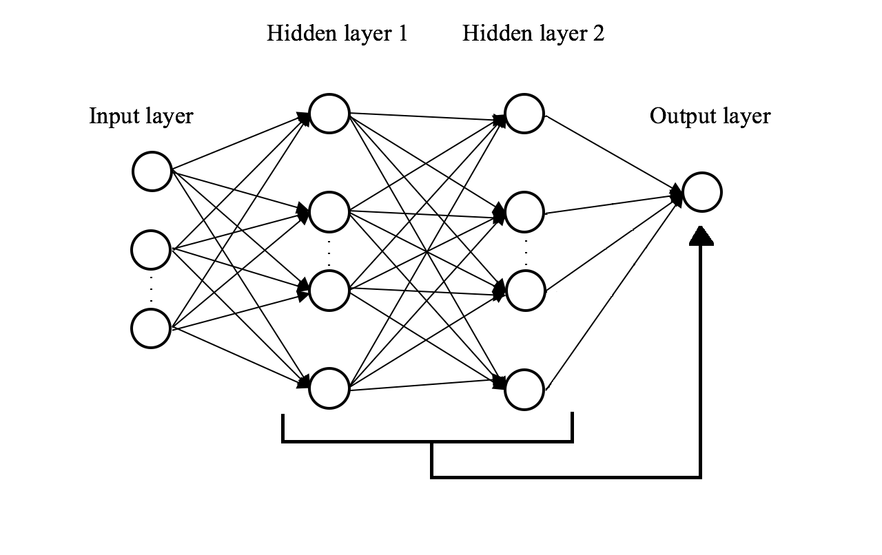
Thus, we can loosely think of R⁡(ρ2,ρ1)R(\prescript{}{2}{\rho};\prescript{}{1}{\rho}) as the joint distribution of the two hidden layers in the neural network towards the output. This is visualized in Figure 1. By taking the partial derivative of R⁡(ρ2,ρ1)R(\prescript{}{2}{\rho};\prescript{}{1}{\rho}) with respect to ρ1\prescript{}{1}{\rho} and ρ2\prescript{}{2}{\rho}, we obtain

R1\displaystyle\prescript{}{1}{R} ≡∂R⁡(ρ2,ρ1)∂ρ2=V⁡(𝜽1,𝜽2)+∫U⁡(𝜽1,𝜽2,𝜽′2)​ρ2​(d​𝜽′2)\displaystyle\equiv\frac{\partial R(\prescript{}{2}{\rho};\prescript{}{1}{\rho})}{\partial\prescript{}{2}{\rho}}=V(\prescript{}{1}{\bm{\theta}},\prescript{}{2}{\bm{\theta}})+\int U(\prescript{}{1}{\bm{\theta}},\prescript{}{2}{\bm{\theta}},\prescript{}{2}{\bm{\theta}}^{\prime})\prescript{}{2}{\rho}(d\prescript{}{2}{\bm{\theta}}^{\prime}) (8)
R2\displaystyle\prescript{}{2}{R} ≡∂R⁡(ρ2,ρ1)∂ρ1=∫V⁡(𝜽1,𝜽2|𝜽1)​ρ2​(d​𝜽2)+∫U⁡(𝜽1,𝜽2,𝜽′2|𝜽1)​ρ2​(d​𝜽2)​ρ2​(d​𝜽′2)\displaystyle\equiv\frac{\partial R(\prescript{}{2}{\rho};\prescript{}{1}{\rho})}{\partial\prescript{}{1}{\rho}}=\int V(\prescript{}{1}{\bm{\theta}},\prescript{}{2}{\bm{\theta}}|\prescript{}{1}{\bm{\theta}})\prescript{}{2}{\rho}(d\prescript{}{2}{\bm{\theta}})+\int U(\prescript{}{1}{\bm{\theta}},\prescript{}{2}{\bm{\theta}},\prescript{}{2}{\bm{\theta}}^{\prime}|\prescript{}{1}{\bm{\theta}})\prescript{}{2}{\rho}(d\prescript{}{2}{\bm{\theta}})\prescript{}{2}{\rho}(d\prescript{}{2}{\bm{\theta}}^{\prime}) (9)
Figure 1: R⁡(ρ2,ρ1)R(\prescript{}{2}{\rho};\prescript{}{1}{\rho}) visualized in neural network.
Refer to caption

Consider R1\prescript{}{1}{R} and R2\prescript{}{2}{R} as the risks in the marginals for layer 1 and 2, respectively. In addition, let ρ1,2\prescript{}{1,2}{\rho} denote the joint density function of 𝜽1\prescript{}{1}{\bm{\theta}} and 𝜽2\prescript{}{2}{\bm{\theta}}. Assume that the marginal densities ρt1\prescript{}{1}{\rho}_{t} and ρt2\prescript{}{2}{\rho}_{t} are independent (⋆\star). Then, we expect the asymptotic dynamics of ρt1,2\prescript{}{1,2}{\rho}_{t} to follow

∂tρt1,2\displaystyle\partial_{t}\prescript{}{1,2}{\rho}_{t} =∂ρt1∂t​ρt2+∂ρt2∂t​ρt1\displaystyle=\frac{\partial\prescript{}{1}{\rho}_{t}}{\partial t}\prescript{}{2}{\rho}_{t}+\frac{\partial\prescript{}{2}{\rho}_{t}}{\partial t}\prescript{}{1}{\rho}_{t} (10)

by the product rule. We will return to this after specifying the marginals.

3.1.2 Marginal Distribution of Second Layer

Turning towards the marginals, we first look at the marginal of the second layer. We can see that the representation in (9) closely resembles the risk function from [9]. Our risk is as follows:

R2​(ρ2|𝜽1)≡∫V⁡(𝜽1,𝜽2|𝜽1)​ρ2​(d​𝜽2)+∫U⁡(𝜽1,𝜽2,𝜽′2|𝜽1)​ρ2​(d​𝜽2)​ρ2​(d​𝜽′2).\displaystyle\prescript{}{2}{R}(\prescript{}{2}{\rho}|\prescript{}{1}{\bm{\theta}})\equiv\int V(\prescript{}{1}{\bm{\theta}},\prescript{}{2}{\bm{\theta}}|\prescript{}{1}{\bm{\theta}})\prescript{}{2}{\rho}(d\prescript{}{2}{\bm{\theta}})+\int U(\prescript{}{1}{\bm{\theta}},\prescript{}{2}{\bm{\theta}},\prescript{}{2}{\bm{\theta}}^{\prime}|\prescript{}{1}{\bm{\theta}})\prescript{}{2}{\rho}(d\prescript{}{2}{\bm{\theta}})\prescript{}{2}{\rho}(d\prescript{}{2}{\bm{\theta}}^{\prime}). (11)

The similarities to the risk function from [9] seem reasonable as we are essentially dealing with a single hidden layer that is directly feeding towards the output layer, which is the type of neural network that [9] was analyzing. It also makes sense for there to be conditioning on 𝜽1\prescript{}{1}{\bm{\theta}} as we are essentially treating the first hidden layer as our input layer in this marginal representation.
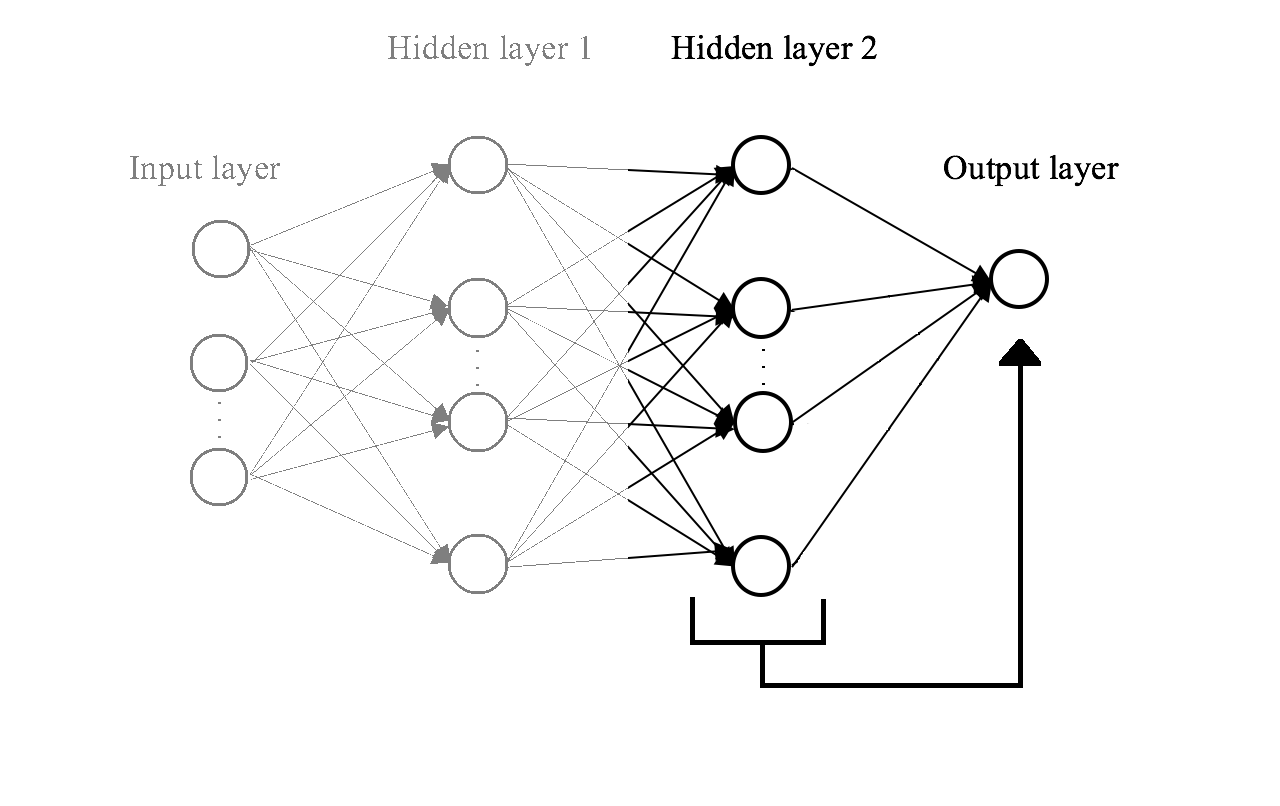
Figure 2: R2​(ρ2)\prescript{}{2}{R}(\prescript{}{2}{\rho}) visualized in neural network.
Refer to caption

Given the conditioning on 𝜽1\prescript{}{1}{\bm{\theta}}, we would then expect the asymptotic dynamics of ρt2|1\prescript{}{2|1}{\rho}_{t}, where ρt2|1\prescript{}{2|1}{\rho}_{t} represents the density of 𝜽2|𝜽1\prescript{}{2}{\bm{\theta}}|\prescript{}{1}{\bm{\theta}}, to follow similar dynamics to those in [9]:

∂tρt2|1\displaystyle\partial_{t}\prescript{}{2|1}{\rho}_{t} =2​ξ​(t)​div𝜽2​{ρt2​∇𝜽2Ψ2|1​(𝜽,ρt2)}\displaystyle=2\xi(t)\text{div}_{\prescript{}{2}{\bm{\theta}}}\{\prescript{}{2}{\rho}_{t}\nabla_{\prescript{}{2}{\bm{\theta}}}\Psi_{2|1}({\bm{\theta}};\prescript{}{2}{\rho}_{t})\} (12)
Ψ2|1​(𝜽,ρ2)\displaystyle\Psi_{2|1}({\bm{\theta}},\prescript{}{2}{\rho}) ≡V⁡(𝜽1,𝜽2|𝜽1)+∫U⁡(𝜽1,𝜽2,𝜽′2|𝜽1)​ρ2​(d​𝜽′2)\displaystyle\equiv V(\prescript{}{1}{\bm{\theta}},\prescript{}{2}{\bm{\theta}}|\prescript{}{1}{\bm{\theta}})+\int U(\prescript{}{1}{\bm{\theta}},\prescript{}{2}{\bm{\theta}},\prescript{}{2}{\bm{\theta}}^{\prime}|\prescript{}{1}{\bm{\theta}})\prescript{}{2}{\rho}(d\prescript{}{2}{\bm{\theta}}^{\prime}) (13)

where div𝜽​{𝐯⁡(𝜽)}\text{div}_{{\bm{\theta}}}\{{\bf v}({\bm{\theta}})\} represents the divergence of the vector field 𝐯⁡(𝜽){\bf v}({\bm{\theta}}). Then, since ∫ρ2|1​ρ1​(d​𝜽1)=ρ2\int\prescript{}{2|1}{\rho}\prescript{}{1}{\rho}(d\prescript{}{1}{\bm{\theta}})=\prescript{}{2}{\rho}, we have that the asymptotic dynamics of ρt2\prescript{}{2}{\rho}_{t} would follow

∂tρt2\displaystyle\partial_{t}\prescript{}{2}{\rho}_{t} =2​ξ​(t)​div𝜽2​{ρt2​∇𝜽2Ψ2​(𝜽,ρt2)}\displaystyle=2\xi(t)\text{div}_{\prescript{}{2}{\bm{\theta}}}\{\prescript{}{2}{\rho}_{t}\nabla_{\prescript{}{2}{\bm{\theta}}}\Psi_{2}({\bm{\theta}};\prescript{}{2}{\rho}_{t})\} (14)
Ψ2​(𝜽,ρ2)\displaystyle\Psi_{2}({\bm{\theta}},\prescript{}{2}{\rho}) ≡V⁡(𝜽1,𝜽2)+∫U⁡(𝜽1,𝜽2,𝜽′2)​ρ2​(d​𝜽′2)\displaystyle\equiv V(\prescript{}{1}{\bm{\theta}},\prescript{}{2}{\bm{\theta}})+\int U(\prescript{}{1}{\bm{\theta}},\prescript{}{2}{\bm{\theta}},\prescript{}{2}{\bm{\theta}}^{\prime})\prescript{}{2}{\rho}(d\prescript{}{2}{\bm{\theta}}^{\prime}) (15)

We are interested in showing that ρt2\prescript{}{2}{\rho}_{t} is a good approximation of ρ^(N2)k2\prescript{}{2}{\hat{\rho}}_{k}^{(\prescript{}{2}{N})}, k=t/ϵk=t/\epsilon, as soon as ϵ<<1/D2\epsilon<<1/\prescript{}{2}{D} and N2>>D2\prescript{}{2}{N}>>\prescript{}{2}{D}.

3.1.3 Marginal Distribution of First Layer

We identify the marginal risk of the first layer as similar to that in (8):

R1​(ρ1)≡V⁡(𝜽1,𝜽2)+∫U⁡(𝜽1,𝜽2,𝜽′2)​ρ2​(d​𝜽′2)\displaystyle\prescript{}{1}{R}(\prescript{}{1}{\rho})\equiv V(\prescript{}{1}{\bm{\theta}},\prescript{}{2}{\bm{\theta}})+\int U(\prescript{}{1}{\bm{\theta}},\prescript{}{2}{\bm{\theta}},\prescript{}{2}{\bm{\theta}}^{\prime})\prescript{}{2}{\rho}(d\prescript{}{2}{\bm{\theta}}^{\prime}) (16)

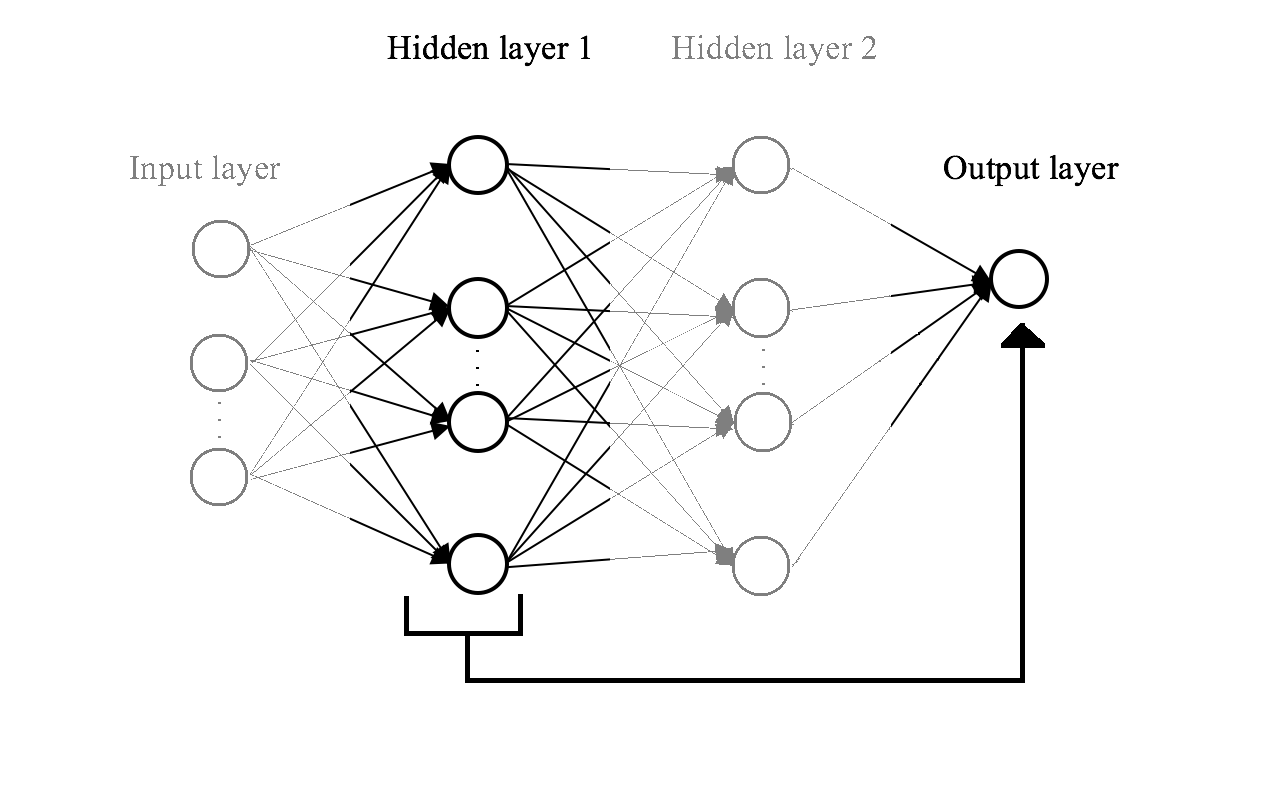
Again, we just have a single hidden layer flowing to an output layer; however, we are still “passively” moving through the second hidden layer (pictured in Figure 3) to get to the final output layer, so we expect the asymptotic dynamics of ρt1|2\prescript{}{1|2}{\rho}_{t}, where ρt1|2\prescript{}{1|2}{\rho}_{t} represents the density of 𝜽1|𝜽2\prescript{}{1}{\bm{\theta}}|\prescript{}{2}{\bm{\theta}}, to follow asymptotic dynamics

∂tρt1|2\displaystyle\partial_{t}\prescript{}{1|2}{\rho}_{t} =2​ξ​(t)​div𝜽1​{ρt1​∇𝜽1Ψ1|2​(𝜽,ρt2)}\displaystyle=2\xi(t)\text{div}_{\prescript{}{1}{\bm{\theta}}}\{\prescript{}{1}{\rho}_{t}\nabla_{\prescript{}{1}{\bm{\theta}}}\Psi_{1|2}({\bm{\theta}};\prescript{}{2}{\rho}_{t})\} (17)
Ψ1|2​(𝜽,ρ2)\displaystyle\Psi_{1|2}({\bm{\theta}},\prescript{}{2}{\rho}) ≡V⁡(𝜽1,𝜽2|𝜽2)+∫U⁡(𝜽1,𝜽2,𝜽′2|𝜽2)​ρ2​(𝜽2)\displaystyle\equiv V(\prescript{}{1}{\bm{\theta}},\prescript{}{2}{\bm{\theta}}|\prescript{}{2}{\bm{\theta}})+\int U(\prescript{}{1}{\bm{\theta}},\prescript{}{2}{\bm{\theta}},\prescript{}{2}{\bm{\theta}}^{\prime}|\prescript{}{2}{\bm{\theta}})\prescript{}{2}{\rho}(\prescript{}{2}{\bm{\theta}}) (18)

where div𝜽​{𝐯⁡(𝜽)}\text{div}_{{\bm{\theta}}}\{{\bf v}({\bm{\theta}})\} represents the divergence of the vector field 𝐯⁡(𝜽){\bf v}({\bm{\theta}}). Then, since ∫ρ1|2​ρ2​(d​𝜽2)=ρ1\int\prescript{}{1|2}{\rho}\prescript{}{2}{\rho}(d\prescript{}{2}{\bm{\theta}})=\prescript{}{1}{\rho}, we have that the asymptotic dynamics of ρt1\prescript{}{1}{\rho}_{t} would follow

∂tρt1\displaystyle\partial_{t}\prescript{}{1}{\rho}_{t} =2​ξ​(t)​div𝜽1​{ρt1​∇𝜽1Ψ1​(𝜽,ρt2)}\displaystyle=2\xi(t)\text{div}_{\prescript{}{1}{\bm{\theta}}}\{\prescript{}{1}{\rho}_{t}\nabla_{\prescript{}{1}{\bm{\theta}}}\Psi_{1}({\bm{\theta}};\prescript{}{2}{\rho}_{t})\} (19)
Ψ1​(𝜽,ρ2)\displaystyle\Psi_{1}({\bm{\theta}},\prescript{}{2}{\rho}) ≡V⁡(𝜽1,𝜽2)+∫U⁡(𝜽1,𝜽2,𝜽′2)​ρ2​(𝜽2)\displaystyle\equiv V(\prescript{}{1}{\bm{\theta}},\prescript{}{2}{\bm{\theta}})+\int U(\prescript{}{1}{\bm{\theta}},\prescript{}{2}{\bm{\theta}},\prescript{}{2}{\bm{\theta}}^{\prime})\prescript{}{2}{\rho}(\prescript{}{2}{\bm{\theta}}) (20)

We are interested in showing that ρt1\prescript{}{1}{\rho}_{t} is a good approximation of ρ^(N1)k1\prescript{}{1}{\hat{\rho}}_{k}^{(\prescript{}{1}{N})}, k=t/ϵk=t/\epsilon, as soon as ϵ<<1/D1\epsilon<<1/\prescript{}{1}{D} and N1>>D1\prescript{}{1}{N}>>\prescript{}{1}{D}.

Figure 3: R1​(ρ1)\prescript{}{1}{R}(\prescript{}{1}{\rho}) visualized in neural network.
Refer to caption

3.1.4 Revisiting the Joint Distribution

From before, under (⋆)(\star), ∂tρt1,2=∂ρt1∂t​ρt2+∂ρt2∂t​ρt1\partial_{t}\prescript{}{1,2}{\rho}_{t}=\frac{\partial\prescript{}{1}{\rho}_{t}}{\partial t}\prescript{}{2}{\rho}_{t}+\frac{\partial\prescript{}{2}{\rho}_{t}}{\partial t}\prescript{}{1}{\rho}_{t}. Combining the results from the previous section, we then have that

∂tρt1,2\displaystyle\partial_{t}\prescript{}{1,2}{\rho}_{t} =2​ξ​(t)​div𝜽​{ρt1,2​∇𝜽Ψ​(𝜽,ρt2)}\displaystyle=2\xi(t)\text{div}_{\bm{\theta}}\{\prescript{}{1,2}{\rho}_{t}\nabla_{\bm{\theta}}\Psi({\bm{\theta}},\prescript{}{2}{\rho}_{t})\} (21)
Ψ⁡(𝜽,ρ2)\displaystyle\Psi({\bm{\theta}},\prescript{}{2}{\rho}) ≡V⁡(𝜽1,𝜽2)+∫U⁡(𝜽1,𝜽2,𝜽′2)​ρ2​(𝜽2)\displaystyle\equiv V(\prescript{}{1}{\bm{\theta}},\prescript{}{2}{\bm{\theta}})+\int U(\prescript{}{1}{\bm{\theta}},\prescript{}{2}{\bm{\theta}},\prescript{}{2}{\bm{\theta}}^{\prime})\prescript{}{2}{\rho}(\prescript{}{2}{\bm{\theta}}) (22)

3.1.5 Simulation Test for Independence of Marginals

In order to get a sense of if (⋆)(\star) has weight to be proven, we first run some simulations to see if there is indeed independence in the weights from the two hidden layers. To test for the independence between the two distributions, we will use the Hoeffding non-parametric independence test, where H0H_{0} is that the two distributions are independent, and HAH_{A} is that they are not independent (see [4]). The Hoeffding DD statistic is calculated as

D\displaystyle D =A−2​(n−2)​B+(n−2)​(n−3)​Cn⁡(n−1)​(n−2)​(n−3)​(n−4)\displaystyle=\frac{A-2(n-2)B+(n-2)(n-3)C}{n(n-1)(n-2)(n-3)(n-4)} (23)
A\displaystyle A =∑α=1naα​(aα−1)​bα​(bα−1)\displaystyle=\sum_{\alpha=1}^{n}a_{\alpha}(a_{\alpha}-1)b_{\alpha}(b_{\alpha}-1) (24)
B\displaystyle B =∑α=1n(aα−1)​(bα−1)​cα\displaystyle=\sum_{\alpha=1}^{n}(a_{\alpha}-1)(b_{\alpha}-1)c_{\alpha} (25)
C\displaystyle C =∑α=1ncα​(cα−1)\displaystyle=\sum_{\alpha=1}^{n}c_{\alpha}(c_{\alpha}-1) (26)
aα\displaystyle a_{\alpha} =∑β=1nγ⁡(Xα−Xβ)−1\displaystyle=\sum_{\beta=1}^{n}\gamma(X_{\alpha}-X_{\beta})-1 (27)
bα\displaystyle b_{\alpha} =∑β=1nγ⁡(Yα−Yβ)−1\displaystyle=\sum_{\beta=1}^{n}\gamma(Y_{\alpha}-Y_{\beta})-1 (28)
cα\displaystyle c_{\alpha} =∑β=1nγ⁡(Xα−Xβ)​γ​(Yα−Yβ)−1\displaystyle=\sum_{\beta=1}^{n}\gamma(X_{\alpha}-X_{\beta})\gamma(Y_{\alpha}-Y_{\beta})-1 (29)

where γ⁡(u)=1\gamma(u)=1 if u≥0u\geq 0, and 0 otherwise and nn is the number of data points we have for each density. P-values on the test statistic DD are approximated by linear interpolation on the table in Hollander and Wolfe, which uses the asymptotically equivalent Blum-Kiefer-Rosenblatt statistic (see [5]).

Table 1: Table comparing p-values from Hoeffding tests.
NN λ\lambda Hidden Nodes per Layer dd mean p-value % of p-values less than 0.05
5000 0.001 100 100 0.396 5%5\%
5000 0.01 100 100 0.420 6%6\%
1000 0.001 100 100 0.364 9%9\%
1000 0.01 100 100 0.407 6%6\%
5000 0.001 100 50 0.375 2%2\%
5000 0.01 100 50 0.408 4%4\%
1000 0.001 100 50 0.403 1%1\%
1000 0.01 100 50 0.406 6%6\%
5000 0.001 50 100 0.413 5%5\%
5000 0.01 50 100 0.405 2%2\%
1000 0.001 50 100 0.410 7%7\%
1000 0.01 50 100 0.391 5%5\%
5000 0.001 50 50 0.437 3%3\%
5000 0.01 50 50 0.388 3%3\%
1000 0.001 50 50 0.409 6%6\%
1000 0.01 50 50 0.410 11%11\%
250 0.001 100 100 0.395 13%13\%
250 0.01 100 100 0.407 7%7\%
250 0.001 100 50 0.436 7%7\%
250 0.01 100 50 0.403 3%3\%

We create a target vector yy of size NN, where yi=1y_{i}=1 with probability 1/21/2 and 00 with probability 1/21/2. Next, we create our covariance matrix, 𝚺{\bm{\Sigma}} of size dd by dd, where the diagonal entries are (1+Δ)2(1+\Delta)^{2} and the off diagonals are 0.0010.001 or 0.010.01 (λ\lambda), and dd is the number of parameters/predictor variables. Then, sample x∼N⁡(0,𝚺)x\sim N(0,{\bf\Sigma}). We will vary NN, λ\lambda, and the number of weights in each hidden layer (the hidden layers will use the same number of nodes). The standard neural network produced in the neuralnet package will be used, only specifying the number of hidden nodes in each layer and the classification parameter (lin.output = TRUE). For each specification of the parameters NN, λ\lambda, dd, and number of hidden nodes in each layer, we run the simulation 100 times and calculate the Hoeffding test each time and record the p-value from each test. The results are produced in Table 1.

From the results, it appears that the two weight distributions are independent in the varying simulations, and our Type I Error for the most part falls in line with our chosen significance level of 0.050.05.

3.2 Convergence Properties

We first want to show that the minimum of the asymptotic risk R⁡(ρ2)R(\prescript{}{2}{\rho}) is a good approximation to minimizing the finite-N2\prescript{}{2}{N} risk RN2​(𝜽)R_{\prescript{}{2}{N}}({\bm{\theta}}).

Proposition 3.1.

Assume one of the following conditions hold:

(a) infρ2R⁡(ρ2)\inf_{\prescript{}{2}{\rho}}R(\prescript{}{2}{\rho}) is achieved by some distribution ρ∗2\prescript{}{2}{\rho}_{*} s.t. ∫U⁡(𝛉1,𝛉2,𝛉′2)​ρ∗2​(d​𝛉2)≤K\int U(\prescript{}{1}{\bm{\theta}},\prescript{}{2}{\bm{\theta}},\prescript{}{2}{\bm{\theta}}^{\prime})\prescript{}{2}{\rho}_{*}(d\prescript{}{2}{\bm{\theta}})\leq K;

(b) ∃ϵ0>0\exists\epsilon_{0}>0 s.t. for any ρ2∈P⁡(ℝD2)\prescript{}{2}{\rho}\in P(\mathbb{R}^{\prescript{}{2}{D}}) s.t. R⁡(ρ2)≤infρ2R⁡(ρ2)+ϵ0R(\prescript{}{2}{\rho})\leq\inf_{\prescript{}{2}{\rho}}R(\prescript{}{2}{\rho})+\epsilon_{0} we have ∫U⁡(𝛉1,𝛉2,𝛉′2)​ρ2​(d​𝛉2)≤K\int U(\prescript{}{1}{\bm{\theta}},\prescript{}{2}{\bm{\theta}},\prescript{}{2}{\bm{\theta}}^{\prime})\prescript{}{2}{\rho}(d\prescript{}{2}{\bm{\theta}})\leq K.

Then,

|inf𝜽2RN2​(𝜽)−infρ2R⁡(ρ2)|≤K/N2.\displaystyle|\inf_{\prescript{}{2}{\bm{\theta}}}R_{\prescript{}{2}{N}}({\bm{\theta}})-\inf_{\prescript{}{2}{\rho}}R({\prescript{}{2}{\rho}})|\leq K/\prescript{}{2}{N}. (30)
Proof.

We see that for any 𝜽2=(𝜽i2)i≤N2\prescript{}{2}{\bm{\theta}}=(\prescript{}{2}{\bm{\theta}}_{i})_{i\leq\prescript{}{2}{N}}, we have that RN2​(𝜽)≥infρ2R⁡(ρ2)R_{\prescript{}{2}{N}}({\bm{\theta}})\geq\inf_{\prescript{}{2}{\rho}}R(\prescript{}{2}{\rho}) where 𝜽=(𝜽1,𝜽2){\bm{\theta}}=(\prescript{}{1}{\bm{\theta}},\prescript{}{2}{\bm{\theta}}). Equality holds when ρ2=1N2​∑i=1nδ𝜽i2\rho_{2}=\frac{1}{\prescript{}{2}{N}}\sum_{i=1}^{n}\delta_{\prescript{}{2}{\bm{\theta}}_{i}}.

Let ρ∗2∈P⁡(ℝD2)\prescript{}{2}{\rho}_{*}\in P(\mathbb{R}^{\prescript{}{2}{D}}) satisfy assumption (a), i.e. ρ∗2\prescript{}{2}{\rho}_{*} achieves infρ2R⁡(ρ2)\inf_{\prescript{}{2}{\rho}}R(\prescript{}{2}{\rho}), or R⁡(ρ2)≤R⁡(ρ∗2)+ϵR(\prescript{}{2}{\rho})\leq R(\prescript{}{2}{\rho}_{*})+\epsilon for any ρ2∈P⁡(RD2)\prescript{}{2}{\rho}\in P(R^{\prescript{}{2}{D}}) under assumption (b). Assume (𝜽i2)i≤N2∼i.i.d.ρ∗2(\prescript{}{2}{\bm{\theta}}_{i})_{i\leq\prescript{}{2}{N}}\sim_{i.i.d.}\prescript{}{2}{\rho}_{*}. Since ∫U⁡(𝜽1,𝜽2,𝜽′2)​ρ∗2​(d​𝜽2)​ρ∗2​(d​𝜽′2)=E⁡{y​(𝐱)2}≥0\int U(\prescript{}{1}{\bm{\theta}},\prescript{}{2}{\bm{\theta}},\prescript{}{2}{\bm{\theta}}^{\prime})\prescript{}{2}{\rho}_{*}(d\prescript{}{2}{\bm{\theta}})\prescript{}{2}{\rho}_{*}(d\prescript{}{2}{\bm{\theta}}^{\prime})=E\{y({\bf x})^{2}\}\geq 0 for y⁡(𝐱)=∫σ∗2​(σ∗1​(𝐱,𝜽1),𝜽2)​ρ∗2​(d​𝜽2)y({\bf x})=\int\prescript{}{2}{\sigma}_{*}(\prescript{}{1}{\sigma}_{*}({\bf x},\prescript{}{1}{\bm{\theta}}),\prescript{}{2}{\bm{\theta}})\prescript{}{2}{\rho}_{*}(d\prescript{}{2}{\bm{\theta}}), we have that

𝔼𝜽2​[RN2​(𝜽)]−R⁡(ρ∗2)\displaystyle\mathbb{E}_{\prescript{}{2}{\bm{\theta}}}[R_{\prescript{}{2}{N}}({\bm{\theta}})]-R(\prescript{}{2}{\rho}_{*}) =1N2{∫U(𝜽1,𝜽2,𝜽′2)ρ∗2(d𝜽2)\displaystyle=\frac{1}{\prescript{}{2}{N}}\bigg\{\int U(\prescript{}{1}{\bm{\theta}},\prescript{}{2}{\bm{\theta}},\prescript{}{2}{\bm{\theta}}^{\prime})\prescript{}{2}{\rho}_{*}(d\prescript{}{2}{\bm{\theta}})
−∫U(𝜽1,𝜽2,𝜽′2)ρ∗2(d𝜽2)ρ∗2(d𝜽′2)}\displaystyle\hskip 28.45274pt-\int U(\prescript{}{1}{\bm{\theta}},\prescript{}{2}{\bm{\theta}},\prescript{}{2}{\bm{\theta}}^{\prime})\prescript{}{2}{\rho}_{*}(d\prescript{}{2}{\bm{\theta}})\prescript{}{2}{\rho}_{*}(d\prescript{}{2}{\bm{\theta}}^{\prime})\bigg\} (31)
≤1N2​∫U⁡(𝜽1,𝜽2,𝜽′2)​ρ∗2​(d​𝜽2)≤KN2,\displaystyle\leq\frac{1}{\prescript{}{2}{N}}\int U(\prescript{}{1}{\bm{\theta}},\prescript{}{2}{\bm{\theta}},\prescript{}{2}{\bm{\theta}}^{\prime})\prescript{}{2}{\rho}_{*}(d\prescript{}{2}{\bm{\theta}})\leq\frac{K}{\prescript{}{2}{N}}, (32)

where the last inequality follows from assumption. Thus,

inf𝜽2RN2​(𝜽)≤R⁡(ρ∗2)+KN2+ϵ.\displaystyle\inf_{\prescript{}{2}{\bm{\theta}}}R_{\prescript{}{2}{N}}({\bm{\theta}})\leq R(\prescript{}{2}{\rho}_{*})+\frac{K}{\prescript{}{2}{N}}+\epsilon. (33)

Since ϵ\epsilon is arbitrary, our claim follows. ∎

Looking towards the PDE systems, we make the following assumptions to establish that the PDE systems describe the limit of the SGD dynamics.

Assumption 1.

t↦ξ⁡(t)t\mapsto\xi(t) is bounded Lipschitz: ‖ξ‖∞,‖ξ‖Lip≤K1\|\xi\|_{\infty},\|\xi\|_{\text{Lip}}\leq K_{1}, with ∫0∞ξ⁡(t)​𝑑t=∞\int_{0}^{\infty}\xi(t)dt=\infty.

Assumption 2.

The activation functions (𝐳,𝛉i)↦σ∗i​(𝐳,𝛉i)({\bf z},\prescript{}{i}{\bm{\theta}})\mapsto\prescript{}{i}{\sigma}_{*}({\bf z};\prescript{}{i}{\bm{\theta}}) are bounded, with sub-Gaussian gradient: ‖σ∗i‖∞≤K2\|\prescript{}{i}{\sigma}_{*}\|_{\infty}\leq K_{2}, ‖∇𝛉iσ∗i​(⋅,𝛉i)‖ψ2≤K2\|\nabla_{\prescript{}{i}{\bm{\theta}}}\prescript{}{i}{\sigma}_{*}(\cdot;\prescript{}{i}{\bm{\theta}})\|_{\psi_{2}}\leq K_{2} for i=1,2i=1,2, where ∥⋅∥ψ2\|\cdot\|_{\psi_{2}} is the Orlicz norm. Labels are also bounded |yk|≤K2|y_{k}|\leq K_{2}.

Assumption 3.

The gradients 𝛉2↦∇𝛉2V​(𝛉1,𝛉2)\prescript{}{2}{\bm{\theta}}\mapsto\nabla_{\prescript{}{2}{\bm{\theta}}}V(\prescript{}{1}{\bm{\theta}},\prescript{}{2}{\bm{\theta}}) and (𝛉2,𝛉′2)↦∇𝛉2U​(𝛉1,𝛉2,𝛉′2)(\prescript{}{2}{\bm{\theta}},\prescript{}{2}{\bm{\theta}}^{\prime})\mapsto\nabla_{\prescript{}{2}{\bm{\theta}}}U(\prescript{}{1}{\bm{\theta}},\prescript{}{2}{\bm{\theta}},\prescript{}{2}{\bm{\theta}}^{\prime}) are bounded, Lipschitz continuous, i.e. we have that ‖∇𝛉2V​(𝛉1,𝛉2)‖2,‖∇𝛉2U​(𝛉1,𝛉2,𝛉′2)‖2≤K3\|\nabla_{\prescript{}{2}{\bm{\theta}}}V(\prescript{}{1}{\bm{\theta}},\prescript{}{2}{\bm{\theta}})\|_{2},\|\nabla_{\prescript{}{2}{\bm{\theta}}}U(\prescript{}{1}{\bm{\theta}},\prescript{}{2}{\bm{\theta}},\prescript{}{2}{\bm{\theta}}^{\prime})\|_{2}\leq K_{3}, ‖∇𝛉2V​(𝛉1,𝛉2)−∇𝛉2V​(𝛉1,𝛉′2)‖2≤K3​‖𝛉2−𝛉′2‖2\|\nabla_{\prescript{}{2}{\bm{\theta}}}V(\prescript{}{1}{\bm{\theta}},\prescript{}{2}{\bm{\theta}})-\nabla_{\prescript{}{2}{\bm{\theta}}}V(\prescript{}{1}{\bm{\theta}},\prescript{}{2}{\bm{\theta}}^{\prime})\|_{2}\leq K_{3}\|\prescript{}{2}{\bm{\theta}}-\prescript{}{2}{\bm{\theta}}^{\prime}\|_{2}, and ‖∇𝛉2U​(𝛉1,𝛉12,𝛉22)−∇𝛉2U​(𝛉1,𝛉′12,𝛉′22)‖2≤K3​‖(𝛉12,𝛉22)−(𝛉′12,𝛉′22)‖2\|\nabla_{\prescript{}{2}{\bm{\theta}}}U(\prescript{}{1}{\bm{\theta}},\prescript{}{2}{\bm{\theta}}_{1},\prescript{}{2}{\bm{\theta}}_{2})-\nabla_{\prescript{}{2}{\bm{\theta}}}U(\prescript{}{1}{\bm{\theta}},\prescript{}{2}{\bm{\theta}}_{1}^{\prime},\prescript{}{2}{\bm{\theta}}_{2}^{\prime})\|_{2}\leq K_{3}\|(\prescript{}{2}{\bm{\theta}}_{1},\prescript{}{2}{\bm{\theta}}_{2})-(\prescript{}{2}{\bm{\theta}}_{1}^{\prime},\prescript{}{2}{\bm{\theta}}_{2}^{\prime})\|_{2}.

With these assumptions, we state the convergence of the SGD process to the PDE model in the second hidden layer and the first hidden layer:

Theorem 3.1.

Assume Assumptions 1, 2, and 3 hold. For ρ0i∈P⁡(ℝDi)\prescript{}{i}{\rho}_{0}\in P(\mathbb{R}^{\prescript{}{i}{D}}) for i=1,2i=1,2, consider SGD with initialization (𝛉j0i)j≤Ni∼i.i.d.ρ0i(\prescript{}{i}{\bm{\theta}}_{j}^{0})_{j\leq{\prescript{}{i}{N}}}\sim_{i.i.d.}\prescript{}{i}{\rho}_{0} and step size sk=ϵ​ξ​(k​ϵ)s_{k}=\epsilon\xi(k\epsilon). For t≥0t\geq 0, let ρt2\prescript{}{2}{\rho}_{t} be the solution of the PDE system from (14) and (15). Then, for any fixed t≥0t\geq 0, ρ^(N2)⌊t/ϵ⌋2⇒ρt2\prescript{}{2}{\hat{\rho}}_{\lfloor t/\epsilon\rfloor}^{(\prescript{}{2}{N})}\Rightarrow\prescript{}{2}{\rho}_{t} almost surely along any sequence (N2,ϵ=ϵN2)(\prescript{}{2}{N},\epsilon=\epsilon_{\prescript{}{2}{N}}) s.t. N→∞N\to\infty, ϵN2→0\epsilon_{\prescript{}{2}{N}}\to 0, N2/log⁡(N2/ϵN2)→∞\prescript{}{2}{N}/\log(\prescript{}{2}{N}/\epsilon_{\prescript{}{2}{N}})\to\infty and ϵN2​log⁡(N2/ϵN2)→0\epsilon_{\prescript{}{2}{N}}\log(\prescript{}{2}{N}/\epsilon_{\prescript{}{2}{N}})\to 0.

Proof.

For this proof, let KK denote a generic constant depending on the constants K1K_{1}, K2K_{2}, and K3K_{3} from Assumptions 1, 2, and 4. From (1), σ∗1​(𝐱,𝜽1)\prescript{}{1}{\sigma}_{*}({\bf x},\prescript{}{1}{\bm{\theta}}) represents the vector of size D1\prescript{}{1}{D} of values produced by the activation function σ∗1\prescript{}{1}{\sigma}_{*} from the input layer towards the first hidden layer. Letting 𝜷k=(σ∗1​(𝐱k,𝜽1),yk){\bm{\beta}}_{k}=(\prescript{}{1}{\sigma}_{*}({\bf x}_{k},\prescript{}{1}{\bm{\theta}}),y_{k}) denote the kkth example, we define

𝐅𝐢𝟐​(𝜽,𝜷𝐤)\displaystyle\prescript{}{2}{\bf F}_{i}({\bm{\theta}};{\bm{\beta}}_{k}) =(yk−y^​(𝐱k,𝜽))​∇𝜽i2σ∗2​(σ∗1​(𝐱k,𝜽1),𝜽i2),𝜽2=(𝜽i2)i≤N2∈ℝD2×N2\displaystyle=\big(y_{k}-{\hat{y}}({\bf x}_{k};{\bm{\theta}})\big)\nabla_{\prescript{}{2}{\bm{\theta}}_{i}}\prescript{}{2}{\sigma}_{*}(\prescript{}{1}{\sigma}_{*}({\bf x}_{k},\prescript{}{1}{\bm{\theta}}),\prescript{}{2}{\bm{\theta}}_{i}),\hskip 56.9055pt\prescript{}{2}{\bm{\theta}}=(\prescript{}{2}{\bm{\theta}}_{i})_{i\leq\prescript{}{2}{N}}\in\mathbb{R}^{\prescript{}{2}{D}\times\prescript{}{2}{N}} (34)
𝐆𝟐​(𝜽,ρ𝟐)\displaystyle\prescript{}{2}{\bf G}({\bm{\theta}};\prescript{}{2}{\rho}) =−∇𝜽2Ψ2​(𝜽,ρ2)=−∇𝜽2V​(𝜽1,𝜽2)−∫∇𝜽2U​(𝜽1,𝜽2,𝜽′2)​ρ2​(d​𝜽′2),𝜽2∈ℝD2.\displaystyle=-\nabla_{\prescript{}{2}{\bm{\theta}}}\Psi_{2}({\bm{\theta}},\prescript{}{2}{\rho})=-\nabla_{\prescript{}{2}{\bm{\theta}}}V(\prescript{}{1}{\bm{\theta}},\prescript{}{2}{\bm{\theta}})-\int\nabla_{\prescript{}{2}{\bm{\theta}}}U(\prescript{}{1}{\bm{\theta}},\prescript{}{2}{\bm{\theta}},\prescript{}{2}{\bm{\theta}}^{\prime})\prescript{}{2}{\rho}(d\prescript{}{2}{\bm{\theta}}^{\prime}),\hskip 28.45274pt\prescript{}{2}{\bm{\theta}}\in\mathbb{R}^{\prescript{}{2}{D}}. (35)

By the assumption of bounded Lipschitz for ∇𝜽2V\nabla_{\prescript{}{2}{\bm{\theta}}}V and ∇𝜽2U\nabla_{\prescript{}{2}{\bm{\theta}}}U, we have that ‖𝐆𝟐​(𝜽,ρ𝟐)‖𝟐≤𝐊\|\prescript{}{2}{\bf G}({\bm{\theta}};\prescript{}{2}{\rho})\|_{2}\leq K and ‖𝐆𝟐​(𝜽𝟏,ρ𝟐)−𝐆𝟐​(𝜽𝟐,ρ𝟐)‖𝟐≤𝐊​‖𝜽𝟏−𝜽𝟐‖𝟐\|\prescript{}{2}{\bf G}({\bm{\theta}}_{1};\prescript{}{2}{\rho})-\prescript{}{2}{\bf G}({\bm{\theta}}_{2};\prescript{}{2}{\rho})\|_{2}\leq K\|{\bm{\theta}}_{1}-{\bm{\theta}}_{2}\|_{2}. In addition,

‖𝐆𝟐​(𝜽,ρ𝟏𝟐)−𝐆𝟐​(𝜽,ρ𝟐𝟐)‖𝟐=‖∫∇𝜽𝟐𝐔​(𝜽𝟏,𝜽𝟐,𝜽′𝟐)​(ρ𝟏𝟐−ρ𝟐𝟐)​(𝐝​𝜽′𝟐)‖𝟐≤𝐊𝐝BL​(ρ𝟏𝟐,ρ𝟐𝟐),\displaystyle\|\prescript{}{2}{\bf G}({\bm{\theta}};\prescript{}{2}{\rho}_{1})-\prescript{}{2}{\bf G}({\bm{\theta}};\prescript{}{2}{\rho}_{2})\|_{2}=\bigg\|\int\nabla_{\prescript{}{2}{\bm{\theta}}}U(\prescript{}{1}{\bm{\theta}},\prescript{}{2}{\bm{\theta}},\prescript{}{2}{\bm{\theta}}^{\prime})(\prescript{}{2}{\rho}_{1}-\prescript{}{2}{\rho}_{2})(d\prescript{}{2}{\bm{\theta}}^{\prime})\bigg\|_{2}\leq Kd_{\text{BL}}(\prescript{}{2}{\rho}_{1},\prescript{}{2}{\rho}_{2}), (36)

where dBL​(⋅,⋅)d_{\text{BL}}(\cdot,\cdot) is the bounded Lipschitz distance between probability measures, i.e.

dBL(μ,η)=sup{|∫f(𝐱)μ(d𝐱)−∫f(𝐱)η(d𝐱)|:∥f∥∞≤1,∥f∥Lip≤1}d_{\text{BL}}(\mu,\eta)=\sup\{|\int f({\bf x})\mu(d{\bf x})-\int f({\bf x})\eta(d{\bf x})|:\|f\|_{\infty}\leq 1,\|f\|_{\text{Lip}}\leq 1\}

and ‖f‖Lip≡supx≠y|f⁡(𝐱)−f⁡(𝐲)|/‖𝐱−𝐲‖2\|f\|_{\text{Lip}}\equiv\sup_{x\not=y}|f({\bf x})-f({\bf y})|/\|{\bf x}-{\bf y}\|_{2}.

We can now rewrite the SGD dynamics in the second layer as

𝜽k+1i2\displaystyle\prescript{}{2}{\bm{\theta}}_{i}^{k+1} =𝜽ki2+2​ϵ​ξ​(k​ϵ)​𝐅𝐢𝟐​(𝜽𝐢𝐤,𝜷𝐤+𝟏)\displaystyle=\prescript{}{2}{\bm{\theta}}_{i}^{k}+2\epsilon\xi(k\epsilon)\prescript{}{2}{\bf F}_{i}({\bm{\theta}}_{i}^{k},{\bm{\beta}}_{k+1}) (37)
⇒𝜽ki2\displaystyle\Rightarrow\prescript{}{2}{\bm{\theta}}_{i}^{k} =𝜽0i2+2​ϵ​∑ℓ=0k−1ξ⁡(ℓ​ϵ)​𝐅𝐢𝟐​(𝜽𝐢ℓ,𝜷ℓ+𝟏).\displaystyle=\prescript{}{2}{\bm{\theta}}_{i}^{0}+2\epsilon\sum_{\ell=0}^{k-1}\xi(\ell\epsilon)\prescript{}{2}{\bf F}_{i}({\bm{\theta}}_{i}^{\ell},{\bm{\beta}}_{\ell+1}). (38)

In order to define nonlinear dynamics to analyze the PDE system for the first layer, we introduce trajectories (𝜽¯ti1,𝜽¯ti2)1,≤i,≤N1,1≤j≤N2,t∈ℝ≥0(\prescript{}{1}{\bar{\bm{\theta}}}_{i}^{t},\prescript{}{2}{\bar{\bm{\theta}}}_{i}^{t})_{1,\leq i,\leq\prescript{}{1}{N},1\leq j\leq\prescript{}{2}{N},t\in\mathbb{R}_{\geq 0}} and letting 𝜽¯i0=𝜽i0{\bar{\bm{\theta}}}_{i}^{0}={\bm{\theta}}_{i}^{0} be the same initialization as for the SGD. Then, for t≥0t\geq 0, the nonlinear dynamics follow

𝜽¯ti2\displaystyle\prescript{}{2}{\bar{\bm{\theta}}}_{i}^{t} =𝜽¯0i2−2​∫0tξ⁡(s)​∇𝜽¯2Ψ2​(𝜽¯is,ρs2)​𝑑s\displaystyle=\prescript{}{2}{\bar{\bm{\theta}}}_{i}^{0}-2\int_{0}^{t}\xi(s)\nabla_{\prescript{}{2}{\bar{\bm{\theta}}}}\Psi_{2}({\bar{\bm{\theta}}}_{i}^{s},\prescript{}{2}{\rho}_{s})ds (39)
ρs2\displaystyle\prescript{}{2}{\rho}_{s} =P𝜽¯si2,\displaystyle=P_{\prescript{}{2}{\bar{\bm{\theta}}}_{i}^{s}}, (40)

where PXP_{X} is the law of the random variable XX. From [10], under Assumptions 1 and 3, the nonlinear dynamics has a unique solution, with ρt2\prescript{}{2}{\rho}_{t} satisfying (14). We notice that under the nonlinear dynamics, the trajectories (𝜽¯ti2)1≤i≤N2,t∈ℝ≥0(\prescript{}{2}{\bar{\bm{\theta}}}_{i}^{t})_{1\leq i\leq\prescript{}{2}{N},t\in\mathbb{R}_{\geq 0}} are i.i.d., which implies that

1N2​∑i=1N2δ𝜽¯ti2⇒ρt2\displaystyle\frac{1}{\prescript{}{2}{N}}\sum_{i=1}^{\prescript{}{2}{N}}\delta_{\prescript{}{2}{\bar{\bm{\theta}}}_{i}^{t}}\Rightarrow\prescript{}{2}{\rho}_{t} (41)

in distribution. We rewrite (39) as

𝜽¯ti2\displaystyle\prescript{}{2}{\bar{\bm{\theta}}}_{i}^{t} =𝜽¯0i2+2​∫0tξ⁡(s)​𝐆𝟐​(𝜽¯𝐢𝐬,ρ𝐬𝟐)​𝐝𝐬\displaystyle=\prescript{}{2}{\bar{\bm{\theta}}}_{i}^{0}+2\int_{0}^{t}\xi(s)\prescript{}{2}{\bf G}({\bar{\bm{\theta}}}_{i}^{s};\prescript{}{2}{\rho}_{s})ds (42)

and compare it to (38). We will define [t]=ϵ​⌊t/ϵ⌋[t]=\epsilon\lfloor t/\epsilon\rfloor for t∈ℝ≥0t\in\mathbb{R}_{\geq 0}. We next detail some Lemmas that bound the difference between the nonlinear dynamics and original dynamics.

Lemma 1.

Assume Assumptions 1 and 3 hold. Let (ρt2)t≥0(\prescript{}{2}{\rho}_{t})_{t\geq 0} be the solution of (14). Let (𝛉¯ti2)t≥0(\prescript{}{2}{\bar{\bm{\theta}}}_{i}^{t})_{t\geq 0} be the solution of (39). Then t↦𝛉¯ti2t\mapsto\prescript{}{2}{\bar{\bm{\theta}}}_{i}^{t} is K1​K3K_{1}K_{3}-Lipschitz continuous, and t↦ρt2t\mapsto\prescript{}{2}{\rho}_{t} is K1​K3K_{1}K_{3}-Lipschitz continuous in W2W_{2} Wasserstein distance.

Proof.

Since ξ\xi is K1K_{1} bounded and ∇𝜽2Ψ2\nabla_{\prescript{}{2}{{\bm{\theta}}}}\Psi_{2} is K3K_{3} bounded, t↦𝜽¯ti2t\mapsto\prescript{}{2}{\bar{\bm{\theta}}}_{i}^{t} is K1​K3K_{1}K_{3}-Lipschitz continuous. In addition, since

dBL​(ρt2,ρs2)≤W2​(ρt2,ρs2)≤(𝔼⁡[‖𝜽¯ti2−𝜽¯si2‖22])1/2≤K1​K3​|t−s|,d_{\text{BL}}(\prescript{}{2}{\rho}_{t},\prescript{}{2}{\rho}_{s})\leq W_{2}(\prescript{}{2}{\rho}_{t},\prescript{}{2}{\rho}_{s})\leq(\mathbb{E}[\|\prescript{}{2}{\bar{\bm{\theta}}}_{i}^{t}-\prescript{}{2}{\bar{\bm{\theta}}}_{i}^{s}\|_{2}^{2}])^{1/2}\leq K_{1}K_{3}|t-s|,

t↦ρt2t\mapsto\prescript{}{2}{\rho}_{t} is Lipschitz continuous in W2W_{2} Wasserstein distance. ∎

Lemma 2.

Under Assumptions 1, 2, 3, ∃\exists constant KK, dependent on K1K_{1}, K2K_{2}, and K3K_{3}, s.t. for any T≥0T\geq 0,

max⁡supℓ∈[0,T/ϵ]∩ℕi≤N2⁡‖𝜽ℓi2−𝜽¯ℓ​ϵi2‖2≤K​T​eK​T​[ϵ+1N2+1/N2∨ϵ​(D2+log⁡(N2​(t/ϵ∨1))+z)]\displaystyle\max_{i\leq\prescript{}{2}{N}}\sup_{\ell\in[0,T/\epsilon]\cap\mathbb{N}}\|\prescript{}{2}{\bm{\theta}}_{i}^{\ell}-\prescript{}{2}{\bar{\bm{\theta}}}_{i}^{\ell\epsilon}\|_{2}\leq KTe^{KT}\bigg[\epsilon+\frac{1}{\prescript{}{2}{N}}+\sqrt{1/\prescript{}{2}{N}\vee\epsilon}\big(\sqrt{\prescript{}{2}{D}+\log(\prescript{}{2}{N}(t/\epsilon\vee 1))}+z\big)\bigg] (43)

with probability at least 1−e−z21-e^{-z^{2}}.

Proof.

We consider t∈ℕ​ϵ∩[0,T]t\in\mathbb{N}\epsilon\cap[0,T] rather than ℓ∈[0,T/ϵ]∩ℕ\ell\in[0,T/\epsilon]\cap\mathbb{N}. If we take the difference in (42) and (38), we have

‖𝜽¯ti2−𝜽t/ϵi2‖2\displaystyle\|\prescript{}{2}{\bar{\bm{\theta}}}_{i}^{t}-\prescript{}{2}{\bm{\theta}}_{i}^{t/\epsilon}\|_{2} =2​‖∫0tξ⁡(s)​𝐆𝟐​(𝜽¯𝐢𝐬,ρ𝐬𝟐)​𝐝𝐬−ϵ​∑ℓ=𝟎𝐭/ϵ−𝟏ξ⁡(ℓ​ϵ)​𝐅𝐢𝟐​(𝜽𝐢ℓ,𝜷ℓ+𝟏)​𝐝𝐬‖𝟐\displaystyle=2\bigg\|\int_{0}^{t}\xi(s)\prescript{}{2}{\bf G}({\bar{\bm{\theta}}}_{i}^{s};\prescript{}{2}{\rho}_{s})ds-\epsilon\sum_{\ell=0}^{t/\epsilon-1}\xi(\ell\epsilon)\prescript{}{2}{\bf F}_{i}({{\bm{\theta}}}_{i}^{\ell};{\bm{\beta}}_{\ell+1})ds\bigg\|_{2} (44)
≤2​∫0t‖ξ⁡(s)​𝐆𝟐​(𝜽¯𝐢𝐬,ρ𝐬𝟐)−ξ⁡([𝐬])​𝐆𝟐​(𝜽¯𝐢[𝐬],ρ[𝐬]𝟐)‖𝟐​𝐝𝐬\displaystyle\leq 2\int_{0}^{t}\bigg\|\xi(s)\prescript{}{2}{\bf G}({\bar{\bm{\theta}}}_{i}^{s};\prescript{}{2}{\rho}_{s})-\xi([s])\prescript{}{2}{\bf G}({\bar{\bm{\theta}}}_{i}^{[s]};\prescript{}{2}{\rho}_{[s]})\bigg\|_{2}ds
+2∫0t∥ξ([s])𝐆𝟐(𝜽¯𝐢[𝐬];ρ[𝐬]𝟐)−ξ([𝐬])𝐆𝟐(𝜽𝐢⌊𝐬/ϵ⌋;ρ[𝐬]𝟐)∥𝟐𝐝𝐬\displaystyle\hskip 28.45274pt+2\int_{0}^{t}\bigg\|\xi([s])\prescript{}{2}{\bf G}({\bar{\bm{\theta}}}_{i}^{[s]};\prescript{}{2}{\rho}_{[s]})-\xi([s])\prescript{}{2}{\bf G}({{\bm{\theta}}}_{i}^{\lfloor s/\epsilon\rfloor};\prescript{}{2}{\rho}_{[s]})\bigg\|_{2}ds
+2​‖ϵ​∑ℓ=0t/ϵ−1ξ⁡(k​ϵ)​{𝐅𝐢𝟐​(𝜽𝐢ℓ,𝜷ℓ+𝟏)−𝐆𝟐​(𝜽𝐢ℓ,ρℓ​ϵ𝟐)}‖𝟐\displaystyle\hskip 28.45274pt+2\bigg\|\epsilon\sum_{\ell=0}^{t/\epsilon-1}\xi(k\epsilon)\big\{\prescript{}{2}{\bf F}_{i}({{\bm{\theta}}}_{i}^{\ell};{\bm{\beta}}_{\ell+1})-\prescript{}{2}{\bf G}({{\bm{\theta}}}_{i}^{\ell};\prescript{}{2}{\rho}_{\ell\epsilon})\big\}\bigg\|_{2} (45)
≡2​Q1i​(t)+2​Q2i​(t)+2​Q3i​(t).\displaystyle\equiv 2Q_{1}^{i}(t)+2Q_{2}^{i}(t)+2Q_{3}^{i}(t). (46)

For the first term Q1i​(t)Q_{1}^{i}(t), we have

Q1i​(t)\displaystyle Q_{1}^{i}(t) ≤tsups∈[0,t]{∥ξ(s)𝐆𝟐(𝜽¯𝐢𝐬;ρ𝐬𝟐)−ξ([𝐬])𝐆𝟐(𝜽¯𝐢𝐬;ρ𝐬𝟐)∥𝟐\displaystyle\leq t\sup_{s\in[0,t]}\bigg\{\|\xi(s)\prescript{}{2}{\bf G}({\bar{\bm{\theta}}}_{i}^{s};\prescript{}{2}{\rho}_{s})-\xi([s])\prescript{}{2}{\bf G}({\bar{\bm{\theta}}}_{i}^{s};\prescript{}{2}{\rho}_{s})\|_{2}
+‖ξ⁡([s])​𝐆𝟐​(𝜽¯𝐢𝐬,ρ𝐬𝟐)−ξ⁡([𝐬])​𝐆𝟐​(𝜽¯𝐢[𝐬],ρ𝐬𝟐)‖𝟐\displaystyle\hskip 28.45274pt+\|\xi([s])\prescript{}{2}{\bf G}({\bar{\bm{\theta}}}_{i}^{s};\prescript{}{2}{\rho}_{s})-\xi([s])\prescript{}{2}{\bf G}({\bar{\bm{\theta}}}_{i}^{[s]};\prescript{}{2}{\rho}_{s})\|_{2}
+∥ξ([s])𝐆𝟐(𝜽¯𝐢[𝐬];ρ𝐬𝟐)−ξ([𝐬])𝐆𝟐(𝜽¯𝐢[𝐬];ρ[𝐬]𝟐)∥𝟐}\displaystyle\hskip 28.45274pt+\|\xi([s])\prescript{}{2}{\bf G}({\bar{\bm{\theta}}}_{i}^{[s]};\prescript{}{2}{\rho}_{s})-\xi([s])\prescript{}{2}{\bf G}({\bar{\bm{\theta}}}_{i}^{[s]};\prescript{}{2}{\rho}_{[s]})\|_{2}\bigg\}
≤K​t​ϵ\displaystyle\leq Kt\epsilon (47)

since 𝐆𝟐​(𝜽,ρ𝟐)\prescript{}{2}{\bf G}({\bm{\theta}};\prescript{}{2}{\rho}) is Lipschitz continuous with respect to 𝜽{\bm{\theta}} and ρ2\prescript{}{2}{\rho} from (36) and by Assumption 1 and Lemma 1 (together implying that ξ\xi, ρs2\prescript{}{2}{\rho}_{s}, and 𝜽¯ti2\prescript{}{2}{\bar{\bm{\theta}}}_{i}^{t} are Lipschitz continuous).

To bound Q2i​(t)Q_{2}^{i}(t), we use Assumption 1 and the Lipschitz continuity of 𝐆𝟐\prescript{}{2}{\bf G} with respect to 𝜽{\bm{\theta}}:

Q2i​(t)≤K​∫0t‖𝐆𝟐​(𝜽¯𝐢[𝐬],ρ[𝐬]𝟐)−𝐆𝟐​(𝜽𝐢⌊𝐬/ϵ⌋,ρ[𝐬]𝟐)‖𝟐​𝐝𝐬≤𝐊𝟐​∫𝟎𝐭‖𝜽¯[𝐬]𝐢𝟐−𝜽⌊𝐬/ϵ⌋𝐢𝟐‖𝟐​𝐝𝐬.\displaystyle Q_{2}^{i}(t)\leq K\int_{0}^{t}\|\prescript{}{2}{\bf G}({\bar{\bm{\theta}}}_{i}^{[s]};\prescript{}{2}{\rho}_{[s]})-\prescript{}{2}{\bf G}({{\bm{\theta}}}_{i}^{\lfloor s/\epsilon\rfloor};\prescript{}{2}{\rho}_{[s]})\|_{2}ds\leq K^{2}\int_{0}^{t}\|\prescript{}{2}{\bar{\bm{\theta}}}_{i}^{[s]}-\prescript{}{2}{{\bm{\theta}}}_{i}^{\lfloor s/\epsilon\rfloor}\|_{2}ds. (48)

To bound Q3i​(t)Q_{3}^{i}(t), we introduce ℱℓ\mathcal{F}_{\ell}, the sigma-algebra generated by (𝜽0i2)i≤N(\prescript{}{2}{{\bm{\theta}}}_{i}^{0})_{i\leq N} and 𝜷1,…,𝜷ℓ{\bm{\beta}}_{1},\dots,{\bm{\beta}}_{\ell} for ℓ∈ℕ\ell\in\mathbb{N}. We see that

𝔼⁡{𝐅𝐢𝟐​(𝜽𝐢ℓ,𝜷ℓ+𝟏)|ℱℓ}=−∇𝜽𝐢𝟐𝐕​(𝜽ℓ𝐢𝟏,𝜽ℓ𝐢𝟐)−𝟏𝐍𝟐​∑𝐣=𝟏𝐍𝟐∇𝜽𝐢𝟐𝐔​(𝜽ℓ𝐢𝟏,𝜽ℓ𝐢𝟐,𝜽ℓ𝐣𝟐)=𝐆𝟐​(𝜽𝐢ℓ,ρ^(𝐍𝟐)ℓ𝟐),\displaystyle\mathbb{E}\big\{\prescript{}{2}{\bf F}_{i}({{\bm{\theta}}}_{i}^{\ell};{\bm{\beta}}_{\ell+1})|\mathcal{F}_{\ell}\big\}=-\nabla_{\prescript{}{2}{\bm{\theta}}_{i}}V(\prescript{}{1}{\bm{\theta}}_{i}^{\ell},\prescript{}{2}{\bm{\theta}}_{i}^{\ell})-\frac{1}{\prescript{}{2}{N}}\sum_{j=1}^{\prescript{}{2}{N}}\nabla_{\prescript{}{2}{\bm{\theta}}_{i}}U(\prescript{}{1}{\bm{\theta}}_{i}^{\ell},\prescript{}{2}{\bm{\theta}}_{i}^{\ell},\prescript{}{2}{\bm{\theta}}_{j}^{\ell})=\prescript{}{2}{\bf G}({\bm{\theta}}_{i}^{\ell};\prescript{}{2}{\hat{\rho}}_{\ell}^{(\prescript{}{2}{N})}), (49)

where ρ^(N2)ℓ2≡1N2​∑i≤N2δ𝜽ℓi2\prescript{}{2}{\hat{\rho}}_{\ell}^{(\prescript{}{2}{N})}\equiv\frac{1}{\prescript{}{2}{N}}\sum_{i\leq\prescript{}{2}{N}}\delta_{\prescript{}{2}{\bm{\theta}}_{i}^{\ell}}. Therefore,

Q3i​(t)\displaystyle Q_{3}^{i}(t) =‖ϵ​∑ℓ=0t/ϵ−1ξ⁡(k​ϵ)​{𝐅𝐢𝟐​(𝜽𝐢ℓ,𝜷ℓ+𝟏)−𝐆𝟐​(𝜽𝐢ℓ,ρℓ​ϵ𝟐)}‖𝟐\displaystyle=\bigg\|\epsilon\sum_{\ell=0}^{t/\epsilon-1}\xi(k\epsilon)\big\{\prescript{}{2}{\bf F}_{i}({{\bm{\theta}}}_{i}^{\ell};{\bm{\beta}}_{\ell+1})-\prescript{}{2}{\bf G}({{\bm{\theta}}}_{i}^{\ell};\prescript{}{2}{\rho}_{\ell\epsilon})\big\}\bigg\|_{2} (50)
≤‖ϵ​∑ℓ=0t/ϵ−1ξ⁡(ℓ​ϵ)​{𝐆𝟐​(𝜽𝐢ℓ,ρ^(𝐍𝟐)ℓ𝟐)−𝐆𝟐​(𝜽𝐢ℓ,ρℓ​ϵ𝟐)}‖𝟐+‖ϵ​∑ℓ=𝟎𝐭/ϵ−𝟏ξ⁡(ℓ​ϵ)​𝐃ℓ𝐢𝟐‖𝟐\displaystyle\leq\bigg\|\epsilon\sum_{\ell=0}^{t/\epsilon-1}\xi(\ell\epsilon)\big\{\prescript{}{2}{\bf G}({\bm{\theta}}_{i}^{\ell};\prescript{}{2}{\hat{\rho}}_{\ell}^{(\prescript{}{2}{N})})-\prescript{}{2}{\bf G}({\bm{\theta}}_{i}^{\ell};\prescript{}{2}{\rho}_{\ell\epsilon})\big\}\bigg\|_{2}+\bigg\|\epsilon\sum_{\ell=0}^{t/\epsilon-1}\xi(\ell\epsilon)\prescript{}{2}{\bf D}_{i}^{\ell}\bigg\|_{2}
≡Q3,0i​(t)+O3,1i​(t),\displaystyle\equiv Q_{3,0}^{i}(t)+O_{3,1}^{i}(t), (51)

with the 𝐃𝐢ℓ𝟐≡𝐅𝐢𝟐​(𝜽𝐢ℓ,𝜷ℓ+𝟏)−𝔼⁡{𝐅𝐢𝟐​(𝜽𝐢ℓ,𝜷ℓ+𝟏)|ℱℓ}\prescript{}{2}{\bf D}^{\ell}_{i}\equiv\prescript{}{2}{\bf F}_{i}({\bm{\theta}}_{i}^{\ell};{\bm{\beta}}_{\ell+1})-\mathbb{E}\{\prescript{}{2}{\bf F}_{i}({\bm{\theta}}_{i}^{\ell};{\bm{\beta}}_{\ell+1})|\mathcal{F}_{\ell}\} being martingale differences. Since a sum of martingale differences is martingale, using the Azuma-Hoeffding inequality (Lemma A.1 in [9]), we see that since each ξ⁡(ℓ​ϵ)​𝐃ℓ𝐢𝟐\xi(\ell\epsilon)\prescript{}{2}{\bf D}_{i}^{\ell} is K2K^{2}-sub-Gaussian due to σ∗2​(⋅,𝜽2)\prescript{}{2}{\sigma}_{*}(\cdot;\prescript{}{2}{\bm{\theta}}) being bounded and ∇𝜽2σ∗2​(⋅,𝜽2)\nabla_{\prescript{}{2}{\bm{\theta}}}\prescript{}{2}{\sigma}_{*}(\cdot;\prescript{}{2}{\bm{\theta}}) being sub-Gaussian, we have

ℙ⁡(maxℓ∈[0,t/ϵ]∩ℕ⁡O3,1i​(ℓ​ϵ)≥K​t​ϵ​(D2+u))≤e−u2.\displaystyle\mathbb{P}\bigg(\max_{\ell\in[0,t/\epsilon]\cap\mathbb{N}}O_{3,1}^{i}(\ell\epsilon)\geq K\sqrt{t\epsilon}\big(\sqrt{\prescript{}{2}{D}}+u\big)\bigg)\leq e^{-u^{2}}. (52)

Taking the union bound over i≤N2i\leq\prescript{}{2}{N} gives us

ℙ⁡(maxi≤N2⁡maxℓ∈[0,t/ϵ]∩ℕ​O3,1i​(ℓ​ϵ)≥K​t​ϵ​(D2+u))≤N2​e−u2=e−u2+log⁡N2\displaystyle\mathbb{P}\bigg(\max_{i\leq\prescript{}{2}{N}}\max_{\ell\in[0,t/\epsilon]\cap\mathbb{N}}O_{3,1}^{i}(\ell\epsilon)\geq K\sqrt{t\epsilon}\big(\sqrt{\prescript{}{2}{D}}+u\big)\bigg)\leq\prescript{}{2}{N}e^{-u^{2}}=e^{-u^{2}+\log\prescript{}{2}{N}} (53)
setting −z2=−u2+log⁡N2⇒u=z2+log⁡N2​ gives\displaystyle\hskip 56.9055pt\text{setting }-z^{2}=-u^{2}+\log\prescript{}{2}{N}\Rightarrow u=\sqrt{z^{2}+\log\prescript{}{2}{N}}\text{ gives}
ℙ⁡(maxi≤N2⁡maxℓ∈[0,t/ϵ]∩ℕ​O3,1i​(ℓ​ϵ)≥K​t​ϵ​(D2+z2+log⁡N2))≤e−z2\displaystyle\mathbb{P}\bigg(\max_{i\leq\prescript{}{2}{N}}\max_{\ell\in[0,t/\epsilon]\cap\mathbb{N}}O_{3,1}^{i}(\ell\epsilon)\geq K\sqrt{t\epsilon}\big(\sqrt{\prescript{}{2}{D}}+\sqrt{z^{2}+\log\prescript{}{2}{N}}\big)\bigg)\leq e^{-z^{2}} (54)
⇒ℙ⁡(maxi≤N2⁡maxℓ∈[0,t/ϵ]∩ℕ​O3,1i​(ℓ​ϵ)≥K​t​ϵ​(D2+log⁡N2+z))≤e−z2\displaystyle\Rightarrow\mathbb{P}\bigg(\max_{i\leq\prescript{}{2}{N}}\max_{\ell\in[0,t/\epsilon]\cap\mathbb{N}}O_{3,1}^{i}(\ell\epsilon)\geq K\sqrt{t\epsilon}\big(\sqrt{\prescript{}{2}{D}+\log\prescript{}{2}{N}}+z\big)\bigg)\leq e^{-z^{2}} (55)
since ​D2+z2+log⁡N2≥D2+log⁡N2+z​ for ​D2≥z2\displaystyle\hskip 56.9055pt\text{since }\sqrt{\prescript{}{2}{D}}+\sqrt{z^{2}+\log\prescript{}{2}{N}}\geq\sqrt{\prescript{}{2}{D}+\log\prescript{}{2}{N}}+z\text{ for }\prescript{}{2}{D}\geq z^{2}
⇒ℙ⁡(maxi≤N2⁡maxℓ∈[0,t/ϵ]∩ℕ​O3,1i​(ℓ​ϵ)≤K​t​ϵ​(D2+log⁡N2+z))≥1−e−z2,\displaystyle\Rightarrow\mathbb{P}\bigg(\max_{i\leq\prescript{}{2}{N}}\max_{\ell\in[0,t/\epsilon]\cap\mathbb{N}}O_{3,1}^{i}(\ell\epsilon)\leq K\sqrt{t\epsilon}\big(\sqrt{\prescript{}{2}{D}+\log\prescript{}{2}{N}}+z\big)\bigg)\geq 1-e^{-z^{2}}, (56)

For Q3,0i​(t)Q_{3,0}^{i}(t), we again utilize (36), obtaining

‖𝐆𝟐​(𝜽𝐢ℓ​ρ^(𝐍𝟐)ℓ𝟐)−𝐆𝟐​(𝜽𝐢ℓ,ρℓ​ϵ𝟐)‖𝟐\displaystyle\|\prescript{}{2}{\bf G}({\bm{\theta}}_{i}^{\ell}\prescript{}{2}{\hat{\rho}}_{\ell}^{(\prescript{}{2}{N})})-\prescript{}{2}{\bf G}({\bm{\theta}}_{i}^{\ell};\prescript{}{2}{\rho}_{\ell\epsilon})\|_{2} ≤‖1N2​∑j=1N2[∇𝜽i2U​(𝜽ℓi1,𝜽ℓi2,𝜽ℓj2)−∇𝜽i2U​(𝜽ℓi1,𝜽ℓi2,𝜽¯ℓ​ϵj1)]‖2\displaystyle\leq\bigg\|\frac{1}{\prescript{}{2}{N}}\sum_{j=1}^{\prescript{}{2}{N}}\big[\nabla_{\prescript{}{2}{\bm{\theta}}_{i}}U(\prescript{}{1}{\bm{\theta}}_{i}^{\ell},\prescript{}{2}{\bm{\theta}}_{i}^{\ell},\prescript{}{2}{\bm{\theta}}_{j}^{\ell})-\nabla_{\prescript{}{2}{\bm{\theta}}_{i}}U(\prescript{}{1}{\bm{\theta}}_{i}^{\ell},\prescript{}{2}{\bm{\theta}}_{i}^{\ell},\prescript{}{1}{\bar{\bm{\theta}}}_{j}^{\ell\epsilon})\big]\bigg\|_{2}
+‖1N2​∑j=1N2[∇𝜽i2U​(𝜽ℓi1,𝜽ℓi2,𝜽¯ℓ​ϵj2)−𝔼𝜽¯2​∇𝜽i2U​(𝜽ℓi1,𝜽ℓi2,𝜽¯ℓ​ϵj2)]‖2\displaystyle\hskip 28.45274pt+\bigg\|\frac{1}{\prescript{}{2}{N}}\sum_{j=1}^{\prescript{}{2}{N}}\big[\nabla_{\prescript{}{2}{\bm{\theta}}_{i}}U(\prescript{}{1}{\bm{\theta}}_{i}^{\ell},\prescript{}{2}{\bm{\theta}}_{i}^{\ell},\prescript{}{2}{\bar{\bm{\theta}}}_{j}^{\ell\epsilon})-\mathbb{E}_{\prescript{}{2}{\bar{\bm{\theta}}}}\nabla_{\prescript{}{2}{\bm{\theta}}_{i}}U(\prescript{}{1}{\bm{\theta}}_{i}^{\ell},\prescript{}{2}{\bm{\theta}}_{i}^{\ell},\prescript{}{2}{\bar{\bm{\theta}}}_{j}^{\ell\epsilon})\big]\bigg\|_{2}
≤KN2​∑j=1N2‖𝜽ℓj2−𝜽¯ℓ​ϵj2‖2+[O3,2i​(ℓ​ϵ)+KN2],\displaystyle\leq\frac{K}{\prescript{}{2}{N}}\sum_{j=1}^{\prescript{}{2}{N}}\|\prescript{}{2}{\bm{\theta}}_{j}^{\ell}-\prescript{}{2}{\bar{\bm{\theta}}}_{j}^{\ell\epsilon}\|_{2}+\bigg[O_{3,2}^{i}(\ell\epsilon)+\frac{K}{\prescript{}{2}{N}}\bigg], (57)

where

O3,2i​(ℓ​ϵ)≡‖1N2​∑j≤N2,j≠i[∇𝜽i2U​(𝜽ℓi1,𝜽ℓi2,𝜽¯ℓ​ϵj2)−𝔼𝜽¯2​∇𝜽i2U​(𝜽ℓi1,𝜽ℓi2,𝜽¯ℓ​ϵj2)]‖2\displaystyle O_{3,2}^{i}(\ell\epsilon)\equiv\bigg\|\frac{1}{\prescript{}{2}{N}}\sum_{j\leq\prescript{}{2}{N},j\not=i}\big[\nabla_{\prescript{}{2}{\bm{\theta}}_{i}}U(\prescript{}{1}{\bm{\theta}}_{i}^{\ell},\prescript{}{2}{\bm{\theta}}_{i}^{\ell},\prescript{}{2}{\bar{\bm{\theta}}}_{j}^{\ell\epsilon})-\mathbb{E}_{\prescript{}{2}{\bar{\bm{\theta}}}}\nabla_{\prescript{}{2}{\bm{\theta}}_{i}}U(\prescript{}{1}{\bm{\theta}}_{i}^{\ell},\prescript{}{2}{\bm{\theta}}_{i}^{\ell},\prescript{}{2}{\bar{\bm{\theta}}}_{j}^{\ell\epsilon})\big]\bigg\|_{2} (58)

for ℓ∈ℕ\ell\in\mathbb{N}. For any fixed ℓ\ell, (𝜽¯jℓ​ϵ2)j≤N2,j≠i(\prescript{}{2}{\bar{\bm{\theta}}_{j}^{\ell\epsilon}})_{j\leq\prescript{}{2}{N},j\not=i} are i.i.d. and independent of 𝜽ℓi2\prescript{}{2}{\bm{\theta}}_{i}^{\ell}, and ∇𝜽i2U\nabla_{\prescript{}{2}{\bm{\theta}}_{i}}U is bounded. Then, by applying the Azuma-Hoeffding inequality (specifically (A.7) of Lemma A.1 in [9] since we are dealing with a fixed ℓ\ell),

ℙ⁡(O3,2i​(ℓ​ϵ)≥K​1/N2​(D2+u))≤e−u2.\displaystyle\mathbb{P}\bigg(O_{3,2}^{i}(\ell\epsilon)\geq K\sqrt{1/\prescript{}{2}{N}}(\sqrt{\prescript{}{2}{D}}+u)\bigg)\leq e^{-u^{2}}. (59)

Taking the union bound over ℓ∈[0,t/ϵ]∩ℕ\ell\in[0,t/\epsilon]\cap\mathbb{N} and i≤N2i\leq\prescript{}{2}{N} leaves us with

ℙ⁡(maxi≤N2⁡maxℓ∈[0,t/ϵ]∩ℕ​O3,2i​(ℓ​ϵ)≤K​1/N2​(D2+log⁡(N2​(t/ϵ∨1))+z))≥1−e−z2,\displaystyle\mathbb{P}\bigg(\max_{i\leq\prescript{}{2}{N}}\max_{\ell\in[0,t/\epsilon]\cap\mathbb{N}}O_{3,2}^{i}(\ell\epsilon)\leq K\sqrt{1/\prescript{}{2}{N}}\big(\sqrt{\prescript{}{2}{D}+\log(\prescript{}{2}{N}(t/\epsilon\vee 1))}+z\big)\bigg)\geq 1-e^{-z^{2}}, (60)

Conditioning on the good events in (56) and (60), (51) becomes

Q3i​(t)\displaystyle Q_{3}^{i}(t) ≤Q3,0i​(t)+O3,1i​(t)\displaystyle\leq Q_{3,0}^{i}(t)+O_{3,1}^{i}(t) (61)
≤[∑ℓ=0t/ϵ−1ϵ​ξ​(ℓ​ϵ)​{KN2​∑j=1N2‖𝜽ℓj2−𝜽¯ℓ​ϵj2‖2+O3,2i​(ℓ​ϵ)+KN2}]+[maxi≤N2⁡maxℓ∈[0,t/ϵ]∩ℕ​O3,1i​(ℓ​ϵ)]\displaystyle\leq\bigg[\sum_{\ell=0}^{t/\epsilon-1}\epsilon\xi(\ell\epsilon)\big\{\frac{K}{\prescript{}{2}{N}}\sum_{j=1}^{\prescript{}{2}{N}}\|\prescript{}{2}{\bm{\theta}}_{j}^{\ell}-\prescript{}{2}{\bar{\bm{\theta}}}_{j}^{\ell\epsilon}\|_{2}+O_{3,2}^{i}(\ell\epsilon)+\frac{K}{\prescript{}{2}{N}}\big\}\bigg]+\bigg[\max_{i\leq\prescript{}{2}{N}}\max_{\ell\in[0,t/\epsilon]\cap\mathbb{N}}O_{3,1}^{i}(\ell\epsilon)\bigg] (62)
=[∫s=0t{KN2​∑j=1N2‖𝜽⌊s/ϵ⌋j2−𝜽¯[s]j2‖2+O3,2i​([s])+KN2}​𝑑s]+[maxi≤N2⁡maxℓ∈[0,t/ϵ]∩ℕ​O3,1i​(ℓ​ϵ)]\displaystyle=\bigg[\int_{s=0}^{t}\big\{\frac{K}{\prescript{}{2}{N}}\sum_{j=1}^{\prescript{}{2}{N}}\|\prescript{}{2}{\bm{\theta}}_{j}^{\lfloor s/\epsilon\rfloor}-\prescript{}{2}{\bar{\bm{\theta}}}_{j}^{[s]}\|_{2}+O_{3,2}^{i}([s])+\frac{K}{\prescript{}{2}{N}}\big\}ds\bigg]+\bigg[\max_{i\leq\prescript{}{2}{N}}\max_{\ell\in[0,t/\epsilon]\cap\mathbb{N}}O_{3,1}^{i}(\ell\epsilon)\bigg] (63)
≤[KN2​∑j=1N2∫0t‖𝜽⌊s/ϵ⌋j2−𝜽¯[s]j2‖2​𝑑s+t∗maxi≤N2⁡maxℓ∈[0,t/ϵ]∩ℕ​O3,2i​(ℓ​ϵ)+t​KN2]+[maxi≤N2⁡maxℓ∈[0,t/ϵ]∩ℕ​O3,1i​(ℓ​ϵ)]\displaystyle\leq\bigg[\frac{K}{\prescript{}{2}{N}}\sum_{j=1}^{\prescript{}{2}{N}}\int_{0}^{t}\|\prescript{}{2}{\bm{\theta}}_{j}^{\lfloor s/\epsilon\rfloor}-\prescript{}{2}{\bar{\bm{\theta}}}_{j}^{[s]}\|_{2}ds+t*\max_{i\leq\prescript{}{2}{N}}\max_{\ell\in[0,t/\epsilon]\cap\mathbb{N}}O_{3,2}^{i}(\ell\epsilon)+\frac{tK}{\prescript{}{2}{N}}\bigg]+\bigg[\max_{i\leq\prescript{}{2}{N}}\max_{\ell\in[0,t/\epsilon]\cap\mathbb{N}}O_{3,1}^{i}(\ell\epsilon)\bigg] (64)
=KN2​∑j=1N2∫0t‖𝜽⌊s/ϵ⌋j2−𝜽¯[s]j2‖2​𝑑s+t​KN2+t∗maxi≤N2⁡maxℓ∈[0,t/ϵ]∩ℕ​O3,2i​(ℓ​ϵ)+maxi≤N2⁡maxℓ∈[0,t/ϵ]∩ℕ​O3,1i​(ℓ​ϵ)\displaystyle=\frac{K}{\prescript{}{2}{N}}\sum_{j=1}^{\prescript{}{2}{N}}\int_{0}^{t}\|\prescript{}{2}{\bm{\theta}}_{j}^{\lfloor s/\epsilon\rfloor}-\prescript{}{2}{\bar{\bm{\theta}}}_{j}^{[s]}\|_{2}ds+\frac{tK}{\prescript{}{2}{N}}+t*\max_{i\leq\prescript{}{2}{N}}\max_{\ell\in[0,t/\epsilon]\cap\mathbb{N}}O_{3,2}^{i}(\ell\epsilon)+\max_{i\leq\prescript{}{2}{N}}\max_{\ell\in[0,t/\epsilon]\cap\mathbb{N}}O_{3,1}^{i}(\ell\epsilon) (65)
≤KN2​∑j=1N2∫0t‖𝜽⌊s/ϵ⌋j2−𝜽¯[s]j2‖2​𝑑s+t​KN2\displaystyle\leq\frac{K}{\prescript{}{2}{N}}\sum_{j=1}^{\prescript{}{2}{N}}\int_{0}^{t}\|\prescript{}{2}{\bm{\theta}}_{j}^{\lfloor s/\epsilon\rfloor}-\prescript{}{2}{\bar{\bm{\theta}}}_{j}^{[s]}\|_{2}ds+\frac{tK}{\prescript{}{2}{N}}
+K​t​1/N2​(D2+log⁡(N2​(t/ϵ∨1))+z)+K​t​ϵ​(D2+log⁡N2+z)\displaystyle\hskip 28.45274pt+Kt\sqrt{1/\prescript{}{2}{N}}\big(\sqrt{\prescript{}{2}{D}+\log(\prescript{}{2}{N}(t/\epsilon\vee 1))}+z\big)+K\sqrt{t\epsilon}\big(\sqrt{\prescript{}{2}{D}+\log\prescript{}{2}{N}}+z\big)
≤KN2​∑j=1N2∫0t‖𝜽⌊s/ϵ⌋j2−𝜽¯[s]j2‖2​𝑑s+t​KN2+K⁡(t∨t)​1/N2∨ϵ​(D2+log⁡(N2​(t/ϵ∨1))+z)\displaystyle\leq\frac{K}{\prescript{}{2}{N}}\sum_{j=1}^{\prescript{}{2}{N}}\int_{0}^{t}\|\prescript{}{2}{\bm{\theta}}_{j}^{\lfloor s/\epsilon\rfloor}-\prescript{}{2}{\bar{\bm{\theta}}}_{j}^{[s]}\|_{2}ds+\frac{tK}{\prescript{}{2}{N}}+K(\sqrt{t}\vee t)\sqrt{1/\prescript{}{2}{N}\vee\epsilon}\big(\sqrt{\prescript{}{2}{D}+\log(\prescript{}{2}{N}(t/\epsilon\vee 1))}+z\big) (66)
≡KN2​∑j=1N2∫0t‖𝜽⌊s/ϵ⌋j2−𝜽¯[s]j2‖2​𝑑s+t​KN2+O3​(t)\displaystyle\equiv\frac{K}{\prescript{}{2}{N}}\sum_{j=1}^{\prescript{}{2}{N}}\int_{0}^{t}\|\prescript{}{2}{\bm{\theta}}_{j}^{\lfloor s/\epsilon\rfloor}-\prescript{}{2}{\bar{\bm{\theta}}}_{j}^{[s]}\|_{2}ds+\frac{tK}{\prescript{}{2}{N}}+O_{3}(t) (67)

with probability at least 1−e−z21-e^{-z^{2}}.

We were interested in bounding Δ⁡(t,N2,ϵ)≡max⁡supℓ∈[0,t/ϵ]∩ℕi≤N2⁡‖𝜽ℓi2−𝜽¯ℓ​ϵi2‖2\Delta(t;\prescript{}{2}{N},\epsilon)\equiv\max_{i\leq\prescript{}{2}{N}}\sup_{\ell\in[0,t/\epsilon]\cap\mathbb{N}}\|\prescript{}{2}{\bm{\theta}}_{i}^{\ell}-\prescript{}{2}{\bar{\bm{\theta}}}_{i}^{\ell\epsilon}\|_{2}. From (46), we had ‖𝜽¯ti2−𝜽t/ϵi2‖2≤2​Q1i​(t)+2​Q2i​(t)+2​Q3i​(t)\|\prescript{}{2}{\bar{\bm{\theta}}}_{i}^{t}-\prescript{}{2}{\bm{\theta}}_{i}^{t/\epsilon}\|_{2}\leq 2Q_{1}^{i}(t)+2Q_{2}^{i}(t)+2Q_{3}^{i}(t). Using (47), (48), and (67), we have

Δ⁡(t,N2,ϵ)\displaystyle\Delta(t;\prescript{}{2}{N},\epsilon) ≤maxi≤N2supℓ∈[0,t/ϵ]∩ℕ[{Ktϵ}+{K2∫0t∥𝜽¯i[s]2−𝜽i⌊s/ϵ⌋2∥2ds}\displaystyle\leq\max_{i\leq\prescript{}{2}{N}}\sup_{\ell\in[0,t/\epsilon]\cap\mathbb{N}}\bigg[\big\{Kt\epsilon\big\}+\big\{K^{2}\int_{0}^{t}\|\prescript{}{2}{\bar{\bm{\theta}}}_{i}^{[s]}-\prescript{}{2}{{\bm{\theta}}}_{i}^{\lfloor s/\epsilon\rfloor}\|_{2}ds\big\}
+{KN2∑j=1N2∫0t∥𝜽j⌊s/ϵ⌋2−𝜽¯j[s]2∥2ds+t​KN2+O3(t)}]\displaystyle\hskip 28.45274pt+\big\{\frac{K}{\prescript{}{2}{N}}\sum_{j=1}^{\prescript{}{2}{N}}\int_{0}^{t}\|\prescript{}{2}{\bm{\theta}}_{j}^{\lfloor s/\epsilon\rfloor}-\prescript{}{2}{\bar{\bm{\theta}}}_{j}^{[s]}\|_{2}ds+\frac{tK}{\prescript{}{2}{N}}+O_{3}(t)\big\}\bigg] (68)
≤max⁡supℓ∈[0,t/ϵ]∩ℕi≤N2⁡[K2​∫0t‖𝜽¯[s]i2−𝜽⌊s/ϵ⌋i2‖2​𝑑s+KN2​∑j=1N2∫0t‖𝜽⌊s/ϵ⌋j2−𝜽¯[s]j2‖2​𝑑s]\displaystyle\leq\max_{i\leq\prescript{}{2}{N}}\sup_{\ell\in[0,t/\epsilon]\cap\mathbb{N}}\bigg[K^{2}\int_{0}^{t}\|\prescript{}{2}{\bar{\bm{\theta}}}_{i}^{[s]}-\prescript{}{2}{{\bm{\theta}}}_{i}^{\lfloor s/\epsilon\rfloor}\|_{2}ds+\frac{K}{\prescript{}{2}{N}}\sum_{j=1}^{\prescript{}{2}{N}}\int_{0}^{t}\|\prescript{}{2}{\bm{\theta}}_{j}^{\lfloor s/\epsilon\rfloor}-\prescript{}{2}{\bar{\bm{\theta}}}_{j}^{[s]}\|_{2}ds\bigg]
+K​t​ϵ+t​KN2+O3​(t)\displaystyle\hskip 28.45274pt+Kt\epsilon+\frac{tK}{\prescript{}{2}{N}}+O_{3}(t) (69)
≤K​∫0tΔ⁡(s,N2,ϵ)+K​t​ϵ+K​tN2+O3​(t)\displaystyle\leq K\int_{0}^{t}\Delta(s;\prescript{}{2}{N},\epsilon)+Kt\epsilon+\frac{Kt}{\prescript{}{2}{N}}+O_{3}(t) (70)

We utilize Gronwall’s Inequality to further bound Δ⁡(t,N2,ϵ)\Delta(t;\prescript{}{2}{N},\epsilon). Gronwall’s Inequality states that if β\beta is non-negative, α\alpha is nondecreasing, and uu satisfies u⁡(t)≤α⁡(t)+∫0tβ⁡(s)​u​(s)​𝑑su(t)\leq\alpha(t)+\int_{0}^{t}\beta(s)u(s)ds, then u⁡(t)≤α⁡(t)​exp⁡(∫0tβ⁡(s)​𝑑s)u(t)\leq\alpha(t)\exp\big(\int_{0}^{t}\beta(s)ds\big). In our case, we have β⁡(t)=K\beta(t)=K, α⁡(t)=K​t​ϵ+K​tN2+O3​(t)\alpha(t)=Kt\epsilon+\frac{Kt}{\prescript{}{2}{N}}+O_{3}(t), and u⁡(t)=Δ⁡(t,N2,ϵ)u(t)=\Delta(t;\prescript{}{2}{N},\epsilon). Thus, Gronwall’s gives us

Δ⁡(t,N2,ϵ)\displaystyle\Delta(t;\prescript{}{2}{N},\epsilon) ≤(K​t​ϵ+K​tN2+O3​(t))​exp⁡{∫0tK​𝑑s}=(K​t​ϵ+K​tN2+O3​(t))​eK​t\displaystyle\leq\bigg(Kt\epsilon+\frac{Kt}{\prescript{}{2}{N}}+O_{3}(t)\bigg)\exp\big\{\int_{0}^{t}Kds\big\}=\bigg(Kt\epsilon+\frac{Kt}{\prescript{}{2}{N}}+O_{3}(t)\bigg)e^{Kt} (71)
≤eK​t​(K​t​ϵ+K​tN2+K⁡(t∨t)​1/N2∨ϵ​(D2+log⁡(N2​(t/ϵ∨1))+z))\displaystyle\leq e^{Kt}\bigg(Kt\epsilon+\frac{Kt}{\prescript{}{2}{N}}+K(\sqrt{t}\vee t)\sqrt{1/\prescript{}{2}{N}\vee\epsilon}\big(\sqrt{\prescript{}{2}{D}+\log(\prescript{}{2}{N}(t/\epsilon\vee 1))}+z\big)\bigg) (72)
≤K​t​eK​t​(ϵ+1N2+1/N2∨ϵ​(D2+log⁡(N2​(t/ϵ∨1))+z))\displaystyle\leq Kte^{Kt}\bigg(\epsilon+\frac{1}{\prescript{}{2}{N}}+\sqrt{1/\prescript{}{2}{N}\vee\epsilon}\big(\sqrt{\prescript{}{2}{D}+\log(\prescript{}{2}{N}(t/\epsilon\vee 1))}+z\big)\bigg) (73)

as required.

∎

By bounding the difference in the nonlinear dynamics and original dynamics in Lemma 1, coupled with the observation in (41), we see that as a result, for any sequence (N2,ϵ=ϵN2)(\prescript{}{2}{N},\epsilon=\epsilon_{\prescript{}{2}{N}}) s.t. N2→∞\prescript{}{2}{N}\to\infty and ϵN2→0\epsilon_{\prescript{}{2}{N}}\to 0 with N2/log⁡(N2/ϵN2)→∞\prescript{}{2}{N}/\log(\prescript{}{2}{N}/\epsilon_{\prescript{}{2}{N}})\to\infty and ϵN2​log⁡(N2/ϵN2)→0\epsilon_{\prescript{}{2}{N}}\log(\prescript{}{2}{N}/\epsilon_{\prescript{}{2}{N}})\to 0, we have ρ^(N2)⌊t/ϵ⌋2\prescript{}{2}{\hat{\rho}}_{\lfloor t/\epsilon\rfloor}^{(\prescript{}{2}{N})} converges weakly to ρt2\prescript{}{2}{\rho}_{t} almost surely.

∎

We introduce another assumption that will help to bound terms in the first hidden layer and provide a similar result to Theorem 3.1 in the first hidden layer.

Assumption 4.

The gradients 𝛉1↦∇𝛉1V​(𝛉1,𝛉2)\prescript{}{1}{\bm{\theta}}\mapsto\nabla_{\prescript{}{1}{\bm{\theta}}}V(\prescript{}{1}{\bm{\theta}},\prescript{}{2}{\bm{\theta}}) and (𝛉1)↦∇𝛉1U​(𝛉1,𝛉2,𝛉′2)(\prescript{}{1}{\bm{\theta}})\mapsto\nabla_{\prescript{}{1}{\bm{\theta}}}U(\prescript{}{1}{\bm{\theta}},\prescript{}{2}{\bm{\theta}},\prescript{}{2}{\bm{\theta}}^{\prime}) are bounded, Lipschitz continuous, i.e. we have that ‖∇𝛉1V​(𝛉1,𝛉2)‖2,‖∇𝛉1U​(𝛉1,𝛉2,𝛉′2)‖2≤K4\|\nabla_{\prescript{}{1}{\bm{\theta}}}V(\prescript{}{1}{\bm{\theta}},\prescript{}{2}{\bm{\theta}})\|_{2},\|\nabla_{\prescript{}{1}{\bm{\theta}}}U(\prescript{}{1}{\bm{\theta}},\prescript{}{2}{\bm{\theta}},\prescript{}{2}{\bm{\theta}}^{\prime})\|_{2}\leq K_{4}, ‖∇𝛉1V​(𝛉1,𝛉2)−∇𝛉1V​(𝛉′1,𝛉2)‖2≤K4​‖𝛉1−𝛉′1‖2\|\nabla_{\prescript{}{1}{\bm{\theta}}}V(\prescript{}{1}{\bm{\theta}},\prescript{}{2}{\bm{\theta}})-\nabla_{\prescript{}{1}{\bm{\theta}}}V(\prescript{}{1}{\bm{\theta}}^{\prime},\prescript{}{2}{\bm{\theta}})\|_{2}\leq K_{4}\|\prescript{}{1}{\bm{\theta}}-\prescript{}{1}{\bm{\theta}}^{\prime}\|_{2}, and ‖∇𝛉1U​(𝛉1,𝛉2,𝛉′2)−∇𝛉1U​(𝛉′1,𝛉2,𝛉′2)‖2≤K4​‖𝛉1−𝛉′1‖2\|\nabla_{\prescript{}{1}{\bm{\theta}}}U(\prescript{}{1}{\bm{\theta}},\prescript{}{2}{\bm{\theta}},\prescript{}{2}{\bm{\theta}}^{\prime})-\nabla_{\prescript{}{1}{\bm{\theta}}}U(\prescript{}{1}{\bm{\theta}}^{\prime},\prescript{}{2}{\bm{\theta}},\prescript{}{2}{\bm{\theta}}^{\prime})\|_{2}\leq K_{4}\|\prescript{}{1}{\bm{\theta}}-\prescript{}{1}{\bm{\theta}}^{\prime}\|_{2}.

Theorem 3.2.

Assume Assumptions 1, 2, 3, and 4 hold. For ρ0i∈P⁡(ℝDi)\prescript{}{i}{\rho}_{0}\in P(\mathbb{R}^{\prescript{}{i}{D}}) for i=1,2i=1,2, consider SGD with initialization (𝛉j0i)j≤Ni∼i.i.d.ρ0i(\prescript{}{i}{\bm{\theta}}_{j}^{0})_{j\leq{\prescript{}{i}{N}}}\sim_{i.i.d.}\prescript{}{i}{\rho}_{0} and step size sk=ϵ​ξ​(k​ϵ)s_{k}=\epsilon\xi(k\epsilon). For t≥0t\geq 0, let ρt1\prescript{}{1}{\rho}_{t} be the solution of the PDE system from (19) and (20). Then, for any fixed t≥0t\geq 0, ρ^N1⌊t/ϵ⌋1⇒ρt1\prescript{}{1}{\hat{\rho}}_{\lfloor t/\epsilon\rfloor}^{\prescript{}{1}{N}}\Rightarrow\prescript{}{1}{\rho}_{t} almost surely along any sequence (N1,ϵ=ϵN1)(\prescript{}{1}{N},\epsilon=\epsilon_{\prescript{}{1}{N}}) s.t. N→∞N\to\infty, ϵN1→0\epsilon_{\prescript{}{1}{N}}\to 0, N1/log⁡(N1/ϵN1)→∞\prescript{}{1}{N}/\log(\prescript{}{1}{N}/\epsilon_{\prescript{}{1}{N}})\to\infty and ϵN1​log⁡(N1/ϵN1)→0\epsilon_{\prescript{}{1}{N}}\log(\prescript{}{1}{N}/\epsilon_{\prescript{}{1}{N}})\to 0.

Proof.

This proof will follow similarly to the proof for Theorem 3.1. For this proof, let KK denote a generic constant depending on the constants K1K_{1}, K2K_{2}, and K4K_{4} from Assumptions 1, 2, and 4. Letting 𝜷k=(𝐱k,yk){\bm{\beta}}_{k}=({\bf x}_{k},y_{k}) denote the kkth example, we define

𝐅𝐢𝟏​(𝜽,𝜷𝐤)\displaystyle\prescript{}{1}{\bf F}_{i}({\bm{\theta}};{\bm{\beta}}_{k}) =(yk−y^​(𝐱k,𝜽))​∇𝜽i1σ∗1​(𝐱k,𝜽1),𝜽1=(𝜽i1)i≤N1∈ℝD1×N1\displaystyle=\big(y_{k}-{\hat{y}}({\bf x}_{k};{\bm{\theta}})\big)\nabla_{\prescript{}{1}{\bm{\theta}}_{i}}\prescript{}{1}{\sigma}_{*}({\bf x}_{k},\prescript{}{1}{\bm{\theta}}),\hskip 56.9055pt\prescript{}{1}{\bm{\theta}}=(\prescript{}{1}{\bm{\theta}}_{i})_{i\leq\prescript{}{1}{N}}\in\mathbb{R}^{\prescript{}{1}{D}\times\prescript{}{1}{N}} (74)
𝐆𝟏​(𝜽,ρ𝟐)\displaystyle\prescript{}{1}{\bf G}({\bm{\theta}};\prescript{}{2}{\rho}) =−∇𝜽1Ψ1​(𝜽,ρ2)=−∇𝜽1V​(𝜽1,𝜽2)−∫∇𝜽1U​(𝜽1,𝜽2,𝜽′2)​ρ2​(d​𝜽′2),𝜽1∈ℝD1.\displaystyle=-\nabla_{\prescript{}{1}{\bm{\theta}}}\Psi_{1}({\bm{\theta}},\prescript{}{2}{\rho})=-\nabla_{\prescript{}{1}{\bm{\theta}}}V(\prescript{}{1}{\bm{\theta}},\prescript{}{2}{\bm{\theta}})-\int\nabla_{\prescript{}{1}{\bm{\theta}}}U(\prescript{}{1}{\bm{\theta}},\prescript{}{2}{\bm{\theta}},\prescript{}{2}{\bm{\theta}}^{\prime})\prescript{}{2}{\rho}(d\prescript{}{2}{\bm{\theta}}^{\prime}),\hskip 28.45274pt\prescript{}{1}{\bm{\theta}}\in\mathbb{R}^{\prescript{}{1}{D}}. (75)

By the assumption of bounded Lipschitz for ∇𝜽1V\nabla_{\prescript{}{1}{\bm{\theta}}}V and ∇𝜽1U\nabla_{\prescript{}{1}{\bm{\theta}}}U, we have that ‖𝐆𝟏​(𝜽,ρ𝟐)‖𝟐≤𝐊\|\prescript{}{1}{\bf G}({\bm{\theta}};\prescript{}{2}{\rho})\|_{2}\leq K and ‖𝐆𝟏​(𝜽𝟏,ρ𝟐)−𝐆𝟏​(𝜽𝟐,ρ𝟐)‖𝟐≤𝐊​‖𝜽𝟏−𝜽𝟐‖𝟐\|\prescript{}{1}{\bf G}({\bm{\theta}}_{1};\prescript{}{2}{\rho})-\prescript{}{1}{\bf G}({\bm{\theta}}_{2};\prescript{}{2}{\rho})\|_{2}\leq K\|{\bm{\theta}}_{1}-{\bm{\theta}}_{2}\|_{2}. In addition,

‖𝐆𝟏​(𝜽,ρ𝟏𝟐)−𝐆𝟏​(𝜽,ρ𝟐𝟐)‖𝟐=‖∫∇𝜽𝟏𝐔​(𝜽𝟏,𝜽𝟐,𝜽′𝟐)​(ρ𝟏𝟐−ρ𝟐𝟐)​(𝐝​𝜽′𝟐)‖𝟐≤𝐊𝐝BL​(ρ𝟏𝟐,ρ𝟐𝟐),\displaystyle\|\prescript{}{1}{\bf G}({\bm{\theta}};\prescript{}{2}{\rho}_{1})-\prescript{}{1}{\bf G}({\bm{\theta}};\prescript{}{2}{\rho}_{2})\|_{2}=\bigg\|\int\nabla_{\prescript{}{1}{\bm{\theta}}}U(\prescript{}{1}{\bm{\theta}},\prescript{}{2}{\bm{\theta}},\prescript{}{2}{\bm{\theta}}^{\prime})(\prescript{}{2}{\rho}_{1}-\prescript{}{2}{\rho}_{2})(d\prescript{}{2}{\bm{\theta}}^{\prime})\bigg\|_{2}\leq Kd_{\text{BL}}(\prescript{}{2}{\rho}_{1},\prescript{}{2}{\rho}_{2}), (76)

We can now rewrite the SGD dynamics in the first layer as

𝜽k+1i1\displaystyle\prescript{}{1}{\bm{\theta}}_{i}^{k+1} =𝜽ki1+2​ϵ​ξ​(k​ϵ)​𝐅𝐢𝟏​(𝜽𝐢𝐤,𝜷𝐤+𝟏)\displaystyle=\prescript{}{1}{\bm{\theta}}_{i}^{k}+2\epsilon\xi(k\epsilon)\prescript{}{1}{\bf F}_{i}({\bm{\theta}}_{i}^{k},{\bm{\beta}}_{k+1}) (77)
⇒𝜽ki1\displaystyle\Rightarrow\prescript{}{1}{\bm{\theta}}_{i}^{k} =𝜽0i1+2​ϵ​∑ℓ=0k−1ξ⁡(ℓ​ϵ)​𝐅𝐢𝟏​(𝜽𝐢ℓ,𝜷ℓ+𝟏).\displaystyle=\prescript{}{1}{\bm{\theta}}_{i}^{0}+2\epsilon\sum_{\ell=0}^{k-1}\xi(\ell\epsilon)\prescript{}{1}{\bf F}_{i}({\bm{\theta}}_{i}^{\ell},{\bm{\beta}}_{\ell+1}). (78)

In order to define nonlinear dynamics to analyze the PDE system for the first layer, we introduce trajectories (𝜽¯ti1,𝜽¯ti2)1,≤i,≤N1,1≤j≤N2,t∈ℝ≥0(\prescript{}{1}{\bar{\bm{\theta}}}_{i}^{t},\prescript{}{2}{\bar{\bm{\theta}}}_{i}^{t})_{1,\leq i,\leq\prescript{}{1}{N},1\leq j\leq\prescript{}{2}{N},t\in\mathbb{R}_{\geq 0}} and letting 𝜽¯i0=𝜽i0{\bar{\bm{\theta}}}_{i}^{0}={\bm{\theta}}_{i}^{0} be the same initialization as for the SGD. Then, for t≥0t\geq 0, the nonlinear dynamics follow

𝜽¯ti1\displaystyle\prescript{}{1}{\bar{\bm{\theta}}}_{i}^{t} =𝜽¯0i1−2​∫0tξ⁡(s)​∇𝜽¯1Ψ1​(𝜽¯is,ρs2)​𝑑s\displaystyle=\prescript{}{1}{\bar{\bm{\theta}}}_{i}^{0}-2\int_{0}^{t}\xi(s)\nabla_{\prescript{}{1}{\bar{\bm{\theta}}}}\Psi_{1}({\bar{\bm{\theta}}}_{i}^{s},\prescript{}{2}{\rho}_{s})ds (79)
ρs1\displaystyle\prescript{}{1}{\rho}_{s} =P𝜽¯si1,\displaystyle=P_{\prescript{}{1}{\bar{\bm{\theta}}}_{i}^{s}}, (80)

From [10], under Assumptions 1 and 4, the nonlinear dynamics has a unique solution, with ρt1\prescript{}{1}{\rho}_{t} satisfying (19). We notice that under the nonlinear dynamics, the trajectories (𝜽¯ti1)1≤i≤N1,t∈ℝ≥0(\prescript{}{1}{\bar{\bm{\theta}}}_{i}^{t})_{1\leq i\leq\prescript{}{1}{N},t\in\mathbb{R}_{\geq 0}} are i.i.d., which implies that

1N1​∑i=1N1δ𝜽¯ti1⇒ρt1\displaystyle\frac{1}{\prescript{}{1}{N}}\sum_{i=1}^{\prescript{}{1}{N}}\delta_{\prescript{}{1}{\bar{\bm{\theta}}}_{i}^{t}}\Rightarrow\prescript{}{1}{\rho}_{t} (81)

in distribution. We rewrite (79) as

𝜽¯ti1\displaystyle\prescript{}{1}{\bar{\bm{\theta}}}_{i}^{t} =𝜽¯0i1+2​∫0tξ⁡(s)​𝐆𝟏​(𝜽¯𝐢𝐬,ρ𝐬𝟐)​𝐝𝐬\displaystyle=\prescript{}{1}{\bar{\bm{\theta}}}_{i}^{0}+2\int_{0}^{t}\xi(s)\prescript{}{1}{\bf G}({\bar{\bm{\theta}}}_{i}^{s};\prescript{}{2}{\rho}_{s})ds (82)

and compare it to (78). We will define [t]=ϵ​⌊t/ϵ⌋[t]=\epsilon\lfloor t/\epsilon\rfloor for t∈ℝ≥0t\in\mathbb{R}_{\geq 0}. We next detail some Lemmas that bound the difference between the nonlinear dynamics and original dynamics.

Lemma 3.

Assume Assumptions 1 and 4 hold. Let (ρt1)t≥0(\prescript{}{1}{\rho}_{t})_{t\geq 0} be the solution of (19). Let (𝛉¯ti1)t≥0(\prescript{}{1}{\bar{\bm{\theta}}}_{i}^{t})_{t\geq 0} be the solution of (79). Then t↦𝛉¯ti1t\mapsto\prescript{}{1}{\bar{\bm{\theta}}}_{i}^{t} is K1​K4K_{1}K_{4}-Lipschitz continuous, and t↦ρt1t\mapsto\prescript{}{1}{\rho}_{t} is K1​K4K_{1}K_{4}-Lipschitz continuous in W2W_{2} Wasserstein distance.

Proof.

Since ξ\xi is K1K_{1} bounded and ∇𝜽1Ψ1\nabla_{\prescript{}{1}{{\bm{\theta}}}}\Psi_{1} is K4K_{4} bounded, t↦𝜽¯ti1t\mapsto\prescript{}{1}{\bar{\bm{\theta}}}_{i}^{t} is K1​K4K_{1}K_{4}-Lipschitz continuous. In addition, since

dBL​(ρt1,ρs1)≤W2​(ρt1,ρs1)≤(𝔼⁡[‖𝜽¯ti1−𝜽¯si1‖22])1/2≤K1​K4​|t−s|,d_{\text{BL}}(\prescript{}{1}{\rho}_{t},\prescript{}{1}{\rho}_{s})\leq W_{2}(\prescript{}{1}{\rho}_{t},\prescript{}{1}{\rho}_{s})\leq(\mathbb{E}[\|\prescript{}{1}{\bar{\bm{\theta}}}_{i}^{t}-\prescript{}{1}{\bar{\bm{\theta}}}_{i}^{s}\|_{2}^{2}])^{1/2}\leq K_{1}K_{4}|t-s|,

t↦ρt1t\mapsto\prescript{}{1}{\rho}_{t} is Lipschitz continuous in W2W_{2} Wasserstein distance. ∎

Lemma 4.

Under Assumptions 1, 2, 3, 4, ∃\exists constant KK, dependent on K1K_{1}, K2K_{2}, and K4K_{4}, s.t. for any T≥0T\geq 0,

max⁡supℓ∈[0,T/ϵ]∩ℕi≤N1⁡‖𝜽ℓi1−𝜽¯ℓ​ϵi1‖2≤K​T​eK​T​[ϵ+1N1+1/N1∨ϵ​(D1+log⁡(N1​(t/ϵ∨1))+z)]\displaystyle\max_{i\leq\prescript{}{1}{N}}\sup_{\ell\in[0,T/\epsilon]\cap\mathbb{N}}\|\prescript{}{1}{\bm{\theta}}_{i}^{\ell}-\prescript{}{1}{\bar{\bm{\theta}}}_{i}^{\ell\epsilon}\|_{2}\leq KTe^{KT}\bigg[\epsilon+\frac{1}{\prescript{}{1}{N}}+\sqrt{1/\prescript{}{1}{N}\vee\epsilon}\big(\sqrt{\prescript{}{1}{D}+\log(\prescript{}{1}{N}(t/\epsilon\vee 1))}+z\big)\bigg] (83)

with probability at least 1−e−z21-e^{-z^{2}}.

Proof.

The proof follows the same method of propogation of chaos as the proof of Lemma 2. ∎

By bounding the difference in the nonlinear dynamics and original dynamics in Lemma 3, coupled with the observation in (81), we see that as a result, for any sequence (N1,ϵ=ϵN1)(\prescript{}{1}{N},\epsilon=\epsilon_{\prescript{}{1}{N}}) s.t. N1→∞\prescript{}{1}{N}\to\infty and ϵN1→0\epsilon_{\prescript{}{1}{N}}\to 0 with N1/log⁡(N1/ϵN1)→∞\prescript{}{1}{N}/\log(\prescript{}{1}{N}/\epsilon_{\prescript{}{1}{N}})\to\infty and ϵN1​log⁡(N1/ϵN1)→0\epsilon_{\prescript{}{1}{N}}\log(\prescript{}{1}{N}/\epsilon_{\prescript{}{1}{N}})\to 0, we have ρ^(N1)⌊t/ϵ⌋1\prescript{}{1}{\hat{\rho}}_{\lfloor t/\epsilon\rfloor}^{(\prescript{}{1}{N})} converges weakly to ρt1\prescript{}{1}{\rho}_{t} almost surely.

∎

We now move on to the convergence properties of the joint distribution. We introduce the following Theorem below as stated in [6], as it will help to reduce proving (⋆)(\star) to a simpler proof.

Theorem 3.3 (Grincevicius).

Assume the following conditions hold:

1. A≥0A\geq 0 a.s., 𝔼​Aα=1\mathbb{E}A^{\alpha}=1 for some α>0\alpha>0, 𝔼​Aα​l​o​g+​A<∞\mathbb{E}A^{\alpha}log_{+}A<\infty and the law of log⁡A\log A conditioned on {A>0}\{A>0\} is arithmetic (a random variable YY, or its distribution, is called arithmetic if Y∈h​ℤ={0,±h,±2​h,…}Y\in h\mathbb{Z}=\{0,\pm h,\pm 2h,\dots\} a.s. for some h>0h>0.

2. There exists α>0\alpha>0 such that 𝔼⁡[|B|α]<∞\mathbb{E}[|B|^{\alpha}]<\infty.

3. ℙ⁡(A​x+B=x)<1\mathbb{P}(Ax+B=x)<1 for every x∈ℝx\in\mathbb{R}.

Then the equation X=dA​X+BX\stackrel{{\scriptstyle d}}{{=}}AX+B has a solution XX which is independent of (A,B)(A,B) and there exist functions q+,q−∈ℚq_{+},q_{-}\in\mathbb{Q} s.t. q+​(x)+q−​(x)>0q_{+}(x)+q_{-}(x)>0 and

limn→∞ℙ⁡(X>x​en​h)=q+​(x)xα​eα​n​h\displaystyle\lim_{n\to\infty}\mathbb{P}(X>xe^{nh})=\frac{q_{+}(x)}{x^{\alpha}e^{\alpha nh}} (84)
limn→∞ℙ⁡(X<−x​en​h)=q−​(x)xα​eα​n​h,\displaystyle\lim_{n\to\infty}\mathbb{P}(X<-xe^{nh})=\frac{q_{-}(x)}{x^{\alpha}e^{\alpha nh}}, (85)

for all x∈ℝx\in\mathbb{R} if B≥0B\geq 0 a.s., where

ℚ={q:(0,∞)→[0,∞):\displaystyle\mathbb{Q}=\bigg\{q:(0,\infty)\to[0,\infty): x−α​q​(x)​ is nonincreasing for some ​α>0,\displaystyle x^{-\alpha}q(x)\text{ is nonincreasing for some }\alpha>0, (86)
q(xeh)=q(x),∀x>0, for some h>0}.\displaystyle q(xe^{h})=q(x),\forall x>0,\text{ for some }h>0\bigg\}. (87)

We note that q∈ℚq\in\mathbb{Q} is either strictly positive or identically 0.

We next are interested in showing that (⋆)(\star) is true.

Theorem 3.4.

Under Assumptions 1, 2, 3, 4, and 5 the marginal densities ρt1\prescript{}{1}{\rho}_{t} and ρt2\prescript{}{2}{\rho}_{t} are independent asymptotically, e.g. ρ1,2=ρ1​ρ2\prescript{}{1,2}{\rho}=\prescript{}{1}{\rho}\prescript{}{2}{\rho}. (⋆)(\star)

Proof.

Assumption 5 is stated in the following proof.

To show asymptotic independence, we refer to Sibuya’s Condition, which states that a bivariate d.f. FF with marginal distributions X1X_{1} and X2X_{2} is asymptotically independent if and only if ℙ⁡(X1>q1​(u)|X2>q2​(u))→0\mathbb{P}(X_{1}>q_{1}(u)|X_{2}>q_{2}(u))\to 0 as u→1u\to 1, where qi​(u)q_{i}(u) is the uu-quantile of the ii-th marginal distribution.

In the context of our problem, we are interested in showing

limu→∞ℙ⁡(|𝜽¯2|>u1/α2||𝜽¯1|>u1/α1)=0,\displaystyle\lim_{u\to\infty}\mathbb{P}\big(|\prescript{}{2}{\bar{\bm{\theta}}}|>u^{1/\alpha_{2}}\big||\prescript{}{1}{\bar{\bm{\theta}}}|>u^{1/\alpha_{1}}\big)=0, (88)

where 𝜽¯j≡limt→∞𝜽¯tj\prescript{}{j}{\bar{\bm{\theta}}}\equiv\lim_{t\to\infty}\prescript{}{j}{\bar{\bm{\theta}}}^{t} for j=1,2j=1,2. Under Theorem 3.3 and simple Bayesian statistics, it is enough to prove

limu→∞u​ℙ​(|𝜽¯2|>u1/α2,|𝜽¯1|>u1/α1)=0,\displaystyle\lim_{u\to\infty}u\mathbb{P}\big(|\prescript{}{2}{\bar{\bm{\theta}}}|>u^{1/\alpha_{2}},|\prescript{}{1}{\bar{\bm{\theta}}}|>u^{1/\alpha_{1}}\big)=0, (89)

where uu represents (x​en​h)α(xe^{nh})^{\alpha} from Theorem 3.3. Under this, and properties of ℚ\mathbb{Q}, we see that u−1​q±​(x)u^{-1}q_{\pm}(x) is decreasing or identically 00. Recall that

𝜽¯tj\displaystyle\prescript{}{j}{\bar{\bm{\theta}}}^{t} =𝜽¯0j+2​∫0tξ⁡(s)​𝐆𝐣​(𝜽¯𝐬,ρ𝐬𝟐)​𝐝𝐬\displaystyle=\prescript{}{j}{\bar{\bm{\theta}}}^{0}+2\int_{0}^{t}\xi(s)\prescript{}{j}{\bf G}({\bar{\bm{\theta}}}^{s};\prescript{}{2}{\rho}_{s})ds (90)
𝐆𝟏​(𝜽,ρ𝟐)\displaystyle\prescript{}{1}{\bf G}({\bm{\theta}};\prescript{}{2}{\rho}) =−∇𝜽1Ψ1​(𝜽,ρ2)=−∇𝜽1V​(𝜽1,𝜽2)−∫∇𝜽1U​(𝜽1,𝜽2,𝜽′2)​ρ2​(d​𝜽′2),𝜽1∈ℝD1\displaystyle=-\nabla_{\prescript{}{1}{\bm{\theta}}}\Psi_{1}({\bm{\theta}},\prescript{}{2}{\rho})=-\nabla_{\prescript{}{1}{\bm{\theta}}}V(\prescript{}{1}{\bm{\theta}},\prescript{}{2}{\bm{\theta}})-\int\nabla_{\prescript{}{1}{\bm{\theta}}}U(\prescript{}{1}{\bm{\theta}},\prescript{}{2}{\bm{\theta}},\prescript{}{2}{\bm{\theta}}^{\prime})\prescript{}{2}{\rho}(d\prescript{}{2}{\bm{\theta}}^{\prime}),\hskip 28.45274pt\prescript{}{1}{\bm{\theta}}\in\mathbb{R}^{\prescript{}{1}{D}} (91)
𝐆𝟐​(𝜽,ρ𝟐)\displaystyle\prescript{}{2}{\bf G}({\bm{\theta}};\prescript{}{2}{\rho}) =−∇𝜽2Ψ2​(𝜽,ρ2)=−∇𝜽2V​(𝜽1,𝜽2)−∫∇𝜽2U​(𝜽1,𝜽2,𝜽′2)​ρ2​(d​𝜽′2),𝜽2∈ℝD2.\displaystyle=-\nabla_{\prescript{}{2}{\bm{\theta}}}\Psi_{2}({\bm{\theta}},\prescript{}{2}{\rho})=-\nabla_{\prescript{}{2}{\bm{\theta}}}V(\prescript{}{1}{\bm{\theta}},\prescript{}{2}{\bm{\theta}})-\int\nabla_{\prescript{}{2}{\bm{\theta}}}U(\prescript{}{1}{\bm{\theta}},\prescript{}{2}{\bm{\theta}},\prescript{}{2}{\bm{\theta}}^{\prime})\prescript{}{2}{\rho}(d\prescript{}{2}{\bm{\theta}}^{\prime}),\hskip 28.45274pt\prescript{}{2}{\bm{\theta}}\in\mathbb{R}^{\prescript{}{2}{D}}. (92)

We can reduce the problem to studying the dominating integrals

|𝜽¯tj|≤𝜽¯jt∗≡∫0t|2ξ(s)𝐆𝐣(𝜽¯𝐬;ρ𝐬𝟐)|𝐝𝐬,𝐣=𝟏,𝟐.\displaystyle|\prescript{}{j}{\bar{\bm{\theta}}}^{t}|\leq\prescript{*}{j}{\bar{\bm{\theta}}}^{t}\equiv\int_{0}^{t}\big|2\xi(s)\prescript{}{j}{\bf G}({\bar{\bm{\theta}}}^{s};\prescript{}{2}{\rho}_{s})\big|ds,\hskip 56.9055ptj=1,2. (93)

Define Qsj≡2​ξ​(s)​𝐆𝐣​(𝜽¯𝐬,ρ𝐬𝟐)\prescript{}{j}{Q}^{s}\equiv 2\xi(s)\prescript{}{j}{\bf G}({\bar{\bm{\theta}}}^{s};\prescript{}{2}{\rho}_{s}). We see that ∗j𝜽¯≡limt→∞∗j𝜽¯t\prescript{*}{j}{\bar{\bm{\theta}}}\equiv\lim_{t\to\infty}\prescript{*}{j}{\bar{\bm{\theta}}}^{t} satisfies the fixed point equation in distribution (i.e. ∗j𝜽¯=d∗j𝜽¯+|jQ|\prescript{*}{j}{\bar{\bm{\theta}}}\stackrel{{\scriptstyle d}}{{=}}\prescript{*}{j}{\bar{\bm{\theta}}}+|\prescript{}{j}{Q}| for j=1,2j=1,2, where Qj=lims→∞Qsj\prescript{}{j}{Q}=\lim_{s\to\infty}\prescript{}{j}{Q}^{s}). Applying Theorem 3.3 gives us

limu→∞uℙ(𝜽¯2∗>u1/α2)=q2∗≥0 and limu→∞uℙ(𝜽¯1∗>u1/α1)=q1∗≥0.\displaystyle\lim_{u\to\infty}u\mathbb{P}(\prescript{*}{2}{\bar{\bm{\theta}}}>u^{1/\alpha_{2}})=q_{2}^{*}\geq 0\text{ and }\lim_{u\to\infty}u\mathbb{P}(\prescript{*}{1}{\bar{\bm{\theta}}}>u^{1/\alpha_{1}})=q_{1}^{*}\geq 0. (94)

Since |j𝜽¯|≤∗j𝜽¯|\prescript{}{j}{\bar{\bm{\theta}}}|\leq\prescript{*}{j}{\bar{\bm{\theta}}} for j=1,2j=1,2, asymptotic independence will follow if we show

limu→∞uℙ(𝜽¯2∗>u1/α2,𝜽¯1∗>u1/α1)=0.\displaystyle\lim_{u\to\infty}u\mathbb{P}\big(\prescript{*}{2}{\bar{\bm{\theta}}}>u^{1/\alpha_{2}},\prescript{*}{1}{\bar{\bm{\theta}}}>u^{1/\alpha_{1}}\big)=0. (95)

WLOG, assume α2≤α1\alpha_{2}\leq\alpha_{1}. Then, by introducing an exit time in the first layer for ∗1𝜽¯t\prescript{*}{1}{\bar{\bm{\theta}}}^{t}

Tu1≡inf{t∈ℝ:𝜽¯1t∗>u1/α1},\displaystyle\prescript{}{1}{T}_{u}\equiv\inf\big\{t\in\mathbb{R}:\prescript{*}{1}{\bar{\bm{\theta}}}^{t}>u^{1/\alpha_{1}}\big\}, (96)

where this represents the first time a component of ∗1𝜽¯t\prescript{*}{1}{\bar{\bm{\theta}}}^{t} is greater than u1/α1u^{1/\alpha_{1}}, we can see that {𝜽¯1t∗>u1/α1}={Tu1<∞}\{\prescript{*}{1}{\bar{\bm{\theta}}}^{t}>u^{1/\alpha_{1}}\}=\{\prescript{}{1}{T}_{u}<\infty\}, since ∗1𝜽¯=supt≥0∗1𝜽¯t\prescript{*}{1}{\bar{\bm{\theta}}}=\sup_{t\geq 0}\prescript{*}{1}{\bar{\bm{\theta}}}^{t}. By (94),

limu→∞u​ℙ​(Tu1<∞)>0,\displaystyle\lim_{u\to\infty}u\mathbb{P}(\prescript{}{1}{T}_{u}<\infty)>0, (97)

and we are left with showing

limu→∞ℙ(𝜽¯2∗>u1/α2|Tu1<∞)=0.\displaystyle\lim_{u\to\infty}\mathbb{P}\big(\prescript{*}{2}{\bar{\bm{\theta}}}>u^{1/\alpha_{2}}|\prescript{}{1}{T}_{u}<\infty\big)=0. (98)

Considering the partial integrals

∗j𝜽¯m:n≡∫mn|jQs|ds\displaystyle\prescript{*}{j}{\bar{\bm{\theta}}}^{m:n}\equiv\int_{m}^{n}|\prescript{}{j}{Q}^{s}|ds (99)

for j=1,2j=1,2, we have on the set {Tu1<∞}\{\prescript{}{1}{T}_{u}<\infty\}

∗2𝜽¯=∗2𝜽¯Tu1+∗2𝜽¯Tu1:∞.\displaystyle\prescript{*}{2}{\bar{\bm{\theta}}}=\prescript{*}{2}{\bar{\bm{\theta}}}^{\prescript{}{1}{T}_{u}}+\prescript{*}{2}{\bar{\bm{\theta}}}^{\prescript{}{1}{T}_{u}:\infty}. (100)

Noticing the inclusion

{𝜽¯2∗>d}⊂{𝜽¯2Tu1∗>d/2}∪{𝜽¯2Tu1:∞∗>d/2}≡I∪II\displaystyle\{\prescript{*}{2}{\bar{\bm{\theta}}}>d\}\subset\big\{\prescript{*}{2}{\bar{\bm{\theta}}}^{\prescript{}{1}{T}_{u}}>d/2\big\}\cup\big\{\prescript{*}{2}{\bar{\bm{\theta}}}^{\prescript{}{1}{T}_{u}:\infty}>d/2\big\}\equiv I\cup II (101)

allows us to separately analyze each part’s contribution. We introduce the following Lemma to evaluate and bound the contributions of II and I​III. We state the following assumption to help in the bounding in Lemma 5.

Assumption 5.

For any ii,

limu→∞log⁡(u)​ℙ​(Qi2Qi1>uϵ)=0\displaystyle\lim_{u\to\infty}\log(u)\mathbb{P}\bigg(\frac{\prescript{}{2}{Q}_{i}}{\prescript{}{1}{Q}_{i}}>u^{\epsilon}\bigg)=0 (102)

for all ϵ>0\epsilon>0, where Qij\prescript{}{j}{Q}_{i} is the ii-th component of Qj\prescript{}{j}{Q} for j=1,2j=1,2.

Lemma 5.

For any ϵ>0\epsilon>0, define

Hu(ϵ)≡{𝜽¯1Tu1∗≤u1+ϵα1}∩{maximax0≤k≤Tu1|Qki2||Qki1|≤uϵα1}\displaystyle H_{u}(\epsilon)\equiv\bigg\{\prescript{*}{1}{\bar{\bm{\theta}}}^{\prescript{}{1}{T}_{u}}\leq u^{\frac{1+\epsilon}{\alpha_{1}}}\bigg\}\cap\bigg\{\max_{i}\max_{0\leq k\leq\prescript{}{1}{T}_{u}}\frac{|\prescript{}{2}{Q}_{i}^{k}|}{|\prescript{}{1}{Q}_{i}^{k}|}\leq u^{\frac{\epsilon}{\alpha_{1}}}\bigg\} (103)

where {𝛉¯1Tu1∗≤u1+ϵα1}\{\prescript{*}{1}{\bar{\bm{\theta}}}^{\prescript{}{1}{T}_{u}}\leq u^{\frac{1+\epsilon}{\alpha_{1}}}\} represents the event that all components of ∗1𝛉¯Tu1\prescript{*}{1}{\bar{\bm{\theta}}}^{\prescript{}{1}{T}_{u}} are less than or equal to u1+ϵα1u^{\frac{1+\epsilon}{\alpha_{1}}}. Then,

limu→∞ℙ({𝜽¯2∗>u1/α2}∩Hu(ϵ)|Tu1<∞)=limu→∞ℙ(𝜽¯2∗>u1/α2|Tu1<∞)\displaystyle\lim_{u\to\infty}\mathbb{P}\bigg(\{\prescript{*}{2}{\bar{\bm{\theta}}}>u^{1/\alpha_{2}}\}\cap H_{u}(\epsilon)\bigg|\prescript{}{1}{T}_{u}<\infty\bigg)=\lim_{u\to\infty}\mathbb{P}\bigg(\prescript{*}{2}{\bar{\bm{\theta}}}>u^{1/\alpha_{2}}\bigg|\prescript{}{1}{T}_{u}<\infty\bigg) (104)

as long as the limits exist.

Proof.

Consider ϵ>0\epsilon>0 and let Hu≡Hu​(ϵ)H_{u}\equiv H_{u}(\epsilon). To prove the Lemma, we have to show that limu→∞ℙ⁡(Huc|Tu<∞)=0\lim_{u\to\infty}\mathbb{P}(H_{u}^{c}|T_{u}<\infty)=0, where HucH_{u}^{c} is the complement set of HuH_{u}, since

ℙ(𝜽¯2∗>u1/α2|Tu1<∞)≥ℙ({𝜽¯2∗>u1/α2}∩Hu|Tu1<∞)\displaystyle\mathbb{P}\bigg(\prescript{*}{2}{\bar{\bm{\theta}}}>u^{1/\alpha_{2}}\bigg|\prescript{}{1}{T}_{u}<\infty\bigg)\geq\mathbb{P}\bigg(\big\{\prescript{*}{2}{\bar{\bm{\theta}}}>u^{1/\alpha_{2}}\big\}\cap H_{u}\bigg|\prescript{}{1}{T}_{u}<\infty\bigg) (105)
=ℙ(𝜽¯2∗>u1/α2|Tu1<∞)−ℙ({𝜽¯2∗>u1/α2}∩Huc|Tu1<∞)\displaystyle=\mathbb{P}\bigg(\prescript{*}{2}{\bar{\bm{\theta}}}>u^{1/\alpha_{2}}\bigg|\prescript{}{1}{T}_{u}<\infty\bigg)-\mathbb{P}\bigg(\big\{\prescript{*}{2}{\bar{\bm{\theta}}}>u^{1/\alpha_{2}}\big\}\cap H_{u}^{c}\bigg|\prescript{}{1}{T}_{u}<\infty\bigg) (106)
=ℙ(𝜽¯2∗>u1/α2|Tu1<∞)−ℙ(Huc|Tu1<∞).\displaystyle=\mathbb{P}\bigg(\prescript{*}{2}{\bar{\bm{\theta}}}>u^{1/\alpha_{2}}\bigg|\prescript{}{1}{T}_{u}<\infty\bigg)-\mathbb{P}\bigg(H_{u}^{c}\bigg|\prescript{}{1}{T}_{u}<\infty\bigg). (107)

Define

Huc\displaystyle H_{u}^{c} ={𝜽¯i1Tu1∗>u1+ϵα1}∪{maximax0≤k≤Tu1|Qki2||Qki1|>uϵα1}\displaystyle=\bigg\{\prescript{*}{1}{\bar{\bm{\theta}}}_{i}^{\prescript{}{1}{T}_{u}}>u^{\frac{1+\epsilon}{\alpha_{1}}}\bigg\}\cup\bigg\{\max_{i}\max_{0\leq k\leq\prescript{}{1}{T}_{u}}\frac{|\prescript{}{2}{Q}_{i}^{k}|}{|\prescript{}{1}{Q}_{i}^{k}|}>u^{\frac{\epsilon}{\alpha_{1}}}\bigg\} (108)
≡R1∪R2.\displaystyle\equiv R_{1}\cup R_{2}. (109)

It is enough to show that limu→∞uℙ(Huc∩{Tu1<∞})≤limu→∞uℙ(Huc)=0\lim_{u\to\infty}u\mathbb{P}(H_{u}^{c}\cap\{\prescript{}{1}{T}_{u}<\infty\})\leq\lim_{u\to\infty}u\mathbb{P}(H_{u}^{c})=0 by (97).

For R1R_{1}, by (94), limu→∞uℙ(𝜽¯1∗>u(1+ϵ)/α1)=0\lim_{u\to\infty}u\mathbb{P}(\prescript{*}{1}{\bar{\bm{\theta}}}>u^{(1+\epsilon)/\alpha_{1}})=0, which leads to limu→∞uℙ(𝜽¯1Tu1∗>u(1+ϵ)/α1)=0\lim_{u\to\infty}u\mathbb{P}(\prescript{*}{1}{\bar{\bm{\theta}}}^{\prescript{}{1}{T}_{u}}>u^{(1+\epsilon)/\alpha_{1}})=0 since ∗1𝜽¯=supt≥0∗1𝜽¯t\prescript{*}{1}{\bar{\bm{\theta}}}=\sup_{t\geq 0}\prescript{*}{1}{\bar{\bm{\theta}}}^{t}.

For R2R_{2}, for an arbitrary ii, using a union bound gives that

ℙ⁡(max0≤k≤Tu1⁡|Qki2||Qki1|>uϵα1,Tu1<∞)≤∑k=0Tu1ℙ⁡(uϵ/α1​|Qki1|<|Qki2|,Tu1<∞).\displaystyle\mathbb{P}\bigg(\max_{0\leq k\leq\prescript{}{1}{T}_{u}}\frac{|\prescript{}{2}{Q}_{i}^{k}|}{|\prescript{}{1}{Q}_{i}^{k}|}>u^{\frac{\epsilon}{\alpha_{1}}},\prescript{}{1}{T}_{u}<\infty\bigg)\leq\sum_{k=0}^{\prescript{}{1}{T}_{u}}\mathbb{P}\bigg(u^{\epsilon/\alpha_{1}}|\prescript{}{1}{Q}_{i}^{k}|<|\prescript{}{2}{Q}_{i}^{k}|,\prescript{}{1}{T}_{u}<\infty\bigg). (110)

Decomposing the term in the summand gives

ℙ(uϵ/α1|Qik1|<|Qik2|,Tu1<∞)≤ℙ(uϵ/α1|Qik1|<|Qik2|,𝜽¯i1t∗>u1/α1)\displaystyle\mathbb{P}\bigg(u^{\epsilon/\alpha_{1}}|\prescript{}{1}{Q}_{i}^{k}|<|\prescript{}{2}{Q}_{i}^{k}|,\prescript{}{1}{T}_{u}<\infty\bigg)\leq\mathbb{P}\bigg(u^{\epsilon/\alpha_{1}}|\prescript{}{1}{Q}_{i}^{k}|<|\prescript{}{2}{Q}_{i}^{k}|,\prescript{*}{1}{\bar{\bm{\theta}}}_{i}^{t}>u^{1/\alpha_{1}}\bigg) (111)
≤ℙ(uϵ/α1|Qik1|<|Qik2|,|Qik1|+∑ℓ≠k|Qiℓ1|>u1/α1)\displaystyle\leq\mathbb{P}\bigg(u^{\epsilon/\alpha_{1}}|\prescript{}{1}{Q}_{i}^{k}|<|\prescript{}{2}{Q}_{i}^{k}|,|\prescript{}{1}{Q}_{i}^{k}|+\sum_{\ell\not=k}|\prescript{}{1}{Q}_{i}^{\ell}|>u^{1/\alpha_{1}}\bigg) (112)
≤ℙ⁡(uϵ/α1​|Qki1|​<|Qki2|,|Qki1|>​u1/α1/2)\displaystyle\leq\mathbb{P}\bigg(u^{\epsilon/\alpha_{1}}|\prescript{}{1}{Q}_{i}^{k}|<|\prescript{}{2}{Q}_{i}^{k}|,|\prescript{}{1}{Q}_{i}^{k}|>u^{1/\alpha_{1}}/2\bigg)
+ℙ⁡(uϵ/α1​|Qki1|​<|Qki2|,∑ℓ≠k|Qℓi1|>​u1/α1/2).\displaystyle\hskip 28.45274pt+\mathbb{P}\bigg(u^{\epsilon/\alpha_{1}}|\prescript{}{1}{Q}_{i}^{k}|<|\prescript{}{2}{Q}_{i}^{k}|,\sum_{\ell\not=k}|\prescript{}{1}{Q}_{i}^{\ell}|>u^{1/\alpha_{1}}/2\bigg). (113)

If we can show that both of the probabilities, when summed over kk from 00 to Tu1\prescript{}{1}{T}_{u}, are of order o⁡(u−1)o(u^{-1}), then as u→∞u\to\infty, we will have our result.

For the second term of (113), we have by independence that

ℙ⁡(uϵ/α1​|Qki1|​<|Qki2|,∑ℓ≠k|Qℓi1|>​u1/α1/2)\displaystyle\mathbb{P}\bigg(u^{\epsilon/\alpha_{1}}|\prescript{}{1}{Q}_{i}^{k}|<|\prescript{}{2}{Q}_{i}^{k}|,\sum_{\ell\not=k}|\prescript{}{1}{Q}_{i}^{\ell}|>u^{1/\alpha_{1}}/2\bigg) (114)
=ℙ⁡(uϵ/α1​|Qi1|<|Qi2|)​ℙ​(∑ℓ≠k|Qℓi1|>u1/α1/2)\displaystyle=\mathbb{P}\bigg(u^{\epsilon/\alpha_{1}}|\prescript{}{1}{Q}_{i}|<|\prescript{}{2}{Q}_{i}|\bigg)\mathbb{P}\bigg(\sum_{\ell\not=k}|\prescript{}{1}{Q}_{i}^{\ell}|>u^{1/\alpha_{1}}/2\bigg) (115)
≤ℙ(uϵ/α1|Qi1|<|Qi2|)ℙ(𝜽¯i1∗>u1/α1/2)\displaystyle\leq\mathbb{P}\bigg(u^{\epsilon/\alpha_{1}}|\prescript{}{1}{Q}_{i}|<|\prescript{}{2}{Q}_{i}|\bigg)\mathbb{P}\bigg(\prescript{*}{1}{\bar{\bm{\theta}}}_{i}>u^{1/\alpha_{1}}/2\bigg) (116)
=o⁡(1log⁡(u)​u)\displaystyle=o\bigg(\frac{1}{\log(u)u}\bigg) (117)

under Assumption 5 and by (94). Since Tu1\prescript{}{1}{T}_{u} is bounded above by O⁡(log⁡(u))O(\log(u)) by Theorem 2.1 of [2], summing over kk from 00 to Tu1\prescript{}{1}{T}_{u} gives the necessary contribution of o⁡(u−1)o(u^{-1}).

For the first term of (113), we have by Markov’s Inequality on order α11+ϵ<κ<α1\frac{\alpha_{1}}{1+\epsilon}<\kappa<\alpha_{1} that

ℙ⁡(uϵ/α1​|Qki1|​<|Qki2|,|Qki1|>​u1/α1/2)\displaystyle\mathbb{P}\bigg(u^{\epsilon/\alpha_{1}}|\prescript{}{1}{Q}_{i}^{k}|<|\prescript{}{2}{Q}_{i}^{k}|,|\prescript{}{1}{Q}_{i}^{k}|>u^{1/\alpha_{1}}/2\bigg) (118)
≤ℙ⁡(|Qki2|>u(1+ϵ)/α1/2)\displaystyle\leq\mathbb{P}\bigg(|\prescript{}{2}{Q}_{i}^{k}|>u^{(1+\epsilon)/\alpha_{1}}/2\bigg) (119)
≤2κ​𝔼​‖Qki2‖κuκ⁡(1+ϵ)/α1.\displaystyle\leq\frac{2^{\kappa}\mathbb{E}\|\prescript{}{2}{Q}_{i}^{k}\|^{\kappa}}{u^{\kappa(1+\epsilon)/\alpha_{1}}}. (120)

Summing over kk from 00 to ∞\infty, by applying Assumption 3 and 𝐆{\bf G} being Lipschitz continuous, we have

∑k=0∞ℙ⁡(uϵ/α1​|Qki1|​<|Qki2|,|Qki1|>​u1/α1/2)\displaystyle\sum_{k=0}^{\infty}\mathbb{P}\bigg(u^{\epsilon/\alpha_{1}}|\prescript{}{1}{Q}_{i}^{k}|<|\prescript{}{2}{Q}_{i}^{k}|,|\prescript{}{1}{Q}_{i}^{k}|>u^{1/\alpha_{1}}/2\bigg) (121)
≤∑k=0∞2κ​𝔼​‖Qki2‖κuκ⁡(1+ϵ)/α1\displaystyle\leq\sum_{k=0}^{\infty}\frac{2^{\kappa}\mathbb{E}\|\prescript{}{2}{Q}_{i}^{k}\|^{\kappa}}{u^{\kappa(1+\epsilon)/\alpha_{1}}} (122)
≤∑k=0∞2κ​Kκuκ⁡(1+ϵ)/α1=o⁡(u−1)\displaystyle\leq\sum_{k=0}^{\infty}\frac{2^{\kappa}K^{\kappa}}{u^{\kappa(1+\epsilon)/\alpha_{1}}}=o(u^{-1}) (123)

as desired, where KK is again some constant dependent on K1K_{1}, K2K_{2}, and K3K_{3} from Assumptions 1, 2, 3.

∎

Now, considering II, we utilize Lemma 5. We have the following, where again Qsij\prescript{}{j}{Q}_{i}^{s} represents the ii-th component of Qsj\prescript{}{j}{Q}^{s}:

∗2𝜽¯Tu1\displaystyle\prescript{*}{2}{\bar{\bm{\theta}}}^{\prescript{}{1}{T}_{u}} ≤maximax0≤s≤Tu1|Qsi2||Qsi1|∗1𝜽¯Tu1\displaystyle\leq\max_{i}\max_{0\leq s\leq\prescript{}{1}{T}_{u}}\frac{|\prescript{}{2}{Q}_{i}^{s}|}{|\prescript{}{1}{Q}_{i}^{s}|}\prescript{*}{1}{\bar{\bm{\theta}}}^{\prescript{}{1}{T}_{u}} (124)
≤maxi⁡max0≤s≤Tu1​|Qsi2||Qsi1|​u(1+ϵ)/α1\displaystyle\leq\max_{i}\max_{0\leq s\leq\prescript{}{1}{T}_{u}}\frac{|\prescript{}{2}{Q}_{i}^{s}|}{|\prescript{}{1}{Q}_{i}^{s}|}u^{(1+\epsilon)/\alpha_{1}} (125)
≤u1α1∗(1+2​ϵ)\displaystyle\leq u^{\frac{1}{\alpha_{1}}*(1+2\epsilon)} (126)

Then, choosing ϵ\epsilon sufficiently small, we have, by (126), Assumption 5, and assumption from earlier that α2≤α1\alpha_{2}\leq\alpha_{1}, that

{{𝜽¯2Tu1∗>u1/α22}∩Hu(ϵ)}⊂{u1α1​(1+2​ϵ)≥𝜽¯2Tu1∗>u1/α22}=∅\displaystyle\bigg\{\big\{\prescript{*}{2}{\bar{\bm{\theta}}}^{\prescript{}{1}{T}_{u}}>\frac{u^{1/\alpha_{2}}}{2}\big\}\cap H_{u}(\epsilon)\bigg\}\subset\bigg\{u^{\frac{1}{\alpha_{1}}(1+2\epsilon)}\geq\prescript{*}{2}{\bar{\bm{\theta}}}^{\prescript{}{1}{T}_{u}}>\frac{u^{1/\alpha_{2}}}{2}\bigg\}=\emptyset (127)

for large enough uu. Thus, by Lemma 5, II does not contribute.

Next, for I​III, since ∗2𝜽¯Tu1:∞\prescript{*}{2}{\bar{\bm{\theta}}}^{\prescript{}{1}{T}_{u}:\infty} is independent of {Tu1<∞}\{\prescript{}{1}{T}_{u}<\infty\},

limu→∞ℙ(𝜽¯2Tu1:∞∗>u1/α22|Tu1<∞)\displaystyle\lim_{u\to\infty}\mathbb{P}\bigg(\prescript{*}{2}{\bar{\bm{\theta}}}^{\prescript{}{1}{T}_{u}:\infty}>\frac{u^{1/\alpha_{2}}}{2}\bigg|\prescript{}{1}{T}_{u}<\infty\bigg) (128)
=limu→∞ℙ(𝜽¯2Tu1:∞∗>u1/α22)\displaystyle=\lim_{u\to\infty}\mathbb{P}\bigg(\prescript{*}{2}{\bar{\bm{\theta}}}^{\prescript{}{1}{T}_{u}:\infty}>\frac{u^{1/\alpha_{2}}}{2}\bigg) (129)
≤limu→∞ℙ(𝜽¯2∗>u1/α22).\displaystyle\leq\lim_{u\to\infty}\mathbb{P}\bigg(\prescript{*}{2}{\bar{\bm{\theta}}}>\frac{u^{1/\alpha_{2}}}{2}\bigg). (130)

By (94), ℙ(𝜽¯2∗>u1/α22)\mathbb{P}\bigg(\prescript{*}{2}{\bar{\bm{\theta}}}>\frac{u^{1/\alpha_{2}}}{2}\bigg) tends to zero for large enough uu, which means that I​III tends to zero, as desired.

Thus, we conclude that

limu→∞ℙ(𝜽¯2∗>u1/α2|Tu1<∞)=0\displaystyle\lim_{u\to\infty}\mathbb{P}\big(\prescript{*}{2}{\bar{\bm{\theta}}}>u^{1/\alpha_{2}}|\prescript{}{1}{T}_{u}<\infty\big)=0 (131)

and our result follows.

∎

Corollary 1.

Assume Assumptions 1, 2, 3, and 4 hold. Then, ρt1\prescript{}{1}{\rho}_{t} and ρt2\prescript{}{2}{\rho}_{t} are asymptotically uncorrelated.

Proof.

From the previous proofs on the convergence properties in the individual layers, we had that

𝜽kij\displaystyle\prescript{}{j}{\bm{\theta}}_{i}^{k} =𝜽0ij+2​ϵ​∑ℓ=0k−1ξ⁡(ℓ​ϵ)​𝐅𝐢𝐣​(𝜽𝐢ℓ,𝜷ℓ+𝟏)\displaystyle=\prescript{}{j}{\bm{\theta}}_{i}^{0}+2\epsilon\sum_{\ell=0}^{k-1}\xi(\ell\epsilon)\prescript{}{j}{\bf F}_{i}({\bm{\theta}}_{i}^{\ell},{\bm{\beta}}_{\ell+1}) (132)
𝜽¯tij\displaystyle\prescript{}{j}{\bar{\bm{\theta}}}_{i}^{t} =𝜽¯0ij+2​∫0tξ⁡(s)​𝐆𝐣​(𝜽¯𝐢𝐬,ρ𝐬𝟐)​𝐝𝐬\displaystyle=\prescript{}{j}{\bar{\bm{\theta}}}_{i}^{0}+2\int_{0}^{t}\xi(s)\prescript{}{j}{\bf G}({\bar{\bm{\theta}}}_{i}^{s};\prescript{}{2}{\rho}_{s})ds (133)

with the the first line being the SGD dynamics and second line being the nonlinear dynamics of the PDE of layer j=1,2j=1,2, where

𝐅𝐢𝟏​(𝜽,𝜷𝐤)\displaystyle\prescript{}{1}{\bf F}_{i}({\bm{\theta}};{\bm{\beta}}_{k}) =(yk−y^​(𝐱k,𝜽))​∇𝜽i1σ∗1​(𝐱k,𝜽1),𝜽1=(𝜽i1)i≤N1∈ℝD1×N1\displaystyle=\big(y_{k}-{\hat{y}}({\bf x}_{k};{\bm{\theta}})\big)\nabla_{\prescript{}{1}{\bm{\theta}}_{i}}\prescript{}{1}{\sigma}_{*}({\bf x}_{k},\prescript{}{1}{\bm{\theta}}),\hskip 99.58464pt\prescript{}{1}{\bm{\theta}}=(\prescript{}{1}{\bm{\theta}}_{i})_{i\leq\prescript{}{1}{N}}\in\mathbb{R}^{\prescript{}{1}{D}\times\prescript{}{1}{N}} (134)
𝐆𝟏​(𝜽,ρ𝟐)\displaystyle\prescript{}{1}{\bf G}({\bm{\theta}};\prescript{}{2}{\rho}) =−∇𝜽1Ψ1​(𝜽,ρ2)=−∇𝜽1V​(𝜽1,𝜽2)−∫∇𝜽1U​(𝜽1,𝜽2,𝜽′2)​ρ2​(d​𝜽′2),𝜽1∈ℝD1\displaystyle=-\nabla_{\prescript{}{1}{\bm{\theta}}}\Psi_{1}({\bm{\theta}},\prescript{}{2}{\rho})=-\nabla_{\prescript{}{1}{\bm{\theta}}}V(\prescript{}{1}{\bm{\theta}},\prescript{}{2}{\bm{\theta}})-\int\nabla_{\prescript{}{1}{\bm{\theta}}}U(\prescript{}{1}{\bm{\theta}},\prescript{}{2}{\bm{\theta}},\prescript{}{2}{\bm{\theta}}^{\prime})\prescript{}{2}{\rho}(d\prescript{}{2}{\bm{\theta}}^{\prime}),\hskip 28.45274pt\prescript{}{1}{\bm{\theta}}\in\mathbb{R}^{\prescript{}{1}{D}} (135)
𝐅𝐢𝟐​(𝜽,𝜷𝐤)\displaystyle\prescript{}{2}{\bf F}_{i}({\bm{\theta}};{\bm{\beta}}_{k}) =(yk−y^​(𝐱k,𝜽))​∇𝜽i2σ∗2​(σ∗1​(𝐱k,𝜽1),𝜽i2),𝜽2=(𝜽i2)i≤N2∈ℝD2×N2\displaystyle=\big(y_{k}-{\hat{y}}({\bf x}_{k};{\bm{\theta}})\big)\nabla_{\prescript{}{2}{\bm{\theta}}_{i}}\prescript{}{2}{\sigma}_{*}(\prescript{}{1}{\sigma}_{*}({\bf x}_{k},\prescript{}{1}{\bm{\theta}}),\prescript{}{2}{\bm{\theta}}_{i}),\hskip 56.9055pt\prescript{}{2}{\bm{\theta}}=(\prescript{}{2}{\bm{\theta}}_{i})_{i\leq\prescript{}{2}{N}}\in\mathbb{R}^{\prescript{}{2}{D}\times\prescript{}{2}{N}} (136)
𝐆𝟐​(𝜽,ρ𝟐)\displaystyle\prescript{}{2}{\bf G}({\bm{\theta}};\prescript{}{2}{\rho}) =−∇𝜽2Ψ2​(𝜽,ρ2)=−∇𝜽2V​(𝜽1,𝜽2)−∫∇𝜽2U​(𝜽1,𝜽2,𝜽′2)​ρ2​(d​𝜽′2),𝜽2∈ℝD2.\displaystyle=-\nabla_{\prescript{}{2}{\bm{\theta}}}\Psi_{2}({\bm{\theta}},\prescript{}{2}{\rho})=-\nabla_{\prescript{}{2}{\bm{\theta}}}V(\prescript{}{1}{\bm{\theta}},\prescript{}{2}{\bm{\theta}})-\int\nabla_{\prescript{}{2}{\bm{\theta}}}U(\prescript{}{1}{\bm{\theta}},\prescript{}{2}{\bm{\theta}},\prescript{}{2}{\bm{\theta}}^{\prime})\prescript{}{2}{\rho}(d\prescript{}{2}{\bm{\theta}}^{\prime}),\hskip 28.45274pt\prescript{}{2}{\bm{\theta}}\in\mathbb{R}^{\prescript{}{2}{D}}. (137)

We will work with the nonlinear dynamics of the PDE, since in the proofs of Theorems 3.1 and 3.2, it was shown that the difference in the SGD and nonlinear dynamics is bounded. To show that two distributions XX and YY are uncorrelated, we need to show that 𝔼⁡[X​Y]=𝔼⁡[X]​𝔼​[Y]\mathbb{E}[XY]=\mathbb{E}[X]\mathbb{E}[Y]. Thus, our goal is showing that

𝔼⁡[𝜽¯ti1​𝜽¯ti2]=𝔼⁡[𝜽¯ti1]​𝔼​[𝜽¯ti2]\displaystyle\mathbb{E}[\prescript{}{1}{\bar{\bm{\theta}}}_{i}^{t}\prescript{}{2}{\bar{\bm{\theta}}}_{i}^{t}]=\mathbb{E}[\prescript{}{1}{\bar{\bm{\theta}}}_{i}^{t}]\mathbb{E}[\prescript{}{2}{\bar{\bm{\theta}}}_{i}^{t}] (138)

since the 𝜽¯tij\prescript{}{j}{\bar{\bm{\theta}}}_{i}^{t} are i.i.d. within each layer j=1,2j=1,2. Substituting from (133), we have

𝔼⁡[𝜽¯ti1​𝜽¯ti2]\displaystyle\mathbb{E}[\prescript{}{1}{\bar{\bm{\theta}}}_{i}^{t}\prescript{}{2}{\bar{\bm{\theta}}}_{i}^{t}] =𝔼⁡[{𝜽¯0i1+2​∫0tξ⁡(s)​𝐆𝟏​(𝜽¯𝐢𝐬,ρ𝐬𝟐)​𝐝𝐬}​{𝜽¯𝟎𝐢𝟐+𝟐​∫𝟎𝐭ξ⁡(𝐬)​𝐆𝟐​(𝜽¯𝐢𝐬,ρ𝐬𝟐)​𝐝𝐬}]\displaystyle=\mathbb{E}\bigg[\big\{\prescript{}{1}{\bar{\bm{\theta}}}_{i}^{0}+2\int_{0}^{t}\xi(s)\prescript{}{1}{\bf G}({\bar{\bm{\theta}}}_{i}^{s};\prescript{}{2}{\rho}_{s})ds\big\}\big\{\prescript{}{2}{\bar{\bm{\theta}}}_{i}^{0}+2\int_{0}^{t}\xi(s)\prescript{}{2}{\bf G}({\bar{\bm{\theta}}}_{i}^{s};\prescript{}{2}{\rho}_{s})ds\big\}\bigg] (139)
=𝔼[𝜽¯i01𝜽¯i02+2𝜽¯i01∫0tξ(s)𝐆𝟐(𝜽¯𝐢𝐬;ρ𝐬𝟐)𝐝𝐬+𝟐𝜽¯𝐢𝟎𝟐∫𝟎𝐭ξ(𝐬)𝐆𝟏(𝜽¯𝐢𝐬;ρ𝐬𝟐)𝐝𝐬\displaystyle=\mathbb{E}\bigg[\prescript{}{1}{\bar{\bm{\theta}}}_{i}^{0}\prescript{}{2}{\bar{\bm{\theta}}}_{i}^{0}+2\prescript{}{1}{\bar{\bm{\theta}}}_{i}^{0}\int_{0}^{t}\xi(s)\prescript{}{2}{\bf G}({\bar{\bm{\theta}}}_{i}^{s};\prescript{}{2}{\rho}_{s})ds+2\prescript{}{2}{\bar{\bm{\theta}}}_{i}^{0}\int_{0}^{t}\xi(s)\prescript{}{1}{\bf G}({\bar{\bm{\theta}}}_{i}^{s};\prescript{}{2}{\rho}_{s})ds
+4∫0tξ(s)𝐆𝟏(𝜽¯𝐢𝐬;ρ𝐬𝟐)𝐝𝐬∫𝟎𝐭ξ(𝐬)𝐆𝟐(𝜽¯𝐢𝐬;ρ𝐬𝟐)𝐝𝐬]\displaystyle\hskip 28.45274pt+4\int_{0}^{t}\xi(s)\prescript{}{1}{\bf G}({\bar{\bm{\theta}}}_{i}^{s};\prescript{}{2}{\rho}_{s})ds\int_{0}^{t}\xi(s)\prescript{}{2}{\bf G}({\bar{\bm{\theta}}}_{i}^{s};\prescript{}{2}{\rho}_{s})ds\bigg] (140)
=𝜽¯0i1​𝜽¯0i2+2​𝜽¯0i1​𝔼​[∫0tξ⁡(s)​𝐆𝟐​(𝜽¯𝐢𝐬,ρ𝐬𝟐)​𝐝𝐬]+𝟐​𝜽¯𝟎𝐢𝟐​𝔼​[∫𝟎𝐭ξ⁡(𝐬)​𝐆𝟏​(𝜽¯𝐢𝐬,ρ𝐬𝟐)​𝐝𝐬]\displaystyle=\prescript{}{1}{\bar{\bm{\theta}}}_{i}^{0}\prescript{}{2}{\bar{\bm{\theta}}}_{i}^{0}+2\prescript{}{1}{\bar{\bm{\theta}}}_{i}^{0}\mathbb{E}\bigg[\int_{0}^{t}\xi(s)\prescript{}{2}{\bf G}({\bar{\bm{\theta}}}_{i}^{s};\prescript{}{2}{\rho}_{s})ds\bigg]+2\prescript{}{2}{\bar{\bm{\theta}}}_{i}^{0}\mathbb{E}\bigg[\int_{0}^{t}\xi(s)\prescript{}{1}{\bf G}({\bar{\bm{\theta}}}_{i}^{s};\prescript{}{2}{\rho}_{s})ds\bigg]
+4​𝔼​[∫0tξ⁡(s)​𝐆𝟏​(𝜽¯𝐢𝐬,ρ𝐬𝟐)​𝐝𝐬​∫𝟎𝐭ξ⁡(𝐬)​𝐆𝟐​(𝜽¯𝐢𝐬,ρ𝐬𝟐)​𝐝𝐬]\displaystyle\hskip 28.45274pt+4\mathbb{E}\bigg[\int_{0}^{t}\xi(s)\prescript{}{1}{\bf G}({\bar{\bm{\theta}}}_{i}^{s};\prescript{}{2}{\rho}_{s})ds\int_{0}^{t}\xi(s)\prescript{}{2}{\bf G}({\bar{\bm{\theta}}}_{i}^{s};\prescript{}{2}{\rho}_{s})ds\bigg] (141)

If we can show

𝔼⁡[∫0tξ⁡(s)​𝐆𝟏​(𝜽¯𝐢𝐬,ρ𝐬𝟐)​𝐝𝐬​∫𝟎𝐭ξ⁡(𝐬)​𝐆𝟐​(𝜽¯𝐢𝐬,ρ𝐬𝟐)​𝐝𝐬]=𝔼⁡[∫𝟎𝐭ξ⁡(𝐬)​𝐆𝟏​(𝜽¯𝐢𝐬,ρ𝐬𝟐)​𝐝𝐬]​𝔼​[∫𝟎𝐭ξ⁡(𝐬)​𝐆𝟐​(𝜽¯𝐢𝐬,ρ𝐬𝟐)​𝐝𝐬]\displaystyle\mathbb{E}\bigg[\int_{0}^{t}\xi(s)\prescript{}{1}{\bf G}({\bar{\bm{\theta}}}_{i}^{s};\prescript{}{2}{\rho}_{s})ds\int_{0}^{t}\xi(s)\prescript{}{2}{\bf G}({\bar{\bm{\theta}}}_{i}^{s};\prescript{}{2}{\rho}_{s})ds\bigg]=\mathbb{E}\bigg[\int_{0}^{t}\xi(s)\prescript{}{1}{\bf G}({\bar{\bm{\theta}}}_{i}^{s};\prescript{}{2}{\rho}_{s})ds\bigg]\mathbb{E}\bigg[\int_{0}^{t}\xi(s)\prescript{}{2}{\bf G}({\bar{\bm{\theta}}}_{i}^{s};\prescript{}{2}{\rho}_{s})ds\bigg] (142)

then we are done. By assumption, the integrals ∫0tξ⁡(s)​𝐆𝟏​(𝜽¯𝐢𝐬,ρ𝐬𝟐)​𝐝𝐬\int_{0}^{t}\xi(s)\prescript{}{1}{\bf G}({\bar{\bm{\theta}}}_{i}^{s};\prescript{}{2}{\rho}_{s})ds and ∫0tξ⁡(s)​𝐆𝟐​(𝜽¯𝐢𝐬,ρ𝐬𝟐)​𝐝𝐬\int_{0}^{t}\xi(s)\prescript{}{2}{\bf G}({\bar{\bm{\theta}}}_{i}^{s};\prescript{}{2}{\rho}_{s})ds are bounded and convergent. Then, by linearity,

𝔼[∫0tξ(s)𝐆𝟏(𝜽¯𝐢𝐬;ρ𝐬𝟐)𝐝𝐬\displaystyle\mathbb{E}\bigg[\int_{0}^{t}\xi(s)\prescript{}{1}{\bf G}({\bar{\bm{\theta}}}_{i}^{s};\prescript{}{2}{\rho}_{s})ds ∫0tξ(s)𝐆𝟐(𝜽¯𝐢𝐬;ρ𝐬𝟐)𝐝𝐬]\displaystyle\int_{0}^{t}\xi(s)\prescript{}{2}{\bf G}({\bar{\bm{\theta}}}_{i}^{s};\prescript{}{2}{\rho}_{s})ds\bigg] (143)
=𝔼⁡[∫0t(∫0tξ⁡(s)​𝐆𝟏​(𝜽¯𝐢𝐬,ρ𝐬𝟐)​𝐝𝐬)​ξ​(𝐰)​𝐆𝟐​(𝜽¯𝐢𝐰,ρ𝐰𝟐)​𝐝𝐰]\displaystyle=\mathbb{E}\bigg[\int_{0}^{t}\bigg(\int_{0}^{t}\xi(s)\prescript{}{1}{\bf G}({\bar{\bm{\theta}}}_{i}^{s};\prescript{}{2}{\rho}_{s})ds\bigg)\xi(w)\prescript{}{2}{\bf G}({\bar{\bm{\theta}}}_{i}^{w};\prescript{}{2}{\rho}_{w})dw\bigg] (144)
=𝔼⁡[∫0t∫0tξ⁡(s)​𝐆𝟏​(𝜽¯𝐢𝐬,ρ𝐬𝟐)​ξ​(𝐰)​𝐆𝟐​(𝜽¯𝐢𝐰,ρ𝐰𝟐)​𝐝𝐬𝐝𝐰]\displaystyle=\mathbb{E}\bigg[\int_{0}^{t}\int_{0}^{t}\xi(s)\prescript{}{1}{\bf G}({\bar{\bm{\theta}}}_{i}^{s};\prescript{}{2}{\rho}_{s})\xi(w)\prescript{}{2}{\bf G}({\bar{\bm{\theta}}}_{i}^{w};\prescript{}{2}{\rho}_{w})dsdw\bigg] (145)
=∫∫∫0t∫0tξ⁡(s)​𝐆𝟏​(𝜽¯𝐢𝐬,ρ𝐬𝟐)​ξ​(𝐰)​𝐆𝟐​(𝜽¯𝐢𝐰,ρ𝐰𝟐)​𝐝𝐬𝐝𝐰​ρ𝐭𝟏,𝟐​𝐝​𝜽¯𝐭𝐢𝟏​𝐝​𝜽¯𝐭𝐢𝟐\displaystyle=\int\int\int_{0}^{t}\int_{0}^{t}\xi(s)\prescript{}{1}{\bf G}({\bar{\bm{\theta}}}_{i}^{s};\prescript{}{2}{\rho}_{s})\xi(w)\prescript{}{2}{\bf G}({\bar{\bm{\theta}}}_{i}^{w};\prescript{}{2}{\rho}_{w})dsdw\prescript{}{1,2}{\rho}_{t}d\prescript{}{1}{\bar{\bm{\theta}}}_{i}^{t}d\prescript{}{2}{\bar{\bm{\theta}}}_{i}^{t} (146)

Under Theorem 3.4, we can separate the density ρt1,2\prescript{}{1,2}{\rho}_{t} and are left with

∫∫∫0t∫0tξ⁡(s)​𝐆𝟏​(𝜽¯𝐢𝐬,ρ𝐬𝟐)​ξ​(𝐰)​𝐆𝟐​(𝜽¯𝐢𝐰,ρ𝐰𝟐)​𝐝𝐬𝐝𝐰​ρ𝐭𝟏​ρ𝐭𝟐​𝐝​𝜽¯𝐭𝐢𝟏​𝐝​𝜽¯𝐭𝐢𝟐\displaystyle\int\int\int_{0}^{t}\int_{0}^{t}\xi(s)\prescript{}{1}{\bf G}({\bar{\bm{\theta}}}_{i}^{s};\prescript{}{2}{\rho}_{s})\xi(w)\prescript{}{2}{\bf G}({\bar{\bm{\theta}}}_{i}^{w};\prescript{}{2}{\rho}_{w})dsdw\prescript{}{1}{\rho}_{t}\prescript{}{2}{\rho}_{t}d\prescript{}{1}{\bar{\bm{\theta}}}_{i}^{t}d\prescript{}{2}{\bar{\bm{\theta}}}_{i}^{t} (147)
=∫∫0tξ⁡(s)​𝐆𝟏​(𝜽¯𝐢𝐬,ρ𝐬𝟐)​𝐝𝐬​ρ𝐭𝟏​𝐝​𝜽¯𝐭𝐢𝟏​∫∫𝟎𝐭ξ⁡(𝐰)​𝐆𝟐​(𝜽¯𝐢𝐰,ρ𝐰𝟐)​𝐝𝐰𝐝​𝜽¯𝐭𝐢𝟐\displaystyle=\int\int_{0}^{t}\xi(s)\prescript{}{1}{\bf G}({\bar{\bm{\theta}}}_{i}^{s};\prescript{}{2}{\rho}_{s})ds\prescript{}{1}{\rho}_{t}d\prescript{}{1}{\bar{\bm{\theta}}}_{i}^{t}\int\int_{0}^{t}\xi(w)\prescript{}{2}{\bf G}({\bar{\bm{\theta}}}_{i}^{w};\prescript{}{2}{\rho}_{w})dwd\prescript{}{2}{\bar{\bm{\theta}}}_{i}^{t} (148)
=𝔼⁡[∫0tξ⁡(s)​𝐆𝟏​(𝜽¯𝐢𝐬,ρ𝐬𝟐)​𝐝𝐬]​𝔼​[∫𝟎𝐭ξ⁡(𝐬)​𝐆𝟐​(𝜽¯𝐢𝐬,ρ𝐬𝟐)​𝐝𝐬]\displaystyle=\mathbb{E}\bigg[\int_{0}^{t}\xi(s)\prescript{}{1}{\bf G}({\bar{\bm{\theta}}}_{i}^{s};\prescript{}{2}{\rho}_{s})ds\bigg]\mathbb{E}\bigg[\int_{0}^{t}\xi(s)\prescript{}{2}{\bf G}({\bar{\bm{\theta}}}_{i}^{s};\prescript{}{2}{\rho}_{s})ds\bigg] (149)

as desired by utilizing Fubini’s Theorem. ∎

3.3 Centered Isotropic Gaussians

In this section, we detail a way to simulate the PDE dynamics through evolution equations.

3.3.1 Statics

We consider centered isotropic Gaussians, i.e. assume the joint law of (y,𝐱)(y,{\bf x}) follows with probability 1/21/2, y=1y=1, 𝐱∼N⁡(𝟎,(1+Δ)2​𝐈d){\bf x}\sim N({\bm{0}},(1+\Delta)^{2}{\bf I}_{d}) and with probability 1/21/2, y=−1y=-1, 𝐱∼N⁡(𝟎,(1−Δ)2​𝐈d){\bf x}\sim N({\bm{0}},(1-\Delta)^{2}{\bf I}_{d}). We will assume 0<Δ<10<\Delta<1, and choose σ∗i​(𝐳,𝜽ii)=σi​(⟨𝐳,𝐰𝐢𝐢⟩)\prescript{}{i}{\sigma}_{*}({\bf z};\prescript{}{i}{\bm{\theta}}_{i})=\prescript{}{i}{\sigma}(\langle{\bf z},\prescript{}{i}{\bf w}_{i}\rangle) for i=1,2i=1,2 for some activation function σ\sigma.

Through this section, set τ±=(1±Δ)\tau_{\pm}=(1\pm\Delta) and q±​(r1,r2)=q⁡(τ+​r1,τ±​r2)q_{\pm}(r_{1},r_{2})=q(\tau_{+}r_{1},\tau_{\pm}r_{2}). Also, assume that x↦σ⁡(x)x\mapsto\sigma(x) is bounded, non-decreasing, Lipschitz continuous and its weak derivative x↦σ′​(x)x\mapsto\sigma^{\prime}(x) is Lipschitz in a neighborhood of 0.

Since the distribution of 𝐱{\bf x} is invariant under rotations for each of the two classes, the functions

V⁡(𝐰1,𝐰2)\displaystyle V({\bf w}_{1},{\bf w}_{2}) =v⁡(∥𝐰1∥2,∥𝐰2∥2),\displaystyle=v(\lVert{\bf w}_{1}\rVert_{2},\lVert{\bf w}_{2}\rVert_{2}), (150)
U⁡(𝐰1,𝐰2,𝐰3)\displaystyle U({\bf w}_{1},{\bf w}_{2},{\bf w}_{3}) =u0​(∥𝐰1∥2,∥𝐰2∥2,∥𝐰3∥2,⟨𝐰2,𝐰3⟩)\displaystyle=u_{0}(\lVert{\bf w}_{1}\rVert_{2},\lVert{\bf w}_{2}\rVert_{2},\lVert{\bf w}_{3}\rVert_{2},\langle{\bf w}_{2},{\bf w}_{3}\rangle) (151)

are as well, with ⟨𝐰2,𝐰3⟩\langle{\bf w}_{2},{\bf w}_{3}\rangle being the inner product of 𝐰2{\bf w}_{2} and 𝐰3{\bf w}_{3}. These take the form

v⁡(r1,r2)\displaystyle v(r_{1},r_{2}) =−12​q​(τ+​r1,τ+​r2)+12​q​(τ+​r1,τ−​r2),q⁡(t1,t2)=𝔼⁡{σ2​(t2​σ1​(t1​G))}\displaystyle=-\frac{1}{2}q(\tau_{+}r_{1},\tau_{+}r_{2})+\frac{1}{2}q(\tau_{+}r_{1},\tau_{-}r_{2}),\indent q(t_{1},t_{2})=\mathbb{E}\{\sigma_{2}(t_{2}\sigma_{1}(t_{1}G))\} (152)
u0​(r1,r2,r3,r2​r3​cos⁡α)\displaystyle u_{0}(r_{1},r_{2},r_{3},r_{2}r_{3}\cos\alpha) =12​𝔼​{σ2​(τ+​r2​σ1​(τ+​r1​G1))​σ2​(τ+​r3​σ1​(τ+​r1​G2))}\displaystyle=\frac{1}{2}\mathbb{E}\bigg\{\sigma_{2}(\tau_{+}r_{2}\sigma_{1}(\tau_{+}r_{1}G_{1}))\sigma_{2}(\tau_{+}r_{3}\sigma_{1}(\tau_{+}r_{1}G_{2}))\bigg\}
+12​𝔼​{σ2​(τ−​r2​σ1​(τ+​r1​G1))​σ2​(τ+​r3​σ1​(τ+​r1​G2))}\displaystyle\indent+\frac{1}{2}\mathbb{E}\bigg\{\sigma_{2}(\tau_{-}r_{2}\sigma_{1}(\tau_{+}r_{1}G_{1}))\sigma_{2}(\tau_{+}r_{3}\sigma_{1}(\tau_{+}r_{1}G_{2}))\bigg\} (153)

with the expectations being in respect to standard normals G,G1,G2∼N⁡(0,1)G,G_{1},G_{2}\sim N(0,1) with (G1,G2)(G_{1},G_{2}) jointly Gaussian and 𝔼⁡{G1​G2}=cos⁡α\mathbb{E}\{G_{1}G_{2}\}=\cos\alpha.

To minimize R⁡(ρ2)R({\prescript{}{2}{\rho}}), we restrict ourselves to distributions that are invariant under rotations. For any probability distribution ρ\rho on ℝd\mathbb{R}^{d}, we can define its symmetrization ρs​(Q)≡∫ρ⁡(𝐑​Q)​μHaar​(𝑑𝐑)\rho_{s}(Q)\equiv\int\rho({\bf R}Q)\mu_{\text{Haar}}(d{\bf R}) for any Borel set Q⊆ℝdQ\subseteq\mathbb{R}^{d}, where μHaar\mu_{\text{Haar}} is the Haar measure over the group of orthogonal rotations. Since ρ2→R⁡(ρ2){\prescript{}{2}{\rho}}\to R({\prescript{}{2}{\rho}}) is convex, R⁡(ρs2)≤R⁡(ρ2)R({\prescript{}{2}{\rho}_{s}})\leq R({\prescript{}{2}{\rho}}).

Denote by ρ¯i\prescript{}{i}{\bar{\rho}} the probability distribution of ‖𝐰i‖2\|{\bf w}_{i}\|_{2} when 𝐰i∼ρi{\bf w}_{i}\sim\prescript{}{i}{\rho} for i=1,2i=1,2. In addition, let R¯d​(ρ¯2){\bar{R}}_{d}(\prescript{}{2}{\bar{\rho}}) denote the resulting risk. Then, we have

R¯d​(ρ¯2)\displaystyle{\bar{R}}_{d}(\prescript{}{2}{\bar{\rho}}) =1+2​∫v⁡(r1,r2)​ρ¯2​(d​r2)+∫ud​(r1,r2,r3)​ρ¯2​(d​r2)​ρ¯2​(d​r3)\displaystyle=1+2\int v(r_{1},r_{2})\prescript{}{2}{\bar{\rho}}(dr_{2})+\int u_{d}(r_{1},r_{2},r_{3})\prescript{}{2}{\bar{\rho}}(dr_{2})\prescript{}{2}{\bar{\rho}}(dr_{3}) (154)
ud​(r1,r2,r3)\displaystyle u_{d}(r_{1},r_{2},r_{3}) =𝔼⁡[u0​(r1,r2,r3,r2​r3​cos⁡Θ)]\displaystyle=\mathbb{E}[u_{0}(r_{1},r_{2},r_{3},r_{2}r_{3}\cos\Theta)] (155)

where Θ∼(1/Zd)sind−2θ⋅𝟏{θ∈[0,π]}dθ\Theta\sim(1/Z_{d})\sin^{d-2}\theta\cdot{\bm{1}}\{\theta\in[0,\pi]\}d\theta. As d→∞d\to\infty, limd→∞ud​(r1,r2,r3)=u∞​(r1,r2,r3)\lim_{d\to\infty}u_{d}(r_{1},r_{2},r_{3})=u_{\infty}(r_{1},r_{2},r_{3}) (uniformly over compact sets), with

u∞​(r1,r2,r3)=12​[q⁡(τ+​r1,τ+​r2)​q​(τ+​r1,τ+​r3)+q⁡(τ+​r1,τ−​r2)​q​(τ+​r1,τ+​r3)].\displaystyle u_{\infty}(r_{1},r_{2},r_{3})=\frac{1}{2}\bigg[q(\tau_{+}r_{1},\tau_{+}r_{2})q(\tau_{+}r_{1},\tau_{+}r_{3})+q(\tau_{+}r_{1},\tau_{-}r_{2})q(\tau_{+}r_{1},\tau_{+}r_{3})\bigg]. (156)

The risk function converges as

R¯∞​(ρ¯2)=12​(1−∫q⁡(τ+​r1,τ+​r2)​ρ¯2​(d​r2))2+12​(1+∫q⁡(τ+​r1,τ−​r2)​ρ¯2​(d​r2))2\displaystyle{\bar{R}}_{\infty}(\prescript{}{2}{\bar{\rho}})=\frac{1}{2}\bigg(1-\int q(\tau_{+}r_{1},\tau_{+}r_{2})\prescript{}{2}{\bar{\rho}}(dr_{2})\bigg)^{2}+\frac{1}{2}\bigg(1+\int q(\tau_{+}r_{1},\tau_{-}r_{2})\prescript{}{2}{\bar{\rho}}(dr_{2})\bigg)^{2} (157)

We also define

ψd​(r1,r2)\displaystyle\psi_{d}(r_{1},r_{2}) =v⁡(r1,r2)+∫ud​(r1,r2,r2′)​ρ¯2​(d​r2).\displaystyle=v(r_{1},r_{2})+\int u_{d}(r_{1},r_{2},r_{2}^{\prime})\prescript{}{2}{\bar{\rho}}(dr_{2}). (158)

As d→∞d\to\infty, these expressions simplify down to

ψ∞​(r1,r2,ρ¯2)\displaystyle\psi_{\infty}(r_{1},r_{2};\prescript{}{2}{\bar{\rho}}) =λ+​(ρ¯2)⋅q+​(r1,r2)+λ−​(ρ¯2)⋅q−​(r1,r2)\displaystyle=\lambda_{+}(\prescript{}{2}{\bar{\rho}})\cdot q_{+}(r_{1},r_{2})+\lambda_{-}(\prescript{}{2}{\bar{\rho}})\cdot q_{-}(r_{1},r_{2}) (159)
λ+​(ρ¯2)\displaystyle\lambda_{+}(\prescript{}{2}{\bar{\rho}}) =12​[⟨q+,ρ¯2⟩−1]\displaystyle=\frac{1}{2}[\langle q_{+},\prescript{}{2}{\bar{\rho}}\rangle-1] (160)
λ−​(ρ¯2)\displaystyle\lambda_{-}(\prescript{}{2}{\bar{\rho}}) =12​[⟨q−,ρ¯2⟩+1]\displaystyle=\frac{1}{2}[\langle q_{-},\prescript{}{2}{\bar{\rho}}\rangle+1] (161)

where ⟨f,μ⟩=⟨μ,f⟩=∫f​𝑑μ\langle f,\mu\rangle=\langle\mu,f\rangle=\int fd\mu.

3.3.2 Empirical Validation of Distributional Dynamics

Since simulating the PDE in the joint case for general dd is computationally intensive, we consider the case where d=∞d=\infty. The risk is then given by (157), as

R¯∞​(ρ¯2)=12​(1−∫q⁡(τ+​r1,τ+​r2)​ρ¯2​(d​r2))2+12​(1+∫q⁡(τ+​r1,τ−​r2)​ρ¯2​(d​r2))2\displaystyle{\bar{R}}_{\infty}(\prescript{}{2}{\bar{\rho}})=\frac{1}{2}\bigg(1-\int q(\tau_{+}r_{1},\tau_{+}r_{2})\prescript{}{2}{\bar{\rho}}(dr_{2})\bigg)^{2}+\frac{1}{2}\bigg(1+\int q(\tau_{+}r_{1},\tau_{-}r_{2})\prescript{}{2}{\bar{\rho}}(dr_{2})\bigg)^{2} (162)

where q⁡(t1,t2)=𝔼⁡{σ2​(t2​σ1​(t1​G))}q(t_{1},t_{2})=\mathbb{E}\{\sigma_{2}(t_{2}\sigma_{1}(t_{1}G))\}, G∼N⁡(0,1)G\sim N(0,1). In addition, from (159), we had that

ψ∞​(r1,r2,ρ¯2)\displaystyle\psi_{\infty}(r_{1},r_{2};\prescript{}{2}{\bar{\rho}}) =λ+​(ρ¯2)⋅q+​(r1,r2)+λ−​(ρ¯2)⋅q−​(r1,r2)\displaystyle=\lambda_{+}(\prescript{}{2}{\bar{\rho}})\cdot q_{+}(r_{1},r_{2})+\lambda_{-}(\prescript{}{2}{\bar{\rho}})\cdot q_{-}(r_{1},r_{2}) (163)
λ+​(ρ¯2)\displaystyle\lambda_{+}(\prescript{}{2}{\bar{\rho}}) =12​[⟨q+,ρ¯2⟩−1]\displaystyle=\frac{1}{2}[\langle q_{+},\prescript{}{2}{\bar{\rho}}\rangle-1] (164)
λ−​(ρ¯2)\displaystyle\lambda_{-}(\prescript{}{2}{\bar{\rho}}) =12​[⟨q−,ρ¯2⟩+1].\displaystyle=\frac{1}{2}[\langle q_{-},\prescript{}{2}{\bar{\rho}}\rangle+1]. (165)

The PDE is then given by

∂tρ¯t1,2=2​ξ​(t)​(∂𝐫[ρ¯t1,2​∂𝐫ψ∞​(r1,r2,ρ¯t2)])\displaystyle\partial_{t}\prescript{}{1,2}{\bar{\rho}}_{t}=2\xi(t)\bigg(\partial_{\bf r}[\prescript{}{1,2}{\bar{\rho}}_{t}\partial_{\bf r}\psi_{\infty}(r_{1},r_{2};\prescript{}{2}{\bar{\rho}}_{t})]\bigg) (166)

where 𝐫=(r1,r2){\bf r}=(r_{1},r_{2}). The solution to the PDE is approximated, at all times tt, by the multiple-deltas ansatz

ρ¯t1\displaystyle\prescript{}{1}{\bar{\rho}}_{t} =1J​∑i=1Jδr1,i​(t)\displaystyle=\frac{1}{J}\sum_{i=1}^{J}\delta_{r_{1,i}(t)} (167)
ρ¯t2\displaystyle\prescript{}{2}{\bar{\rho}}_{t} =1J​∑i=1Jδr2,i​(t)\displaystyle=\frac{1}{J}\sum_{i=1}^{J}\delta_{r_{2,i}(t)} (168)

where J∈ℕJ\in\mathbb{N} is a pre-chosen parameter. For any fixed JJ, if the PDE is initialized at ρ¯01,ρ¯02\prescript{}{1}{\bar{\rho}}_{0},\prescript{}{2}{\bar{\rho}}_{0} taking the above form, then for any t≥0t\geq 0, ρ¯ti\prescript{}{i}{\bar{\rho}}_{t} remains in the above form for i=1,2i=1,2. So, for any smooth test function f:ℝ→ℝf:\mathbb{R}\to\mathbb{R} with compact support, where m=1,2m=1,2 depending on which layer we are in, we have

1J​∑i=1Jf′​(rm,i​(t))​rm,i′​(t)\displaystyle\frac{1}{J}\sum_{i=1}^{J}f^{\prime}(r_{m,i}(t))r_{m,i}^{\prime}(t) =∂t⟨f,ρ¯tm⟩=−2​ξ​(t)​⟨f′,ρ¯tm​∂rmψ∞​(r1,r2,ρ¯t2)⟩\displaystyle=\partial_{t}\langle f,\prescript{}{m}{\bar{\rho}}_{t}\rangle=-2\xi(t)\langle f^{\prime},\prescript{}{m}{\bar{\rho}}_{t}\partial_{r_{m}}\psi_{\infty}(r_{1},r_{2};\prescript{}{2}{\bar{\rho}}_{t})\rangle (169)
=−2ξ(t)1J∑i=1Jf′(rm,i(t))∂rmψ∞(r1,i(t),r2,i(t);ρ¯t2).\displaystyle=-2\xi(t)\frac{1}{J}\sum_{i=1}^{J}f^{\prime}(r_{m,i}(t))\partial_{r_{m}}\psi_{\infty}(r_{1,i}(t),r_{2,i}(t);\prescript{}{2}{\bar{\rho}}_{t}). (170)

Under this ansatz, we write R¯∞​(ρ¯t2)=R¯∞,J​(𝐫1​(t),𝐫2​(t)){\bar{R}}_{\infty}(\prescript{}{2}{\bar{\rho}}_{t})={\bar{R}}_{\infty,J}({\bf r}_{1}(t),{\bf r}_{2}(t)), where 𝐫m​(t)=(rm,1​(t),…,rm,J​(t))T{\bf r}_{m}(t)=(r_{m,1}(t),\dots,r_{m,J}(t))^{T} and

R¯∞,J​(𝐫1,𝐫2)=12​(1−1J​∑i=1Jq+​(r1,i,r2,i))2+12​(1+1J​∑i=1Jq−​(r1,i,r2,i))2.\displaystyle{\bar{R}}_{\infty,J}({\bf r}_{1},{\bf r}_{2})=\frac{1}{2}\bigg(1-\frac{1}{J}\sum_{i=1}^{J}q_{+}(r_{1,i},r_{2,i})\bigg)^{2}+\frac{1}{2}\bigg(1+\frac{1}{J}\sum_{i=1}^{J}q_{-}(r_{1,i},r_{2,i})\bigg)^{2}. (171)

We can see that ∂rmψ∞​(r1,i​(t),r2,i​(t),ρ¯t2)=J2​(∇𝐫mR¯∞,J​(𝐫1​(t),𝐫2​(t)))i\partial_{r_{m}}\psi_{\infty}(r_{1,i}(t),r_{2,i}(t);\prescript{}{2}{\bar{\rho}}_{t})=\frac{J}{2}(\nabla_{{\bf r}_{m}}{\bar{R}}_{\infty,J}({\bf r}_{1}(t),{\bf r}_{2}(t)))_{i} for m=1,2m=1,2. Therefore, we have the following system:

dd​t​𝐫1​(t)=−J​ξ​(t)​∇𝐫1R¯∞,J​(𝐫1​(t),𝐫2​(t))\displaystyle\frac{d}{dt}{\bf r}_{1}(t)=-J\xi(t)\nabla_{{\bf r}_{1}}{\bar{R}}_{\infty,J}({\bf r}_{1}(t),{\bf r}_{2}(t)) (172)
dd​t​𝐫2​(t)=−J​ξ​(t)​∇𝐫2R¯∞,J​(𝐫1​(t),𝐫2​(t)).\displaystyle\frac{d}{dt}{\bf r}_{2}(t)=-J\xi(t)\nabla_{{\bf r}_{2}}{\bar{R}}_{\infty,J}({\bf r}_{1}(t),{\bf r}_{2}(t)). (173)

Under the multiple-deltas ansatz, we can numerically simulate the PDE using the above evolution equation of 𝐫1​(t){\bf r}_{1}(t) and 𝐫1​(t){\bf r}_{1}(t). So, given 𝐫1​(t){\bf r}_{1}(t) and 𝐫2​(t){\bf r}_{2}(t), we approximate 𝐫1​(t+δ​t){\bf r}_{1}(t+\delta t) and 𝐫2​(t+δ​t){\bf r}_{2}(t+\delta t) for small displacement δ​t\delta t as

𝐫1​(t+δ)\displaystyle{\bf r}_{1}(t+\delta) ≈𝐫1​(t)−J​ξ​(t)​∇𝐫1R¯∞,J​(𝐫1​(t),𝐫2​(t))​δ​t\displaystyle\approx{\bf r}_{1}(t)-J\xi(t)\nabla_{{\bf r}_{1}}{\bar{R}}_{\infty,J}({\bf r}_{1}(t),{\bf r}_{2}(t))\delta t (174)
𝐫2​(t+δ)\displaystyle{\bf r}_{2}(t+\delta) ≈𝐫2​(t)−J​ξ​(t)​∇𝐫2R¯∞,J​(𝐫1​(t),𝐫2​(t))​δ​t.\displaystyle\approx{\bf r}_{2}(t)-J\xi(t)\nabla_{{\bf r}_{2}}{\bar{R}}_{\infty,J}({\bf r}_{1}(t),{\bf r}_{2}(t))\delta t. (175)

4 Exploratory Applied Work

4.1 Background

Every year, insurance companies and their policyholders lose billions of dollars due to car insurance fraud. Such examples of fraudulent activities include staged accidents, counterfeit air bags, and towing scams. As one of the largest such insurance companies, American Family has developed a Fraud Program internally to combat and identify fraudulent activity. Its purpose is to effectively mitigate insurance fraud using Machine Learning in an automated fashion to optimize manual process and intervention. In order to do this, they seek to create a comprehensive fraud detection solution, using a variety of internal and external data as well as software frameworks, in order to identify and mitigate fraud. The hope is that fraud solutions produced can more accurately detect as well as adapt to fraudulent activities resulting in increased profitability and efficiency. All in all, the measurable gains can be established as improved fraud referral quality and mitigation rate, and an increase in dollars mitigated.

In partnership with this fraud program, the American Family data scientist has provided us with a large-scale data set. It contains around 4.5 million cases from 2012-2015. The data scientist split the data set into a training set, validation set, and testing set at a ratio of 50%50\%, 20%20\%, and 30%30\%. There are four main indicator variables that the data scientist is interested in predicting, namely “referral_\_ind”, “siu_\_ind”, “mitigation_\_ind”, and “assignment_\_ind”. These will be expanded upon in the next paragraph when discussing the claims process. The data is sourced and integrated together from a variety of sources. Internal data sets provide information on the customer and the customer’s claim, policy, household, vehicle, and billing preferences. This is expanded on in Figure 4. External data sets are sourced from the National Insurance Crime Bureau and Insurance Services Office, and information on customer banking transaction frauds and their social media are obtained from companies such as CoreLogic and Networked Insights. There are around 255 possible independent variables, which present a complete and comprehensive view of the customer and their claim, to be used in prediction of the four indicators mentioned earlier.

Figure 4: Table summarizing internal data set features from American Family.
Refer to caption

The process of reviewing claims goes through the Special Investigation Unit (SIU). Data from American Family is given to three sources of referrals. The two main ones are Claim Adjusters within American Family and LexisNexis, an external corporation that provides risk management services. If these sources believe that a claim could be fraudulent, they refer the claim to SIU (referral_\_ind). Once referred to SIU, the referred claim is given to an examiner to review. Once reviewed, if the claim is deemed to be necessary for investigation, the examiner assigns the claim to either a field or desk investigator (assignment_\_ind). If this is not the case, the claim is not mitigated (mitigation means the payment was reduced or not paid), and the case is closed. Otherwise, if the claim is received by the investigators, they decide whether to continue to monitor the case, or whether to mitigate or not mitigate the case. The “siu_\_ind” indicator variable indicates if the claim was mitigated (payment reduced or not paid) or the claim was questionable or submitted to National Insurance Crime Bureau (NICB), while the “mitigation_\_ind” indicator variable indicates if the claim was just mitigated or not. This process is presented visually in Figure 5.

Figure 5: Workflow of the Special Investigation Unit (SIU).
Refer to caption

Currently, all of these steps are done by hand, without any sort of implemented statistical help. This of course lends itself to fraudulent claims slipping through the cracks, and in a much smaller subset of cases, possible oversight from the examiners or investigators. For this project, we hope to increase the accuracy of prediction on the “siu_\_ind” indicator variable by a significant amount using tuned Random Forest and Neural Network methods, and will compare the accuracy of the methods using Area under ROC Curve and Type II error rate.

4.2 Preliminary Analysis

Throughout the rest of the analysis, we will be using the ”h2o” package in RR. In general, H2O is an open source platform that allows businesses to deploy AI and deep learning to solve complex problems. With in-memory compression, it is capable of handling billions of rows of data in-memory using just a small cluster. It includes many common machine learning algorithms, such as generalized linear models, principal components analysis, deep learning, and Random Forest. With seamless integration into RR through the ”h2o” package, it allows for a much easier way of performing analysis on the large data sets provided than standard RR packages such as ”randomForest”.

Figure 6: Proportion of Missing Data in Training Set.
Refer to caption

Performing a cursory look through the training data, we first check to see how much missing data there is in the training set. We provide these plots in Figure 6. From the graph, we see that about 10−15%10-15\% of the predictors are missing more than 75%75\% of cases and 20−25%20-25\% of the predictors are missing between 25%25\% and 75%75\% of cases. Typically, in building a generalized linear model such as logistic regression, we would use some type of mean imputation or algorithm such as MICE to create “substitute” values for these missing values or throw out cases with missing values. However, problems arise in either of these approaches. If we just throw out cases with missing values, we are needlessly throwing out relevant information, and many cases have at least one missing value. Adapting algorithms to handle observations with missing data is important, as rarely do we have many instances of perfect cases with all relevant predictors having observed values. On the other hand, if we use mean imputation, it could drastically affect the relationship between predictors, and cause a reduction of variance since we are essentially scaling everything towards the mean. In addition, performing multiple imputation such as MICE on large data sets is very time-intensive, and as new data is read in, we would have to perform the imputation algorithm over and over again, which could take just as long or longer than just performing the fraudulent detection by hand. While the imputation methods assume the data is missing at random, we will instead interpret the data as missing for a reason. This allows us to treat missing values as containing information. They will then be assigned their own category within each variable (treated as “NA” category).

4.3 Neural Networks

A neural network is a collection of neurons arranged in layers, consisting of the input layer, hidden layer, and output layer. The input layer consists of our predictor variables. Each predictor variable is assigned a neuron in the input layer, and represents a feature/piece of information of our data. The hidden layers lie between the input and output layers. Each hidden layer consists of a set number of nodes. Each neuron in a hidden layer receives information from the previous layer’s nodes, multiplies it by some weight, and adds a bias to it. Then some pre-specified non-linear activation function is applied to that value, and the resulting value is used in the next hidden layer. The output layer brings together all the information from the last layer; in our case, it will be one neuron as we are interested in classifying whether a case is fraudulent or not (binary classification). To train for these weights and biases involved in connecting the neurons, the neural network starts with random weights and biases, and trains for optimal values by reducing the cost/loss function of the neural network using backpropogation and gradient descent.

Neural networks are flexible since there are so many parameters one can tune for them. This may also be considered a disadvantage too, since optimizing so many parameters can be very tedious and require many computations. For us, we will stick with only a few parameters, namely mini batch size, input and hidden layer dropout ratio, epochs, max w2, learning rate, l1 regularization, and l2 regularization. Scaling of these parameters should allow us to make adjustments in order to balance how well the network fits the training data vs. how well it fits the validation and testing sets, so that we can avoid overfitting in the training set and maximize Area under ROC curve in the validation and testing sets.

4.4 PDE Simulation of Two-Layer Network (from Section 11 of [9])

4.4.1 Piecewise Linear Activation Function

In this section, the activation σ∗​(𝐱,𝜽i)=σ⁡(⟨𝐰i,𝐱⟩)\sigma_{*}({\bf x};{\bm{\theta}}_{i})=\sigma(\langle{\bf w}_{i},{\bf x}\rangle) is used, where σ⁡(t)=s1\sigma(t)=s_{1} if t≤t1t\leq t_{1}, σ⁡(t)=s2\sigma(t)=s_{2} if t≥t2t\geq t_{2}, and σ⁡(t)\sigma(t) is interpolated linearly for t∈(t1,t2)t\in(t_{1},t_{2}). In the simulations, t1=0.5t_{1}=0.5, t2=1.5t_{2}=1.5, s1=−2.5s_{1}=-2.5, and s2=7.5s_{2}=7.5.

Simulation of the PDE for general dd is computationally intensive. So, we only consider d=∞d=\infty. In the case of d=∞d=\infty, the risk can be given by

R¯∞​(ρ¯)=12​(1−∫q+​(r)​ρ¯​(𝑑r))2+12​(1+∫q−​(r)​ρ¯​(𝑑r))2,\displaystyle{\bar{R}}_{\infty}({\bar{\rho}})=\frac{1}{2}\bigg(1-\int q_{+}(r){\bar{\rho}}(dr)\bigg)^{2}+\frac{1}{2}\bigg(1+\int q_{-}(r){\bar{\rho}}(dr)\bigg)^{2}, (176)

where q±​(t)=𝔼⁡{σ⁡((1±Δ)​t​G)}q_{\pm}(t)=\mathbb{E}\{\sigma((1\pm\Delta)tG)\}, G∼N⁡(0,1)G\sim N(0,1). In addition,

ψ∞​(r,ρ¯)=12​[⟨q+,ρ¯⟩−1]​q+​(r)+12​[⟨q−,ρ¯⟩+1]​q−​(r).\displaystyle\psi_{\infty}(r;{\bar{\rho}})=\frac{1}{2}[\langle q_{+},{\bar{\rho}}\rangle-1]q_{+}(r)+\frac{1}{2}[\langle q_{-},{\bar{\rho}}\rangle+1]q_{-}(r). (177)

The PDE will then be ∂tρ¯t=2​ξ​(t)​∂r[ρ¯t​∂rψ∞​(r,ρ¯t)]\partial_{t}{\bar{\rho}}_{t}=2\xi(t)\partial_{r}[{\bar{\rho}}_{t}\partial_{r}\psi_{\infty}(r;{\bar{\rho}}_{t})]. The solution to the PDE is approximated by the multiple-deltas anstz ρ¯t=1J​∑i=1Jδri​(t){\bar{\rho}}_{t}=\frac{1}{J}\sum_{i=1}^{J}\delta_{r_{i}(t)} at al times tt, where J∈ℕJ\in\mathbb{N} is a pre-chosen parameter. If we fix JJ and the PDE is initialized at ρ¯0{\bar{\rho}}_{0} taking the above form, then for any t≥0t\geq 0, ρ¯t{\bar{\rho}}_{t} remains in the above form. Then for any smooth test function f:ℝ→ℝf:\mathbb{R}\to\mathbb{R} with compact support,

1J​∑i=1Jf′​(ri​(t))​ri′​(t)\displaystyle\frac{1}{J}\sum_{i=1}^{J}f^{\prime}(r_{i}(t))r_{i}^{\prime}(t) =∂t⟨f,ρ¯t⟩=−2xi(t)⟨f′,ρ¯t∂rψ∞(r;ρ¯t)⟨\displaystyle=\partial_{t}\langle f,{\bar{\rho}}_{t}\rangle=-2xi(t)\langle f^{\prime},{\bar{\rho}}_{t}\partial_{r}\psi_{\infty}(r;{\bar{\rho}}_{t})\langle (178)
=−2ξ(t)1J∑i=1Jf′(ri(t))∂rψ∞(ri(t);ρ¯t).\displaystyle=-2\xi(t)\frac{1}{J}\sum_{i=1}^{J}f^{\prime}(r_{i}(t))\partial_{r}\psi_{\infty}(r_{i}(t);{\bar{\rho}}_{t}). (179)

Under this, we write R¯∞​(ρ¯t)=R¯∞,J​(𝐫⁡(t)){\bar{R}}_{\infty}({\bar{\rho}}_{t})={\bar{R}}_{\infty,J}({\bf r}(t)), where 𝐫⁡(t)=(r1​(t),…,rJ​(t))T{\bf r}(t)=(r_{1}(t),\dots,r_{J}(t))^{T}, and

R¯∞,J​(𝐫)=12​(1−1J​∑i=1Jq+​(ri))2+12​(1+1J​∑i=1Jq−​(ri))2.\displaystyle{\bar{R}}_{\infty,J}({\bf r})=\frac{1}{2}\bigg(1-\frac{1}{J}\sum_{i=1}^{J}q_{+}(r_{i})\bigg)^{2}+\frac{1}{2}\bigg(1+\frac{1}{J}\sum_{i=1}^{J}q_{-}(r_{i})\bigg)^{2}. (180)

Since ∂rψ∞​(ri​(t),ρ¯t)=(J/2)​(∇R¯∞,J​(𝐫⁡(t)))i\partial_{r}\psi_{\infty}(r_{i}(t);{\bar{\rho}}_{t})=(J/2)(\nabla{\bar{R}}_{\infty,J}({\bf r}(t)))_{i}, we obtain dd​t𝐫(t)=−Jξ(t)∇R¯∞,J(𝐫(t))\frac{d}{dt}{\bf r}(t)=-J\xi(t)\nabla{\bar{R}}_{\infty,J}({\bf r}(t)). Therefore, under the multiple-deltas ansatz, we can simulate numerically the PDE using the above evolution equation of 𝐫⁡(t){\bf r}(t). So, given 𝐫⁡(t){\bf r}(t), we can approximate 𝐫⁡(t+δ​t){\bf r}(t+\delta t) for some small displacement δ​t\delta t by

𝐫(t+δt)≈𝐫(t)−Jξ(t)∇R¯∞,J(𝐫(t))δt.\displaystyle{\bf r}(t+\delta t)\approx{\bf r}(t)-J\xi(t)\nabla{\bar{R}}_{\infty,J}({\bf r}(t))\delta t. (181)

4.4.2 ReLU Activation

The activation σ∗​(𝐱,𝜽)=a​max⁡(⟨𝐰,𝐱⟩+b,0)\sigma_{*}({\bf x};{\bm{\theta}})=a\max(\langle{\bf w},{\bf x}\rangle+b,0), with 𝜽=(𝐰,a,b)∈ℝd+2{\bm{\theta}}=({\bf w},a,b)\in\mathbb{R}^{d+2}.

Consider s0=γ​ds_{0}=\gamma d for some γ∈(0,1)\gamma\in(0,1). For simplicity, the limit d→∞d\to\infty is considered. For 𝜽∼ρ{\bm{\theta}}\sim\rho, let ρ¯{\bar{\rho}} be the joint distribution of the four parameters 𝐫=(a,b,r1=∥𝐰1:s0∥2,r2=∥𝐰(s0+1):d∥2){\bf r}=(a,b,r_{1}=\|{\bf w}_{1:s_{0}}\|_{2},r_{2}=\|{\bf w}_{(s_{0}+1):d}\|_{2}), where 𝐰i:j=(wi,…,wj)T{\bf w}_{i:j}=(w_{i},\dots,w_{j})^{T}. In the limit d→∞d\to\infty, the risk R​(ρ)=R¯∞​(ρ¯)R(\rho)={\bar{R}}_{\infty}({\bar{\rho}}), where

R¯∞​(ρ¯)=12​(1−∫a​q+​(r1,r2,b)​ρ¯​(𝑑𝐫))2+12​(1+∫a​q−​(r1,r2,b)​ρ¯​(𝑑𝐫))2,\displaystyle{\bar{R}}_{\infty}({\bar{\rho}})=\frac{1}{2}\bigg(1-\int aq_{+}(r_{1},r_{2},b){\bar{\rho}}(d{\bf r})\bigg)^{2}+\frac{1}{2}\bigg(1+\int aq_{-}(r_{1},r_{2},b){\bar{\rho}}(d{\bf r})\bigg)^{2}, (182)
q±​(r1,r2,b)=b​Φ​(b(1±Δ)2​r12+r22)+(1±Δ)2​r12+r22​ϕ​(b(1±Δ)2​r12+r22),\displaystyle q_{\pm}(r_{1},r_{2},b)=b\Phi\bigg(\frac{b}{\sqrt{(1\pm\Delta)^{2}r_{1}^{2}+r_{2}^{2}}}\bigg)+\sqrt{(1\pm\Delta)^{2}r_{1}^{2}+r_{2}^{2}}\phi\bigg(\frac{b}{\sqrt{(1\pm\Delta)^{2}r_{1}^{2}+r_{2}^{2}}}\bigg), (183)

with ϕ(x)=exp(−x2/2)/2​π\phi(x)=\exp(-x^{2}/2)/\sqrt{2\pi} and Φ⁡(x)=∫−∞xϕ⁡(t)​𝑑t\Phi(x)=\int_{-\infty}^{x}\phi(t)dt. Assuming that the solution to the PDE can be approximated at all times tt by the multiple-deltas ansatz ρ¯t=1J​∑i=1Jδ𝐫i​(t){\bar{\rho}}_{t}=\frac{1}{J}\sum_{i=1}^{J}\delta_{{\bf r}_{i}(t)}, where J∈ℕJ\in\mathbb{N} is a pre-chosen parameter, and 𝐫i​(t)=(ai​(t),bi​(t),r1,i​(t),r2,i​(t)){\bf r}_{i}(t)=(a_{i}(t),b_{i}(t),r_{1,i}(t),r_{2,i}(t)). We are then left with the evolution equation

dd​t​𝐫i​(t)=−J​ξ​(t)​∇iR¯∞,J​(𝐫1​(t),…,𝐫J​(t)),\displaystyle\frac{d}{dt}{\bf r}_{i}(t)=-J\xi(t)\nabla_{i}{\bar{R}}_{\infty,J}({\bf r}_{1}(t),\dots,{\bf r}_{J}(t)), (184)

for i=1,…,Ji=1,\dots,J, where R¯∞,J​(𝐫1​(t),…,𝐫J​(t))=R¯∞​(ρ¯t){\bar{R}}_{\infty,J}({\bf r}_{1}(t),\dots,{\bf r}_{J}(t))={\bar{R}}_{\infty}({\bar{\rho}}_{t}) under the ansatz, and ∇i\nabla_{i} denotes the gradient of R¯∞,J​(r¯1,…,r¯J){\bar{R}}_{\infty,J}({\bar{r}}_{1},\dots,{\bar{r}}_{J}) w.r.t. 𝐫i{\bf r}_{i}. More explicitly,

R¯∞,J​(𝐫1,…,𝐫J)=12​(1−1J​∑i=1Jai​q+​(r1,i,r2,i,bi))2+12​(1+1J​∑i=1Jai​q0​(r1,i,r2,i,bi))2.\displaystyle{\bar{R}}_{\infty,J}({\bf r}_{1},\dots,{\bf r}_{J})=\frac{1}{2}\bigg(1-\frac{1}{J}\sum_{i=1}^{J}a_{i}q_{+}(r_{1,i},r_{2,i},b_{i})\bigg)^{2}+\frac{1}{2}\bigg(1+\frac{1}{J}\sum_{i=1}^{J}a_{i}q_{0}(r_{1,i},r_{2,i},b_{i})\bigg)^{2}. (185)

Given 𝐫i​(t){\bf r}_{i}(t), we can approximate 𝐫i​(t+δ​t){\bf r}_{i}(t+\delta t) for some small displacement of δ​t\delta t by

𝐫i​(t+δ​t)≈𝐫i​(t)−J​ξ​(t)​∇iR¯∞,J​(𝐫1,…,𝐫J)​δ​t.\displaystyle{\bf r}_{i}(t+\delta t)\approx{\bf r}_{i}(t)-J\xi(t)\nabla_{i}{\bar{R}}_{\infty,J}({\bf r}_{1},\dots,{\bf r}_{J})\delta t. (186)

4.5 Distribution of Weights

4.5.1 AmFam
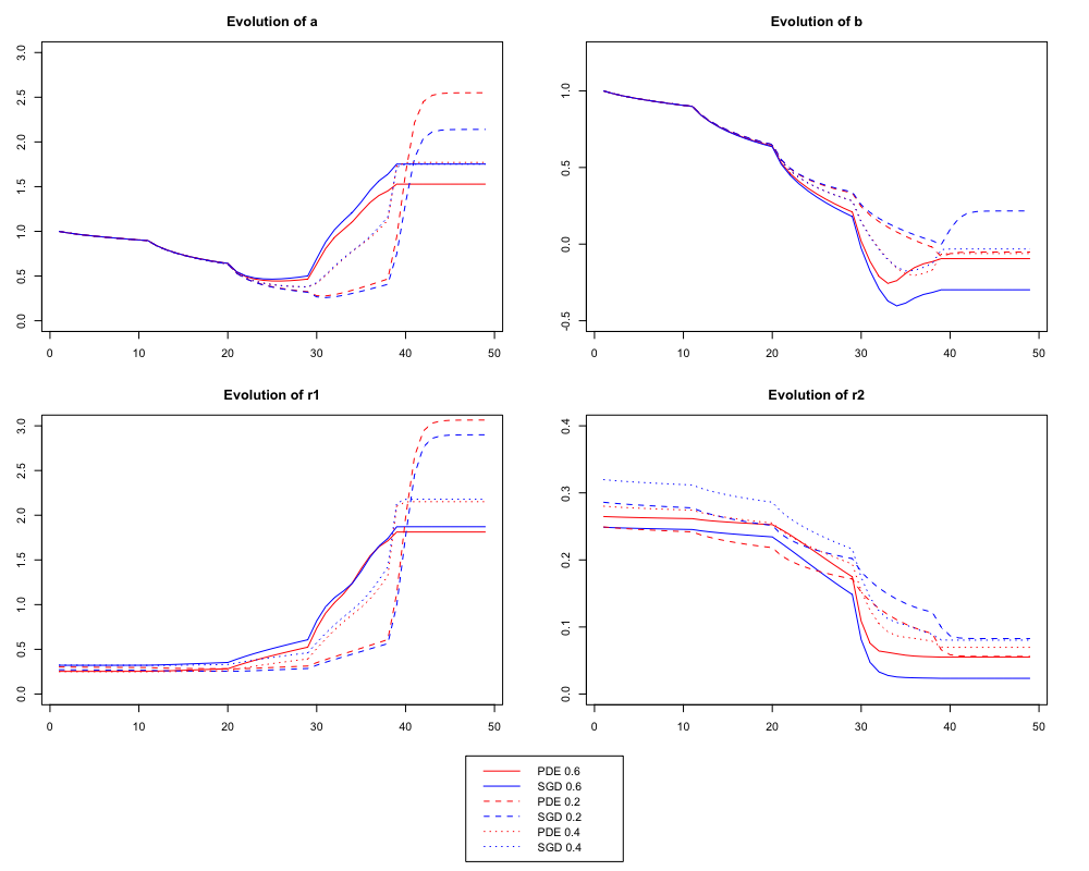
Figure 7: Evolution of four parameters from ReLU activation for SGD and PDE algorithms varying Δ\Delta. The x-axis represents the iteration, where 1-9 represents iterations 1-9, 10-19 represents iterations (10,20,30,40,50,60,70,80,90,100), 20-28 represents iterations (200, 300, 400, 500, 600, 700,800,900,1000), and so on.
Refer to caption

We first look at the closeness of the SGD and PDE under ReLU for the AmFam data to see how well the PDE simulation does for real world data. First, we set d=252d=252, the number of columns in the training set. We then set s=120s=120, N=200N=200, ϵ=2∗10−4\epsilon=2*10^{-4}, ξ(t)=t−1/4\xi(t)=t^{-1/4}, J=100J=100, and each progressive step/iteration of the algorithm to be 1∗10−31*10^{-3}.

Figure 8: Second layer weight distribution observed on two-layer network (250,250) ran on AmFam Data, and weight distributions derived from PDE simulation using Piecewise Linear Activation Function for various choices of weights from second layer.
Refer to caption
Figure 9: Bimodal Nature observed in various layers of three-layer networks run on AmFam Data.
Refer to caption
Figure 10: Bimodal Nature observed in various layers of four-layer networks run on AmFam Data.
Refer to caption

We then create an association matrix Σ\Sigma of all the variables in the train set by taking every 500th data point in the train set and applying the function mixed_\_assoc, which allows us to calculate a pairwise association between all variables in a data-frame. We then subset Σ\Sigma as Σ1=Σ1:s,1:s\Sigma_{1}=\Sigma_{1:s,1:s} and Σ2=Σ(s+1):d,(s+1):d\Sigma_{2}=\Sigma_{(s+1):d,(s+1):d}, i.e. the association matrices of the first ss variables and last d−sd-s variables.

We use the make.positive.definite function to convert each of the Σi\Sigma_{i} into a positive definite matrix Σi+\Sigma_{i}^{+}, and then use the cor2cov function to convert Σi+\Sigma_{i}^{+} into a covariance matrix 𝚺i+{\bm{\Sigma}}_{i}^{+}. We then initialize rj,i​(0)=‖Zj,i‖2r_{j,i}(0)=\|Z_{j,i}\|_{2}, where (Z1,i)i≤N∼i.i.d.N(0,𝚺1+)(Z_{1,i})_{i\leq N}\sim_{i.i.d.}N(0,{\bm{\Sigma}}_{1}^{+}) and (Z2,i)i≤N∼i.i.d.N(0,𝚺2+)(Z_{2,i})_{i\leq N}\sim_{i.i.d.}N(0,{\bm{\Sigma}}_{2}^{+}) indepedently, along with ai​(0)=1a_{i}(0)=1, bi​(0)=1b_{i}(0)=1. We sequentially compute 𝐫i​(t){\bf r}_{i}(t) for 5∗1055*10^{5} iterations.

In Figure 7, for evolution of aa, we compute 1N​∑i=1Nai\frac{1}{N}\sum_{i=1}^{N}a_{i} for the SGD and 1J​∑i=1Jai​(t)\frac{1}{J}\sum_{i=1}^{J}a_{i}(t) for the PDE. We do similar calculates for bb, r1r_{1}, and r2r_{2}. We also vary Δ\Delta to see how the parameters change. For the most part, it appears that there is a good match in the evolutions of the parameters between the SDG and PDE across varying Δ\Delta.

We next look at the weight distributions produced from the PDE. We first fit a simple neural network with two hidden layers, each layer containing 250 nodes to the AmFam data. We focus our attention on the weights from the second layer. In Figure 8, we see the top left figure is the density of the weights produced from the 2nd layer. The top right is sampling 250 of the weights produced from the second layer and running them through the PDE simulation using the Piecewise Linear Activation Function. The bottom two are looking at the means of weights from the 250 nodes (either averaging across weights coming from the same node or going to the same node) and running them through the PDE simulation using the Piecewise Linear Activation Function. It looks like while in the original 2 layer density it is centered around 0 and seems relatively unimodal, in the other 3 density plots, there is a tendency towards a bimodal density distribution.

We also found that the bimodalness arises in weight distributions of different layers in various neural networks run on the AmFam data, as shown in Figures 10 and 10.

4.5.2 Theoretical

In addition to seeing how the PDE affects the AmFam data, we also try to create a “true” theoretical distribution through simulation. To do this, we will use the interpolation activation function with s1=−2.5s_{1}=-2.5, s2=7.5s_{2}=7.5, t1=0.5t_{1}=0.5, t2=1.5t_{2}=1.5, J=100J=100, N=2000N=2000, Δ=0.8\Delta=0.8, and d=250d=250, with an increment size of 1∗10−51*10^{-5} and ξ⁡(t)=1\xi(t)=1.

We create a target vector yy of size NN, where yi=1y_{i}=1 with probability 1/21/2 and 00 with probability 1/21/2. Next, we create our covariance matrix, 𝚺{\bm{\Sigma}} of size dd by dd, where the diagonal entries are (1+Δ)2(1+\Delta)^{2} and the off diagonals are 0.0010.001. We then sample x∼N⁡(0,𝚺)x\sim N(0,{\bf\Sigma}). We next create 𝚺2{\bf\Sigma}_{2} of size dd by dd, where the diagonal entries are (Δ2/d)(\Delta^{2}/d), and the off diagonals are 0.0010.001. We then initialize ri​(0)=‖Zi‖2r_{i}(0)=\|Z_{i}\|_{2}, where (Zi)i≤J∼i.i.d.N(0,𝚺2)(Z_{i})_{i\leq J}\sim_{i.i.d.}N(0,{\bf\Sigma}_{2}). We sequentially compute the value of 𝐫⁡(t){\bf r}(t) using 𝐫(t+δt)≈𝐫(t)−Jξ(t)∇R¯∞,J(𝐫(t))δt{\bf r}(t+\delta t)\approx{\bf r}(t)-J\xi(t)\nabla{\bar{R}}_{\infty,J}({\bf r}(t))\delta t from Section 4.4.1.

Once we have run 𝐫⁡(t){\bf r}(t) through the PDE approximation, we then set them as the initial weights in a standard neural network in RR using the neuralnet package, with a single hidden layer of 100 nodes and then two hidden layers, each with 100 nodes. Using yy and xx initialized from above, we run the two neural networks and extract the weights from the output layer.

We then set these extracted weights as 𝐫⁡(0){\bf r}(0) and run them through the PDE approximation. We observe the transformation of 𝐫⁡(t){\bf r}(t) in Figure 11 and the weight distributions produced from the single hidden layer neural network and two hidden layer neural network after running the extracted weights through the PDE approximation in Figure 12.
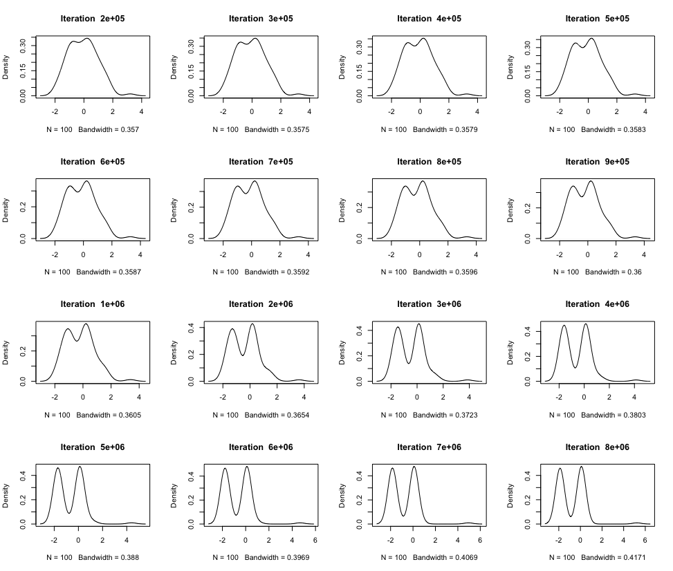
Figure 11: Evolution of weight distribution under PDE approximation with 𝐫⁡(0){\bf r}(0) taken from extracted weights of single hidden layer neural network with 100 nodes.
Refer to caption
Figure 12: Weight Distributions after running PDE approximation on extracted weights from neural networks with one hidden layer of 100 nodes and two hidden layers of 100 nodes each, respectively.
Refer to caption

4.6 Analysis of Distribution of Weights

To compare the distributions produced from neural networks on the AmFam data to the theoretical distributions produced from the PDE approximation, we utilize two classical distribution distance metrics, the Kullback-Leibler divergence (KL) and L1 distance. The PDE approximation provides theoretical mathematical models to analyze the bimodality phenomenon, and we want to see which fit neural networks get closest to/achieve that bimodal phenonemon. Iterating through each of the neural networks trained on the AmFam data, we compute the KL and L1 distance measures using the “true” theoreticals produced from the PDE approximation as the base distribution (we will refer to distribution A as the true theoretical that utilized a single hidden layer of 100 nodes, and distribution B as the other). Once the KL distances are computed for the two distributions, we will rank them from lowest to highest with respect to distribution A and distribution B, and then average their rankings. This averaged rank is stored in the variable kl.avg, and the same is done for the L1 distances, their average being stored in the variable l1.avg.
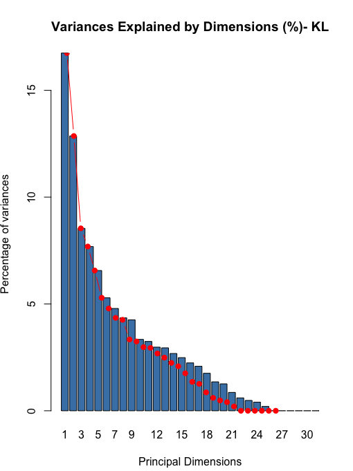
Figure 13: Variance explained from MCA.
Refer to caption
Figure 14: MCA Analysis plotted with KL divergence variable.
Refer to caption
Figure 15: MCA Analysis plotted with L1 distance variable.
Refer to caption

Multiple Correspondence Analysis (MCA) is a generalization of principal component analysis when the variables to be analyzed are mainly categorical instead of quantitative. It allows us to identify which attributes of the neural network contribute the most to reducing the distance metrics. In Figures 15 and 15, we produce plots from the MCA based on a reduction to the first two dimensions/components. On these plots, we also graph the KL divergence and L1 distance variables based on their values of the first two dimensions/components produced from the MCA. Looking at the factor maps, the red dots represent variables, while the blue dots represent the individual neural networks. By plotting the kl.avg and l1.avg variables on the factor map, we can roughly see which neural networks and attributes achieve the lower values of those variables.

Using a weighted average based on dimension contribution from the first five dimensions (seen in Figure 13), we find that for both of the KL and L1 distance variables, the MCA suggests that a three layer network with Layer 1 around 100-150 nodes, Layer 2 around 25-50 nodes, and Layer 3 around 25 nodes with the Rectifier activation, mini batch of 100, and max w2 of 25 seems to do best, with the second layer having the distribution most similar to distribution A and distribution B.

References

  • [1] Dariusz Buraczewski, Ewa Damek, Thomas Mikosch, Stochastic Models with Power-Law Tails: The Equation X=AX+B, Springer Series in Operations Research and Financial Engineering, 2016. ISSN 1431-8598. doi 10.1007/978-3-319-29679-1.
  • [2] Dariusz Buraczewski, Jeffrey F. Collamore, Ewa Damek, and Jacek Zienkiewicz, Large Deviation Estimates for Exceedance Times of Perpetuity Sequences and their Dual Processes, The Annals of Probability, 2014, doi 10.1214/15-AOP1059.
  • [3] Ian Goodfellow, Yoshua Bengio, and Aaron Courville. Deep Learning. The MIT Press, 2016.
  • [4] Hoeffding, Wassily, A Non-Parametric Test of Independence, The Annals of Mathematical Statistics, Vol. 19, No. 4 (Dec., 1948), pp. 546-557.
  • [5] Hollander, M. and Wolfe, D.A., Nonparametric Statistical Methods, John Wiley and Sons, New York, 1973.
  • [6] Kevei, Peter, Implicit Renewal Theory in the Arithmetic Case, Journal of Applied Probability, 2016, doi 10.1017/jpr.2017.31.
  • [7] Victor Luo and Yazhen Wang. How many factors influence minima in SGD? arXiv:2009.11858, 2020.
  • [8] Mentemeier,Sebastian and Wintenberger, Olivier , Asymptotic Independence ex machina – Extreme Value Theory for the Diagonal BEKK-ARCH(1) Model, arXiv:1907.10379v1 [math.PR], 2019.
  • [9] Song Mei, Andrea Montanari, Phan-Minh Nguyen, A Mean Field View of the Landscape of Two-Layer Neural Networks, Proceedings of the National Academy of Sciences, 2018. ISSN 0027-8424. doi: 10.1073/pnas.1806579115.
  • [10] Sznitman, Alain-Sol, Topics in propagation of chaos, Ecole d’ete de probabilites de Saint-Flour XIX - 1989, pp. 165-251. Spring, 1991.
  • [11] Yazhen Wang and Shang Wu. Asymptotic analysis via stochastic differential equations of gradient descent algorithms in statistical and computational paradigms. Journal of Machine Learning Research 21(199):1-103, 2020.