The standard paradigm of cosmology, $\Lambda$CDM plus inflationary cosmology [1, 2, 3, 4, 5, 6, 7], matches all known experimental data (after suitable fitting of the parameters coming from specific models) and solves all problems: specifically the CMBR fluctuation data can be fitted, the standard pre-inflationary Hot Big Bang cosmology problems can be solved [5, 6, 7], and one can generate the Standard Model particles by a model of reheating.

However, the models of holographic cosmology, based on the application of the AdS/CFT correspondence [8] (see the books [9, 10] for more information) to 3+1 dimensional cosmological backgrounds, specifically the general phenomenological model of McFadden and Skenderis, defined in [11, 12], were shown to also fit the same CMBR data and solve the same problems. Specifically, in [13, 14] it was shown that one can make a fit of the phenomenological model to the CMBR data with the same number of parameters, that is within 0.5 in $\chi^{2}$ from the standard $\Lambda$CDM plus inflation fit (840.0 for holographic cosmology vs. 823.5 for $\Lambda$CDM, see table V in [14]), thus being experimentally indistinguishable from the latter. Further, in [15, 16] it was shown that the usual problems of Hot Big Bang cosmology also also solved by the holographic cosmology models, and in [17] a model of reheating was proposed.

However, while the smoothness and horizon problem, entropy problem, perturbations problem and baryon asymmetry problem were solved generically, and for the flatness problem the condition on a combination of the parameters, $f_{1}<0$, necessary to have a relevant energy-momentum tensor $T_{ij}$ that solves the problem, has a concrete solution, solved on most of the parameter space, for the monopole problem only a toy field theory model was analyzed, and shown to solve the problem. In this letter we show that we can extend the proof from the toy model to the whole set of purely bosonic phenomenological models, first reviewing the solution of the monopole problem by having an electric global symmetry current that is an irrelevant operator, then showing how this can be in the generic model.

First, we quickly review the solution of the monopole problem, based on the fact that the electric current $j_{\mu}^{a}$ is an irrelevant operator (which was found to be true in the toy model analyzed in [15, 16]).

The monopole problem is the following. Considering an expanding Universe, with an expanding horizon size, undergoing a phase transition, like a Grand Unified Theory (GUT) phase transition. Then the Kibble mechanism guarantees that one creates about one monopole per nucleon. The Kibble mechanism refers to the fact that, when the temperature drops and the scalar takes a VEV in the vacuum, thus breaking the symmetry, it takes a random value for each causally connected patch. Then when taking a few patches, one generically has a larger patch with monopole topology for the scalar (thus also for the gauge fields), thus creating a monopole per region of the order of the horizon. When nucleons are formed, a similar mechanism creates one nucleon per horizon, therefore leading to one monopole per nucleon.

Yet experimentally, direct searches for monopoles on Earth finds less than $10^{-30}$ monopoles per nucleon [18] (see also [19], chapter 4.1.C), so one needs a mechanism to dilute them.

In the holographic cosmology model, gauge field perturbations $A_{\mu}^{a}$ in the bulk cosmology correspond to global non-Abelian symmetry currents $j_{\mu}^{a}$ in field theory, and (’t Hooft-Polyakov) monopole configurations in the bulk correspond to vortex configurations on the boundary. Dilution of monopoles as cosmological time goes forward corresponds to dilution of the vortex current along the inverse RG flow, i.e., towards the UV. Considering the two-point function $\langle\tilde{j}_{\mu}^{a}(p)\tilde{j}_{\nu}^{b}(-p)\rangle\propto p^{1+2\delta}$, we find that we need the vortex current $\tilde{j}_{\mu}^{a}(p)$ to be a (marginally) relevant operator, $\delta(\tilde{j})>0$.

But for conformal theories [20, 21] and, by extension, to generalized conformal theories, the two-point function of the electric currents $j_{\mu}^{a}$, constrained to be of the form

$$\langle j_{\mu}^{a}(p)j_{\nu}^{b}(-p)\rangle=\sqrt{p^{2}}\left(\delta_{\mu\nu}-\frac{p_{\mu}p_{\nu}}{p^{2}}\right)K^{ab}\;,$$

(2.1)

implies that the S-dual vortex currents have an inverse $K^{ab}$,

$$\langle\tilde{j}_{\mu}^{a}(p)\tilde{j}_{\nu}^{b}(-p)\rangle=\sqrt{p^{2}}\left(\delta_{\mu\nu}-\frac{p_{\mu}p_{\nu}}{p^{2}}\right)K^{-1}_{ab}\;,$$

(2.2)

so in effect an inverse anomalous dimension, $\delta(j)=-\delta(\tilde{j})$. In other words, the need for a (marginally) relevant vortex current $\tilde{j}_{\mu}^{a}$ implies the need for a (marginally) irrelevant electric current $j_{\mu}^{a}$.

Finally, in [15, 16] it was noted that one has to check that a vortex solution does exist, so that the vortex current exists also. Yet, since the ’t Hooft-Polyakov monopole in the bulk would be dual to a non-Abelian vortex in field theory, and such non-Abelian vortices were found only in complicated theories, not relevant for the phenomenological action, with all the fields in the adjoint of $SU(N)$, Dirac monopoles (singular, point-like) were considered instead in the bulk, corresponding in the field theory on the boundary to what was dubbed ”Dirac vortices”, namely singular, point-like versions of the vortices. The toy model considered in [15, 16] admitted such solutions, so there exist models within the phenomenological class with vortex solutions. Since we will deal with the whole phenomenological class, and the existence of cosmological monopoles, thus of field theory vortices, must be imposed on any consistent model, it is enough to know that such models exist.

In this section, we will review the general points of the calculation of the electric current two-point function in [15, 16]), and point out that they apply to any model in the phenomenological class that has a global symmetry current.

The phenomenological class, written in the form with 4-dimensional dimensions for the fields, has an Euclidean action for one gauge field $A_{\mu}$ and scalar $\Phi^{M}$ and fermion $\psi^{L}$ fields in the adjoint of $SU(N)$, given by

	$\displaystyle S_{\rm QFT}$	$\displaystyle=$	$\displaystyle\frac{1}{g^{2}_{YM}}\int d^{3}x\mathop{\rm Tr}\nolimits\left[\frac{1}{2}F_{ij}F^{ij}+\delta_{M_{1}M_{2}}D_{i}\Phi^{M_{1}}D^{i}\Phi^{M_{2}}+2\delta_{L_{1}L_{2}}\bar{\psi}^{L_{1}}\gamma^{i}D_{i}\psi^{L_{2}}\right.$		(3.1)
			$\displaystyle\left.+\sqrt{2}\mu_{ML_{1}L_{2}}\Phi^{M}\bar{\psi}^{L_{1}}\psi^{L_{2}}+\frac{1}{6}\lambda_{M_{1}...M_{4}}\Phi^{M_{1}}...\Phi^{M_{4}}\right]\;,$		(3.2)

plus a nonminimal coupling of gravity to the scalar $1/(2g^{2}_{YM})\int\xi_{M}R(\Phi^{M})^{2}$. It has dimensionless couplings, except $g^{2}_{YM}$, which appears in the quantum theory only in the effective coupling combination $g^{2}_{\rm eff}=\frac{g^{2}N}{q}$, and the fields have $[A_{i}]=1=[\Phi^{M}]$ and $[\psi^{L}]=3/2$. Moreover, we will only consider the case without fermions, so $\psi^{L}=0$, and the dimensionless couplings are $\lambda_{M_{1}...M_{4}},\xi_{M}$. However, $\xi_{M}$ only is relevant to the energy-momentum tensor (since otherwise the corresponding term is zero in a flat background), so the only relevant dimensionless couplings for our calculation are $\lambda_{M_{1}...M_{4}}$. The model is super-renormalizable, and has generalized conformal symmetry, meaning that the only dimensionful coupling is $g_{YM}$.

Since we have not selected a model with a certain global symmetry within the phenomenological class, we cannot write an explicit expression for the global current $j_{\mu}^{a}$, as in [15, 16]), but we assume that one exists.

To prove that the electric current $j_{\mu}^{a}$ is a (marginally) irrelevant operator, we need to calculate its two-point function $\langle j_{\mu}^{a}(p)j_{\nu}^{b}(-p)\rangle$, specifically the finite one-loop result (giving the normalization) and the divergent part of the two-loop diagrams (giving the anomalous dimension). At one-loop, there is one Feynman diagram for the two-point function, and Feynman diagrams for the renormalization, both given in Fig.1. At two-loops, there are Feynman diagrams with and without external gauge field insertions, in Fig.2.

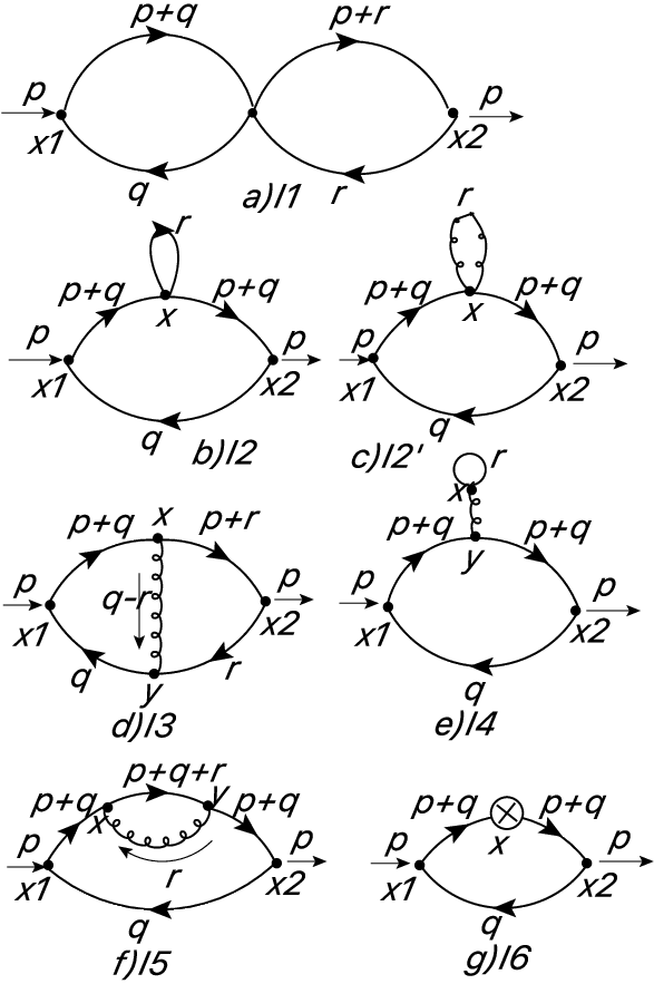
Ignoring the $SU(N)$ indices (which are all taken care of by ’t Hooft’s double-line notation, as replacing $g^{2}_{YM}$ with the effective $g^{2}_{\rm eff}=g^{2}N/q$), the fields of the toy model in [15, 16] were $\phi_{i}^{a}$ and $A_{\mu}$, with 4-point scalar vertices

$$-\lambda(2\pi)^{3}\delta^{3}(k_{1}+k_{2}+k_{3}+k_{4})\epsilon^{abe}\epsilon_{cde}=-2\lambda\delta_{ab}^{cd}(2\pi)^{3}\delta^{3}(k_{1}+k_{2}+k_{3}+k_{4}).$$

(3.3)

and 3-point $\phi\phi A$ and 4-point $\phi\phi AA$, as well as pure gluonic ones, completely determined by minimal coupling (gauge invariance). Moreover, by explicit calculation of the Feynman diagrams, one finds that $I_{1}=I_{2a}=I_{2b}=I_{4}=0$, while the counterterm diagram $I_{6}$ is finite and multiplied by $\lambda_{\rm ct}$, and since the one-loop result is finite, and moreover the theory itself is one-loop finite, so $I_{6}$ is irrelevant to the calculation as well.

When looking at the calculation of these vanishing integrals, it is easy to see that $I_{1},I_{2a},I_{2b},I_{4}$ vanishing is unrelated to the form of the vertices: in the case of $I_{1}$, the 4-point scalar vertex contribution is an overall factor, while for $I_{2a},I_{2b},I_{4}$ the vanishing comes from the factorized loop. Also, the fact that $I_{6}$ is finite is again a result of the fact that it has the topology of the one-loop result. So for a generic theory, we are still left with only the diagrams $I_{3},I_{5},I_{7a},I_{7b},I_{8}$. But in these diagrams, since the propagators are still Klein-Gordon (for the scalars and for the gauge field, in the Feynman gauge) times delta functions for indices, and the relevant vertices are $\phi\phi A$ vertices completely determined by minimal coupling, it is easy to check that the expressions for the Feynman diagrams are the same ones written and calculated in [15, 16]. The only thing different is an overall factor equal to the number of scalars running in the original scalar loop, but since this factor equals the same extra factor at one-loop, this becomes an overall factor in the two-point function, and does not change the value of the two-loop anomalous dimension. That means that we still have, for a generic theory,

$$\delta(j)=\frac{2}{\pi^{2}}g^{2}_{\rm eff}>0\;,$$

(3.4)

that is, an irrelevant operator, as we wanted. Therefore, the dual (vortex) current has $\delta(\tilde{j})=-\delta(j)<0$, so the vortices and holographic dual monopoles get diluted, as we wanted.

In this letter we have removed a caveat from the previous analysis of the problems with Hot Big Bang cosmology within holographic cosmology, showing that the monopole problem is not solved only for some toy models, but generically, for any purely bosonic model within the phenomenological class. In terms of matching experimental data and solving theoretical problems, this means that the holographic cosmology paradigm is as good as the usual, $\Lambda$CDM plus inflation, paradigm. This should not be a surprise, since the two are related by changing the strength of the coupling (inflation means a perturbative gravitational theory, holographic cosmology a perturbative 3-dimensional field theory).

Acknowledgements

The work of UP is supported in part by FAPESP grant 2018/22008-7. The work of HN is supported in part by CNPq grant 301491/2019-4 and FAPESP grants 2019/21281-4 and 2019/13231-7. HN would also like to thank the ICTP-SAIFR for their support through FAPESP grant 2016/01343-7.

References

- [1] R. Brout, F. Englert, and E. Gunzig, “The Creation of the Universe as a Quantum Phenomenon,” Annals Phys. 115 (1978) 78.
- [2] A. A. Starobinsky, “Spectrum of relict gravitational radiation and the early state of the universe,” JETP Lett. 30 (1979) 682–685.
- [3] A. A. Starobinsky, “A New Type of Isotropic Cosmological Models Without Singularity,” Adv. Ser. Astrophys. Cosmol. 3 (1987) 130–133.
- [4] K. Sato, “First Order Phase Transition of a Vacuum and Expansion of the Universe,” Mon. Not. Roy. Astron. Soc. 195 (1981) 467–479.
- [5] A. H. Guth, “The Inflationary Universe: A Possible Solution to the Horizon and Flatness Problems,” Phys. Rev. D23 (1981) 347–356. [Adv. Ser. Astrophys. Cosmol.3,139(1987)].
- [6] A. D. Linde, “A New Inflationary Universe Scenario: A Possible Solution of the Horizon, Flatness, Homogeneity, Isotropy and Primordial Monopole Problems,” Phys. Lett. 108B (1982) 389–393. [Adv. Ser. Astrophys. Cosmol.3,149(1987)].
- [7] A. Albrecht and P. J. Steinhardt, “Cosmology for Grand Unified Theories with Radiatively Induced Symmetry Breaking,” Phys. Rev. Lett. 48 (1982) 1220–1223. [Adv. Ser. Astrophys. Cosmol.3,158(1987)].
- [8] J. M. Maldacena, “The Large N limit of superconformal field theories and supergravity,” Int. J. Theor. Phys. 38 (1999) 1113–1133, arXiv:hep-th/9711200 [hep-th]. [Adv. Theor. Math. Phys.2,231(1998)].
- [9] H. Nastase, Introduction to the ADS/CFT Correspondence. Cambridge University Press, Cambridge, 2015.
- [10] M. Ammon and J. Erdmenger, Gauge/gravity duality. Cambridge University Press, Cambridge, 2015.
- [11] P. McFadden and K. Skenderis, “Holography for Cosmology,” Phys. Rev. D81 (2010) 021301, arXiv:0907.5542 [hep-th].
- [12] P. McFadden and K. Skenderis, “The Holographic Universe,” J. Phys. Conf. Ser. 222 (2010) 012007, arXiv:1001.2007 [hep-th].
- [13] N. Afshordi, C. Coriano, L. Delle Rose, E. Gould, and K. Skenderis, “From Planck data to Planck era: Observational tests of Holographic Cosmology,” Phys. Rev. Lett. 118 (2017) no. 4, 041301, arXiv:1607.04878 [astro-ph.CO].
- [14] N. Afshordi, E. Gould, and K. Skenderis, “Constraining holographic cosmology using Planck data,” Phys. Rev. D95 (2017) no. 12, 123505, arXiv:1703.05385 [astro-ph.CO].
- [15] H. Nastase and K. Skenderis, “Holography for the very early Universe and the classic puzzles of Hot Big Bang cosmology,” Phys. Rev. D 101 (2020) no. 2, 021901, arXiv:1904.05821 [hep-th].
- [16] H. Nastase, “Holographic cosmology solutions of problems with pre-inflationary cosmology,” JHEP 12 (2020) 026, arXiv:2008.05630 [hep-th].
- [17] H. Nastase, “Reheating in holographic cosmology and connecting to -MSSM constructions for particle physics,” arXiv:2008.06144 [hep-th].
- [18] Y. Zeldovich and M. Khlopov, “On the Concentration of Relic Magnetic Monopoles in the Universe,” Phys. Lett. B 79 (1978) 239–241.
- [19] S. Weinberg, Cosmology. 2008.
- [20] E. Witten, “SL(2,Z) action on three-dimensional conformal field theories with Abelian symmetry,” arXiv:hep-th/0307041 [hep-th].
- [21] C. P. Herzog, P. Kovtun, S. Sachdev, and D. T. Son, “Quantum critical transport, duality, and M-theory,” Phys. Rev. D75 (2007) 085020, arXiv:hep-th/0701036 [hep-th].