跳到论文正文
W Papers独立论文阅读器 arXiv:2012.14737 论文正文 计算阅读时间 · 0%
引用这篇论文根据当前论文元数据生成,正式投稿前建议核对。


License: arXiv.org perpetual non-exclusive license
arXiv:2012.14737v1 [gr-qc] 29 Dec 2020

Quantum Entanglement and Thermodynamics of Boson-Antiboson Pair Creation Modes in the Noncommutative Bianchi I Universe

M. F. Ghiti1,2    N. Mebarki2 and H. Aissaoui2 Address: 1. Ecole Normale Supérieure (ENSC), Assia Djebar, Constantine, Algeria
2. Laboratoire de Physique Mathématique et Subatomique (LPMS),
Constantine 1 University, Constantine, Algeria
farouk.ghiti@yahoo.com
Abstract

Within the quantum field theory approach and using the technique of Bogoliubov transformations, the von Neumann boson-antiboson pair creation quantum entanglement entropy is studied in the context of the noncommutative Bianchi I universe. It is shown that the latter have a behavior depending strongly on the choice of the noncommutativity θ\theta parameter, k⟂k_{\perp}-frequency modes and the structure of the curved spacetime. Moreover, the relationship between the Bose-Einstein condensation and quantum entanglement is also discussed.

keywords
Noncommutative Bianchi I universe, Pair creation, Boson-Antiboson quantum entanglement entropy, Quantum information, Bose-Einstein Condensation
PACS
PACS numbers: 03.65.Ud, , 03.65.-w, 03.67.-a, 03.75.Nt, 04.62.+v

1 Introduction

During the last few years, The quantum entanglement (Q.E.) phenomenon has been of great interest for many people in the field of quantum information in both flat and curved spacetime [1, 2, 3, 4, 5, 6, 7, 8, 9, 10, 11, 12, 13, 14]. Moreover, it turns out that the pair creation process is intimately related to the quantum entanglement and strongly depends on the nature of the particles as well as on the structure of the spacetime [5, 9, 11, 15, 16]. Furthermore, as a possible scenario to explain dark matter and dark energy as well as the anisotropies found in the cosmic microwave background (C.M.B.), is the noncommutative geometry (N.C.G) [17, 18, 19, 20, 21, 22]. In fact, many models have been proposed so far where it has been shown that the noncommutativity θ\theta-parameter plays an important role [23, 24, 25, 26, 27, 28, 29, 30, 31, 32]. The goal of this paper is to study the process of creating boson-antiboson pairs in the noncommutative (N.C.) Bianchi I universe and show its relationship with quantum entanglement and Bose-Einstein condensation (B.E.C.) phenomena. The role played by the spacetime noncommutativity is also emphasized. In section 2, we present the necessary mathematical formalism. Section 3 contains our numerical results and discussions. Finally, in section 4, we draw our conclusions.

2 Mathematical Formalism

The N.C. spacetime is characterized by the coordinates operators x^μ\hat{x}^{\mu} (μ=0,3¯)(\mu=\overline{0,3}) satisfying the following commutation relation:

[x^μ,x^ν]=i​θμ​ν\left[\hat{x}^{\mu},\hat{x}^{\nu}\right]=i\,\theta^{\mu\nu} (1)

where θμ​ν\theta^{\mu\nu} are antisymmetric matrix elements which control the noncommutativity of the spacetime. The N.C. matter scalar density of the massless Seiberg-Witten (S.W.) bosonic field φ^\hat{\varphi} reads :

ℒ=e^∗(g^μ​ν∗(D^μ​φ^)†∗D^ν​φ^)\mathcal{L}=\hat{e}\ast\left(\hat{g}^{\mu\nu}\ast\left(\hat{D}_{\mu}\hat{\varphi}\right)^{\dagger}\ast\hat{D}_{\nu}\hat{\varphi}\right) (2)

here, the deformed tetrad is given by :

e^=d​e​t∗​(e^μa)=14!​ϵμ​ν​ρ​σ​ϵa​b​c​d​e^μa∗e^νb∗e^ρc∗e^σd\hat{e}=det_{\ast}\left(\hat{e}^{a}_{\mu}\right)=\frac{1}{4!}\epsilon^{\mu\nu\rho\sigma}\epsilon_{a\,b\,c\,d}\,\hat{e}^{a}_{\mu}\ast\hat{e}^{b}_{\nu}\ast\hat{e}^{c}_{\rho}\ast\hat{e}^{d}_{\sigma} (3)

where ϵμ​ν​ρ​σ\epsilon^{\mu\nu\rho\sigma} and ϵa​b​c​d\epsilon_{a\,b\,c\,d} are the completely antisymmetric tensors in curved and flat spacetime respectively. The gauge covariant derivative is given by : D^μφ^=(∂μ−ieA^μ)∗φ^\hat{D}_{\mu}\hat{\varphi}=\left(\partial_{\mu}-ie\hat{A}_{\mu}\right)\ast\hat{\varphi}. The corresponding Klein-Gordon equation is shown to take the following form (See Appendix A) :

(gμ​ν∂μ∂ν−1−g∂μ(−ggμ​ν)∂ν)φ^−i2​−gθα​β∂μ(∂α+−g∂βgμ​ν∂νφ^)+\displaystyle\left(g^{\mu\nu}\partial_{\mu}\partial_{\nu}-\frac{1}{\sqrt{-g}}\partial_{\mu}\left(\sqrt{-g}g^{\mu\nu}\right)\partial_{\nu}\right)\hat{\varphi}-\frac{i}{2\sqrt{-g}}\theta^{\alpha\beta}\partial_{\mu}\left(\partial_{\alpha}+\sqrt{-g}\partial_{\beta}g^{\mu\nu}\partial_{\nu}\hat{\varphi}\right)+
18​−g​θα​β​∂μ(∂α∂ρ(−g​gμ​ν)​∂β∂σ∂νφ^+∂ρ(∂α−g​∂βgμ​ν​∂σ∂νφ^)+CLOSE\displaystyle\frac{1}{8\sqrt{-g}}\theta^{\alpha\beta}\partial_{\mu}\left(\partial_{\alpha}\partial_{\rho}\left(\sqrt{-g}g^{\mu\nu}\right)\partial_{\beta}\partial_{\sigma}\partial_{\nu}\hat{\varphi}+\partial_{\rho}\left(\partial_{\alpha}\sqrt{-g}\partial_{\beta}g^{\mu\nu}\partial_{\sigma}\partial_{\nu}\hat{\varphi}\right)+\right.
OPEN∂α∂ρ−g​∂β∂σgμ​ν​∂νφ^)+i2​−g​θα​β​∂μ(∂α(−g​gμ​ν)​∂β∂νφ^)=0\displaystyle\left.\partial_{\alpha}\partial_{\rho}\sqrt{-g}\partial_{\beta}\partial_{\sigma}g^{\mu\nu}\partial_{\nu}\hat{\varphi}\right)+\frac{i}{2\sqrt{-g}}\theta^{\alpha\beta}\partial_{\mu}\left(\partial_{\alpha}\left(\sqrt{-g}g^{\mu\nu}\right)\partial_{\beta}\partial_{\nu}\hat{\varphi}\right)=0 (4)

where gg is the determinant of the metric. In what follows, using dimensionless spacetime coordinates (t,x,y,z)(t,x,y,z), we consider a Bianchi I universe where the metric has the form:

d​s2=−d​t2+t2​(d​x2+d​y2)+d​z2ds^{2}=-dt^{2}+t^{2}\left(dx^{2}+dy^{2}\right)+dz^{2} (5)

(here the time tt is related to the cosmological parameters of the model). By convention, we choose the spacetime signature as being (−,+,+,+)(-,+,+,+) and for simplicity, we take :

θμ​ν=[00θ00000−θ0000000]\theta_{\mu\nu}=\left[\begin{array}[]{cccc}0&0&\theta&0\\ 0&0&0&0\\ -\theta&0&0&0\\ 0&0&0&0\end{array}\right] (6)

(notice that the choice of the θμ​ν\theta^{\mu\nu} does not affect so much our conclusions). Using Maple 16 tensor package, the non-vanishing components of the vierbeins up to O⁡(θ2)O\left(\theta^{2}\right) have the following expressions:

e^00~\displaystyle\hat{e}^{\tilde{0}}_{0} =\displaystyle= e^33~=1\displaystyle\hat{e}^{\tilde{3}}_{3}=1
e^11~\displaystyle\hat{e}^{\tilde{1}}_{1} =\displaystyle= e^22~=1t​(1−25​θ2128)\displaystyle\hat{e}^{\tilde{2}}_{2}=\frac{1}{t}\Big(1-\frac{25\,\theta^{2}}{128}\Big) (7)

and therefore, the corresponding deformed Bianchi I metric up to O⁡(θ2)O\left(\theta^{2}\right) is given by:

d​s2=−d​t2+t2​(1−2164​θ2)​(d​x2+d​y2)+d​z2ds^{2}=-dt^{2}+t^{2}\left(1-\frac{21}{64}\theta^{2}\right)\left(dx^{2}+dy^{2}\right)+dz^{2} (8)

It is worth mentioning, as pointed out in references [5, 29, 33, 34, 35] that since the metric presents a space-like singularity at t=0t=0, it is difficult to define the particle state within the adiabatic approach. To do so, we first follow a quasiclassical approach of Ref. [34] to identify the positive and negative frequency modes and look for the asymptotic behavior of the solutions at t→0t\rightarrow 0 and t→∞t\rightarrow\infty. Secondly, we solve the N.C. Klein Gordon equation and compare the solutions with the above quasiclassical limit. After straightforward but lengthy calculations, Eq. (2) is simplified to

(1+i​θt​∂~2−θ24​t2​∂~22)​∂~02​φ^+\displaystyle\left(1+\frac{i\theta}{t}\tilde{\partial}_{2}-\frac{\theta^{2}}{4t^{2}}\tilde{\partial}_{2}^{2}\right)\tilde{\partial}_{0}^{2}\hat{\varphi}+ 2t​(1+i​θ2​t​∂~2)​∂~0​φ^+(1t2​(1+2164​θ2)​(∂~12+∂~22)+CLOSE\displaystyle\frac{2}{t}\left(1+\frac{i\theta}{2t}\tilde{\partial}_{2}\right)\tilde{\partial}_{0}\hat{\varphi}+\left(\frac{1}{t^{2}}\left(1+\frac{21}{64}\theta^{2}\right)\left(\tilde{\partial}_{1}^{2}+\tilde{\partial}_{2}^{2}\right)+\right. (9)
OPEN(1+i​θt​∂~2−θ24​t2​∂~22)​∂~32)​φ^=0\displaystyle\left.\left(1+\frac{i\theta}{t}\tilde{\partial}_{2}-\frac{\theta^{2}}{4t^{2}}\tilde{\partial}_{2}^{2}\right)\tilde{\partial}_{3}^{2}\right)\hat{\varphi}=0

here, the tilde stands for a curved spacetime index. To simplify this equation, we set:

φ^=t^−1​f​(t)​h​(t)​exp⁡[i⁡(kx​x+ky​y+kz​z)]\hat{\varphi}=\hat{t}^{-1}f\left(t\right)h\left(t\right)\exp[i\left(k_{x}x+k_{y}y+k_{z}z\right)] (10)

where

t^=t−θ2​ky,f⁡(t)=exp⁡(−θ2​t​ky)\hat{t}=t-\frac{\theta}{2}k_{y},\qquad f\left(t\right)=\exp\left(-\frac{\theta}{2t}k_{y}\right) (11)

where h⁡(t)h\left(t\right) is some regular function. After straightforward but tedious calculations Eq. (9) becomes:

(d2d​t2+k⟂2+2164​θ2​k⟂2t2+kz2)​h​(t)=0\left(\frac{d^{2}}{dt^{2}}+\frac{{k^{2}_{\perp}}+\frac{21}{64}\theta^{2}{k^{2}_{\perp}}}{t^{2}}+k^{2}_{z}\right)h\left(t\right)=0 (12)

where k⟂k_{\perp} is given by:

k⟂2=kx2+ky2k^{2}_{\perp}=k^{2}_{x}+k^{2}_{y} (13)

Now, we adopt the following change of variables :

h⁡(t)=ρμθ+12​exp⁡(−ρ2)​y​(ρ)\displaystyle h\left(t\right)=\rho^{\mu_{\theta}+\frac{1}{2}}\exp\left({-\frac{\rho}{2}}\right)y\left(\rho\right) (14a)
ρ=−2​i​kz​t\displaystyle\rho=-2ik_{z}t (14b)
μθ=i​−14+k⟂2+2164​θ2​k⟂2\displaystyle\mu_{\theta}=i\sqrt{-\frac{1}{4}+k^{2}_{\perp}+\frac{21}{64}\theta^{2}k^{2}_{\perp}} (14c)

Notice that after direct calculations, Eq.(12) takes the following form:

(ρ​d2d​ρ2+(2​μθ+1−ρ)​dd​ρ−(μθ+12))​y​(ρ)=0\left(\rho\frac{d^{2}}{d\rho^{2}}+\left(2\mu_{\theta}+1-\rho\right)\frac{d}{d\rho}-\left(\mu_{\theta}+\frac{1}{2}\right)\right)y\left(\rho\right)=0 (15)

It is important to mention that Eq. (15) has the form of the Kummer’s differential equation [5, 36] :

(ρ​d2d​ρ2+(b−ρ)​dd​ρ−a)​y​(ρ)=0\left(\rho\frac{d^{2}}{d\rho^{2}}+\left(b-\rho\right)\frac{d}{d\rho}-a\right)y\left(\rho\right)=0 (16)

with :

a=μθ+12\displaystyle a=\mu_{\theta}+\frac{1}{2} (17a)
b=2​μθ+1\displaystyle b=2\mu_{\theta}+1 (17b)

The solution of Eq.(15) can be expressed as a linear combination of the two independent Kummer functions M⁡(μθ+12,2​μθ+1,ρ)M\left(\mu_{\theta}+\frac{1}{2},2\mu_{\theta}+1,\rho\right) and U⁡(μθ+12,2​μθ+1,ρ)U\left(\mu_{\theta}+\frac{1}{2},2\mu_{\theta}+1,\rho\right). Thus, the general solution of Eq. (12) is given by :

h⁡(ρ)=ρμθ+12​exp⁡(−ρ2)​(C1​M​(μθ+12,2​μθ+1,ρ)+C2​U​(μθ+12,2​μθ+1,ρ))h\left(\rho\right)=\rho^{\mu_{\theta}+\frac{1}{2}}\exp\left({-\frac{\rho}{2}}\right)\left(C_{1}M\left(\mu_{\theta}+\frac{1}{2},2\mu_{\theta}+1,\rho\right)+C_{2}U\left(\mu_{\theta}+\frac{1}{2},2\mu_{\theta}+1,\rho\right)\right) (18)

(C1C_{1} and C2C_{2} are normalization constants). Now, for a better understanding of the asymptotic behavior at ρ→0\rho\to 0 ("​i​n​""in" fields) and ρ→∞\rho\to\infty ("​o​u​t​""out" fields) of the solutions, Eq. (18), it is preferable to express the M⁡(μθ+12,2​μθ+1,ρ)M\left(\mu_{\theta}+\frac{1}{2},2\mu_{\theta}+1,\rho\right) and U⁡(μθ+12,2​μθ+1,ρ)U\left(\mu_{\theta}+\frac{1}{2},2\mu_{\theta}+1,\rho\right) Kummer functions in terms of Whittaker ones, i.e. [36] :

M⁡(12+μ−λ,1+2​μ,z)=ez2​z−(12+μ)​Mλ,μ​(z)\displaystyle M\left(\frac{1}{2}+\mu-\lambda,1+2\mu,z\right)=e^{\frac{z}{2}}\,z^{-\left(\frac{1}{2}+\mu\right)}\,M_{\lambda,\mu}\left(z\right) (19a)
U⁡(12+μ−λ,1+2​μ,z)=ez2​z−(12+μ)​Wλ,μ​(z)\displaystyle U\left(\frac{1}{2}+\mu-\lambda,1+2\mu,z\right)=e^{\frac{z}{2}}\,z^{-\left(\frac{1}{2}+\mu\right)}\,W_{\lambda,\mu}\left(z\right) (19b)

Note that the Whittaker function Wλ,μ​(z)W_{\lambda,\mu}\left(z\right) can be expressed in terms of Mλ,μ​(z)M_{\lambda,\mu}\left(z\right) as follows :

Wλ,μ​(z)=Γ⁡(−2​μ)Γ⁡(12−μ−λ)​Mλ,μ​(z)+Γ⁡(2​μ)Γ⁡(12+μ−λ)​Mλ,−μ​(z)W_{\lambda,\mu}\left(z\right)=\frac{\Gamma\left(-2\mu\right)}{\Gamma\left(\frac{1}{2}-\mu-\lambda\right)}M_{\lambda,\mu}\left(z\right)+\frac{\Gamma\left(2\mu\right)}{\Gamma\left(\frac{1}{2}+\mu-\lambda\right)}M_{\lambda,-\mu}\left(z\right) (20)

where :

(Wλ,μ​(z))∗=W−λ,μ​(−z)\left(W_{\lambda,\mu}\left(z\right)\right)^{\ast}=W_{-\lambda,\mu}\left(-z\right) (21)

and :

(Mλ,μ​(z))∗=(−1)μ+12​Mλ,−μ​(z)\left(M_{\lambda,\mu}\left(z\right)\right)^{\ast}=\left(-1\right)^{\mu+\frac{1}{2}}M_{\lambda,-\mu}\left(z\right) (22)

To construct the positive and negative frequency modes in the "​i​n​""in" and "​o​u​t​""out" fields, we have to use the asymptotic behavior of the Whittaker functions. It is easy to show that at t→0t\rightarrow 0 (ρ→0)\left(\rho\rightarrow 0\right) one has :

hi​n+∼Mλ,μ​(ρ)∼e−ρ2​ρμ+12\displaystyle h_{in}^{+}\sim M_{\lambda,\mu}\left(\rho\right)\sim e^{-\frac{\rho}{2}}\,\rho^{\mu+\frac{1}{2}} (23a)
hi​n−∼(Mλ,μ​(ρ))⋆∼(−1)μ+12​Mλ,−μ​(ρ)\displaystyle h_{in}^{-}\sim(M_{\lambda,\mu}\left(\rho\right))^{\star}\sim(-1)^{\mu+\frac{1}{2}}\,M_{\lambda,-\mu}\left(\rho\right) (23b)

Similarly, for t→∞t\rightarrow\infty (ρ→∞)\left(\rho\rightarrow\infty\right), the corresponding positive and negative frequency modes are :

ho​u​t+∼Wλ,μ​(ρ)∼e−t2​ρλ\displaystyle h_{out}^{+}\sim W_{\lambda,\mu}\left(\rho\right)\sim e^{-\frac{t}{2}}\,\rho^{\lambda} (24a)
ho​u​t−∼(Wλ,μ​(ρ))⋆∼W−λ,μ​(−ρ)\displaystyle h_{out}^{-}\sim(W_{\lambda,\mu}\left(\rho\right))^{\star}\sim W_{-\lambda,\mu}\left(-\rho\right) (24b)

Furthermore, the Bogoliubov coefficients associated with the asymptotic solutions "​i​n​""in" and "​o​u​t​""out" (involving in the past and the future respectively) read :

ho​u​t±​(t)=α​hi​n±​(t)+β​(hi​n±​(t))∗h^{\pm}_{out}\left(t\right)=\alpha\,h^{\pm}_{in}\left(t\right)+\beta\,\left(h^{\pm}_{in}\left(t\right)\right)^{\ast} (25)

where the signs "+""+" and "−""-" stand for positive and negative frequency modes respectively. We note that (hi​n∓​(t))∗=hi​n±​(t)\left(h^{\mp}_{in}\left(t\right)\right)^{\ast}=h^{\pm}_{in}\left(t\right). Comparing Eq. (20) with the Eq. (25), we deduce that the Bogoliubov coefficients read :

γ=βα=−i​Γ⁡(2​μθ)Γ⁡(12+μθ−λ)Γ⁡(−2​μθ)Γ⁡(12−μθ−λ)​exp⁡(−π​μθ)\gamma=\frac{\beta}{\alpha}=\frac{-i\frac{\Gamma\left(2\mu_{\theta}\right)}{\Gamma\left(\frac{1}{2}+\mu_{\theta}-\lambda\right)}}{\frac{\Gamma\left(-2\mu_{\theta}\right)}{\Gamma\left(\frac{1}{2}-\mu_{\theta}-\lambda\right)}}\exp\left(-\pi\mu_{\theta}\right) (26)

These coefficients for scalar particles satisfy the following normalization relation :

|α|2−|β|2=1|\alpha|^{2}-|\beta|^{2}=1 (27)

it is very important to rewrite the Eq. (25) as :

φ^o​u​t±​(t,x)=α​φ^i​n±​(t,x)+β​(φ^i​n±​(t,x))∗\hat{\varphi}^{\pm}_{out}\left(t,x\right)=\alpha\,\hat{\varphi}^{\pm}_{in}\left(t,x\right)+\beta\left(\hat{\varphi}^{\pm}_{in}\left(t,x\right)\right)^{\ast} (28)

Using the fact that :

φ^i​n,o​u​t​(t,r→)=∫d3​k(2​π)3/2​[ai​n,o​u​t​(k)​exp⁡(−i​k​X)+bi​n,o​u​t+​(−k)​exp⁡(i​k​X)]\hat{\varphi}_{in,out}\left(t,\vec{r}\right)=\int\frac{d^{3}k}{\left(2\pi\right)^{3/2}}\left[a_{in,out}\left(k\right)\exp\left(-i\,k\,X\right)+b^{+}_{in,out}\left(-k\right)\exp\left(i\,k\,X\right)\right] (29)

where X=(r→,t)X=\left(\vec{r},t\right) and k=(k→,k0)k=\left(\vec{k},k^{0}\right) are respectively the four Minkowski position and momentum vectors. Here ai​n,o​u​ta_{in,out} and bi​n,o​u​t+b^{+}_{in,out} are the annihilation and creation operators for boson and antiboson respectively. By comparing Eq. (29) with Eq. (28), we can deduce that :

bo​u​t​(−k)=α​ai​n​(k)+β​bi​n+​(−k)b_{out}\left(-k\right)=\alpha\,a_{in}\left(k\right)+\beta\,b_{in}^{+}\left(-k\right) (30)

Due to the form of the Bogoliubov transformations, we can show easily that the tensor product of the boson and antiboson vacuum state |0⟩o​u​t⊗|0⟩o​u​t=|0,0⟩o​u​t|0\rangle_{out}\otimes|0\rangle_{out}=|0,0\rangle_{out} can be written in terms of the "​i​n​""in" states as (Schmidt decomposition)[16] :

|0⟩o​u​t⊗|0⟩o​u​t=∑n=0Cn​|nk⟩i​n⊗|n−k⟩i​n|0\rangle_{out}\otimes|0\rangle_{out}=\sum_{n=0}C_{n}|n_{k}\rangle_{in}\otimes|n_{-k}\rangle_{in} (31)

where |nk⟩i​n|n_{k}\rangle_{in} and |n−k⟩i​n|n_{-k}\rangle_{in} represent respectively the particle and the antiparticle mode states with momentum kk and −k-k. To find the relationship between the CnC_{n} coefficients, we impose first the relation bo​u​t(−k)|0,0⟩o​u​t=0b_{out}\left(-k\right)|0,0\rangle_{out}=0 leading to :

Cn+1=−γ​Cn−1C_{n+1}=-\gamma\,C_{n-1} (32)

or :

|Cn|2=|γ|2​n​|C0|2|C_{n}|^{2}=|\gamma|^{2n}|C_{0}|^{2} (33)

Then, using the normalization condition for the vacuum state ⟨0,0|0,0⟩o​u​t=1\langle 0,0|0,0\rangle_{out}=1 or equivalently

∑n=0|Cn|2=1\sum_{n=0}|C_{n}|^{2}=1 (34)

and the fact that :

1+|γ|2+|γ|4+…=11−|γ|21+|\gamma|^{2}+|\gamma|^{4}+...=\frac{1}{1-|\gamma|^{2}} (35)

we end up with :

|C0|2=1−|γ|2|C_{0}|^{2}=1-|\gamma|^{2} (36)

Regarding the von Neumann quantum entanglement entropy SQ.ES_{Q.E} and since we are dealing with the bipartite pure state, then SQ.ES_{Q.E} can be written as :

SQ.E=−Tr(ρlog2ρ)=−∑n=0λnlog2λnS_{Q.E}=-Tr\left(\rho\log_{2}\rho\right)=-\sum_{n=0}\lambda_{n}\log_{2}\lambda_{n} (37)

where ρ\rho is the density matrix, "​T​r​""Tr" stands for trace and λn\lambda_{n} are the eigenvalues of ρ\rho which are shown to be equal to |Cn|2|C_{n}|^{2}. Using Eq. (33) and Eq. (36) together with :

∑n​xn=x(1−x)2\sum n\,x^{n}=\frac{x}{\left(1-x\right)^{2}} (38)

and ∑nxn=11−x\sum_{n}x^{n}=\frac{1}{1-x}, we obtain :

SQ.E=log2⁡(|γ|(2​|γ|2)/(|γ|2−1)1−|γ|2)S_{Q.E}=\log_{2}\left(\frac{|\gamma|^{\left(2|\gamma|^{2}\right)/\left(|\gamma|^{2}-1\right)}}{1-|\gamma|^{2}}\right) (39)

such that :

|γ|2=|βα|2=|Γ⁡(12−μθ−λ)Γ⁡(12+μθ−λ)|2​exp⁡(−2​π​|μθ|)|\gamma|^{2}=\Big|\frac{\beta}{\alpha}\Big|^{2}=\Bigg|\frac{\Gamma\left(\frac{1}{2}-\mu_{\theta}-\lambda\right)}{\Gamma\left(\frac{1}{2}+\mu_{\theta}-\lambda\right)}\Bigg|^{2}\exp\left(-2\pi|\mu_{\theta}|\right) (40)

By using the relation :

|Γ⁡(12+i​y)|2=πcosh⁡(π​y)\Big|\Gamma\left(\frac{1}{2}+i\,y\right)\Big|^{2}=\frac{\pi}{\cosh\left(\pi\,y\right)} (41)

and after straightforward and tedious calculations, we get :

|βα|2=exp⁡(−2​π​|μθ|)\Big|\frac{\beta}{\alpha}\Big|^{2}=\exp\left(-2\pi|\mu_{\theta}|\right) (42)

3 Numerical Results and Discussions

The numerical results of the Q.E. entropy "​SQ.E.​""S_{Q.E.}" in the N.C. Bianchi I universe show that it is a decreasing function of the k⟂−k_{\perp}-frequency modes for a fixed value of the N.C. θ\theta parameter. For example for θ=0.4\theta=0.4, when k⟂=1.0k_{\perp}=1.0, the SQ.E.=0.033S_{Q.E.}=0.033 and for k⟂=1.4k_{\perp}=1.4 for the same value of θ\theta, the SQ.E.=0.002S_{Q.E.}=0.002. Notice that contrary to the fermionic case of Ref. [5], k⟂−k_{\perp}- frequency modes does not start from the value k⟂=0k_{\perp}=0, for example, for θ=0\theta=0, k⟂m​i​n=0.5k_{\perp}^{min}=0.5. As a function of θ\theta, one can show easily that k⟂m​i​n=425​θ2+64k_{\perp}^{min}=\frac{4}{\sqrt{25\theta^{2}+64}}. The reason lies to the existence of the factor μθ=18​(25​θ2+64)​k⟂2−16\mu_{\theta}=\frac{1}{8}\sqrt{\left(25\theta^{2}+64\right)k_{\perp}^{2}-16} in the expression of the SQ.E.S_{Q.E.} such that :

SQ.E=log2⁡(exp⁡(−2​π​|μθ|)exp⁡(−2​π​|μθ|)/(exp⁡(−2​π​|μθ|)−1)1−exp⁡(−2​π​|μθ|))S_{Q.E}=\log_{2}\left(\frac{\exp\left(-2\pi|\mu_{\theta}|\right)^{\exp\left(-2\pi|\mu_{\theta}|\right)/\left(\exp\left(-2\pi|\mu_{\theta}|\right)-1\right)}}{1-\exp\left(-2\pi|\mu_{\theta}|\right)}\right) (43)

which has to be real.

Refer to caption
Figure 1: The von Neumann Quantum Entanglement entropy SQ.ES_{Q.E} as a function of the k⟂k_{\perp}-frequency modes and the noncommutativity θ\theta parameter

Notice that in the fermionic case, as it was pointed out in Ref. [5], we have two regions, namely the first is the one corresponding to the out-of-equilibrium state in which the pair creation density has a non thermal behavior.

Furthermore, if we have an anisotropic spacetime, the created particle-antiparticle pair (with the same energy) cannot reach an equilibrium state in all directions, unless their energies exceed a certain critical value (k⟂≈12)\left(k_{\perp}\approx\frac{1}{2}\right) beyond which the anisotropic effects become negligible. For k⟂<12k_{\perp}<\frac{1}{2}, the particle-antiparticle pair creation velocity (energy) is slower than the expansion velocity in the xx and yy directions and the density of the pair creation is in a non thermal out-of-equilibrium state. However, in the bosonic case, we have just one region corresponding to an equilibrium state, starting from k⟂m​i​nk_{\perp}^{min} which is similar to the second region in the fermionic case[5]. Moreover, the behavior of SQ.ES_{Q.E} as a function of k⟂k_{\perp} is expected, because if k⟂k_{\perp} increases, the velocity of the particle’s creation increases too, and therefore the information will be spread out (decrease of SQ.ES_{Q.E}). Figure 1 illustrates the behavior of SQ.ES_{Q.E} as a function of k⟂−k_{\perp}- frequency modes for various values of the N.C. θ\theta parameter. Notice that and contrary to the fermionic case, SQ.ES_{Q.E} is a decreasing function of θ\theta for a fixed value of k⟂k_{\perp}. As an example : for k⟂=0.9k_{\perp}=0.9 and when θ=0.1\theta=0.1, we see that SQ.E=0.074S_{Q.E}=0.074, and for θ=0.6\theta=0.6 for the same value of k⟂k_{\perp}, SQ.E=0.051S_{Q.E}=0.051 (see FIG. 1).

Refer to caption
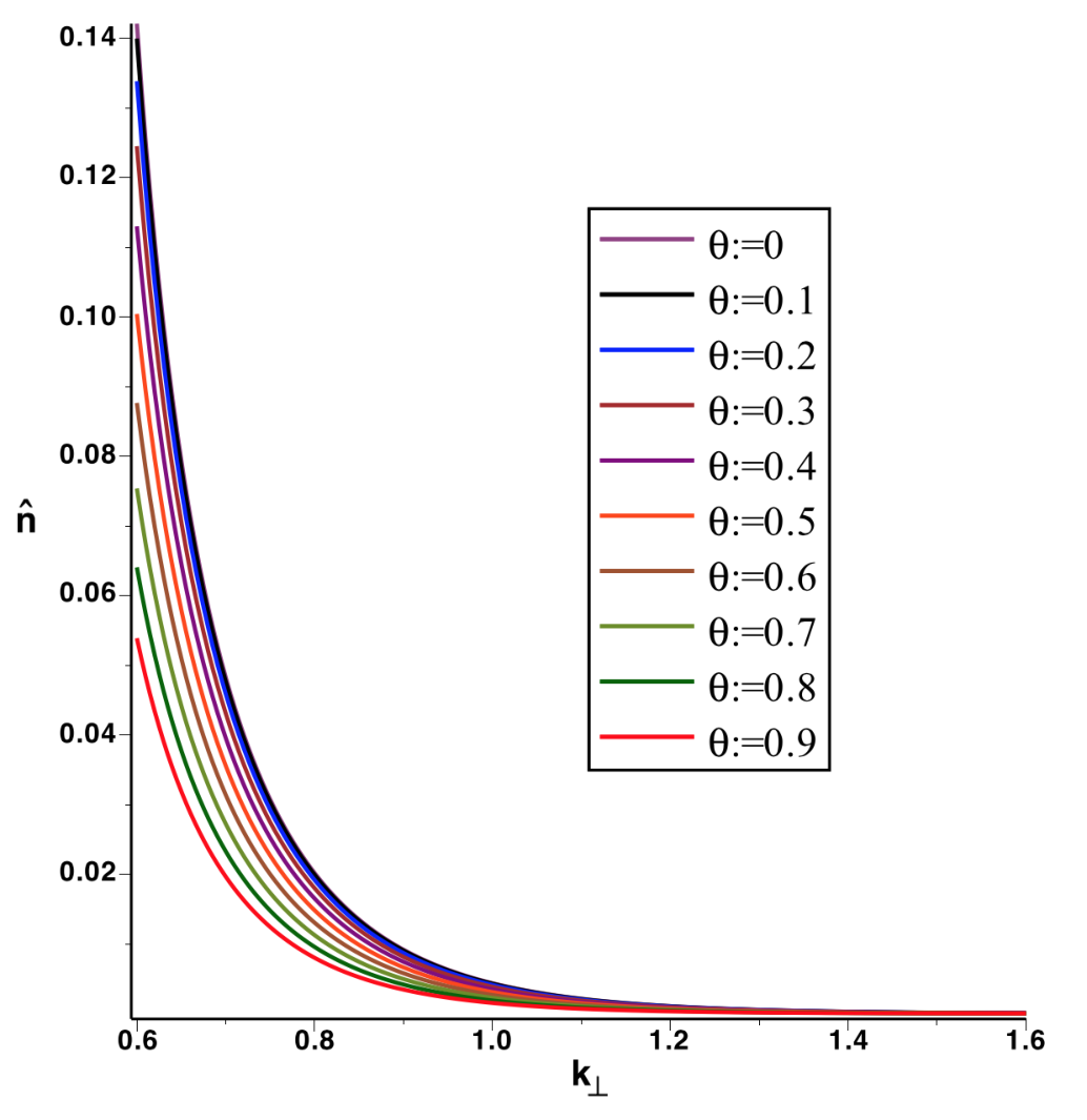
Figure 2: The number density n^\hat{n} as a function of the k⟂k_{\perp}-frequency modes and the noncommutativity θ\theta parameter

In Ref. [5] in region II, the N.C. θ\theta parameter was interpreted as playing the role of antigravity (e.g. quintessence, dark energy, etc.). However, in this paper (bosonic case) as θ\theta increases, SQ.ES_{Q.E} decreases. This does not mean that θ\theta plays the role of gravity. In fact, in the bosonic case, the B.E.C. phenomenon which of course depends on θ\theta increases more than the gravity generated by θ\theta, so that overall, the behavior of SQ.ES_{Q.E} looks like we have gravity.
Thus, at the end with B.E.C together with antigravitational effects of N.C parameter, SQ.ES_{Q.E} becomes a decreasing function of θ\theta. Therefore, we can say that θ\theta generates not only antigravity but the B.E.C phenomenon as well. To have a better understanding, let us consider the number density n^\hat{n} (see FIG. 2). Notice that n^\hat{n} and SQ.ES_{Q.E} have the same behavior with respect to k⟂k_{\perp} or θ\theta.

Refer to caption
Figure 3: The chemical potential μ\mu as a function of the k⟂k_{\perp}-frequency modes and the noncommutativity θ\theta parameter

Straightforward calculations show that the chemical potential μ\mu is proportional to log⁡(n^​e2​π​α1+n^)\log\left(\frac{\hat{n}e^{2\pi\alpha}}{1+\hat{n}}\right), where α=(1/8)​25​k⟂2​θ2+64​k⟂2−16\alpha=\left(1/8\right)\sqrt{25k_{\perp}^{2}\theta^{2}+64k_{\perp}^{2}-16} and it can be shown to be negative (see FIG. 3). The reason for μ\mu being negative is that in the thermodynamical equilibrium where μ\mu is proportional to −Δ​SQ.EΔ​n^-\frac{\Delta S_{Q.E}}{\Delta\hat{n}} and Δ​SQ.E\Delta S_{Q.E} is an increasing function of Δ​n^\Delta\hat{n}, the ratio Δ​SQ.EΔ​n^\frac{\Delta S_{Q.E}}{\Delta\hat{n}} is positive and therefore μ\mu is negative. Now, if μ{\mu} goes to 00 implies that α\alpha goes to 00, leading to k⟂=425​θ2+64k_{\perp}=\frac{4}{\sqrt{25\theta^{2}+64}}, which means that SQ.ES_{Q.E} goes to SQ.Em​a​xS_{Q.E}^{max} (maximally bipartite boson-antiboson entangled state), and the fugacity zz goes to 11. In other words, we have a critical point and one has a sort of B.E.C phenomenon.

Refer to caption
Figure 4: SQ.ES_{Q.E} as a function of the k⟂k_{\perp}-frequency modes for various values of the N.C.θ\theta parameter
Refer to caption
Figure 5: Density plot of SQ.ES_{Q.E} as a function of the k⟂k_{\perp}-frequency modes for various values of the N.C.θ\theta parameter
Refer to caption
Figure 6: Contours plot of n^\hat{n} as a function of the k⟂k_{\perp}-frequency modes for various values of the N.C.θ\theta parameter
Refer to caption
Figure 7: Contours plot of SQ.ES_{Q.E} as a function of the k⟂k_{\perp}-frequency modes for various values of the N.C.θ\theta parameter

Figure 5 displays SQ.ES_{Q.E} as a function of θ\theta and k⟂k_{\perp}. Figure 5 shows the density plot of SQ.ES_{Q.E} as a function of k⟂k_{\perp} for various values of θ\theta. Figures 7 and 7 illustrate contours plot of the number density n^\hat{n} and SQ.ES_{Q.E} as a function of k⟂k_{\perp} and θ\theta respectively. Figure 8 represents the chemical potential μ\mu as a function of SQ.Em​a​xS_{Q.E}^{max}.

Notice that as SQ.Em​a​xS_{Q.E}^{max} increases, μ\mu increases too. The reason is that, if μ\mu increases the boson-antiboson pair creation rate increases and therefore the B.E.C. phenomenon becomes more important leading to an increase in SQ.ES_{Q.E} (or SQ.Em​a​xS_{Q.E}^{max}), or a decrease of θ\theta (SQ.Em​a​xS_{Q.E}^{max} is a decreasing function of θ\theta).

Refer to caption
Figure 8: The chemical potential μ\mu as a function of SQ.Em​a​xS_{Q.E}^{max}

4 Conclusion

Throughout this paper, we have studied the creation of quantum entanglement between pairs of massless boson-antiboson particles within the framework of the N.C. Bianchi I universe as well as its relationship to thermodynamics. We have first derived the modified N.C. Klein Gordon equation for massless bosons and its solutions. Also, due to the complexity of the N.C. anisotropic Bianchi I spacetime structure, the behaviors of SQ.ES_{Q.E} as a function of k⟂−k_{\perp}- frequency modes are not trivial and different from those obtained in Ref. [16] for the case of isotropic F.R.W. universe (taking a particular solvable case). According to our obtained results, the structure and the deformation of the spacetime, as well as the involved particles (fermions or bosons), affect not only the behavior of SQ.ES_{Q.E} as a function of k⟂k_{\perp} but also the position of SQ.Em​a​xS_{Q.E}^{max} as well. It should be noted that, in Ref. [16], due to the spacetime isotropy, the authors have noticed that for massless bosons one has a maximum value of SQ.ES_{Q.E} independently of the value of kzk_{z} (not k⟂k_{\perp}). Our results show that even with massless particles, one can have a non vanishing quantum entanglement which depends only on k⟂=kx2+ky2k_{\perp}=\sqrt{k_{x}^{2}+k_{y}^{2}} (because of the Bianchi I spacetime anisotropy and the choice of the N.C. θ\theta parameter). Similar conclusions were obtained in our previous work (Ref. [5]) concerning the fermionic case and compared to Ref. [12]. Thus, the arguments in Refs.[12, 16] do not hold in general. We have also discussed the behavior of some thermodynamic quantities (like the chemical potential μ\mu) as a function of k⟂−k_{\perp}- frequency modes and the N.C. θ\theta parameter. We have also shown that the behavior of SQ.ES_{Q.E} depends on the kind of the involved particles (boson or fermions) during the pair creation process as well as on the structure and deformation of spacetime. Contrary to Ref. [16] and because of the spacetime deformation, the SQ.ES_{Q.E} for massless bosons does not always have a maximum but do depend on the k⟂k_{\perp}. Notice also that our results depend only on the transverse component k⟂k_{\perp} for some allowed values starting from k⟂m​i​n=425​θ2+64k_{\perp}^{min}=\frac{4}{\sqrt{25\theta^{2}+64}} (not the whole components of kk). The maximally entangled state where SQ.E→SQ.Em​a​xS_{Q.E}\rightarrow S_{Q.E}^{max} depends strongly on the N.C. θ\theta parameter and knowing the position of SQ.Em​a​xS_{Q.E}^{max} one can get information about certain thermodynamic quantities (like the chemical potential μ\mu) of the N.C. Bianchi I universe and vice versa. More interesting, we have shown, our numerical results confirm it, that for the minimal value of k⟂k_{\perp} we have a sort of phase transition (critical point) between the out of equilibrium and equilibrium regions (regions I and II). Furthermore, the N.C. θ\theta parameter plays the role of antigravity and contributes to increase the B.E.C. phenomenon. Finally and unlike our previous result in Ref. [5] (where |θ|≤85|\theta|\leq\frac{8}{5}), here we cannot get an upper bound of the N.C. θ\theta parameter. More studies are under investigation.

Acknowledgments

We are very grateful to the Algerian Ministry of Higher Education and Scientific Research and D.G.R.S.D.T. for financial support. This work is also supported by the P.R.F.U. project.

Appendix A N.C. Mathematical Formalism

The N.C. metric is given by (see Refs. [29], [37]) :

g^μ​ν=12​(e^μb∗e^ν​b+e^νb∗e^μ​b)\hat{g}_{\mu\nu}=\frac{1}{2}\left(\hat{e}^{b}_{\mu}\ast\hat{e}_{\nu b}+\hat{e}^{b}_{\nu}\ast\hat{e}_{\mu b}\right) (44)

where, the N.C. Vierbeins e^μa\hat{e}^{a}_{\mu} up to O⁡(θ2)O(\theta^{2}) are (see Ref. [5]):

e^μa=eμa−i​θν​ρ​eμ​ν​ρa+θν​ρ​θλ​τ​eμ​ν​ρ​λ​τa+O⁡(θ3)\hat{e}^{a}_{\mu}=e^{a}_{\mu}-i\,\theta^{\nu\rho}\,e^{a}_{\mu\nu\rho}+\theta^{\nu\rho}\,\theta^{\lambda\tau}\,e^{a}_{\mu\nu\rho\lambda\tau}+O\left(\theta^{3}\right) (45)

and

eμ​ν​ρa=14​[ωνa​c​∂ρeμd+(∂ρωμa​c+Rρ​μa​c)​eνd]​ηc​de^{a}_{\mu\nu\rho}=\frac{1}{4}\left[\omega^{ac}_{\nu}\,\partial_{\rho}\,e^{d}_{\mu}+\left(\partial_{\rho}\,\omega^{ac}_{\mu}+R^{ac}_{\rho\mu}\right)e^{d}_{\nu}\right]\eta_{cd} (46)
eμ​ν​ρ​λ​τa\displaystyle e^{a}_{\mu\nu\rho\lambda\tau} =\displaystyle= 132[2{Rτ​ν,Rμ​ρ}a​beλc−ωλa​b(DρRτ​μc​d+∂ρRτ​μc​d)eνmηd​m\displaystyle\frac{1}{32}[2\{R_{\tau\nu},R_{\mu\rho}\}^{ab}\,e^{c}_{\lambda}-\omega^{ab}_{\lambda}(D_{\rho}\,R^{cd}_{\tau\mu}+\partial_{\rho}\,R^{cd}_{\tau\mu})\,e^{m}_{\nu}\,\eta_{dm} (47)
−{ων,(Dρ​Rτ​μ+∂ρRτ​μ)}a​b​eλc−∂τ{ων,(∂ρωμ+Rρ​μ)}a​b​eλc\displaystyle-\{\omega_{\nu},(D_{\rho}\,R_{\tau\mu}+\partial_{\rho}\,R_{\tau\mu})\}^{ab}\,e^{c}_{\lambda}-\partial_{\tau}\{\omega_{\nu},(\partial_{\rho}\,\omega_{\mu}+R_{\rho\mu})\}^{ab}\,e^{c}_{\lambda}
−ωλa​b∂τ(ωνc​d∂ρeμm+(∂ρωμc​d+Rρ​μc​d)eνm)ηd​m+2∂νωλa​b∂ρ∂τeμc\displaystyle-\omega^{ab}_{\lambda}\,\partial_{\tau}(\omega^{cd}_{\nu}\,\partial_{\rho}\,e^{m}_{\mu}+(\partial_{\rho}\,\omega^{cd}_{\mu}+R^{cd}_{\rho\mu})\,e^{m}_{\nu})\,\eta_{dm}+2\partial_{\nu}\,\omega^{ab}_{\lambda}\,\partial_{\rho}\,\partial_{\tau}\,e^{c}_{\mu}
−2∂ρ(∂τωμa​b+Rτ​μa​b)∂νeλc−{ων,(∂ρωλ+Rρ​λ)}a​b∂τeμc\displaystyle-2\partial_{\rho}(\partial_{\tau}\,\omega^{ab}_{\mu}+R^{ab}_{\tau\mu})\,\partial_{\nu}\,e^{c}_{\lambda}-\{\omega_{\nu},(\partial_{\rho}\omega_{\lambda}+R_{\rho\lambda})\}^{ab}\,\partial_{\tau}\,e^{c}_{\mu}
−(∂τωμa​b+Rτ​μa​b)(ωνc​d∂ρeλm+(∂ρωλc​d+Rρ​λc​d)eνmηd​m)]ηb​c\displaystyle-(\partial_{\tau}\,\omega^{ab}_{\mu}+R^{ab}_{\tau\mu})(\omega^{cd}_{\nu}\,\partial_{\rho}\,e^{m}_{\lambda}+(\partial_{\rho}\,\omega^{cd}_{\lambda}+R^{cd}_{\rho\lambda})\,e^{m}_{\nu}\,\eta_{dm})]\,\eta_{bc}

here Rμ​νa​bR^{ab}_{\mu\nu} is the strength field associated with the commutative spin connections ωμa​b\omega^{ab}_{\mu} and is defined as:

Rμ​νa​b=∂μωνa​b−∂νωμa​b+(ωμa​c​ωνd​b−ωνa​c​ωμd​b)​ηc​dR^{ab}_{\mu\nu}=\partial_{\mu}\,\omega^{ab}_{\nu}-\partial_{\nu}\,\omega^{ab}_{\mu}+\left(\omega^{ac}_{\mu}\,\omega^{db}_{\nu}-\omega^{ac}_{\nu}\,\omega^{db}_{\mu}\right)\,\eta_{cd} (48)

(ηa​b\eta_{ab} is the Minkowski metric).
The N.C. spin connections ω^μA​B\hat{\omega}^{AB}_{\mu} up to O⁡(θ2)O(\theta^{2}) are:

ω^μA​B=ωμA​B−i​θν​ρ​ωμ​ν​ρA​B+θν​ρ​θλ​τ​ωμ​ν​ρ​λ​τA​B+….\hat{\omega}^{AB}_{\mu}=\omega^{AB}_{\mu}-i\,\theta^{\nu\rho}\,\omega^{AB}_{\mu\nu\rho}+\theta^{\nu\rho}\,\theta^{\lambda\tau}\,\omega^{AB}_{\mu\nu\rho\lambda\tau}+.... (49)

where

ωμ​ν​ρA​B=14​{ων,∂ρων+Rρ​μ}A​B\omega^{AB}_{\mu\nu\rho}=\frac{1}{4}\{\omega_{\nu},\partial_{\rho}\,\omega_{\nu}+R_{\rho\mu}\}^{AB} (50)
ωμ​ν​ρ​λ​τA​B\displaystyle\omega^{AB}_{\mu\nu\rho\lambda\tau} =\displaystyle= 132​(−{ωλ,∂τ{ων,∂ρωμ+Rρ​μ}}+2​{ωλ,{Rτ​ν,Rμ​ρ}}CLOSE\displaystyle\frac{1}{32}(-\{\omega_{\lambda},\partial_{\tau}\{\omega_{\nu},\partial_{\rho}\,\omega_{\mu}+R_{\rho\mu}\}\}+2\{\omega_{\lambda},\{R_{\tau\nu},R_{\mu\rho}\}\} (51)
−{ωλ,{ων,Dρ​Rτ​μ+∂ρRτ​μ}}−{{ων,∂ρωλ+Rρ​λ},(∂τωμ+Rτ​μ)}\displaystyle-\{\omega_{\lambda},\{\omega_{\nu},D_{\rho}\,R_{\tau\mu}+\partial_{\rho}\,R_{\tau\mu}\}\}-\{\{\omega_{\nu},\partial_{\rho}\,\omega_{\lambda}+R_{\rho\lambda}\},(\partial_{\tau}\,\omega_{\mu}+R_{\tau\mu})\}
OPEN+2​[∂νωλ,∂ρ(∂τωμ+Rτ​μ)])A​B\displaystyle+2[\partial_{\nu}\,\omega_{\lambda},\partial_{\rho}(\partial_{\tau}\,\omega_{\mu}+R_{\tau\mu})])^{AB}

here

{α,β}A​B=αA​C​βCB+βA​C​αCB\{\alpha,\beta\}^{AB}=\alpha^{AC}\,\beta^{B}_{C}+\beta^{AC}\,\alpha^{B}_{C} (52)
[α,β]A​B=αA​C​βCB−βA​C​αCB[\alpha,\beta]^{AB}=\alpha^{AC}\,\beta^{B}_{C}-\beta^{AC}\,\alpha^{B}_{C} (53)

and

Dμ​Rρ​σA​B=∂μRρ​σA​B+(ωμA​C+Rρ​σD​B+ωμB​C​Rρ​σD​A)​ηC​DD_{\mu}\,R^{AB}_{\rho\sigma}=\partial_{\mu}\,R^{AB}_{\rho\sigma}+(\omega^{AC}_{\mu}+R^{DB}_{\rho\sigma}+\omega^{BC}_{\mu}\,R^{DA}_{\rho\sigma})\,\eta_{CD} (54)

We propose the following action:

S=12​k2​∫d4​x​(ℒG+ℒS​C)S=\frac{1}{2{k}^{2}}\int d^{4}x\left(\mathcal{L}_{G}+\mathcal{L}_{SC}\right) (55)

where ℒG\mathcal{L}_{G} and ℒS​C\mathcal{L}_{SC} stand for the pure gravity and matter scalar densities corresponding to the charged scalar particle.
We define

ℒG=e^∗R^\mathcal{L}_{G}=\hat{e}\ast\hat{R} (56)

and

ℒS​C=e^∗(g^μ​ν∗(D^μ​φ^)†∗D^ν​φ^)\mathcal{L}_{SC}=\hat{e}\ast\left(\hat{g}^{\mu\nu}\ast\left(\hat{D}_{\mu}\hat{\varphi}\right)^{\dagger}\ast\hat{D}_{\nu}\hat{\varphi}\right) (57)

with :

R^=e^∗aμ∗e^∗bν∗R^μ​νa​b\hat{R}=\hat{e}^{\mu}_{\ast a}\ast\hat{e}^{\nu}_{\ast b}\ast\hat{R}^{ab}_{\mu\nu} (58)

Applying the principle of least action, it is easy to show that the modified field equations are given by:

∂ℒ∂φ^−∂μ∂ℒ∂(∂μφ^)+∂μ∂ν∂ℒ∂(∂μ∂νφ^)−∂μ∂ν∂σ∂ℒ∂(∂μ∂ν∂σφ^)+O⁡(θ3)=0\frac{\partial\mathcal{L}}{\partial\hat{\varphi}}-\partial_{\mu}\frac{\partial\mathcal{L}}{\partial\left(\partial_{\mu}\hat{\varphi}\right)}+\partial_{\mu}\partial_{\nu}\frac{\partial\mathcal{L}}{\partial\left(\partial_{\mu}\partial_{\nu}\hat{\varphi}\right)}-\partial_{\mu}\partial_{\nu}\partial_{\sigma}\frac{\partial\mathcal{L}}{\partial\left(\partial_{\mu}\partial_{\nu}\partial_{\sigma}\hat{\varphi}\right)}+O\left(\theta^{3}\right)=0 (59)

References

  • [1] S. Hill and W. K. Wootters, Phys. Rev. Lett 78, 5022 (1997).
  • [2] V. Vedral, M. B. Plenio, M. A. Rippin and P. L. Knight, Phys. Rev. Lett 78, 2275 (1997).
  • [3] D. C. Santos, Entanglement: from its mathematical description to its experimental observation, PhD Thesis, University of Barcelona (2008).
  • [4] M. F. Ghiti, N. Mebarki and M. T. Rouabah, Paraquantum Entangled Coherent and Squeezed States: New Type of Entanglement, in Proc. 8th Int. Conf. On Progress in Theoretical Physics, eds. N. Mebarki, J. Mimouni, N. Belaloui and K. Ait Moussa, (Meleville, New York, 2012), p. 238.
  • [5] M. F. Ghiti, N. Mebarki and H. Aissaoui, Int. J. Modern. Phys. A 30, 1550141 (2015).
  • [6] M. F. Ghiti and H. Aissaoui, Sciences and Technology A 40, 65-69 (2014).
  • [7] N. Mebarki, A. Morchedi and H. Aissaoui, Int. Jour. Theor. Phys. 54, 4124 (2015).
  • [8] H. Garcia-Compéan and F. Robledo-Padilla, Class. Quantum Grav 30, 235012 (2013).
  • [9] I. Fuentes, R. B. Mann, E. M. Martinez and S. Moradi, Phys. Rev. D 82, 045030 (2010).
  • [10] J. Hu and H. Yu, Phys. Rev. D 88, 104003 (2013).
  • [11] L. N. Machado, H. A. S. Costa, I. G. da Paz, M. Sampaio and J. B. Araujo, Phys. Rev. D 98, 125009 (2018).
  • [12] I. Fuentes, R. B. Mann, E. M. Martinez and S. Moradi, Phys. Rev. D 82, 045030 (2010).
  • [13] J. L. Ball, I. Fuentes-Schuller and F. P. Schuller, Phys. Lett. A 359, 550 (2006).
  • [14] D. E. Bruschi, A. Dragan, I. Fuentes and J. Louko, Phys. Rev. D 86, 025026 (2012).
  • [15] Y. Li, Q. Mao and Y. Shi, Phys. Rev. A 99, 032340 (2019)
  • [16] Z. Ebadi and B. Mirza, Annals of Physics 351, 363 (2014).
  • [17] Peter. K.F. Kuhfitting, J. Mod. Phys 8, 323 (2017).
  • [18] S. Kawamoto et al, Class. Quant. Grav 34, 177001 (2017).
  • [19] M. M. Ettefaghi. Phys. Rev. D 79, 065022 (2009).
  • [20] N. Mebarki, Dark Energy, Induced Cosmological Constant and Matter - Antimatter Asymmetry From Non Commutative Geometry, in Proc. 3rd Int Meeting. On the Frontiers of Physics , eds. S. P. Chia, K. Ratnavelu and M. R. Muhamad, (Melville, New York, 2009), p 38.
  • [21] Z. Rezaei and S. Peyman Zakeri, e-Print 2007.01501[hep-ph] (2020).
  • [22] A. Espinoza-Garcia and J. Socorro, 10th Workshop of the gravitation and Mathematical physics Division of the Mexican Physical Society, eds. R. B. Bárcenas et al, 545 2014.
  • [23] W. Behr, N. G. Deshpande, G. Duplancic, P. Schupp, J. Trampetic and J. Wess, Eur. Phys. J. C 29, 441 (2003).
  • [24] M. Buric, D. Latas, V. Radovanovic and J. Trampetic, Phys. Rev. D 75, 097701 (2007).
  • [25] M. Haghighat, M. Ettefaghi and M. Zeinali, Phys. Rev. D 73, 013007 (2006).
  • [26] P. K. Das, N. G. Deshpande and G. Rajasekaran, Phys. Rev. D 77, 035010 (2008).
  • [27] A. Prakash, A. Mitra and P. K. Das, Phys. Rev. D 82, 055020 (2010).
  • [28] R. Horvat and J. Trampetic, Phys. Lett. B 710, 219 (2012).
  • [29] N. Mebarki, L. Khodja and S. Zaim, Electron. J. Theor. Phys. 7, 181 (2010).
  • [30] N. Mebarki, S. Zaim, L. Khodja and H. Aissaoui, Phys. Scri. 78, 045101 (2008).
  • [31] S. Zaim and L. Khodja, Phys. Scr. 81, 055103 (2010).
  • [32] N. Seiberg and E. Witten, J. High Energy Phys. 09, 032 (1999).
  • [33] L. Parker, Phys. Rev. Lett. 21, 562 (1968).
  • [34] V. M. Villalba and W. Greiner, Phys. Rev. D. 65, 025007 (2001).
  • [35] V. M. Villalba and W. Greiner, Mod. Phys. Lett. A 17, 1883 (2002).
  • [36] M. Abramowitz and I. Stegun, Handbook of Mathematical Functions with Formulas, Graphs, and Mathematical Tables (Dover Publications, New York, 1964).
  • [37] M. Chaichian, A. Tureanu and G. Zet, Phys. Lett. B 660, 573 (2008).