Fast Incremental Expectation Maximization for finite-sum optimization: nonasymptotic convergence. Thanks: This work is partially supported by the Fondation Simone et Cino Del Duca through the project OpSiMorE; by the French Agence Nationale de la Recherche (ANR), project under reference ANR-PRC-CE23 MASDOL and Chair ANR of research and teaching in artificial intelligence - SCAI Statistics and Computation for AI; and by the Russian Academic Excellence Project ’5-100’.

G. Fort Affiliation: Institut de Mathématiques de Toulouse & CNRS, France; gersende.fort@math.univ-toulouse.fr P. Gach Affiliation: Institut de Mathématiques de Toulouse & Université Toulouse 3, France; pierre.gach@math.univ-toulouse.fr E. Moulines Affiliation: CMAP & Ecole Polytechnique, France; eric.moulines@polytechnique.edu

Abstract

Fast Incremental Expectation Maximization (FIEM) is a version of the EM framework for large datasets. In this paper, we first recast FIEM and other incremental EM type algorithms in the Stochastic Approximation within EM framework. Then, we provide nonasymptotic bounds for the convergence in expectation as a function of the number of examples $n$ and of the maximal number of iterations $K_{\mathrm{max}}$ . We propose two strategies for achieving an $\epsilon$ -approximate stationary point, respectively with $K_{\mathrm{max}}=O(n^{2/3}/\epsilon)$ and $K_{\mathrm{max}}=O(\sqrt{n}/\epsilon^{3/2})$ , both strategies relying on a random termination rule before $K_{\mathrm{max}}$ and on a constant step size in the Stochastic Approximation step. Our bounds provide some improvements on the literature. First, they allow $K_{\mathrm{max}}$ to scale as $\sqrt{n}$ which is better than $n^{2/3}$ which was the best rate obtained so far; it is at the cost of a larger dependence upon the tolerance $\epsilon$ , thus making this control relevant for small to medium accuracy with respect to the number of examples $n$ . Second, for the $n^{2/3}$ -rate, the numerical illustrations show that thanks to an optimized choice of the step size and of the bounds in terms of quantities characterizing the optimization problem at hand, our results design a less conservative choice of the step size and provide a better control of the convergence in expectation.

keywords: Computational Statistical Learning Large Scale Learning Incremental Expectation Maximization algorithm Momentum Stochastic Approximation Finite-sum optimization.

Mathematics Subject Classification (2010) MSC: 65C60 68Q32 65K10

1 Introduction

The Expectation Maximization (EM) algorithm was introduced by Dempster et al. 1977 to solve a non-convex optimization problem on $\Theta\subseteq\mathbb{R}^{d}$ when the objective function $F$ is defined through an integral:

(1)

F(\theta)\stackrel{{\scriptstyle\mathrm{def}}}{{=}}-\frac{1}{n}\log\int_{\mathsf{Z}_{n}}G(z;\theta)\ \mu_{n}(\mathrm{d}z)\;,

for $n\in{\mathbb{N}}\setminus\{0\}$ , a positive function $G$ and a $\sigma$ -finite positive measure $\mu_{n}$ on a measurable space $(\mathsf{Z}_{n},\mathcal{Z}_{n})$ . EM is a Majorize-Minimization (MM) algorithm which, based on the current value of the iterate $\theta_{\mathrm{curr}}$ , defines a majorizing function $\theta\mapsto\mathsf{Q}(\theta,\theta_{\mathrm{curr}})$ given, up to an additive constant, by

\mathsf{Q}(\theta,\theta_{\mathrm{curr}})\stackrel{{\scriptstyle\mathrm{def}}}{{=}}-\frac{1}{n}\int_{\mathsf{Z}_{n}}\log G(z;\theta)\ G(z;\theta_{\mathrm{curr}})\exp(n\,F(\theta_{\mathrm{curr}}))\mu_{n}(\mathrm{d}z)\;.

The next iterate is chosen to be the/a minimum of $\mathsf{Q}(\cdot,\theta_{\mathrm{curr}})$ . Each iteration of EM is divided into two steps. In the E step (expectation step), a surrogate function is computed. In the M step (minimization step), the surrogate function is minimized. The computation of the $\mathsf{Q}$ function is straightforward when there exist functions $\Phi:\Theta\to\mathbb{R}^{q}$ and $S:\mathsf{Z}_{n}\to\mathbb{R}^{q}$ such that $n^{-1}\log G(z;\theta)=\left\langle S(z),\Phi(\theta)\right\rangle$ ; this yields $\mathsf{Q}(\theta,\theta_{\mathrm{curr}})=-\left\langle\bar{s}(\theta_{\mathrm{curr}}),\Phi(\theta)\right\rangle$ where $\bar{s}(\theta_{\mathrm{curr}})$ denotes the expectation of the function $S$ with respect to (w.r.t.) the probability measure

\pi_{\theta_{\mathrm{curr}}}(\mathrm{d}z)\stackrel{{\scriptstyle\mathrm{def}}}{{=}}G(z;\theta_{\mathrm{curr}})\exp(n\,F(\theta_{\mathrm{curr}}))\mu_{n}(\mathrm{d}z)\;.

This paper is concerned with the case $\mathsf{Z}_{n}$ is the $n$ -fold Cartesian product of the set $\mathsf{Z}$ (denoted by $\mathsf{Z}^{n}$ ), $z=(z_{1},\cdots,z_{n})\in\mathsf{Z}^{n}$ , $S(z)=n^{-1}\sum_{i=1}^{n}s_{i}(z_{i})$ , $\mu_{n}$ is the tensor product of the $\sigma$ -finite positive measure $\mu$ on the measurable space $(\mathsf{Z},\mathcal{Z})$ . This implies that

	$\displaystyle F(\theta)$	$\displaystyle=\frac{1}{n}\sum_{i=1}^{n}f_{i}(\theta)\;,$
	$\displaystyle f_{i}(\theta)$	$\displaystyle\stackrel{{\scriptstyle\mathrm{def}}}{{=}}-\log\int_{\mathsf{Z}}\exp(\left\langle s_{i}(z),\Phi(\theta)\right\rangle)\ \mu(\mathrm{d}z)\;;$
	$\displaystyle\bar{s}(\theta_{\mathrm{curr}})$	$\displaystyle\propto\frac{1}{n}\sum_{i=1}^{n}\int_{\mathsf{Z}}s_{i}(z)\frac{\exp(\left\langle s_{i}(z),\Phi(\theta_{\mathrm{curr}})\right\rangle)\,\mu(\mathrm{d}z)}{\int_{\mathsf{Z}}\exp(\left\langle s_{i}(z^{\prime}),\Phi(\theta_{\mathrm{curr}})\right\rangle)\mu(\mathrm{d}z^{\prime})}\;.$

This finite-sum framework is motivated by large scale learning problems. In such case, $n$ is the number of observations, assumed to be independent; the function $f_{i}$ stands for a possibly non-convex loss associated to the observation $\#i$ and can also include a penalty (or a regularization) term. In the statistical context, $F$ is the negative normalized log-likelihood of the $n$ observations in a latent variable model, and $G$ is the complete likelihood; when $\log G(z;\theta)\propto\left\langle S(z),\Phi(\theta)\right\rangle$ , it belongs to the curved exponential family (see e.g. Brown 1986 and Sundberg 2019).

When $n$ is large, the computation of $\bar{s}(\theta_{\mathrm{curr}})$ is computationally costly and should be avoided. We consider incremental algorithms which use, at each iteration, a mini-batch of examples. The computational complexity of these procedures typically displays a trade-off between the loss of information incurred by the use of a subset of the observations, and a faster progress toward the solutions since the parameters can be updated more often.

A pioneering work in this direction is the incremental EM by Neal and Hinton 1998: the data set is divided into $B$ blocks and a single block is visited between each parameter update. The $\mathsf{Q}$ function of incremental EM is again a sum over $n$ terms, but each E step consists in updating only a block of terms in this sum (see Ng and McLachlan 2003).

The Online EM algorithm by Cappé and Moulines 2009 was originally designed to process data streams. It replaces the computation of $\bar{s}(\theta_{\mathrm{curr}})$ by an iteration of a Stochastic Approximation (SA) algorithm (see Robbins and Monro 1951). Online EM in the finite sum setting is closely related to Stochastic Gradient Descent. Improved versions were considered by Chen et al. 2018 and by Karimi et al. 2019b which introduced respectively Stochastic EM with Variance Reduction (sEM-vr) and Fast Incremental EM (FIEM) as variance reduction techniques within Online EM as an echo to Stochastic Variance Reduced Gradient (SVRG, Johnson and Zhang 2013) and Stochastic Averaged Gradient (SAGA, Defazio et al. 2014) introduced as variance reduction techniques within Stochastic Gradient Descent.

In this paper, we aim to study such incremental EM methods combined with a SA approach. The first goal of this paper is to cast Online EM, incremental EM and FIEM into a framework called hereafter Stochastic Approximation within EM approaches; see subsection 2.2. We show that the E step of FIEM can be seen as the combination of an SA update and of a control variate; we propose to optimize the trade-off between update and variance reduction, which yields to the opt-FIEM algorithm (see also section 4 for a numerical exploration).

The second and main objective of this paper, is to derive nonasymptotic upper bounds for the convergence in expectation of FIEM (see section 3).

Following Ghadimi and Lan 2013 (see also Allen-Zhu and Hazan 2016, Reddi et al. 2016, Fang et al. 2018, Zhou et al. 2018 and Karimi et al. 2019b), we propose to fix a maximal length $K_{\mathrm{max}}$ and terminate a path $\{\theta^{k},k\geq 0\}$ of the algorithm at some random time $K$ uniformly sampled from $\{0,\ldots,K_{\mathrm{max}}-1\}$ prior the run and independently of it; our bounds control the expectation $\mathbb{E}\left[\|\nabla F(\theta^{K})\|^{2}\right]$ and as a corollary, we discuss how to fix $K_{\mathrm{max}}$ as a function of the sample size $n$ in order to reach an $\epsilon$ -approximate stationary point i.e. to find $\hat{\theta}^{K,\epsilon}$ such that $\mathbb{E}\left[\|\nabla F(\hat{\theta}^{K,\epsilon})\|^{2}\right]\leq\epsilon$ . Such a property is sometimes called $\epsilon$ -accuracy in expectation (see e.g. (Reddi et al. 2016, Definition 1)).

Karimi et al. 2019b established that incremental EM, which picks at random one example per iteration, reaches $\epsilon$ -accuracy by choosing $K_{\mathrm{max}}=O(n\epsilon^{-1})$ : even if the algorithm is terminated at a random time $K$ , this random time is chosen as a function of $K_{\mathrm{max}}$ which has to increase linearly with the size $n$ of the data set. They also prove that for FIEM, $\epsilon$ -approximate stationarity is reached with $K_{\mathrm{max}}=O(n^{2/3}\epsilon^{-1})$ - here again, with one example picked at random per iteration. For these reasons, FIEM is preferable especially when $n$ is large (see section 5 for a numerical illustration). Our major contribution in this paper is to show that for FIEM, the rate depends on the choice of some design parameters. By choosing a constant step size sequence in the SA step, depending upon $n$ as $O(n^{-2/3})$ , then $\epsilon$ -accuracy requires $K_{\mathrm{max}}=O(n^{2/3}\epsilon^{-1})$ ; we provide a choice of the step size (with an explicit dependence on the constants of the problem) and an explicit expression of the upper bound, which improve the results reported in Karimi et al. 2019b (see subsection 3.2; see also section 4 for illustration). We then prove in subsection 3.3 that $\epsilon$ -accuracy can be achieved with $K_{\mathrm{max}}=O(\sqrt{n}\epsilon^{-3/2})$ iterations using another strategy for the definition of the step size. Finally, we go beyond the uniform distribution for the random termination time $K$ by considering a large class of distributions on the set $\{0,\ldots,K_{\mathrm{max}}-1\}$ (see subsection 3.4).

Notations.

$\left\langle a,b\right\rangle$ denotes the standard Euclidean scalar product on $\mathbb{R}^{\ell}$ , for $\ell\geq 1$ ; and $\|a\|$ the associated norm. For a matrix $A$ , $A^{T}$ is its transpose. By convention, vectors are column vectors.
For a smooth function $\phi$ , $\dot{\phi}$ denotes its gradient; for a smooth real-valued function of several variables $\mathsf{L}$ , $\partial_{\tau}^{k}\mathsf{L}$ stands for the partial derivative of order $k$ with respect to the variable $\tau$ .
For a non negative integer $n$ , $[n]\stackrel{{\scriptstyle\mathrm{def}}}{{=}}\{0,\cdots,n\}$ and $[n]^{\star}\stackrel{{\scriptstyle\mathrm{def}}}{{=}}\{1,\cdots,n\}$ . $a\wedge b$ is the minimum of two real numbers $a,b$ . The big $O$ notation is used to leave out constants.
For a random variable $U$ , $\sigma(U)$ denotes the sigma algebra generated by $U$ .

2 Incremental EM algorithms for finite-sum optimization

2.1 EM in the expectation space

This paper deals with EM-based algorithms to solve

(2)

\operatorname{Argmin}_{\theta\in\Theta}F(\theta),\qquad F(\theta)\stackrel{{\scriptstyle\mathrm{def}}}{{=}}\frac{1}{n}\sum_{i=1}^{n}\mathcal{L}_{i}(\theta)+\mathsf{R}(\theta)\;,

where

(3)

\mathcal{L}_{i}(\theta)\stackrel{{\scriptstyle\mathrm{def}}}{{=}}-\log\int_{\mathsf{Z}}\tilde{h}_{i}(z)\ \exp\left(\left\langle s_{i}(z),\phi(\theta)\right\rangle\right)\ \mu(\mathrm{d}z)\;,

under the following assumption:

A 1.

$\Theta\subseteq\mathbb{R}^{d}$ is a measurable convex subset. $(\mathsf{Z},\mathcal{Z})$ is a measurable space and $\mu$ is a $\sigma$ -finite positive measure on $(\mathsf{Z},\mathcal{Z})$ . The functions $\mathsf{R}:\Theta\to\mathbb{R}$ , $\phi:\Theta\to\mathbb{R}^{q}$ and $\tilde{h}_{i}:\mathsf{Z}\to\mathbb{R}_{+}$ , $s_{i}:\mathsf{Z}\to\mathbb{R}^{q}$ for $i\in[n]^{\star}$ are measurable functions. Finally, for any $\theta\in\Theta$ and $i\in[n]^{\star}$ , $-\infty<\mathcal{L}_{i}(\theta)<\infty$ .

Under A1, for any $\theta\in\Theta$ and $i\in[n]^{\star}$ , the quantity $p_{i}(z;\theta)\,\mu(\mathrm{d}z)$ where

p_{i}(z;\theta)\stackrel{{\scriptstyle\mathrm{def}}}{{=}}\tilde{h}_{i}(z)\ \exp\left(\left\langle s_{i}(z),\phi(\theta)\right\rangle+\mathcal{L}_{i}(\theta)\right)\;,

defines a probability measure on $(\mathsf{Z},\mathcal{Z})$ . We assume that

A 2.

For all $\theta\in\Theta$ and $i\in[n]^{\star}$ , the expectation

\bar{s}_{i}(\theta)\stackrel{{\scriptstyle\mathrm{def}}}{{=}}\int_{\mathsf{Z}}s_{i}(z)\ p_{i}(z;\theta)\mu(\mathrm{d}z)

exists and is computationally tractable.

For any $\theta\in\Theta$ , define

(4)

\bar{s}(\theta)\stackrel{{\scriptstyle\mathrm{def}}}{{=}}\frac{1}{n}\sum_{i=1}^{n}\bar{s}_{i}(\theta)\;.

The framework defined by (2) and (3) covers many computational learning problems such as empirical risk minimization with non-convex losses: $\mathsf{R}$ may include a regularization condition on the parameter $\theta$ , $\mathcal{L}_{i}$ is the loss function associated to example $\#i$ and $n^{-1}\sum_{i=1}^{n}\mathcal{L}_{i}$ is the empirical loss. This framework includes negative log-likelihood inference in latent variable model (see e.g. Little and Rubin 2002), when the complete data likelihood is from a curved exponential family; in this framework, $z\mapsto p_{i}(z;\theta)\mu(\mathrm{d}z)$ is the a posteriori distribution of the latent variable $\#i$ .

Given $\theta^{\prime}\in\Theta$ , define the function $\overline{F}(\cdot,\theta^{\prime}):\Theta\to\mathbb{R}$ by

	$\displaystyle\overline{F}(\theta,\theta^{\prime})$	$\displaystyle\stackrel{{\scriptstyle\mathrm{def}}}{{=}}-\left\langle\bar{s}(\theta^{\prime}),\phi(\theta)\right\rangle+\mathsf{R}(\theta)+\frac{1}{n}\sum_{i=1}^{n}\mathcal{C}_{i}(\theta^{\prime})\;,$
	$\displaystyle\mathcal{C}_{i}(\theta^{\prime})$	$\displaystyle\stackrel{{\scriptstyle\mathrm{def}}}{{=}}\mathcal{L}_{i}(\theta^{\prime})+\left\langle\bar{s}_{i}(\theta^{\prime}),\phi(\theta^{\prime})\right\rangle\;.$

It is well known (see McLachlan and Krishnan 2008; Lange 2016; see also section 7 in the supplementary material) that $\{\overline{F}(\cdot,\theta^{\prime}),\theta^{\prime}\in\Theta\}$ is a family of majorizing function of the objective function $F$ from which a Majorize-Minimization approach for solving (2) can be derived. Define

(5)

\mathsf{L}(s,\cdot):\theta\mapsto-\left\langle s,\phi(\theta)\right\rangle+\mathsf{R}(\theta)

and consider the following assumption:

A 3.

For any $s\in{\mathbb{R}^{q}}$ , $\theta\mapsto\mathsf{L}(s,\theta)$ has a unique global minimum on $\Theta$ denoted $\mathsf{T}(s)$ .

In most successful applications of the EM algorithm, the function $\theta\mapsto\mathsf{L}(s,\theta)$ is strongly convex. Strong convexity is however not required here. Starting from the current point $\theta^{k}$ , the EM iterative scheme $\theta^{k+1}=\mathsf{T}\circ\bar{s}(\theta^{k})$ first computes a point in $\bar{s}(\Theta)$ through the expectation $\bar{s}$ , and then apply the map $\mathsf{T}$ to obtain the new iterate $\theta^{k+1}$ . It can therefore be described in the $\bar{s}(\Theta)$ -space, a space sometimes called the expectation space: define the sequence $\{\bar{s}^{k},\;k\in{\mathbb{N}}\}$ by $\bar{s}^{0}\in{\mathbb{R}^{q}}$ and for any $k\geq 0$

(6)

\displaystyle\bar{s}^{k+1}

\displaystyle\stackrel{{\scriptstyle\mathrm{def}}}{{=}}\bar{s}\circ\mathsf{T}(\bar{s}^{k})\;.

Sufficient conditions for the characterization of the limit points of any instance $\{\bar{s}^{k},k\geq 0\}$ as the critical points of $F\circ\mathsf{T}$ , for the convergence of the functional along the sequence $\{F\circ\mathsf{T}(\bar{s}^{k}),k\geq 0\}$ , or for the convergence of the iterates $\{\bar{s}^{k},k\geq 0\}$ exist in the literature (see e.g. Wu 1983; Lange 1995; Delyon et al. 1999 in the EM context and Zangwill 1967; Csiszár and Tusnády 1984; Gunawardana and Byrne 2005; Parizi et al. 2019 for general iterative MM algorithms). Proposition 2.1 characterizes the fixed points of $\mathsf{T}\circ\bar{s}$ and of $\bar{s}\circ\mathsf{T}$ under a set of conditions which will be adopted for the convergence analysis in Section 3.

A 4.

(i)

The functions $\phi$ and $\mathsf{R}$ are continuously differentiable on $\Theta^{v}$ where $\Theta^{v}\stackrel{{\scriptstyle\mathrm{def}}}{{=}}\Theta$ if $\Theta$ is open, or $\Theta^{v}$ is a neighborhood of $\Theta$ otherwise. $\mathsf{T}$ is continuously differentiable on ${\mathbb{R}^{q}}$ .
(ii)

The function $F$ is continuously differentiable on $\Theta^{v}$ and for any $\theta\in\Theta$ , we have

$\dot{F}(\theta)=-\left(\dot{\phi}(\theta)\right)^{T}\,\bar{s}(\theta)+\dot{\mathsf{R}}(\theta)\;.$
(iii)

For any $s\in{\mathbb{R}^{q}}$ , $B(s)\stackrel{{\scriptstyle\mathrm{def}}}{{=}}\dot{\left(\phi\circ\mathsf{T}\right)}(s)$ is a symmetric $q\times q$ matrix with positive minimal eigenvalue.

Under A1 to A4-(i) and the assumption that $\Theta$ and $\phi(\Theta)$ are open subsets of resp. $\mathbb{R}^{d}$ and $\mathbb{R}^{q}$ , then subsubsection 6.1.2 shows that A4-(ii) holds and the functions $\mathcal{L}_{i}$ are continuously differentiable on $\Theta$ for all $i\in[n]^{\star}$ .

Under A1, A3 and the assumptions that (i) $\mathsf{T}$ is continuously differentiable on ${\mathbb{R}^{q}}$ and (ii) for any $s\in{\mathbb{R}^{q}}$ , $\tau\mapsto\mathsf{L}(s,\tau)$ (see (5)) is twice continuously differentiable on $\Theta^{v}$ (defined in A4-(i)), then for any $s\in{\mathbb{R}^{q}}$ , $\partial^{2}_{\tau}\mathsf{L}(s,\mathsf{T}(s))$ is positive-definite and

B(s)=\left(\dot{\mathsf{T}}(s)\right)^{T}\ \partial_{\tau}^{2}\mathsf{L}(s,\mathsf{T}(s))\ \left(\dot{\mathsf{T}}(s)\right)\;;

see (Delyon et al. 1999, Lemma 2). Therefore, $B(s)$ is a symmetric matrix and if $\mathrm{rank}(\dot{\mathsf{T}}(s))=q=q\wedge d$ , its minimal eigenvalue is positive.

Proposition 1.

Assume A1, A2 and A3. Define the measurable functions $V:{\mathbb{R}^{q}}\to\mathbb{R}$ and $h:{\mathbb{R}^{q}}\to\mathbb{R}^{q}$ by

V(s)\stackrel{{\scriptstyle\mathrm{def}}}{{=}}F\circ\mathsf{T}(s)\;,\qquad h(s)\stackrel{{\scriptstyle\mathrm{def}}}{{=}}\bar{s}\circ\mathsf{T}(s)-s\;.

1.

If $s^{\star}$ is a fixed point of $\bar{s}\circ\mathsf{T}$ , then $\mathsf{T}(s^{\star})$ is a fixed point of $\mathsf{T}\circ\bar{s}$ . Conversely, if $\theta^{\star}$ is a fixed point of $\mathsf{T}\circ\bar{s}$ then $\bar{s}(\theta^{\star})$ is a fixed point of $\bar{s}\circ\mathsf{T}$ .
2.

Assume also A4. For all $s\in{\mathbb{R}^{q}}$ , we have $\dot{V}(s)=-B(s)\ h(s)$ , and the zeros of $h$ are the critical points of $V$ .

The proof is in subsubsection 6.1.1. As a conclusion, the EM algorithm summarized in Algorithm 10, is designed to converge to the zeros of

(7)

s\mapsto h(s)\stackrel{{\scriptstyle\mathrm{def}}}{{=}}\bar{s}\circ\mathsf{T}(s)-s\;,

which, for some models, are the critical points of $F\circ\mathsf{T}$ .

Data:

K_{\mathrm{max}}\in{\mathbb{N}}

\bar{s}^{0}\in{\mathbb{R}^{q}}

Result: The EM sequence:

\bar{s}^{k},k\in[K_{\mathrm{max}}]

for $k=0,\ldots,K_{\mathrm{max}}-1$ do 1

\bar{s}^{k+1}=\bar{s}\circ\mathsf{T}(\bar{s}^{k})

Algorithm 1 EM in the expectation space

2.2 Stochastic Approximation within EM

In the finite-sum framework, the number of expectation evaluations $\bar{s}_{i}$ per iteration of EM is the number $n$ of examples (see Line 1 of Algorithm 10 and (4)). It is therefore very costly in the large scale learning framework. We review in this section few alternatives of EM which all substitute the EM update $\bar{s}^{k+1}=\bar{s}\circ\mathsf{T}(\bar{s}^{k})$ (see Line 1 in Algorithm 10) with an update $\widehat{S}^{k}\to\widehat{S}^{k+1}$ of the form

(8)

\widehat{S}^{k+1}=\widehat{S}^{k}+\gamma_{k+1}s^{k+1}\;,

where $\{\gamma_{k},k\geq 1\}$ is a deterministic positive sequence of step sizes (also called learning rates) chosen by the user and $s^{k+1}$ is an approximation of $h(\widehat{S}^{k})=\bar{s}\circ\mathsf{T}(\widehat{S}^{k})-\widehat{S}^{k}$ . When it is a random approximation, the iterative algorithm described by (8) is a SA algorithm designed to target the zeros of the mean field $s\mapsto h(s)$ (see (7)); see e.g. Benveniste et al. 1990; Borkar 2008 for a general review on SA. Many stochastic approximations of EM can be described by (8): let us cite for example the Stochastic EM by Celeux and Diebolt 1985, the Monte Carlo EM (MCEM, introduced by Wei and Tanner 1990 and studied by Fort and Moulines 2003) which corresponds to $\gamma_{k+1}=1$ and the Stochastic Approximation EM (SAEM) introduced by Delyon et al. 1999.

In the finite-sum framework, observe from (7) that for any $s\in\mathbb{R}^{q}$ ,

(9)

h(s)=\mathbb{E}\left[\bar{s}_{I}\circ\mathsf{T}(s)+W\right]-s\;,

where $I$ is a uniform random variable on $[n]^{\star}$ and $W$ is a zero-mean random vector. Such an expression gives insights for the definition of SA schemes, including the combination with a variance reduction techniques through an adequate choice of $W$ (see e.g. (Glasserman 2004, Section 4.1.) for an introduction to control variates). We review below recent EM-based algorithms, designed for the finite-sum setting.

2.2.1 The Fast Incremental EM algorithm

Fast Incremental EM (FIEM) was introduced by Karimi et al. 2019b; it is given in Algorithm 2.

Data:

K_{\mathrm{max}}\in{\mathbb{N}}

\widehat{S}^{0}\in{\mathbb{R}^{q}}

\gamma_{k}\in\left(0,\infty\right)

for

k\in[K_{\mathrm{max}}]^{\star}

Result: The FIEM sequence:

\widehat{S}^{k},k\in[K_{\mathrm{max}}]

\mathsf{S}_{0,i}=\bar{s}_{i}\circ\mathsf{T}(\widehat{S}^{0})

for all

i\in[n]^{\star}

; 1

\widetilde{S}^{0}=n^{-1}\sum_{i=1}^{n}\mathsf{S}_{0,i}

; 2

for $k=0,\ldots,K_{\mathrm{max}}-1$ do 3

Sample

I_{k+1}

uniformly from

[n]^{\star}

; 4

\mathsf{S}_{k+1,i}=\mathsf{S}_{k,i}

for

i\neq I_{k+1}

; 5

\mathsf{S}_{k+1,I_{k+1}}=\bar{s}_{I_{k+1}}\circ\mathsf{T}(\widehat{S}^{k})

; 6

\widetilde{S}^{k+1}=\widetilde{S}^{k}+n^{-1}\left(\mathsf{S}_{k+1,I_{k+1}}-\mathsf{S}_{k,I_{k+1}}\right)

; 7

Sample

J_{k+1}

uniformly from

[n]^{\star}

; 8

\widehat{S}^{k+1}=\widehat{S}^{k}+\gamma_{k+1}(\bar{s}_{J_{k+1}}\circ\mathsf{T}(\widehat{S}^{k})-\widehat{S}^{k}+\widetilde{S}^{k+1}-\mathsf{S}_{k+1,J_{k+1}})

Algorithm 2 Fast Incremental EM

Lines 2 to 2 are a recursive computation of $n^{-1}\sum_{i=1}^{n}\mathsf{S}_{k+1,i}$ , stored in $\widetilde{S}^{k+1}$ , where for $k\geq 0$ ,

(10)

\mathsf{S}_{k+1,i}\stackrel{{\scriptstyle\mathrm{def}}}{{=}}\left\{\begin{array}[]{ll}\bar{s}_{I_{k+1}}\circ\mathsf{T}(\widehat{S}^{k})&\ \text{if $i=I_{k+1}$ \;,}\\ \mathsf{S}_{k,i}&\ \text{otherwise \;.}\end{array}\right.

This procedure avoids the computation of a sum with $n$ terms at each iteration of FIEM, but at the price of a memory footprint since the $\mathbb{R}^{q}$ -valued vectors $\mathsf{S}_{k,i}$ for $i\in[n\wedge K_{\mathrm{max}}]^{\star}$ have to be stored. Line 2 is of the form (8) with $s^{k+1}$ equal to the sum of two terms: $\bar{s}_{J_{k+1}}\circ\mathsf{T}(\widehat{S}^{k})-\widehat{S}^{k}$ is an oracle for $\mathbb{E}\left[\bar{s}_{I}\circ\mathsf{T}(s)-s\right]$ evaluated at $s=\widehat{S}^{k}$ ; and $W\stackrel{{\scriptstyle\mathrm{def}}}{{=}}\widetilde{S}^{k+1}-\mathsf{S}_{k+1,J_{k+1}}$ acts as a control variate, which conditionally to the past $\mathcal{F}_{k+1/2}\stackrel{{\scriptstyle\mathrm{def}}}{{=}}\sigma(\widehat{S}^{0},I_{1},J_{1},\ldots,I_{k},J_{k},I_{k+1}\}$ , is centered. A natural extension, which is not addressed in this paper, is to replace the draws $I_{k+1},J_{k+1}$ by mini-batches of examples sampled in $[n]^{\star}$ - uniformly, with or without replacement.

The introduction of such a variable $W$ is inherited from the Stochastic Averaged Gradient (SAGA, by Defazio et al. 2014). The convergence analysis of FIEM was given in Karimi et al. 2019b: they derive nonasymptotic convergence results in expectation. The theoretical contribution of our paper, detailed in section 3, is to complement and improve these results.

On the computational side, each iteration of FIEM requires two draws from $[n]^{\star}$ , two expectation evaluations of the form $\bar{s}_{i}(\theta)$ and a maximization step; there is a space complexity through the storage of the auxiliary quantity $\mathsf{S}_{k,\cdot}$ - its size being proportional to $q(2K_{\mathrm{max}}\wedge n)$ (in some specific situations, the size can be reduced - see the comment in (Schmidt et al. 2017, Section 4.1)). The initialization step also requires a maximization step and $n$ expectation evaluations.

2.2.2 An optimized FIEM algorithm, opt-FIEM

From (9), Algorithm 2 of Algorithm 2 and the control variate technique, we explore here the idea to modify the original FIEM as follows (compare to Algorithm 2 in Algorithm 2)

(11)

\widehat{S}^{k+1}=\widehat{S}^{k}+\gamma_{k+1}\left(\bar{s}_{J_{k+1}}\circ\mathsf{T}(\widehat{S}^{k})-\widehat{S}^{k}\right.\\ \left.+\lambda_{k+1}\left(\widetilde{S}^{k+1}-\mathsf{S}_{k+1,J_{k+1}}\right)\right)

where $\lambda_{k+1}\in\mathbb{R}$ is chosen in order to minimize the conditional fluctuation

\gamma_{k+1}^{-2}\ \mathbb{E}\left[\|\widehat{S}^{k+1}-\widehat{S}^{k}\|^{2}|\mathcal{F}_{k+1/2}\right]\;.

Upon noting that $\mathbb{E}\left[\widehat{S}^{k+1}-\widehat{S}^{k}|\mathcal{F}_{k+1/2}\right]=\gamma_{k+1}h(\widehat{S}^{k})$ , it is easily seen that equivalently, $\lambda_{k+1}$ is chosen as the minimum of the conditional variance

\mathbb{E}\left[\|\gamma_{k+1}^{-1}\left(\widehat{S}^{k+1}-\widehat{S}^{k}\right)-h(\widehat{S}^{k})\|^{2}|\mathcal{F}_{k+1/2}\right]\;.

We will refer to this technique as the optimized FIEM (opt-FIEM) below; FIEM corresponds to the choice $\lambda_{k+1}=1$ for any $k\geq 0$ and Online EM corresponds to the choice $\lambda_{k+1}=0$ for any $k\geq 0$ (see Algorithm 3).

Upon noting that, given two random variables $U,V$ such that $\mathbb{E}[\|V\|^{2}]>0$ , the function $\lambda\mapsto\mathbb{E}\left[\|U+\lambda V\|^{2}\right]$ reaches its minimum at a unique point given by $\lambda_{\star}\stackrel{{\scriptstyle\mathrm{def}}}{{=}}-\mathbb{E}\left[U^{T}V\right]/\mathbb{E}\left[\|V\|^{2}\right]$ , the optimal choice for $\lambda_{k+1}$ is given by (remember that conditionally to $\mathcal{F}_{k+1/2}$ , $\widetilde{S}^{k+1}-\mathsf{S}_{k+1,J_{k+1}}$ is centered),

(12)

\lambda_{k+1}^{\star}\stackrel{{\scriptstyle\mathrm{def}}}{{=}}-\frac{\mathrm{Tr}\ \mathrm{Cov}\left(\bar{s}_{J}\circ\mathsf{T}(\widehat{S}^{k}),\widetilde{S}^{k+1}-\mathsf{S}_{k+1,J}|\mathcal{F}_{k+1/2}\right)}{\mathrm{Tr}\ \mathrm{Var}\left(\widetilde{S}^{k+1}-\mathsf{S}_{k+1,J}|\mathcal{F}_{k+1/2}\right)}

where $J$ is a uniform random variable on $[n]^{\star}$ , independent of $\mathcal{F}_{k+1/2}$ , $\mathrm{Tr}$ denotes the trace of a matrix, and $\mathrm{Cov}$ , $\mathrm{Var}$ are resp. the covariance and variance matrices. With this optimal value, we have from (11)

	$\displaystyle\gamma_{k+1}^{-2}\ \mathbb{E}\left[\\|\widehat{S}^{k+1}-\widehat{S}^{k}\\|^{2}\|\mathcal{F}_{k+1/2}\right]$
	$\displaystyle=\mathrm{Tr}\,\mathrm{Var}\left(\bar{s}_{J}\circ\mathsf{T}(\widehat{S}^{k})-\widehat{S}^{k}\|\mathcal{F}_{k+1/2}\right)\,\cdots$
(13)		$\displaystyle\times\left(1-\mathrm{Corr^{2}}\left(\bar{s}_{J}\circ\mathsf{T}(\widehat{S}^{k}),\widetilde{S}^{k+1}-\mathsf{S}_{k+1,J}\|\mathcal{F}_{k+1/2}\right)\right)\;,$

where

\mathrm{Corr}(U,V)\stackrel{{\scriptstyle\mathrm{def}}}{{=}}\mathrm{Tr}\mathrm{Cov}(U,V)/\{\mathrm{Tr}\mathrm{Var}(U)\ \mathrm{Tr}\mathrm{Var}(V)\}^{1/2}\;.

If the opt-FIEM algorithm $\{(\widehat{S}^{k},\mathsf{S}_{k,\cdot}),k\geq 0\}$ were converging to $(s^{\star},\mathsf{S}_{\star,\cdot})$ , we would have $n^{-1}\sum_{i=1}^{n}\mathsf{S}_{\star,i}=s^{\star}=\bar{s}\circ\mathsf{T}(s^{\star})$ and $\mathsf{S}_{\star,i}=\bar{s}_{i}\circ\mathsf{T}(s^{\star})$ thus giving intuition that asymptotically when $k\to\infty$ , $\lambda_{k}^{\star}\approx 1$ (which implies that the correlation is $1$ in (13)). The value $\lambda=1$ is the value proposed in the original FIEM: therefore, asymptotically opt-FIEM and FIEM should be equivalent and opt-FIEM should have a better behavior in the first iterations of the algorithm. We will compare numerically FIEM, opt-FIEM and Online EM in section 4.

Upon noting that

	$\displaystyle\lambda_{k+1}^{\star}$	$\displaystyle=-\frac{n^{-1}\sum_{j=1}^{n}\left\langle\bar{s}_{j}\circ\mathsf{T}(\widehat{S}^{k}),\widetilde{S}^{k+1}-\mathsf{S}_{k+1,j}\right\rangle}{n^{-1}\sum_{j=1}^{n}\\|\widetilde{S}^{k+1}-\mathsf{S}_{k+1,j}\\|^{2}}\;,$
		$\displaystyle=-\frac{n^{-1}\sum_{j=1}^{n}\left\langle\bar{s}_{j}\circ\mathsf{T}(\widehat{S}^{k}),\widetilde{S}^{k+1}-\mathsf{S}_{k+1,j}\right\rangle}{n^{-1}\sum_{j=1}^{n}\\|\mathsf{S}_{k+1,j}\\|^{2}-\\|\widetilde{S}^{k+1}\\|^{2}}\;,$

the computational cost of $\lambda_{k+1}^{\star}$ is proportional to $n$ : it is therefore an intractable quantity in the large scale learning setting considered in this paper. A numerical approximation has to be designed: for example, a Monte Carlo approximation of the numerator; and a recursive approximation (along the iterations $k$ ) of the denominator, mimicking the same idea as the recursive computation of the sum $\widetilde{S}^{k}=n^{-1}\sum_{i=1}^{n}\mathsf{S}_{k,i}$ in FIEM.

2.2.3 Online EM

Online EM is given by Algorithm 3; this description is a natural extension of the algorithm by Cappé and Moulines 2009 which was designed to process a stream of data.

Data:

K_{\mathrm{max}}\in{\mathbb{N}}

\widehat{S}^{0}\in{\mathbb{R}^{q}}

\gamma_{k}\in\left(0,\infty\right)

for

k\in[K_{\mathrm{max}}]^{\star}

Result: The Online EM sequence:

\widehat{S}^{k},k\in[K_{\mathrm{max}}]

for $k=0,\ldots,K_{\mathrm{max}}-1$ do 1

Sample

I_{k+1}

uniformly from

[n]^{\star}

; 2

\widehat{S}^{k+1}=\widehat{S}^{k}+\gamma_{k+1}\left(\bar{s}_{I_{k+1}}\circ\mathsf{T}(\widehat{S}^{k})-\widehat{S}^{k}\right)

Algorithm 3 Online EM

Online EM is of the form (8) with $s^{k+1}\stackrel{{\scriptstyle\mathrm{def}}}{{=}}\bar{s}_{I_{k+1}}\circ\mathsf{T}(\widehat{S}^{k})-\widehat{S}^{k}$ which corresponds to a natural oracle for (9) when $W=0$ . Conditionally to the past $\widehat{S}^{k}$ , $s^{k+1}$ is an unbiased approximation of $h(\widehat{S}^{k})$ .

Each iteration requires one draw in $[n]^{\star}$ , one expectation evaluation and one maximization step. Instead of sampling one observation per iteration, a mini-batch of examples can be used: line 3 would get into

\widehat{S}^{k+1}=\widehat{S}^{k}+\gamma_{k+1}\left(\mathrm{b}^{-1}\sum_{i\in\mathcal{B}_{k+1}}\bar{s}_{i}\circ\mathsf{T}(\widehat{S}^{k})-\widehat{S}^{k}\right)

where $\mathcal{B}_{k+1}$ is a set of integers of cardinality $\mathrm{b}$ , sampled uniformly from $[n]^{\star}$ , with or without replacement.

Almost-sure convergence of the iterates in the long-time behavior ( $K_{\mathrm{max}}\to\infty$ ) for Online EM was addressed in Cappé and Moulines 2009; similar convergence results in the mini-batch case for the ML estimation of exponential family mixture models were recently established by Nguyen et al. 2020. Nonasymptotic rates for the convergence in expectation are derived in Karimi et al. 2019a.

2.2.4 The incremental EM algorithm

The Incremental EM (iEM) algorithm is described by Algorithm 4. This description generalizes the original incremental EM proposed by Neal and Hinton 1998, which corresponds to the case $\gamma_{k+1}=1$ and to a deterministic visit to the successive examples.

Data:

K_{\mathrm{max}}\in{\mathbb{N}}

\widehat{S}^{0}\in{\mathbb{R}^{q}}

\gamma_{k}\in\left(0,\infty\right)

for

k\in[K_{\mathrm{max}}]^{\star}

Result: The iEM sequence:

\widehat{S}^{k},k\in[K_{\mathrm{max}}]

\mathsf{S}_{0,i}=\bar{s}_{i}\circ\mathsf{T}(\widehat{S}^{0})

for all

i\in[n]^{\star}

; 1

\widetilde{S}^{0}=n^{-1}\sum_{i=1}^{n}\mathsf{S}_{0,i}

; 2

for $k=0,\ldots,K_{\mathrm{max}}-1$ do 3

Sample

I_{k+1}

uniformly from

[n]^{\star}

; 4

\mathsf{S}_{k+1,i}=\mathsf{S}_{k,i}

for

i\neq I_{k+1}

; 5

\mathsf{S}_{k+1,I_{k+1}}=\bar{s}_{I_{k+1}}\circ\mathsf{T}(\widehat{S}^{k})

; 6

\widetilde{S}^{k+1}=\widetilde{S}^{k}+n^{-1}\left(\mathsf{S}_{k+1,I_{k+1}}-\mathsf{S}_{k,I_{k+1}}\right)

; 7

\widehat{S}^{k+1}=\widehat{S}^{k}+\gamma_{k+1}(\widetilde{S}^{k+1}-\widehat{S}^{k})

Algorithm 4 incremental EM

As for FIEM, Lines 4 to 4 are a recursive computation of $\widetilde{S}^{k+1}=n^{-1}\sum_{i=1}^{n}\mathsf{S}_{k+1,i}$ ; and the update mechanism in Line 4 is of the form (8) with $s^{k+1}\stackrel{{\scriptstyle\mathrm{def}}}{{=}}\widetilde{S}^{k+1}-\widehat{S}^{k}$ . Conditionally to the past $\sigma(\widehat{S}^{0},I_{1},\ldots,I_{k})$ , $s^{k+1}$ is a biased approximation of $h(\widehat{S}^{k})$ .

Algorithm 4can be adapted in order to use a mini-batch of examples per iteration: the data set is divided into $B$ blocks prior running iEM. Ng and McLachlan 2003 provided a numerical analysis of the role of $B$ when iEM is applied to fitting a normal mixture model with fixed number of components; Gunawardana and Byrne 2005 provided sufficient conditions for the convergence in likelihood in the case the $B$ blocks are visited according to a deterministic cycling.

Per iteration, the computational cost of iEM is one draw, one expectation evaluation and one maximization step. As for FIEM, there is a memory footprint for the storage of the $\mathbb{R}^{q}$ -valued vectors $\mathsf{S}_{k,i}$ for $i\in[n\wedge K_{\mathrm{max}}]^{\star}$ . The initialization requires $n$ expectation evaluations and one maximization step.

3 Nonasymptotic bounds for convergence in expectation

The bounds are obtained by strengthening A4 with the following assumptions

A 5.

(i)

There exist $0<v_{\mathrm{min}}\leq v_{max}<\infty$ such that for all $s\in{\mathbb{R}^{q}}$ , the spectrum of $B(s)$ is in $\left[v_{\mathrm{min}},v_{\mathrm{max}}\right]$ ; $B(s)$ is defined in A4.
(ii)

For any $i\in[n]^{\star}$ , $\bar{s}_{i}\circ\mathsf{T}$ is globally Lipschitz on ${\mathbb{R}^{q}}$ with constant $L_{i}$ .
(iii)

The function $s\mapsto\dot{V}(s)=-B(s)h(s)$ is globally Lipschitz on ${\mathbb{R}^{q}}$ with constant $L_{\dot{V}}$ .

3.1 A general result

Finding a point $\hat{\theta}^{\epsilon}$ such that $F(\hat{\theta}^{\epsilon})-\mathrm{min}F\leq\epsilon$ is NP-hard in the non-convex setting (see Murty and Kabadi 1987). Hence, in non-convex deterministic optimization of a smooth function $F$ , convergence is often characterized by the quantity $\inf_{1\leq k\leq K_{\mathrm{max}}}\|\nabla F(\theta^{k})\|$ along a path of length $K_{\mathrm{max}}$ ; in non-convex stochastic optimization, the quantity $\inf_{1\leq k\leq K_{\mathrm{max}}}\mathbb{E}\left[\|\nabla F(\theta^{k})\|^{2}\right]$ is sometimes considered when the expectation is w.r.t. the randomness introduced to replace intractable quantities with oracles. Nevertheless, in many frameworks such as the finite-sum optimization one we are interested in, such a criterion can not be used to define a termination rule for the algorithm since $\nabla F$ is intractable.

For EM-based methods in the expectation space, subsection 2.1 and (7) imply that the convergence can be characterized by a ”distance” of the path $\{\widehat{S}^{k},k\geq 0\}$ to the set of the roots of $h$ . We therefore introduce the following criteria: given a maximal number of iterations $K_{\mathrm{max}}$ , and a random variable $K$ taking values in $[K_{\mathrm{max}}-1]$ , define

	$\displaystyle\mathsf{E_{0}}$	$\displaystyle\stackrel{{\scriptstyle\mathrm{def}}}{{=}}\frac{1}{v_{\mathrm{max}}^{2}}\mathbb{E}\left[\\|\dot{V}(\widehat{S}^{K})\\|^{2}\right]\;,$
	$\displaystyle\mathsf{E_{1}}$	$\displaystyle\stackrel{{\scriptstyle\mathrm{def}}}{{=}}\mathbb{E}\left[\\|h(\widehat{S}^{K})\\|^{2}\right]\;,$
	$\displaystyle\mathsf{E_{2}}$	$\displaystyle\stackrel{{\scriptstyle\mathrm{def}}}{{=}}\mathbb{E}\left[\\|\widetilde{S}^{K+1}-\bar{s}\circ\mathsf{T}(\widehat{S}^{K})\\|^{2}\right]\;,$

where $K$ is chosen independently of the path. Upper bounds of these quantities provide a control of convergence in expectation for FIEM stopped at the random time $K$ . Below $K$ is the uniform r.v. on $[K_{\mathrm{max}}-1]$ , except in subsection 3.4.

The quantities $\mathsf{E_{0}}$ and $\mathsf{E_{1}}$ are classical in the literature: they stand for a measure of resp. a distance to a stationary point of the objective function $V=F\circ\mathsf{T}$ , and a distance to the fixed points of EM. $\mathsf{E_{2}}$ is specific to FIEM: it quantifies how far the control variate $\widetilde{S}^{k+1}$ is from the intractable mean $\bar{s}\circ\mathsf{T}(\widehat{S}^{k})$ (see subsubsection 2.2.1 for the definition of $\widetilde{S}^{k+1}$ ). Under our assumptions, $\mathsf{E_{0}}$ and $\mathsf{E_{1}}$ are related as stated in subsection 3.1, which is a straightforward consequence of subsection 2.1.

Proposition 2.

Assume A1, A2, A3, A4 and A5-(i). For any $s\in{\mathbb{R}^{q}}$ , we have $\left\langle h(s),\dot{V}(s)\right\rangle\leq-v_{\mathrm{min}}\|h(s)\|^{2}$ and $\mathsf{E}_{0}\leq\mathsf{E}_{1}$ .

Theorem 3 is a general result for the control of quantities of the form

\sum_{k=0}^{K_{\mathrm{max}}-1}\left\{\alpha_{k}\mathbb{E}\left[\|h(\widehat{S}^{k})\|^{2}\right]+\delta_{k}\mathbb{E}\left[\|\widetilde{S}^{k+1}-\bar{s}\circ\mathsf{T}(\widehat{S}^{k})\|^{2}\right]\right\}

where $\alpha_{k}\in\mathbb{R}$ and $\delta_{k}>0$ . In subsection 3.2 and subsection 3.3, we discuss how to choose the step sizes $\{\gamma_{k},k\geq 1\}$ such that for any $k\in[K_{\mathrm{max}}-1]$ , $\alpha_{k}$ is non-negative and such that $A_{K_{\mathrm{max}}}\stackrel{{\scriptstyle\mathrm{def}}}{{=}}\sum_{k=0}^{K_{\mathrm{max}}-1}\alpha_{k}$ is positive. We then deduce from Theorem 3 an upper bound for

(14)

\sum_{k=0}^{K_{\mathrm{max}}-1}\frac{\alpha_{k}}{A_{K_{\mathrm{max}}}}\mathbb{E}\left[\|h(\widehat{S}^{k})\|^{2}\right]+\sum_{k=0}^{K_{\mathrm{max}}-1}\frac{\delta_{k}}{A_{K_{\mathrm{max}}}}\mathbb{E}\left[\|\widetilde{S}^{k+1}-\bar{s}\circ\mathsf{T}(\widehat{S}^{k})\|^{2}\right]

such that the larger $A_{K_{\mathrm{max}}}$ is, the better the bound is. (14) is then used to obtain upper bounds on $\mathsf{E}_{1}$ and $\mathsf{E}_{2}$ ; which provide in turn an upper bound on $\mathsf{E}_{0}$ by subsection 3.1.

Theorem 3.

Assume A1, A2, A3, A4 and A5. Define $L^{2}\stackrel{{\scriptstyle\mathrm{def}}}{{=}}n^{-1}\sum_{i=1}^{n}L_{i}^{2}$ .

Let $K_{\mathrm{max}}$ be a positive integer, $\{\gamma_{k},\;k\in{\mathbb{N}}\}$ be a sequence of positive step sizes and $\widehat{S}^{0}\in{\mathbb{R}^{q}}$ . Consider the FIEM sequence $\{\widehat{S}^{k},\;k\in[K_{\mathrm{max}}]\}$ given by Algorithm 2. Set $\Delta V\stackrel{{\scriptstyle\mathrm{def}}}{{=}}\mathbb{E}\left[V(\widehat{S}^{0})\right]-\mathbb{E}\left[V(\widehat{S}^{K_{\mathrm{max}}})\right]$ .

We have

\displaystyle\sum_{k=0}^{K_{\mathrm{max}}-1}\alpha_{k}\ \mathbb{E}\left[\|h(\widehat{S}^{k})\|^{2}\right]+\sum_{k=0}^{K_{\mathrm{max}}-1}\delta_{k}\mathbb{E}\left[\|\widetilde{S}^{k+1}-\bar{s}\circ\mathsf{T}(\widehat{S}^{k})\|^{2}\right]\leq\Delta V\;,

with, for any $k\in[K_{\mathrm{max}}-1]$ ,

	$\displaystyle\alpha_{k}$	$\displaystyle\stackrel{{\scriptstyle\mathrm{def}}}{{=}}\gamma_{k+1}v_{min}-\gamma_{k+1}^{2}\left(1+\Lambda_{k}L^{2}\right)\frac{L_{\dot{V}}}{2}\;,$
	$\displaystyle\delta_{k}$	$\displaystyle\stackrel{{\scriptstyle\mathrm{def}}}{{=}}\gamma_{k+1}^{2}\left(1+\frac{\Lambda_{k}\beta_{k+1}L^{2}}{\left(1+\beta_{k+1}\right)}\right)\frac{L_{\dot{V}}}{2}\;,$

where $\beta_{k+1}$ is any positive number, and for $k\in[K_{\mathrm{max}}-2]$ ,

\displaystyle\Lambda_{k}

\displaystyle\stackrel{{\scriptstyle\mathrm{def}}}{{=}}\left(1+\frac{1}{\beta_{k+1}}\right)\cdots\qquad\times\sum_{j=k+1}^{K_{\mathrm{max}}-1}\gamma_{j+1}^{2}\ \prod_{\ell=k+2}^{j}\left(1-\frac{1}{n}+\beta_{\ell}+\gamma_{\ell}^{2}L^{2}\right)\;.

By convention, $\Lambda_{K_{\mathrm{max}}-1}=0$ .

Proof.

The detailed proof is in Section 6.2; let us give here a sketch of proof. Define $H_{k+1}$ such that $\widehat{S}^{k+1}=\widehat{S}^{k}+\gamma_{k+1}H_{k+1}$ . $V$ is regular enough so that

\displaystyle V(\widehat{S}^{k+1})-V(\widehat{S}^{k})-\gamma_{k+1}\left\langle H_{k+1},\dot{V}(\widehat{S}^{k})\right\rangle\leq\gamma_{k+1}^{2}\frac{L_{\dot{V}}}{2}\|H_{k+1}\|^{2}\;.

Then, the next step is to prove that

		$\displaystyle\mathbb{E}\left[V(\widehat{S}^{k+1})\right]-\mathbb{E}\left[V(\widehat{S}^{k})\right]+\gamma_{k+1}\left(v_{\mathrm{min}}-\gamma_{k+1}\frac{L_{\dot{V}}}{2}\right)\mathbb{E}\left[\\|h(\widehat{S}^{k})\\|^{2}\right]$
		$\displaystyle\leq\gamma_{k+1}^{2}\frac{L_{\dot{V}}}{2}\mathbb{E}\left[\\|H_{k+1}-\mathbb{E}\left[H_{k+1}\|\mathcal{F}_{k+1/2}\right]\\|^{2}\right]\;,$

which, by summing from $k=0$ to $k=K_{\mathrm{max}}-1$ , yields

(15)

\sum_{k=0}^{K_{\mathrm{max}}-1}\gamma_{k+1}\left(v_{\mathrm{min}}-\gamma_{k+1}\frac{L_{\dot{V}}}{2}\right)\mathbb{E}\left[\|h(\widehat{S}^{k})\|^{2}\right]\\ \leq\mathbb{E}\left[V(\widehat{S}^{0})\right]-\mathbb{E}\left[V(\widehat{S}^{K_{\mathrm{max}}})\right]\\ +\frac{L_{\dot{V}}}{2}\sum_{k=0}^{K_{\mathrm{max}}-1}\gamma_{k+1}^{2}\mathbb{E}\left[\|H_{k+1}-\mathbb{E}\left[H_{k+1}|\mathcal{F}_{k+1/2}\right]\|^{2}\right]\;.

The most technical part is to prove that the last term on the RHS is upper bounded by

\frac{L_{\dot{V}}}{2}\sum_{k=0}^{K_{\mathrm{max}}-1}\gamma_{k+1}^{2}L^{2}\ \left\{\Lambda_{k}\mathbb{E}\left[\|h(\widehat{S}^{k})\|^{2}\right]\right.\\ \left.-\left(1+(1+\beta_{k+1}^{-1})^{-1}\Lambda_{k}\right)\ \mathbb{E}\left[\|\widetilde{S}^{k+1}-\bar{s}\circ\mathsf{T}(\widehat{S}^{k})\|^{2}\right]\right\}\;.

This concludes the proof. ∎

In the Stochastic Gradient Descent literature, complexity is evaluated in terms of Incremental First-order Oracle introduced by Agarwal and Bottou 2015, that is, roughly speaking, the number of calls to an oracle which returns a pair $(f_{i}(x),\nabla f_{i}(x))$ . In our case, the equivalent cost is the number of expectation evaluations $\bar{s}_{i}(\theta)$ and the number of optimization steps $s\mapsto\mathsf{T}(s)$ . $K_{\mathrm{max}}$ iterations of FIEM calls $2K_{\mathrm{max}}$ evaluations of such expectations and $K_{\mathrm{max}}$ optimization steps. As a consequence, the complexity analyses consist in discussing how $K_{\mathrm{max}}$ has to be chosen as a function of $n$ and $\epsilon$ in order to reach an $\epsilon$ -approximate stationary point defined by $\mathsf{E}_{1}\leq\epsilon$ .

3.2 A uniform random stopping rule for a $n^{2/3}$ -complexity

The main result of this section establishes that by choosing a constant step size and a termination rule $K$ sampled uniformly from $[K_{\mathrm{max}}-1]$ , an $\epsilon$ -approximate stationary point can be reached before

K_{\mathrm{max}}=O(n^{2/3}\epsilon^{-1}L_{\dot{V}}^{1/3}L^{2/3})

iterations.

For $\lambda\in\left(0,1\right)$ , $C>0$ and $n$ such that $n^{-1/3}<\lambda/C$ , define

(16)

f_{n}(C,\lambda)\stackrel{{\scriptstyle\mathrm{def}}}{{=}}\left(\frac{1}{n^{2/3}}+\frac{C}{\lambda-C/n^{1/3}}\left(\frac{1}{n}+\frac{1}{1-\lambda}\right)\right)\;.

Proposition 4 (application of Theorem 3).

Let $\mu\in\left(0,1\right)$ . Choose $\lambda\in\left(0,1\right)$ and $C\in\left(0,+\infty\right)$ such that

(17)

\sqrt{C}f_{n}(C,\lambda)=2\mu v_{\mathrm{min}}\frac{L}{L_{\dot{V}}}\;.

Let $\{\widehat{S}^{k},k\in{\mathbb{N}}\}$ be the FIEM sequence given by Algorithm 2 run with the constant step size

(18)

\gamma_{\ell}=\gamma_{\mathrm{FGM}}\stackrel{{\scriptstyle\mathrm{def}}}{{=}}\frac{\sqrt{C}}{n^{2/3}L}=\frac{2\mu v_{\mathrm{min}}}{f_{n}(C,\lambda)\,n^{2/3}L_{\dot{V}}}\;.

For any $n>(C/\lambda)^{3}$ and $K_{\mathrm{max}}\geq 1$ , we have

(19)

\displaystyle\mathsf{E}_{1}

\displaystyle+\frac{\mu}{(1-\mu)f_{n}(C,\lambda)\,n^{2/3}}\mathsf{E_{2}}\leq\frac{n^{2/3}}{K_{\mathrm{max}}}\frac{L_{\dot{V}}\,f_{n}(C,\lambda)}{2\mu(1-\mu)v_{\mathrm{min}}^{2}}\Delta V\;,

where the errors $\mathsf{E}_{i}$ are defined with a random variable $K$ sampled uniformly from $[K_{\mathrm{max}}-1]$ .

The proof of subsection 3.2 is in subsubsection 6.2.2. The first suggestion to solve the equation (17) is to choose $\lambda=C$ and $C\in\left(0,1\right)$ such that

\sqrt{C}f_{n}(C,C)=2\mu v_{\mathrm{min}}L/L_{\dot{V}}\;.

This equation possesses an unique solution $C^{\star}$ in $\left(0,1\right)$ which is upper bounded by $C^{+}$ given by

C^{+}\stackrel{{\scriptstyle\mathrm{def}}}{{=}}\frac{\sqrt{1+16\mu^{2}v_{\mathrm{min}}^{2}L^{2}L_{\dot{V}}^{-2}}-1}{4\mu v_{\mathrm{min}}LL_{\dot{V}}^{-1}}\;.

The consequence is that, given $\varepsilon\in\left(0,1\right)$ , by setting

\displaystyle M\stackrel{{\scriptstyle\mathrm{def}}}{{=}}\frac{L_{\dot{V}}}{2\mu(1-\mu)v_{\mathrm{min}}^{2}}f_{n}(C^{\star},C^{\star})\leq\frac{L_{\dot{V}}}{2\mu(1-\mu)v_{\mathrm{min}}^{2}}f_{2}(C^{+},C^{+})\;,

we have

K_{\mathrm{max}}=M\ n^{2/3}\varepsilon^{-1}\Longrightarrow\mathsf{E}_{1}+\frac{L_{\dot{V}}}{2(1-\mu)L}\frac{\sqrt{C^{\star}}}{v_{\mathrm{min}}n^{2/3}}\mathsf{E_{2}}\leq\varepsilon\,\Delta V\;;

see subsection 8.1 in the supplementary material for a detailed proof of this comment.

Another suggestion is to exploit how (16) behaves when $n\to+\infty$ ; we prove in the supplementary material (subsection 8.1) that there exists $N_{\star}$ depending only upon $L,L_{\dot{V}},v_{\mathrm{min}}$ such that for any $n\geq N_{\star}$ ,

\mathsf{E}_{1}+\frac{1}{3n^{2/3}}\left(\frac{L_{\dot{V}}}{Lv_{\mathrm{min}}}\right)^{2/3}\mathsf{E_{2}}\leq\frac{n^{2/3}}{K_{\mathrm{max}}}\frac{8}{3}\frac{L}{v_{\mathrm{min}}}\left(\frac{L_{\dot{V}}}{Lv_{\mathrm{min}}}\right)^{1/3}\ \Delta V\;,

by choosing $C\leftarrow 0.25\,\left(v_{\mathrm{min}}L/L_{\dot{V}}\right)^{2/3}$ in the definition of the step size $\gamma_{\mathrm{FGM}}$ .

The conclusions of subsection 3.2 confirm and improve previous results in the literature: (Karimi et al. 2019b, Theorem 2) proved that for FIEM applied with the constant step size

(20)

\gamma_{\mathrm{K}}\stackrel{{\scriptstyle\mathrm{def}}}{{=}}\frac{v_{\mathrm{min}}n^{-2/3}}{\mathrm{max}(6,1+4v_{\mathrm{min}})\ \mathrm{max}(L_{\dot{V}},L_{1},\ldots,L_{n})}\;,

there holds

(21)

\mathsf{E}_{1}\leq\frac{n^{2/3}}{K_{\mathrm{max}}}\ \Delta V\ \frac{\left(\mathrm{max}(6,1+4v_{\mathrm{min}})\right)^{2}\ \mathrm{max}(L_{\dot{V}},L_{1},\cdots,L_{n})}{v_{\mathrm{min}}^{2}}\;.

We improve this result. Firstly, we show that the RHS in (19) controls a larger quantity than $\mathsf{E}_{1}$ . Secondly, numerical explorations (see e.g. section 4) show that $\gamma_{\mathrm{FGM}}$ is larger than $\gamma_{\mathrm{K}}$ thus providing a more aggressive step size which may have a beneficial effect on the efficiency of the algorithm. Thirdly, these numerical illustrations also show that subsection 3.2 provides a tighter control of the convergence in expectation. In both contributions however, the step size depends upon $n$ as $O(n^{-2/3})$ and the bounds depend on $n$ and $K_{\mathrm{max}}$ resp. as the increasing function $n\mapsto n^{2/3}$ and the decreasing function $K_{\mathrm{max}}\to 1/K_{\mathrm{max}}$ . The dependence upon $n$ of the step size is the same as what was observed for Stochastic Gradient Descent (see e.g. Allen-Zhu and Hazan 2016).

3.3 A uniform random stopping rule for a $\sqrt{n}$ -complexity

Here again, we consider an FIEM path run with a constant step size and stopped at a random time $K$ sampled uniformly from $[K_{\mathrm{max}}-1]$ : we prove that an $\epsilon$ -stationary point can be reached before

K_{\mathrm{max}}=O(\sqrt{n}\epsilon^{-3/2})

iterations. Define

(22)

\tilde{f}_{n}(C,\lambda)\stackrel{{\scriptstyle\mathrm{def}}}{{=}}\frac{1}{(nK_{\mathrm{max}})^{1/3}}+C\left(\frac{1}{n}+\frac{1}{1-\lambda}\right)\;.

Proposition 5 (application of Theorem 3).

Let $\mu\in\left(0,1\right)$ . Choose $\lambda\in\left(0,1\right)$ and $C>0$ such that

(23)

\sqrt{C}\tilde{f}_{n}(C,\lambda)=2\mu v_{\mathrm{min}}\frac{L}{L_{\dot{V}}}\;.

Let $\{\widehat{S}^{k},k\in[K_{\mathrm{max}}]\}$ be the FIEM sequence given by Algorithm 2 run with the constant step size

(24)

\displaystyle\gamma_{\ell}

\displaystyle=\tilde{\gamma}_{\mathrm{FGM}}\stackrel{{\scriptstyle\mathrm{def}}}{{=}}\frac{\sqrt{C}}{n^{1/3}K_{\mathrm{max}}^{1/3}L}\frac{2\mu v_{\mathrm{min}}}{L_{\dot{V}}\tilde{f}_{n}(C,\lambda)\,n^{1/3}K_{\mathrm{max}}^{1/3}}\;.

For any positive integers $n,K_{\mathrm{max}}$ such that $n^{1/3}K_{\mathrm{max}}^{-2/3}\leq\lambda/C$ , we have

\mathsf{E_{1}}+\frac{\mu}{(1-\mu)\tilde{f}_{n}(C,\lambda)}\frac{1}{(nK_{\mathrm{max}})^{1/3}}\mathsf{E_{2}}\leq\frac{n^{1/3}}{K_{\mathrm{max}}^{2/3}}\frac{L_{\dot{V}}\,\tilde{f}_{n}(C,\lambda)}{2\mu(1-\mu)v_{\mathrm{min}}^{2}}\,\Delta V\;,

where the errors $\mathsf{E}_{i}$ are defined with a random variable $K$ sampled uniformly from $[K_{\mathrm{max}}-1]$ .

The proof of subsection 3.3 is in subsubsection 6.2.3. From this upper bound, it can be shown (see subsection 8.2 in the supplementary material) that for any $\tau>0$ , there exists $M>0$ depending upon $L,L_{\dot{V}},v_{\mathrm{min}},\mu$ and $\tau$ such that for any $\varepsilon>0$ ,

K_{\mathrm{max}}\geq\left(\sqrt{n}\tau^{3/2}\right)\vee\left(M\sqrt{n}\varepsilon^{-3/2}\right)\Longrightarrow\frac{n^{1/3}}{K_{\mathrm{max}}^{2/3}}\frac{L_{\dot{V}}\,\tilde{f}_{n}(\lambda\tau,\lambda)}{2\mu(1-\mu)v_{\mathrm{min}}^{2}}\leq\varepsilon\;.

To our best knowledge, this is the first result in the literature which establishes a nonasymptotic control for FIEM at such a rate: the upper bound depends on $n$ as the increasing function of $n\mapsto n^{1/3}$ and depends on $K_{\mathrm{max}}$ as the decreasing function of $K_{\mathrm{max}}\mapsto K_{\mathrm{max}}^{-2/3}$ .

As a corollary of subsection 3.2 and subsection 3.3, we have two upper bounds of the errors $\mathsf{E}_{1},\mathsf{E}_{2}$ : the first one is $O(n^{2/3}K_{\mathrm{max}}^{-1})$ and the second one is $O(n^{1/3}K_{\mathrm{max}}^{-2/3})$ . The first or second strategy will be chosen depending on the accuracy level $\varepsilon$ : if $\varepsilon=n^{-\mathsf{e}}$ for some $\mathsf{e}>0$ , then we have to choose $K_{\mathrm{max}}=O(n^{2/3}\varepsilon^{-1})=O(n^{2/3+\mathsf{e}})$ in the first strategy and $K_{\mathrm{max}}=O(\sqrt{n}\varepsilon^{-3/2})=O(n^{1/2+3\mathsf{e}/2})$ in the second one; if $\mathsf{e}\in\left(0,1/3\right)$ , the second approach is preferable.

When $K_{\mathrm{max}}=A\sqrt{n}\epsilon^{-3/2}$ , then the constant step size is $\tilde{\gamma}_{\mathrm{FGM}}=\sqrt{C\epsilon}(LA^{1/3}\sqrt{n})^{-1}$ . In the case $\sqrt{n}\epsilon^{-3/2}<\tilde{A}n^{2/3}\epsilon^{-1}$ , we have $\tilde{\gamma}_{\mathrm{FGM}}>\sqrt{C}/(LA^{1/3}\tilde{A}n^{2/3})$ thus showing that the step size is lower bounded by $O(n^{-2/3})$ (see $\gamma_{\mathrm{FGM}}$ in subsection 3.2). We have $\tilde{\gamma}_{\mathrm{FGM}}\propto 1/\sqrt{n}$ when $K_{\mathrm{max}}\propto\sqrt{n}$ : the result of subsection 3.3 is obtained with a slower step size (seen as a function of $n$ ) than what was required in subsection 3.2.

We now discuss a choice for the pair $(\lambda,C)$ which exploits how (22) behaves when $n\to+\infty$ ; we prove in subsection 8.2 in the supplementary material that for any $\tau>0$ , there exists $N_{\star}$ depending only upon $L,L_{\dot{V}},v_{\mathrm{min}},\tau$ such that for any $N_{\star}\leq n\leq\tau^{3}K_{\mathrm{max}}^{2}$ ,

\mathsf{E_{1}}+\frac{2^{10/3}(1-\lambda_{\star})^{-1/3}\mu^{2}}{\tilde{f}_{n}^{2}(\lambda_{\star}\tau,\lambda_{\star})}\left(\frac{Lv_{\mathrm{min}}}{L_{\dot{V}}}\right)^{2/3}\frac{1}{(nK_{\mathrm{max}})^{1/3}}\mathsf{E_{2}}\\ \leq\frac{n^{1/3}}{K_{\mathrm{max}}^{2/3}}\frac{4}{3}\left(\frac{2L^{2}L_{\dot{V}}}{v_{\mathrm{min}}^{4}}\right)^{1/3}(1-\lambda_{\star})^{-1/3}\ \Delta V\;,

where $\lambda_{\star}$ is the unique solution of $\left(v_{\mathrm{min}}L\right)^{2}\tau^{3}(1-\lambda_{\star})^{2}=(2L_{\dot{V}})^{2}\lambda^{3}_{\star}$ .

3.4 A non-uniform random termination rule

Given a distribution $p_{0},\ldots,p_{K_{\mathrm{max}}-1}$ for the r.v. $K$ , we show how to fix the step sizes $\gamma_{1},\ldots,\gamma_{K_{\mathrm{max}}}$ in order to deduce from Theorem 3 a control of the errors $\mathsf{E}_{1}$ and $\mathsf{E}_{2}$ . For $\lambda\in\left(0,1\right)$ , $C>0$ and $n>(C/\lambda)^{3}$ , define the function $F_{n,C,\lambda}$

\displaystyle F_{n,C,\lambda}:x

\displaystyle\mapsto\frac{L_{\dot{V}}}{2L^{2}n^{2/3}}x\left(v_{\mathrm{min}}\frac{2L}{L_{\dot{V}}}-xf_{n}(C,\lambda)\right)\;,

where $f_{n}$ is defined by (16). $F_{n,C,\lambda}$ is positive, increasing and continuous on $\left(0,v_{\mathrm{min}}L/(L_{\dot{V}}f_{n}(C,\lambda))\right]$ .

Proposition 6 (application of Theorem 3).

Let $K$ be a $[K_{\mathrm{max}}-1]$ -valued random variable with positive weights $p_{0},\ldots,p_{K_{\mathrm{max}}-1}$ . Choose $\lambda\in\left(0,1\right)$ and $C>0$ such that

(25)

\sqrt{C}\,f_{n}(C,\lambda)=v_{\mathrm{min}}\frac{L}{L_{\dot{V}}}\;.

For any $n>(C/\lambda)^{3}$ and $K_{\mathrm{max}}\geq 1$ , we have

\mathsf{E}_{1}+\frac{L_{\dot{V}}^{2}}{v_{\mathrm{min}}^{2}}n^{2/3}\,\mathrm{max}_{k}p_{k}\,f_{n}(C,\lambda)\ \sum_{k=0}^{K_{\mathrm{max}}-1}\gamma_{k+1}^{2}\mathbb{E}\left[\|\widetilde{S}^{k+1}-\bar{s}\circ\mathsf{T}(\widehat{S}^{k})\|^{2}\right]\\ \leq n^{2/3}\ \mathrm{max}_{k}p_{k}\,\frac{2L_{\dot{V}}\,f_{n}(C,\lambda)}{v_{\mathrm{min}}^{2}}\ \Delta V\;,

where the FIEM sequence $\{\widehat{S}^{k},k\in[K_{\mathrm{max}}]\}$ is obtained with

\gamma_{k+1}=\frac{1}{n^{2/3}L}\ F^{-1}_{n,C,\lambda}\left(\frac{p_{k}}{\mathrm{max}_{\ell}p_{\ell}}\frac{v_{\mathrm{min}}^{2}}{2L_{\dot{V}}f_{n}(C,\lambda)}\frac{1}{n^{2/3}}\right)\;.

The proof of subsection 3.4 is in subsubsection 6.2.4. As already commented in subsection 3.2, if we choose $\lambda=C$ , then (25) gets into

\sqrt{C}\ \left(\frac{1}{n^{2/3}}+\frac{1}{1-n^{-1/3}}\left(\frac{1}{n}+\frac{1}{1-C}\right)\right)=\frac{v_{\mathrm{min}}L}{L_{\dot{V}}}\;.

There exists an unique solution $C^{\star}$ , which is upper bounded by a quantity which only depends upon the quantities $L,L_{\dot{V}},v_{\mathrm{min}}$ ; hence, so $f_{n}(C^{\star},C^{\star})$ is and the control of $\mathsf{E}_{i}$ given in subsection 3.4 depends on $n$ at most as $n\mapsto n^{2/3}$ and on $K_{\mathrm{max}}$ as $K_{\mathrm{max}}\mapsto\mathrm{max}_{k}p_{k}$ .

If we choose $\lambda=1/2$ , the constant $C$ satisfies $C\leq\left(v_{\mathrm{min}}L/(4L_{\dot{V}})\right)^{2/3}$ (see subsection 8.3 in the supplementary material), and the nonasymptotic control given by subsection 3.4 is available for $8n>(v_{\mathrm{min}}L/L_{\dot{V}})^{2}$ .

Since $\sum_{k}p_{k}=1$ , we have $\mathrm{max}_{k}p_{k}\geq 1/K_{\mathrm{max}}$ thus showing that among the distributions $\{p_{j},j\in[K_{\mathrm{max}}-1]\}$ , the quantity $\mathrm{max}_{k}p_{k}$ is minimal with the uniform distribution. In that case, the results of subsection 3.4 can be compared to the results of subsection 3.2: both RHS are increasing functions of $n$ at the rate $n^{2/3}$ ; both are decreasing functions of $K_{\mathrm{max}}$ at the rate $1/K_{\mathrm{max}}$ ; the constants $C,\lambda$ solving the equality in (17) in the case $\mu=1/2$ are the same as the constants $C,\lambda$ solving (25): as a consequence,

\frac{2L_{\dot{V}}f_{n}(C,\lambda)}{v_{\mathrm{min}}^{2}}=\frac{L_{\dot{V}}f_{n}(C,\lambda)}{2\mu(1-\mu)v_{\mathrm{min}}^{2}}\;,\qquad\mu=1/2.

Finally, when $k\mapsto p_{k}$ is constant, the step sizes given by subsection 3.4 are constant as in subsection 3.2; and they are equal since

F_{n,C,\lambda}^{-1}\left(\frac{v^{2}_{\mathrm{min}}n^{-2/3}}{2L_{\dot{V}}f_{n}(C,\lambda)}\right)=\sqrt{C}=\frac{v_{\mathrm{min}}L}{L_{\dot{V}}f_{n}(C,\lambda)}\;.

Hence subsection 3.4 and subsection 3.2 are the same when $p_{k}=1/K_{\mathrm{max}}$ for any $k$ .

4 A toy example

In this section, we consider a very simple optimization problem which could be solved without requiring the incremental EM machinery ¹¹ 1 The numerical applications are developed in MATLAB by the first author of the paper. The code files are publicly available from https://github.com/gfort-lab/OpSiMorE/tree/master/FIEM

$\mathcal{N}_{p}(\mu,\Gamma)$ denotes a $\mathbb{R}^{p}$ -valued Gaussian distribution, with expectation $\mu$ and covariance matrix $\Gamma$ .

4.1 Description

$n$ $\mathbb{R}^{y}$ -valued observations are modeled as the realization of $n$ vectors $Y_{i}\in\mathbb{R}^{y}$ whose distribution is described as follows: conditionally to $(Z_{1},\ldots,Z_{n})$ , the r.v. are independent with distribution $Y_{i}\sim\mathcal{N}_{y}(AZ_{i},\mathrm{I}_{y})$ where $A\in\mathbb{R}^{y\times p}$ is a deterministic matrix and $\mathrm{I}_{y}$ denotes the $y\times y$ identity matrix; $(Z_{1},\ldots,Z_{n})$ are i.i.d. under the distribution $\mathcal{N}_{p}(X\theta,\mathrm{I}_{p})$ , where $\theta\in\Theta\stackrel{{\scriptstyle\mathrm{def}}}{{=}}\mathbb{R}^{q}$ and $X\in\mathbb{R}^{p\times q}$ is a deterministic matrix. Here, $X$ and $A$ are known, and $\theta$ is unknown; we want to estimate $\theta$ , as a solution of a (possibly) penalized maximum likelihood estimator, with penalty term $\rho(\theta)\stackrel{{\scriptstyle\mathrm{def}}}{{=}}\upsilon\|\theta\|^{2}/2$ for some $\upsilon\geq 0$ . If $\upsilon=0$ , it is assumed that the rank of $X$ and $AX$ are resp. $q=q\wedge y$ and $p=p\wedge y$ . In this model, the r.v. $(Y_{1},\ldots,Y_{n})$ are i.i.d. with distribution $\mathcal{N}_{y}(AX\theta;\mathrm{I}_{y}+AA^{T})$ . The minimum of the function $\theta\mapsto F(\theta)\stackrel{{\scriptstyle\mathrm{def}}}{{=}}-n^{-1}\log g(Y_{1:n};\theta)+\rho(\theta)$ , where $g(Y_{1:n};\cdot)$ denotes the likelihood of the vector $(Y_{1},\ldots,Y_{n})$ , is unique and is given by

	$\displaystyle\theta_{\star}$	$\displaystyle\stackrel{{\scriptstyle\mathrm{def}}}{{=}}\left(\upsilon\mathrm{I}_{q}+X^{T}A^{T}\left(\mathrm{I}_{y}+AA^{T}\right)^{-1}AX\right)^{-1}\ X^{T}A^{T}\left(\mathrm{I}_{y}+AA^{T}\right)^{-1}\overline{Y}_{n}\;,$
	$\displaystyle\overline{Y}_{n}$	$\displaystyle\stackrel{{\scriptstyle\mathrm{def}}}{{=}}\frac{1}{n}\sum_{i=1}^{n}Y_{i}\;.$

Nevertheless, using the above description of the distribution of $Y_{i}$ , this optimization problem can be cast into the general framework described in Section 2.1. The loss function (see (3)) is the normalized negative log-likelihood of the distribution of $Y_{i}$ and is of the form (3) with

\phi(\theta)\stackrel{{\scriptstyle\mathrm{def}}}{{=}}\theta,\quad\mathsf{R}(\theta)\stackrel{{\scriptstyle\mathrm{def}}}{{=}}\frac{1}{2}\theta^{T}(X^{T}X+\upsilon\mathrm{I}_{q})\theta,\quad s_{i}(z)\stackrel{{\scriptstyle\mathrm{def}}}{{=}}X^{T}z.

Under the stated assumptions on $X$ , the function $\theta\mapsto-\left\langle s,\phi(\theta)\right\rangle+R(\theta)$ is defined on $\mathbb{R}^{q}$ and for any $s\in\mathbb{R}^{q}$ , it possesses an unique minimum given by

\mathsf{T}(s)\stackrel{{\scriptstyle\mathrm{def}}}{{=}}(\upsilon\mathrm{I}_{q}+X^{T}X)^{-1}s\;.

Define

	$\displaystyle\Pi_{1}$	$\displaystyle\stackrel{{\scriptstyle\mathrm{def}}}{{=}}X^{T}(\mathrm{I}_{p}+A^{T}A)^{-1}A^{T}\in\mathbb{R}^{q\times y}\;,$
	$\displaystyle\Pi_{2}$	$\displaystyle\stackrel{{\scriptstyle\mathrm{def}}}{{=}}X^{T}(\mathrm{I}_{p}+A^{T}A)^{-1}X(\upsilon\mathrm{I}_{q}+X^{T}X)^{-1}\in\mathbb{R}^{q\times q}\;.$

The a posteriori distribution $p_{i}(\cdot,\theta)\mathrm{d}\mu$ of the latent variable $Z_{i}$ given the observation $Y_{i}$ is a Gaussian distribution

\mathcal{N}_{p}\left((\mathrm{I}_{p}+A^{T}A)^{-1}(A^{T}Y_{i}+X\theta),(\mathrm{I}_{p}+A^{T}A)^{-1}\right),

so that for all $i\in\{1,\ldots,n\}$ ,

	$\displaystyle\bar{s}_{i}(\theta)$	$\displaystyle\stackrel{{\scriptstyle\mathrm{def}}}{{=}}X^{T}(\mathrm{I}_{p}+A^{T}A)^{-1}(A^{T}Y_{i}+X\theta)$
		$\displaystyle=\Pi_{1}Y_{i}+X^{T}(\mathrm{I}_{p}+A^{T}A)^{-1}X\theta\in\mathbb{R}^{q}\;,$
	$\displaystyle\bar{s}_{i}\circ\mathsf{T}(s)$	$\displaystyle=\Pi_{1}Y_{i}+\Pi_{2}s\;.$

Therefore, A1, A2, A3 and A4-(i), (ii) are satisfied. Since $\phi\circ\mathsf{T}(s)=\mathsf{T}(s)$ then $B(s)=(\upsilon\mathrm{I}_{q}+X^{T}X)^{-1}$ for any $s\in{\mathbb{R}^{q}}$ , and A4-(iii) and A5-(i) hold with

	$\displaystyle v_{\mathrm{min}}$	$\displaystyle\stackrel{{\scriptstyle\mathrm{def}}}{{=}}\frac{1}{\upsilon+\mathrm{max\_eig}(X^{T}X)}\;,$
	$\displaystyle v_{\mathrm{max}}$	$\displaystyle\stackrel{{\scriptstyle\mathrm{def}}}{{=}}\frac{1}{\upsilon+\mathrm{min\_eig}(X^{T}X)}\;;$

here, $\mathrm{max\_eig}$ and $\mathrm{min\_eig}$ denote resp. the maximum and the minimum of the eigenvalues. $\bar{s}_{i}\circ\mathsf{T}(s)=\Pi_{1}Y_{i}+\Pi_{2}s$ thus showing that A5-(ii) holds with the same constant $L_{i}=L$ for all $i$ . Finally, $s\mapsto B^{T}(s)\left(\bar{s}\circ\mathsf{T}(s)-s\right)$ is globally Lipschitz with constant

L_{\dot{V}}\stackrel{{\scriptstyle\mathrm{def}}}{{=}}\mathrm{max}\left|\mathrm{eig}\left((\upsilon\mathrm{I}_{q}+X^{T}X)^{-1}(\Pi_{2}-\mathrm{I}_{q})\right)\right|;

here $\mathrm{eig}$ denotes the eigenvalues. This concludes the proof of A5-(iii).

4.2 The algorithms

Given the current value $\widehat{S}^{k}$ , one iteration of EM, Online EM, FIEM and opt-FIEM are given by Algorithm 5 and Algorithm 6.

Online EM requires $K_{\mathrm{max}}$ random draws from $[n]^{\star}$ per run of length $K_{\mathrm{max}}$ iterations; FIEM and opt-FIEM require $2\times K_{\mathrm{max}}$ draws. For a fair comparison of the algorithms along one run, the same seed is used for all the algorithms when sampling the examples from $[n]^{\star}$ . Such a protocol allows to compare the strategies by ”freezing” the randomness due to the random choice of the examples, and to really explain the different behaviors only by the values of the design parameters (the step size, for example) or by the updating scheme which is specific to each algorithm.

All the paths, whatever the algorithms, are started at the same value $\widehat{S}^{0}$ .

Data:

\widehat{S}^{k}\in{\mathbb{R}^{q}}

\Pi_{1}

\Pi_{2}

and

\overline{Y}_{n}

Result:

\widehat{S}^{k+1}_{\mathrm{EM}}

\widehat{S}^{k+1}_{\mathrm{EM}}=\Pi_{1}\overline{Y}_{n}+\Pi_{2}\widehat{S}^{k}

Algorithm 5 Toy example: one iteration of EM.

Data:

\widehat{S}^{k}\in{\mathbb{R}^{q}}

\mathsf{S}\in{\mathbb{R}^{q}}^{n}

\widetilde{S}\in{\mathbb{R}^{q}}

; a step size

\gamma_{k+1}\in\left(0,1\right]

and a coefficient

\lambda_{k+1}

; the matrices

\Pi_{1}

\Pi_{2}

; the examples

Y_{1},\cdots,Y_{n}

Result:

\widehat{S}^{k+1}_{\mathrm{FIEM}}

Sample independently

I_{k+1}

and

J_{k+1}

uniformly from

[n]^{\star}

; 1

Store

s=\mathsf{S}_{I_{k+1}}

; 2

Update

\mathsf{S}_{I_{k+1}}=\Pi_{1}Y_{I_{k+1}}+\Pi_{2}\widehat{S}^{k}

; 3

Update

\widetilde{S}=\widetilde{S}+n^{-1}(\mathsf{S}_{I_{k+1}}-s)

; 4

Update

\widehat{S}^{k+1}_{\mathrm{FIEM}}=\widehat{S}^{k}+\gamma_{k+1}\left(\Pi_{1}Y_{J_{k+1}}+\Pi_{2}\widehat{S}^{k}-\widehat{S}^{k}+\lambda_{k+1}\left\{\widetilde{S}-\mathsf{S}_{J_{k+1}}\right\}\right)

Algorithm 6 Toy example: one iteration of Online EM (

\lambda_{k+1}=0

), FIEM (

\lambda_{k+1}=1

) and opt-FIEM.

4.3 Numerical analysis

We choose $Y_{i}\in\mathbb{R}^{15}$ , $Z_{i}\in\mathbb{R}^{10}$ and $\theta_{\mathrm{true}}\in\mathbb{R}^{20}$ . The entries of the matrix $A$ (resp. $X$ ) are obtained as a stationary Gaussian auto-regressive process: the first column is sampled from $\sqrt{1-\rho^{2}}\,\mathcal{N}_{15}(0;\mathrm{I})$ (resp. from $\sqrt{1-\tilde{\rho}^{2}}\,\mathcal{N}_{10}(0;\mathrm{I})$ ) with $\rho=0.8$ (resp. $\tilde{\rho}=0.9$ ). $\theta_{\mathrm{true}}$ is sparse with $40\%$ of the components set to zero; and the other ones are sampled uniformly from $\left[-5,5\right]$ .

The regularization parameter $\upsilon$ is set to $0.1$ .

FIEM: the step sizes and the nonasymptotic controls.

The first analysis is to compare the nonasymptotic bounds and the constant step sizes provided by subsection 3.2, subsection 3.3 and (Karimi et al. 2019b, Theorem 2) (see also (20) and (21)): the bounds are of the form

\frac{n^{\mathsf{a}}}{K_{\mathrm{max}}^{\mathsf{b}}}\ \mathcal{B}\ \Delta V\;;

the numerical results below correspond to $\Delta V=1$ and are obtained with a data set of size $n=1e6$ . Figure 1 shows the value of the constant $C$ solving (17) when $\lambda$ is successively set to $\{0.25,0.5,0.75\}$ and as a function of $\mu\in\left(0.01,0.9\right)$ . Figure 2 shows the same analysis for the constant $C$ solving (23). Figure 3 and Figure 4 display the quantity $\mathcal{B}$ as a function of $\mu$ and when the pair $(\lambda,C)$ is fixed to $\lambda\in\{0.25,0.5,0.75\}$ and $C$ solves resp. (17) and (23). The role of $\lambda$ looks quite negligible; the bound $\mathcal{B}$ seems to be optimal with $\mu\approx 0.25$ . Note that the constants $C$ and $\mathcal{B}$ given by subsection 3.3 depend on $K_{\mathrm{max}}$ : the results displayed here correspond to $K_{\mathrm{max}}=n$ but we observed that the plots are the same with $K_{\mathrm{max}}=1e2\,n$ and $K_{\mathrm{max}}=1e3\,n$ (remember that $n=1e6$ ).

Figure 5displays the step sizes as a function of $\mu\in\left(0.01,0.9\right)$ , when $\lambda=1/2$ and for different strategies of $K_{\mathrm{max}}$ : $K_{\mathrm{max}}\in\{n,1e2\,n,1e3\,n\}$ . Figure 6 displays the quantity $n^{\mathsf{a}}K_{\mathrm{max}}^{-\mathsf{b}}\mathcal{B}$ . Case 1 (resp. Case 2) corresponds to the definition given in subsection 3.2 (resp. subsection 3.3). For Case 1 and Karimi et al, $(\mathsf{a},\mathsf{b})=(2/3,1)$ and for Case 2, $(\mathsf{a},\mathsf{b})=(1/3,2/3)$ . The first conclusion is that our results improve Karimi et al. 2019b: we provide a larger step size (improved by a factor up to $55$ , with the strategy Case 1, $\mu=0.25$ , $\lambda=0.5$ ) and a tighter bound (reduced by a factor up to $235$ , with the strategy Case 1, $\mu=0.25$ , $\lambda=0.5$ ). The second conclusion is about the comparison of subsection 3.2 and subsection 3.3: as already commented (see subsection 3.3), the first strategy is preferable when the tolerance level $\epsilon$ is small (w.r.t. $n^{-1/3}$ ).

Refer to caption — Figure 1: For $\lambda\in\{0.25,0.5,0.75\}$ and $\mu\in\left(0.01,0.9\right)$ , evolution of the constant $C$ solving (17)

Comparison of Online EM, FIEM and opt-FIEM.

The algorithms are run with the same constant step size given by (18) when $C$ solves (17) with $\mu=0.25$ and $\lambda=0.5$ . The size of the data set is $n=1e3$ and the maximal number of iterations is $K_{\mathrm{max}}=20\,n$ . Since the non asymptotic bounds are essentially based on the control of $\gamma_{k+1}^{-2}\,\mathbb{E}\left[\|\widehat{S}^{k+1}-\widehat{S}^{k}\|^{2}\right]$ (see the sketch of proof of Theorem 3 in section 3), we first compare the algorithms through this criterion: the expectation is approximated by a Monte Carlo sum over $1e3$ independent runs. The second criterion for comparison is a distance of the iterates to the unique solution $\theta_{\star}$ via the expectation $\mathbb{E}\left[\|\theta^{k}-\theta_{\star}\|\right]$ and the standard deviation $\mathrm{std}\left(\|\theta^{k}-\theta_{\star}\|\right)$ again approximated by a Monte Carlo sum over the same $1e3$ independent runs.

Figure 7displays the evolution of $k\mapsto\lambda_{k+1}^{\star}$ , the optimal coefficient given by (12); in this toy example, it is computed explicitly. As intuited in subsubsection 2.2.2, we obtain $\lambda_{k+1}^{\star}\approx 1$ for large iteration indexes $k$ ; FIEM and opt-FIEM have the same (or almost the same) update scheme $\widehat{S}^{k}\to\widehat{S}^{k+1}$ .

The ratio of the expectations $\mathbb{E}\left[\|\theta^{k}_{\mathrm{opt\_FIEM}}-\theta_{\star}\|\right]/\mathbb{E}\left[\|\theta^{k}_{\mathrm{Alg}}-\theta_{\star}\|\right]$ and of the standard deviations $\mathrm{std}(\|\theta^{k}_{\mathrm{opt\_FIEM}}-\theta_{\star}\|)/\mathrm{std}(\|\theta^{k}_{\mathrm{Alg}}-\theta_{\star}\|)$ are displayed on Figure 8 when $\mathrm{Alg}$ is FIEM and Online EM. They are shown as a function of $k$ for $k\in\{1e2,5e2,1e3,1.5e3,\ldots,6e3,7e3,\ldots,20e3\}$ . When $\mathrm{Alg}$ is FIEM and the number of iterations $k$ is large, we observe that both the ratio of the mean values and the ratio of the standard deviations tend to one: this is an echo to the previous comment $\lambda_{k}^{\star}\approx 1$ . Note also that when $k$ is large, Online EM has a really poor behavior when compared to opt-FIEM (and therefore also to FIEM). For the first iterations of the algorithm, we observe first that opt-FIEM and Online-EM escape more rapidly from the (possibly bad) initial value than FIEM; opt-FIEM surpasses FIEM by reducing the variance up to $22\%$ . Second, the plot also shows that Online EM may reduce the variability of opt-FIEM up to $18\%$ , but opt-FIEM provides a drastic variability reduction in the first iterations. Since we advocate to stop FIEM at a random time $K$ sampled in the range $\{0,\ldots,K_{\mathrm{max}}-1\}$ , opt-FIEM gives insights on how to improve the behavior of incremental EM algorithms in the first iterations.

Figure 9shows $k\mapsto\gamma_{k+1}^{-2}\mathbb{E}\left[\|\widehat{S}^{k+1}-\widehat{S}^{k}\|^{2}\right]$ for the three algorithms when $k\in\left[1.5e3,5e3\right]$ . The plot illustrates again that opt-FIEM improves FIEM during these first iterations; and improves drastically Online EM.

5 Mixture of Gaussian distributions

Notations. For two $p\times p$ matrices $A,B$ , $\left\langle A,B\right\rangle$ is the trace of $B^{T}A$ : $\left\langle A,B\right\rangle\stackrel{{\scriptstyle\mathrm{def}}}{{=}}\mathrm{Tr}(B^{T}A)$ . $\mathrm{I}_{p}$ stands for the $p\times p$ identity matrix. $\otimes$ stands for the Kronecker product. $\mathcal{M}_{p}^{+}$ denotes the set of the invertible $p\times p$ covariance matrices. $\mathrm{det}(A)$ is the determinant of the matrix $A$ .

In this section ²² 2 see footnote 1, FIEM is applied to solve Maximum Likelihood inference in a mixture of $g$ Gaussian distributions centered at $\mu_{\ell}$ and sharing the same covariance matrix $\Sigma$ (see Frühwirth-Schnatter et al. 2019 for a recent review on mixture models): given $n$ $\mathbb{R}^{p}$ -valued observations $y_{1},\ldots,y_{n}$ , find a point $\hat{\theta}_{n}^{\mathrm{ML}}\in\Theta$ satisfying $F(\hat{\theta}_{n}^{\mathrm{ML}})\stackrel{{\scriptstyle\mathrm{def}}}{{=}}\mathsf{R}(\hat{\theta}_{n}^{\mathrm{ML}})+n^{-1}\sum_{i=1}^{n}\mathcal{L}_{i}(\hat{\theta}_{n}^{\mathrm{ML}})\leq F(\theta)$ for any $\theta\in\Theta$ where $\theta\stackrel{{\scriptstyle\mathrm{def}}}{{=}}(\alpha_{1},\ldots,\alpha_{g},\mu_{1},\ldots,\mu_{g},\Sigma)$ ,

\Theta\stackrel{{\scriptstyle\mathrm{def}}}{{=}}\left\{\alpha_{\ell}\geq 0,\sum_{\ell=1}^{g}\alpha_{\ell}=1\right\}\times\mathbb{R}^{pg}\times(\mathcal{M}^{+}_{p})\subseteq\mathbb{R}^{g+pg+(p\times p)}\;.

In addition,

\mathsf{R}(\theta)+\frac{1}{n}\sum_{i=1}^{n}\mathcal{L}_{i}(\theta)=-\frac{1}{n}\sum_{i=1}^{n}\log\sum_{\ell=1}^{g}\alpha_{\ell}\ \mathcal{N}_{p}(\mu_{\ell},\Sigma)[y_{i}]\;,

where we set (the term $p\log(2\pi)/2$ is omitted)

\displaystyle R(\theta)

\displaystyle\stackrel{{\scriptstyle\mathrm{def}}}{{=}}\frac{1}{2}\log\mathrm{det}(\Sigma)+\frac{1}{2n}\sum_{i=1}^{n}y_{i}^{T}\Sigma^{-1}y_{i}=\frac{1}{2}\left(\left\langle\Sigma^{-1},\frac{1}{n}\sum_{i=1}^{n}y_{i}y_{i}^{T}\right\rangle-\log\mathrm{det}(\Sigma^{-1})\right)\;.

In this example, $\mathcal{L}_{i}(\theta)=-\log\sum_{z=1}^{g}\exp(\left\langle s_{i}(z),\phi(\theta)\right\rangle)$ with

s_{i}(z)=\mathsf{A}_{y_{i}}\ \left[\begin{matrix}\mathbbm{1}_{z=1}\\ \cdots\\ \mathbbm{1}_{z=g}\end{matrix}\right]\in\mathbb{R}^{g+pg}\;,\qquad\mathsf{A}_{y}\stackrel{{\scriptstyle\mathrm{def}}}{{=}}\left[\begin{matrix}\mathrm{I}_{g}\\ \mathrm{I}_{g}\otimes y\end{matrix}\right]\;.

We use the MNIST dataset ³³ 3 available at http://yann.lecun.com/exdb/mnist/. The data are pre-processed as in Nguyen et al. 2020: the training set contains $n=6e4$ images of size $28\times 28$ ; among these $784$ pixels, $67$ are non informative since they are constant over all the pictures so they are removed yielding to $n$ observations of length $717$ ; each feature is centered and standardized (among the $n$ observations) and a PCA of the associated $717\times 717$ covariance matrix is applied in order to summarize the features by the first $p=20$ principal components. In the numerical applications, we fix $g=12$ components in the mixture.

The maximization step $s\mapsto\mathsf{T}(s)$ is given by

	$\displaystyle\widehat{\alpha_{\ell}}$	$\displaystyle\stackrel{{\scriptstyle\mathrm{def}}}{{=}}\frac{s_{\ell}}{\sum_{u=1}^{g}s_{u}}\;,\ell\in[g]^{\star}\;,$
	$\displaystyle\widehat{\mu_{\ell}}$	$\displaystyle\stackrel{{\scriptstyle\mathrm{def}}}{{=}}\frac{s_{g+(\ell-1)p+1:g+\ell p}}{s_{\ell}}\;,\ell\in[g]^{\star}\;,$
	$\displaystyle\widehat{\Sigma}$	$\displaystyle\stackrel{{\scriptstyle\mathrm{def}}}{{=}}\frac{1}{n}\sum_{i=1}^{n}y_{i}y_{i}^{T}-\sum_{\ell=1}^{g}s_{\ell}\,\widehat{\mu_{\ell}}\,\widehat{\mu_{\ell}}^{T}\;,$

where $s\stackrel{{\scriptstyle\mathrm{def}}}{{=}}(s_{1},\ldots,s_{g+pg})$ ; see subsubsection 10.1.3 in the supplementary material. Since we want $\mathsf{T}(s)\in\Theta$ , $\mathsf{T}$ is defined at least on $\mathcal{S}\subset\mathbb{R}^{g+pg}$ :

\mathcal{S}\stackrel{{\scriptstyle\mathrm{def}}}{{=}}\left\{n^{-1}\sum_{i=1}^{n}\mathsf{A}_{y_{i}}\rho_{i}:\right.\\ \left.\rho_{i}=(\rho_{i,1},\ldots,\rho_{i,g}),\rho_{i,\ell}\geq 0,\sum_{\ell=1}^{g}\rho_{i,\ell}=1\right\}\;;

see subsubsection 10.1.4 in the supplementary material.

This model is used to go beyond the theoretical framework adopted in this paper. The first extension concerns the domain of $\mathsf{T}$ : A3 assumes that $\mathsf{T}$ is defined on $\mathbb{R}^{q}$ (here, $q=g+pg$ ) while the above description shows that it is not always true. This gap between theory and application is classical for mixture of Gaussian distributions (while $\rho_{\ell,i}$ may be a signed quantity or while we may have $\sum_{\ell=1}^{g}\rho_{i,\ell}\neq 1$ for the considered algorithms (see subsubsection 10.2.2 to subsubsection 10.2.5 in the supplementary material for a detailed derivation), numerically we always obtained quantities $\widehat{S}^{k}$ which were in $\mathcal{S}$ .

The second extension concerns the use of mini-batches at each iteration of incremental EM algorithms: instead of sampling one example per iteration (see e.g. Algorithm 2, Algorithm 2 in Algorithm 2, Algorithm 3 in Algorithm 3 and Algorithm 4 in Algorithm 4), a mini-batch of size $\mathrm{b}$ is used - sampled at random from the $n$ available examples, possibly with replacement. In the supplementary material, we provide in subsection 10.2 a description of iEM, Online EM and FIEM in the case $\mathrm{b}>1$ .

EM, iEM, Online EM and FIEM are compared when used to solve the above Maximum Likelihood inference problem. All the paths of these algorithms are started from the same point $\theta^{0}\in\Theta$ defined by the randomization scheme described in (Kwedlo 2015, section 4); we then set $\widehat{S}^{0}\stackrel{{\scriptstyle\mathrm{def}}}{{=}}n^{-1}\sum_{i=1}^{n}\bar{s}_{i}(\theta^{0})$ ; the normalized log-likelihood $-F(\theta^{0})$ is equal to $-58.3097$ (equivalently, the unnormalized log-likelihood is $-3.4986\,\mathrm{e}{+6}$ ). Note that, as mentioned below, the evaluation of the log-likelihood does not include the constant $+p\log(2\pi)/2$ .

Each iteration of iEM, Online EM (resp. FIEM) calls a mini-batch of $\mathrm{b}=100$ examples (resp. $2$ mini-batches of size $\mathrm{b}=100$ examples each) sampled uniformly from $[n]^{\star}$ with replacement; for a fair comparison of the paths produced by these algorithms, the same seed is used.

The paths are seen as cycles of epochs, an epoch being defined as the processing of $n$ examples: for EM, an epoch is one iteration; for iEM and Online EM, an epoch is $n/\mathrm{b}$ iterations; for FIEM, an epoch is $n/(2\mathrm{b})$ iterations. Below, the paths are run until $100\,n$ examples are processed, which means $100$ iterations or epochs for EM, and $100\,n/\mathrm{b}$ iterations (or $100$ epochs) for both iEM and Online EM. Instead of a pure FIEM algorithm, we implement h-FIEM, an hybrid algorithm obtained by first running $\mathrm{kswitch}$ epochs of Online EM and then switching to epochs of FIEM: we choose $\mathrm{kswitch}=6$ so that h-FIEM processes $100\,n$ examples after $6\,n/\mathrm{b}$ iterations (or $6$ epochs) of Online EM and $94\,n/(2\mathrm{b})$ iterations (or $94$ epochs) of FIEM. The use of h-FIEM is to explicitly illustrate the variance reduction of the FIEM iterations when compared to the Online EM ones.

iEM is run with the constant step size $\gamma_{k+1}=1$ ; Online EM and FIEM are run with $\gamma_{k+1}=5\,\mathrm{e}{-3}$ .

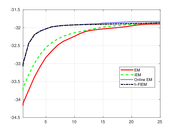
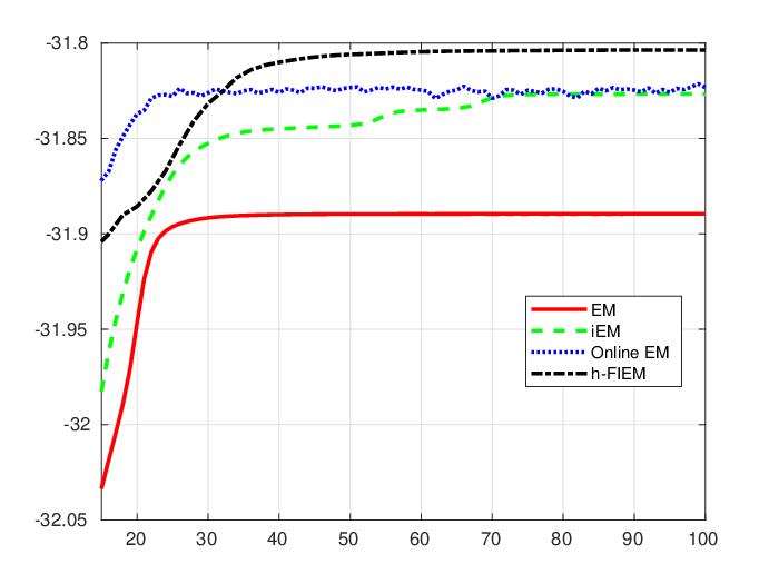
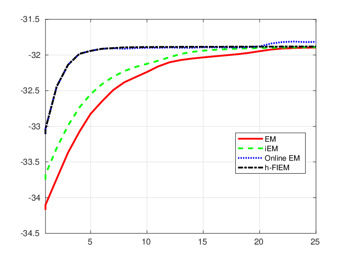
Figure 10and Figure 11 display the normalized log-likelihood along a path of EM, iEM, Online EM and h-FIEM, resp. for the first epochs (from $1$ to $25$ ) and by discarding the first ones (from $15$ to $100$ ). The first conclusion is that the incremental methods forget the initial value far more rapidly than EM, which is the consequence of the incremental processing of the observations which allow many updates of the parameter $\theta^{k}$ (or equivalently, of the statistic $\widehat{S}^{k}$ ) before the use of $n$ examples (which is equivalent to the learning cost of one iteration of EM). The second conclusion is that the incremental EM-based methods perform a better maximization of the normalized log-likelihood $-F$ . Finally, Online EM and h-FIEM are better than iEM: the log-likelihood converges resp. to $-1.9094\,\mathrm{e}{+6}$ , $-1.9080\,\mathrm{e}{+6}$ and $-1.9100\,\mathrm{e}{+6}$ (the plot displays the normalized log-likelihood); and it is clear that h-FIEM reduces the variability of the Online EM path. The same conclusions are drawn from different runs; the supplementary material provides a similar plot when the curves are the average over $10$ independent paths; Table 1 reports the mean value and the standard deviation of the log-likelihood over these $10$ runs.

Table 1: Normalized log-likelihood along a EM, iEM, Online EM and h-FIEM path, at epoch

\#1,15,25,50,100

. The value is the average over

10

independent runs (the standard deviation is in parenthesis). The log-likelihood is obtained by multiplying by

n=6\mathrm{e}{+4}

	$\#1$	$\#15$	$\#25$	$\#50$	$\#100$
EM	$-3.4102\mathrm{e}{+1}$	$-3.2033\mathrm{e}{+1}$	$-3.1896\mathrm{e}{+1}$	$-3.1890\mathrm{e}{+1}$	$-3.1889\mathrm{e}{+1}$
	-	-	-	-	-
iEM	$-3.3672\mathrm{e}{+1}$	$-3.1982\mathrm{e}{+1}$	$-3.1869\mathrm{e}{+1}$	$-3.1843\mathrm{e}{+1}$	$-3.1827\mathrm{e}{+1}$
	$(4.90\mathrm{e}{-3})$	$(5.33\mathrm{e}{-2})$	$(1.87\mathrm{e}{-2})$	$(1.87\mathrm{e}{-2})$	$(1.38\mathrm{e}{-2})$
Online EM	-3.2999 $\mathrm{e}{+1}$	-3.1872 $\mathrm{e}{+1}$	-3.1828 $\mathrm{e}{+1}$	$-3.1823\mathrm{e}{+1}$	$-3.1823\mathrm{e}{+1}$
	$(2.67\mathrm{e}{-2})$	$(5.14\mathrm{e}{-2})$	$(4.67\mathrm{e}{-2})$	$(4.68\mathrm{e}{-2})$	$(4.50\mathrm{e}{-2})$
h-FIEM	$-3.2999\mathrm{e}{+1}$	$-3.1900\mathrm{e}{+1}$	$-3.1853\mathrm{e}{+1}$	-3.1806 $\mathrm{e}{+1}$	-3.1804 $\mathrm{e}{+1}$
	$(2.67\mathrm{e}{-2})$	$(5.31\mathrm{e}{-2})$	$(6.94\mathrm{e}{-2})$	$(5.18\mathrm{e}{-2})$	$(5.25\mathrm{e}{-2})$

A fluctuation of $1\%$ (resp. $1$ ‰) around the optimal normalized log-likelihood corresponds to a lower bound of $-32.1184$ (resp. $-31.8322$ ): for EM such an accuracy is reached after $12$ iterations (resp. is never reached); for iEM, it is reached after $11$ epochs (resp. is never reached); for Online EM, after $4$ epochs (resp. $23$ epochs); for h-FIEM, after $4$ epochs (resp. $34$ epochs). An accuracy of $1$ ‱ is never reached by Online EM and is reached after $36$ epochs for h-FIEM.

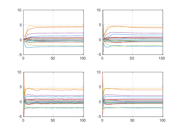
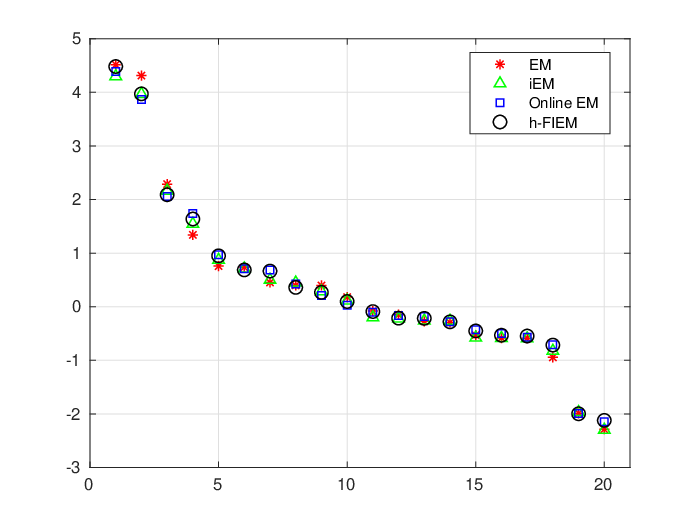
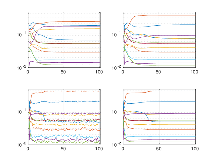
Figure 12shows the estimation of the $g=12$ weights $\alpha_{\ell}$ along a path of length $100$ epochs. The comparison of Online EM (bottom left) and h-FIEM (bottom right) shows that h-FIEM acts as a variability reduction technique along the path, without slowing down the convergence rate. Figure 13 displays the limiting value of these paths i.e. the estimate of the weights $\alpha_{1},\ldots,\alpha_{g}$ defined as the value of the parameter at the end of $100$ epochs; the weights are sorted in descending order. Online EM and h-FIEM provide similar estimates.

6 Proof

6.1 Proof of section 2

6.1.1 Proof of subsection 2.1

(Proof of 1).

The statements are trivial and we only prove the first claim: if $s^{\star}=\bar{s}\circ\mathsf{T}(s^{\star})$ then by applying $\mathsf{T}$ (under the uniqueness assumption A3), we have $\mathsf{T}(s^{\star})=(\mathsf{T}\circ\bar{s})\circ\mathsf{T}(s^{\star})$ and the proof follows.

(Proof of 2).

For $\theta\in\Theta^{v}$ , set $D\phi(\theta)\stackrel{{\scriptstyle\mathrm{def}}}{{=}}\left(\dot{\phi}(\theta)\right)^{T}$ . By A4-(ii) and a chain rule,

\dot{V}(s)=\left(\dot{\mathsf{T}}(s)\right)^{T}\ \left\{\dot{\mathsf{R}}(\mathsf{T}(s))-D\phi(\mathsf{T}(s))\ \bar{s}\circ\mathsf{T}(s)\right\}\;.

Moreover, using A3 and A4-(i), the minimum $\mathsf{T}(s)$ is a critical point of $\theta\mapsto\mathsf{L}(s,\theta)$ : we have for any $s\in{\mathbb{R}^{q}}$ , $\dot{\mathsf{R}}(\mathsf{T}(s))-D\phi(\mathsf{T}(s))\,s=0$ . Hence,

\dot{V}(s)=-\left(\dot{\mathsf{T}}(s)\right)^{T}\ D\phi(\mathsf{T}(s))\ h(s)=-\left(B(s)\right)^{T}\ h(s)\;.

A4-(iii) implies that $B^{T}=B$ and the zeros of $h$ are the zeros of $\dot{V}$ .

6.1.2 Auxiliary result

Lemma 7.

Assume that $\Theta$ and $\phi(\Theta)$ are open; and $\phi$ is continuously differentiable on $\Theta$ . Then for all $i\in\{1,\ldots,n\}$ , $\mathcal{L}_{i}$ is continuously differentiable on $\Theta$ .

If in addition A1, A2, A3 and A4-(i) hold, then $F$ (resp. $V\stackrel{{\scriptstyle\mathrm{def}}}{{=}}F\circ\mathsf{T}$ ) is continuously differentiable on $\Theta$ (resp. on ${\mathbb{R}^{q}}$ ) and for any $\theta\in\Theta$ ,

\dot{F}(\theta)=-\left(\dot{\phi}(\theta)\right)^{T}\,\bar{s}(\theta)+\dot{\mathsf{R}}(\theta)\;.

Proof.

A1 and (Sundberg 2019, Proposition 3.8) (see also (Brown 1986, Theorem 2.2.)) imply that $L_{i}:\tau\mapsto\int_{Z}h_{i}(z)\,\exp\left({\left\langle s_{i}(z),\tau\right\rangle}\right)\mu(\mathrm{d}z)$ is continuously differentiable on the interior of the set

\{\tau\in\mathbb{R}^{q},\int_{Z}h_{i}(z)\,\exp\left({\left\langle s_{i}(z),\tau\right\rangle}\right)\mu(\mathrm{d}z)<\infty\}

and its derivative is

\int_{\mathsf{Z}}s_{i}(z)\ h_{i}(z)\,\exp\left({\left\langle s_{i}(z),\tau\right\rangle}\right)\mu(\mathrm{d}z)\;.

This set contains $\phi(\Theta)$ under A1. The equality $\mathcal{L}_{i}=-\log(L_{i}\circ\phi)$ and the differentiability of composition of functions conclude the proof of the first item. The second one easily follows. ∎

6.2 Proofs of section 3

For any $k\geq 0$ and $i\in[n]^{\star}$ , we define $\widehat{S}^{<k,i}$ such that

\widetilde{S}^{k}=\frac{1}{n}\sum_{i=1}^{n}\bar{s}_{i}\circ\mathsf{T}(\widehat{S}^{<k,i})\;;

it means $\widehat{S}^{<0,i}\stackrel{{\scriptstyle\mathrm{def}}}{{=}}\widehat{S}^{0}$ for all $i\in[n]^{\star}$ and for $k\geq 0$ ,

(26)

\widehat{S}^{<k+1,i}=\widehat{S}^{\ell},

with

(27)

\left\{\begin{array}[]{ll}\ell=k&\text{if $I_{k+1}=i$,}\\ \ell\in[k-1]^{\star}&\text{if $I_{k+1}\neq i,I_{k}\neq i,\ldots,I_{\ell+1}=i$,}\\ \ell=0&\text{otherwise.}\end{array}\right.

Define the filtrations, for $k\geq 0$ ,

	$\displaystyle\mathcal{F}_{k}$	$\displaystyle\stackrel{{\scriptstyle\mathrm{def}}}{{=}}\sigma(\widehat{S}^{0},I_{1},J_{1},\ldots,I_{k},J_{k}),$
	$\displaystyle\mathcal{F}_{k+1/2}$	$\displaystyle\stackrel{{\scriptstyle\mathrm{def}}}{{=}}\sigma(\widehat{S}^{0},I_{1},J_{1},\ldots,I_{k},J_{k},I_{k+1})\;;$

note that $\widehat{S}^{k}\in\mathcal{F}_{k}$ and $\mathsf{S}_{k+1,\cdot}\in\mathcal{F}_{k+1/2}$ . Set

H_{k+1}\stackrel{{\scriptstyle\mathrm{def}}}{{=}}\bar{s}_{J_{k+1}}\circ\mathsf{T}(\widehat{S}^{k})-\widehat{S}^{k}+\frac{1}{n}\sum_{i=1}^{n}\mathsf{S}_{k+1,i}-\mathsf{S}_{k+1,J_{k+1}}\;.

6.2.1 Proof of Theorem 3

By subsection 2.1 and A5-(iii), $\dot{V}$ is $L_{\dot{V}}$ -Lipschitz on $\mathbb{R}^{q}$ , and we have

	$\displaystyle V(\widehat{S}^{k+1})-V(\widehat{S}^{k})$	$\displaystyle\leq\left\langle\widehat{S}^{k+1}-\widehat{S}^{k},\dot{V}(\widehat{S}^{k})\right\rangle+\frac{L_{\dot{V}}}{2}\\|\widehat{S}^{k+1}-\widehat{S}^{k}\\|^{2}$
		$\displaystyle\leq\gamma_{k+1}\left\langle H_{k+1},\dot{V}(\widehat{S}^{k})\right\rangle+\gamma_{k+1}^{2}\frac{L_{\dot{V}}}{2}\\|H_{k+1}\\|^{2}.$

Taking the expectation yields, upon noting that $\widehat{S}^{k}\in\mathcal{F}_{k}$ ,

		$\displaystyle\mathbb{E}\left[V(\widehat{S}^{k+1})\right]-\mathbb{E}\left[V(\widehat{S}^{k})\right]$
		$\displaystyle\leq\gamma_{k+1}\mathbb{E}\left[\left\langle\mathbb{E}\left[H_{k+1}\|\mathcal{F}_{k}\right],\dot{V}(\widehat{S}^{k})\right\rangle\right]+\gamma_{k+1}^{2}\frac{L_{\dot{V}}}{2}\mathbb{E}\left[\\|H_{k+1}\\|^{2}\right]$
		$\displaystyle\leq\gamma_{k+1}\mathbb{E}\left[\left\langle h(\widehat{S}^{k}),\dot{V}(\widehat{S}^{k})\right\rangle\right]+\gamma_{k+1}^{2}\frac{L_{\dot{V}}}{2}\mathbb{E}\left[\\|H_{k+1}\\|^{2}\right]$
		$\displaystyle\leq-\gamma_{k+1}v_{min}\mathbb{E}\left[\\|h(\widehat{S}^{k})\\|^{2}\right]+\gamma_{k+1}^{2}\frac{L_{\dot{V}}}{2}\mathbb{E}\left[\\|H_{k+1}\\|^{2}\right]$
		$\displaystyle\leq-\gamma_{k+1}\left(v_{min}-\gamma_{k+1}\frac{L_{\dot{V}}}{2}\right)\mathbb{E}\left[\\|h(\widehat{S}^{k})\\|^{2}\right]$
		$\displaystyle\qquad+\gamma_{k+1}^{2}\frac{L_{\dot{V}}}{2}\mathbb{E}\left[\\|H_{k+1}-h(\widehat{S}^{k})\\|^{2}\right]$

where we used that $\mathbb{E}\left[H_{k+1}|\mathcal{F}_{k}\right]=h(\widehat{S}^{k})$ and subsection 3.1. Set

	$\displaystyle A_{k}$	$\displaystyle\stackrel{{\scriptstyle\mathrm{def}}}{{=}}\mathbb{E}\left[\\|h(\widehat{S}^{k})\\|^{2}\right]\;,$
	$\displaystyle B_{k+1}$	$\displaystyle\stackrel{{\scriptstyle\mathrm{def}}}{{=}}\mathbb{E}\left[\\|\widetilde{S}^{k+1}-\bar{s}\circ\mathsf{T}(\widehat{S}^{k})\\|^{2}\right]\;.$

By subsubsection 6.2.5 and subsubsection 6.2.5, we have for any $k\geq 0$ :

	$\displaystyle\mathbb{E}\left[V(\widehat{S}^{k+1})\right]-\mathbb{E}\left[V(\widehat{S}^{k})\right]$	$\displaystyle\leq-\gamma_{k+1}\left(v_{min}-\gamma_{k+1}\frac{L_{\dot{V}}}{2}\right)A_{k}-\gamma_{k+1}^{2}\frac{L_{\dot{V}}}{2}B_{k+1}$
		$\displaystyle+\gamma_{k+1}^{2}\frac{L_{\dot{V}}}{2}\mathbb{E}\left[\\|\bar{s}_{J_{k+1}}\circ\mathsf{T}(\widehat{S}^{k})-\mathsf{S}_{k+1,J_{k+1}}\\|^{2}\right]$
		$\displaystyle\leq T_{1,k}+T_{2,k+1}$

by setting

	$\displaystyle T_{1,k}$	$\displaystyle\stackrel{{\scriptstyle\mathrm{def}}}{{=}}-\gamma_{k+1}\left(v_{min}-\gamma_{k+1}\frac{L_{\dot{V}}}{2}\right)A_{k}+\gamma_{k+1}^{2}\frac{L_{\dot{V}}}{2}\sum_{j=0}^{k-1}\tilde{\Lambda}_{j+1,k}A_{j}$
	$\displaystyle T_{2,k+1}$	$\displaystyle\stackrel{{\scriptstyle\mathrm{def}}}{{=}}-\gamma_{k+1}^{2}\frac{L_{\dot{V}}}{2}\left\{B_{k+1}+\sum_{j=0}^{k-1}\tilde{\Lambda}_{j+1,k}(1+\beta_{j+1}^{-1})^{-1}B_{j+1}\right\}\;;$

by convention, $\sum_{j=0}^{1}a_{j}=0$ . By summing from $k=0$ to $k=K_{\mathrm{max}}-1$ , we have

\sum_{k=0}^{K_{\mathrm{max}}-1}\gamma_{k+1}\left(v_{min}-\gamma_{k+1}\frac{L_{\dot{V}}}{2}\right)A_{k}-\frac{L_{\dot{V}}\,L^{2}}{2}\sum_{k=0}^{K_{\mathrm{max}}-2}\gamma_{k+1}^{2}\Lambda_{k}\ A_{k}\\ \leq\Delta V-\frac{L_{\dot{V}}}{2}\sum_{k=0}^{K_{\mathrm{max}}-1}\gamma_{k+1}^{2}\left(L^{2}\Xi_{k}+1\right)B_{k+1},

where for $0\leq k\leq K_{\mathrm{max}}-2$ and with the convention $\Lambda_{K_{\mathrm{max}}-1}=\Xi_{K_{\mathrm{max}}-1}=0$ ,

	$\displaystyle\Lambda_{k}$	$\displaystyle\stackrel{{\scriptstyle\mathrm{def}}}{{=}}\left(1+\frac{1}{\beta_{k+1}}\right)\ \sum_{j=k+1}^{K_{\mathrm{max}}-1}\gamma_{j+1}^{2}\ \left(\frac{n-1}{n}\right)^{j-k}\ \prod_{\ell=k+2}^{j}\left(1+\beta_{\ell}+\gamma_{\ell}^{2}L^{2}\right)$
		$\displaystyle\leq\left(1+\frac{1}{\beta_{k+1}}\right)\ \sum_{j=k+1}^{K_{\mathrm{max}}-1}\gamma_{j+1}^{2}\ \prod_{\ell=k+2}^{j}\left(1-\frac{1}{n}+\beta_{\ell}+\gamma_{\ell}^{2}L^{2}\right),$
	$\displaystyle\Xi_{k}$	$\displaystyle\stackrel{{\scriptstyle\mathrm{def}}}{{=}}\left(1+\frac{1}{\beta_{k+1}}\right)^{-1}\Lambda_{k}=\frac{\Lambda_{k}\beta_{k+1}}{1+\beta_{k+1}}\;.$

Hence,

\sum_{k=0}^{K_{\mathrm{max}}-1}\{\gamma_{k+1}\left(v_{min}-\gamma_{k+1}\frac{L_{\dot{V}}}{2}\right)-\gamma_{k+1}^{2}\Lambda_{k}\frac{L_{\dot{V}}L^{2}}{2}\}\ A_{k}\\ +\sum_{k=0}^{K_{\mathrm{max}}-1}\gamma_{k+1}^{2}\{1+\Xi_{k}L^{2}\}\frac{L_{\dot{V}}}{2}B_{k+1}\leq\Delta V\;.

6.2.2 Proof of subsection 3.2

It is a follow-up of Theorem 3; the quantities $\alpha_{k},\Lambda_{k},\delta_{k}$ introduced in the statement of Theorem 3 are used below without being defined again. We consider the case when for $\ell\in[K_{\mathrm{max}}]^{\star}$ ,

\beta_{\ell}\stackrel{{\scriptstyle\mathrm{def}}}{{=}}\frac{1-\lambda}{n^{\mathsf{b}}}\;,\qquad\gamma_{\ell}^{2}\stackrel{{\scriptstyle\mathrm{def}}}{{=}}\frac{C}{L^{2}n^{2\mathsf{c}}K_{\mathrm{max}}^{2\mathsf{d}}}\;,

for some $\lambda\in\left(0,1\right)$ , $C>0$ and $\mathsf{b},\mathsf{c},\mathsf{d}$ to be defined in the proof in such a way that (i) $\alpha_{k}\geq 0$ , (ii) $\sum_{k=0}^{K_{\mathrm{max}}-1}\alpha_{k}$ is positive and as large as possible. Since there will be a discussion on $(n,C,\lambda)$ , we make more explicit the dependence of some constants upon these quantities: $\alpha_{k}$ will be denoted by $\alpha_{k}(n,C,\lambda)$ .

With these definitions, we have

\displaystyle 1-\frac{\rho_{n}}{n}

\displaystyle\stackrel{{\scriptstyle\mathrm{def}}}{{=}}1-\frac{1}{n}+\beta_{\ell}+\gamma_{\ell}^{2}L^{2}=1-\frac{1}{n}\left(1-\frac{1-\lambda}{n^{\mathsf{b}-1}}-\frac{C}{n^{2\mathsf{c}-1}K_{\mathrm{max}}^{2\mathsf{d}}}\right)\;,

and choose $(\mathsf{b},\mathsf{c},\mathsf{d},\lambda,C)$ such that

(28)

\frac{1-\lambda}{n^{\mathsf{b}-1}}+\frac{C}{n^{2\mathsf{c}-1}K_{\mathrm{max}}^{2\mathsf{d}}}<1\;,

which ensures that $\rho_{n}\in\left(0,1\right)$ . Hence, for any $k\in[K_{\mathrm{max}}-2]$ ,

	$\displaystyle\Lambda_{k}$	$\displaystyle\leq n^{\mathsf{b}}\left(\frac{1}{n^{\mathsf{b}}}+\frac{1}{1-\lambda}\right)\frac{C}{L^{2}n^{2\mathsf{c}}K_{\mathrm{max}}^{2\mathsf{d}}}\sum_{j=k+1}^{K_{\mathrm{max}}-1}\left(1-\frac{\rho_{n}}{n}\right)^{j-k-1}$
		$\displaystyle\leq\left(\frac{1}{n^{\mathsf{b}}}+\frac{1}{1-\lambda}\right)\frac{C}{L^{2}\rho_{n}}\frac{1}{n^{2\mathsf{c}-\mathsf{b}-1}K_{\mathrm{max}}^{2\mathsf{d}}}\;.$

From this upper bound, we deduce for any $k\in[K_{\mathrm{max}}-1]$ : $\alpha_{k}(n,C,\lambda)\geq\underline{\alpha}_{n}(C,\lambda)$ where

(29)

\displaystyle\underline{\alpha}_{n}(C,\lambda)\stackrel{{\scriptstyle\mathrm{def}}}{{=}}\frac{\sqrt{C}}{Ln^{\mathsf{c}}K_{\mathrm{max}}^{\mathsf{d}}}\left(v_{\mathrm{min}}-\frac{L_{\dot{V}}}{2L}\frac{\sqrt{C}}{n^{\mathsf{c}}K_{\mathrm{max}}^{\mathsf{d}}}-\frac{L_{\dot{V}}}{2L}\frac{C^{3/2}}{\rho_{n}\,n^{3\mathsf{c}-\mathsf{b}-1}K_{\mathrm{max}}^{3\mathsf{d}}}\left(\frac{1}{n^{\mathsf{b}}}+\frac{1}{1-\lambda}\right)\right)\;.

From (28) and (29), we choose $\mathsf{b}=1$ , $\mathsf{c}=2/3$ , $\mathsf{d}=0$ ; which yields for $n\geq 1$ , since $\rho_{n}=\lambda-Cn^{-1/3}$

n^{2/3}\underline{\alpha}_{n}(C,\lambda)\geq\mathcal{L}_{n}(C,\lambda)\;,

with

	$\displaystyle\mathcal{L}_{n}(C,\lambda)$	$\displaystyle\stackrel{{\scriptstyle\mathrm{def}}}{{=}}\frac{L_{\dot{V}}\sqrt{C}}{2L^{2}}\left(v_{\mathrm{min}}\frac{2L}{L_{\dot{V}}}-\sqrt{C}f_{n}(C,\lambda)\right)\;,$
	$\displaystyle f_{n}(C,\lambda)$	$\displaystyle\stackrel{{\scriptstyle\mathrm{def}}}{{=}}\frac{1}{n^{2/3}}+\frac{C}{\lambda-Cn^{-1/3}}\left(\frac{1}{n}+\frac{1}{1-\lambda}\right)\;.$

Let $\mu\in\left(0,1\right)$ . Fix $\lambda\in\left(0,1\right)$ and $C>0$ such that (see (28) for the second condition)

(30)

\sqrt{C}f_{n}(C,\lambda)=2\mu v_{\mathrm{min}}\frac{L}{L_{\dot{V}}}\;,\qquad\frac{1}{n^{1/3}}<\frac{\lambda}{C}\;.

This implies that $n^{2/3}\alpha_{k}(n,C,\lambda)\geq n^{2/3}\underline{\alpha}_{n}(C,\lambda)\geq n^{2/3}\alpha_{\star}(C)\stackrel{{\scriptstyle\mathrm{def}}}{{=}}\sqrt{C}(1-\mu)v_{\mathrm{min}}/L$ . We obtain an upper bound on $\mathsf{E}_{1}$ by

\mathsf{E}_{1}\leq\frac{1}{K_{\mathrm{max}}\ \alpha_{\star}(C)}\sum_{k=0}^{K_{\mathrm{max}}-1}\alpha_{k}(n,C,\lambda)\,\mathbb{E}\left[\|h(\widehat{S}^{k})\|^{2}\right]\;.

For $\mathsf{E}_{2}$ , since $\delta_{k}\geq L_{\dot{V}}\gamma_{k+1}^{2}/2$ ,

\frac{L_{\dot{V}}\,\sqrt{C}}{2L(1-\mu)n^{2/3}}\frac{1}{v_{\mathrm{min}}}\mathsf{E}_{2}\\ \leq\frac{L_{\dot{V}}\,C}{2L^{2}n^{4/3}}\frac{1}{K_{\mathrm{max}}\ \alpha_{\star}(C)}\sum_{k=0}^{K_{\mathrm{max}}-1}\mathbb{E}\left[\|\widetilde{S}^{k+1}-\bar{s}\circ\mathsf{T}(\widehat{S}^{k})\|^{2}\right]\\ \leq\frac{1}{K_{\mathrm{max}}\ \alpha_{\star}(C)}\sum_{k=0}^{K_{\mathrm{max}}-1}\delta_{k}\mathbb{E}\left[\|\widetilde{S}^{k+1}-\bar{s}\circ\mathsf{T}(\widehat{S}^{k})\|^{2}\right]\;.

We then conclude by

(31)

\frac{1}{K_{\mathrm{max}}\,\alpha_{\star}(C)}=\frac{n^{2/3}}{K_{\mathrm{max}}}\frac{L}{\sqrt{C}(1-\mu)v_{\mathrm{min}}}\;,

and use $\sqrt{C}f_{n}(C,\lambda)=2\mu v_{\mathrm{min}}L/L_{\dot{V}}$ .

6.2.3 Proof of subsection 3.3

It is a follow-up of Theorem 3; the quantities $\alpha_{k},\Lambda_{k},\delta_{k}$ introduced in the statement of Theorem 3 are used below without being defined again.

We consider the case when, for $\ell\in[K_{\mathrm{max}}]^{\star}$ ,

\beta_{\ell}\stackrel{{\scriptstyle\mathrm{def}}}{{=}}\frac{1-\lambda}{n^{\mathsf{b}}},\qquad\gamma_{\ell}^{2}\stackrel{{\scriptstyle\mathrm{def}}}{{=}}\frac{C}{L^{2}n^{2\mathsf{c}}K_{\mathrm{max}}^{2\mathsf{d}}}

With these definitions, we have

\rho\stackrel{{\scriptstyle\mathrm{def}}}{{=}}1-\frac{1}{n}+\beta_{\ell}+L^{2}\gamma_{\ell}^{2}=1-\frac{1}{n}\left(1-\frac{1-\lambda}{n^{\mathsf{b}-1}}-\frac{C}{n^{2\mathsf{c}-1}K_{\mathrm{max}}^{2\mathsf{d}}}\right)\;,

and choose $(\mathsf{b},\mathsf{c},\mathsf{d},\lambda,C)$ such that

(32)

\frac{1-\lambda}{n^{\mathsf{b}-1}}+\frac{C}{n^{2\mathsf{c}-1}K_{\mathrm{max}}^{2\mathsf{d}}}\leq 1\;,

which ensures that $\rho\in\left(0,1\right]$ . Hence, for any $k\in[K_{\mathrm{max}}-2]$ ,

	$\displaystyle\Lambda_{k}$	$\displaystyle\leq n^{\mathsf{b}}\left(\frac{1}{n^{\mathsf{b}}}+\frac{1}{1-\lambda}\right)\frac{C}{L^{2}n^{2\mathsf{c}}K_{\mathrm{max}}^{2\mathsf{d}}}\sum_{j=k+1}^{K_{\mathrm{max}}-1}\rho^{j-k-1}$
		$\displaystyle\leq\left(\frac{1}{n^{\mathsf{b}}}+\frac{1}{1-\lambda}\right)\frac{C}{L^{2}n^{2\mathsf{c}-\mathsf{b}}K_{\mathrm{max}}^{2\mathsf{d}-1}}\;.$

From this upper bound, we obtain the following lower bound for any $k\in[K_{\mathrm{max}}-1]$ : $\alpha_{k}(n,C,\lambda)\geq\underline{\alpha}_{n}(C,\lambda)$ where

(n^{\mathsf{c}}K_{\mathrm{max}}^{\mathsf{d}})\ \underline{\alpha}_{n}(C,\lambda)\stackrel{{\scriptstyle\mathrm{def}}}{{=}}\frac{\sqrt{C}}{L}\left(v_{\mathrm{min}}-\sqrt{C}\frac{L_{\dot{V}}}{2L}\left\{\frac{1}{n^{\mathsf{c}}K_{\mathrm{max}}^{\mathsf{d}}}\right.\right.\\ \left.\left.+\frac{C}{n^{3\mathsf{c}-\mathsf{b}}K_{\mathrm{max}}^{3\mathsf{d}-1}}\left(\frac{1}{n^{\mathsf{b}}}+\frac{1}{1-\lambda}\right)\right\}\right)\;.

Based on this inequality and on (32), we choose $\mathsf{b}=1$ and $\mathsf{c}=\mathsf{d}=1/3$ ; which yields for $n\geq 1$ ,

		$\displaystyle(nK_{\mathrm{max}})^{1/3}\ \underline{\alpha}_{n}(C,\lambda)=\mathcal{L}_{n}(C,\lambda)\stackrel{{\scriptstyle\mathrm{def}}}{{=}}\frac{\sqrt{C}L_{\dot{V}}}{2L^{2}}\left(v_{\mathrm{min}}\frac{2L}{L_{\dot{V}}}-\sqrt{C}\tilde{f}_{n}(C,\lambda)\right)\;,$
		$\displaystyle\tilde{f}_{n}(C,\lambda)\stackrel{{\scriptstyle\mathrm{def}}}{{=}}\frac{1}{(nK_{\mathrm{max}})^{1/3}}+C\left(\frac{1}{n}+\frac{1}{1-\lambda}\right)\;.$

Let $\mu\in\left(0,1\right)$ . Fix $\lambda\in\left(0,1\right)$ and $C>0$ such that (see (32) for the second condition)

(33)

\sqrt{C}\tilde{f}_{n}(C,\lambda)=2\mu v_{\mathrm{min}}\frac{L}{L_{\dot{V}}}\;,\qquad\frac{n^{1/3}}{K_{\mathrm{max}}^{2/3}}\leq\frac{\lambda}{C}\;.

This implies that

(nK_{\mathrm{max}})^{1/3}\alpha_{k}(n,C,\lambda)\geq(nK_{\mathrm{max}})^{1/3}\underline{\alpha}_{n}(C,\lambda)\\ \geq(nK_{\mathrm{max}})^{1/3}\alpha_{\star}(C)\stackrel{{\scriptstyle\mathrm{def}}}{{=}}\sqrt{C}(1-\mu)v_{\mathrm{min}}/L\;.

We obtain the upper bound on $\mathsf{E}_{1}$ by

\mathsf{E}_{1}\leq\frac{1}{K_{\mathrm{max}}\ \alpha_{\star}(C)}\sum_{k=0}^{K_{\mathrm{max}}-1}\alpha_{k}(n,C,\lambda)\ \mathbb{E}\left[\|h(\widehat{S}^{k})\|^{2}\right]\;.

For $\mathsf{E}_{2}$ and since $\delta_{k}\geq L_{\dot{V}}\gamma_{k+1}^{2}/2$

\frac{L_{\dot{V}}\,\sqrt{C}}{2(1-\mu)Ln^{1/3}}\frac{1}{K_{\mathrm{max}}^{1/3}v_{\mathrm{min}}}\mathsf{E}_{2}\leq\frac{L_{\dot{V}}\,C}{2L^{2}n^{2/3}K_{\mathrm{max}}^{2/3}}\frac{1}{K_{\mathrm{max}}\ \alpha_{\star}(C)}\ \sum_{k=0}^{K_{\mathrm{max}}-1}\mathbb{E}\left[\|\widetilde{S}^{k+1}-\bar{s}\circ\mathsf{T}(\widehat{S}^{k})\|^{2}\right]\\ \leq\frac{1}{K_{\mathrm{max}}\ \alpha_{\star}(C)}\sum_{k=0}^{K_{\mathrm{max}}-1}\delta_{k}\mathbb{E}\left[\|\widetilde{S}^{k+1}-\bar{s}\circ\mathsf{T}(\widehat{S}^{k})\|^{2}\right]\;.

We then conclude by

(34)

\frac{1}{K_{\mathrm{max}}\alpha_{\star}(C)}=\frac{n^{1/3}}{K_{\mathrm{max}}^{2/3}}\frac{L}{\sqrt{C}(1-\mu)v_{\mathrm{min}}}\;,

and use $\sqrt{C}\tilde{f}_{n}(C,\lambda)=2\mu v_{\mathrm{min}}L/L_{\dot{V}}$ .

6.2.4 Proof of subsection 3.4

It is a follow-up of Theorem 3; the quantities $\alpha_{k},\Lambda_{k},\delta_{k}$ introduced in the statement of Theorem 3 are used below without being defined again.

Let $p_{0},\ldots,p_{K_{\mathrm{max}}-1}$ be positive real numbers such that $\sum_{k=0}^{K_{\mathrm{max}}-1}p_{k}=1$ . We consider the case when

\beta_{\ell}\stackrel{{\scriptstyle\mathrm{def}}}{{=}}\frac{1-\lambda}{n^{\mathsf{b}}}\;,\qquad\gamma_{\ell}^{2}\stackrel{{\scriptstyle\mathrm{def}}}{{=}}\frac{C_{\ell}}{L^{2}n^{2\mathsf{c}}K_{\mathrm{max}}^{2\mathsf{d}}}\;,

for $\lambda\in\left(0,1\right)$ , $C_{\ell}>0$ , and $\mathsf{b},\mathsf{c},\mathsf{d}$ to be defined in the proof.

The first step consists in the definition of a function $\mathcal{A}$ and of a family $\mathcal{C}$ of vectors $\underline{C}=(C_{1},\ldots,C_{K_{\mathrm{max}}})\in(\mathbb{R}^{+})^{K_{\mathrm{max}}}$ such that

\alpha_{k}\geq\mathcal{A}(C_{k+1})\geq 0\;,\qquad\sum_{\ell=0}^{K_{\mathrm{max}}-1}\mathcal{A}(C_{\ell+1})>0\;.

The second step proves that we can find $\underline{C}\in\mathcal{C}$ such that $p_{k}=\mathcal{A}(C_{k+1})/\sum_{\ell=0}^{K_{\mathrm{max}}-1}\mathcal{A}(C_{\ell+1})$ for any $k\in[K_{\mathrm{max}}-1]$ .

Such a pair $(\mathcal{A},\underline{C})$ is not unique, and among the possible ones, we indicate two strategies, all motivated by making the sum $\sum_{\ell=0}^{K_{\mathrm{max}}-1}\mathcal{A}(C_{\ell+1})$ as large as possible.

Step 1- Definition of the function $\mathcal{A}$ . With the definition of the sequences $\gamma_{\ell}$ and $\beta_{\ell}$ , we have

1-\frac{\rho_{n,\ell}}{n}\stackrel{{\scriptstyle\mathrm{def}}}{{=}}1-\frac{1}{n}+\beta_{\ell}+\gamma_{\ell}^{2}L^{2}=-\frac{1}{n}\left(1-\frac{1-\lambda}{n^{\mathsf{b}-1}}-\frac{C_{\ell}}{n^{2\mathsf{c}-1}K_{\mathrm{max}}^{2\mathsf{d}}}\right)

and choose $(\mathsf{b},\mathsf{c},\mathsf{d},\lambda,C_{\ell})$ such that

(35)

\frac{1-\lambda}{n^{\mathsf{b}-1}}+\frac{C_{\mathrm{max}}}{n^{2\mathsf{c}-1}K_{\mathrm{max}}^{2\mathsf{d}}}<1\;,\ \text{where}\ C_{\mathrm{max}}\stackrel{{\scriptstyle\mathrm{def}}}{{=}}\mathrm{max}_{\ell}C_{\ell}\;,

which ensures that $\rho_{n,\ell}\in\left(0,1\right)$ . Define

\rho_{n}\stackrel{{\scriptstyle\mathrm{def}}}{{=}}\mathrm{min}_{\ell}\rho_{n,\ell}=1-\frac{1-\lambda}{n^{\mathsf{b}-1}}-\frac{C_{\mathrm{max}}}{n^{2\mathsf{c}-1}K_{\mathrm{max}}^{2\mathsf{d}}}\;.

Hence, for any $k\in[K_{\mathrm{max}}-2]$ ,

	$\displaystyle\Lambda_{k}$	$\displaystyle\leq n^{\mathsf{b}}\left(\frac{1}{n^{\mathsf{b}}}+\frac{1}{1-\lambda}\right)\frac{1}{L^{2}n^{2\mathsf{c}}K_{\mathrm{max}}^{2\mathsf{d}}}\sum_{j=k+1}^{K_{\mathrm{max}}-1}C_{j+1}\left(1-\frac{\rho_{n}}{n}\right)^{j-k-1}$
		$\displaystyle\leq\left(\frac{1}{n^{\mathsf{b}}}+\frac{1}{1-\lambda}\right)\frac{C_{\mathrm{max}}}{L^{2}\rho_{n}}\frac{1}{n^{2\mathsf{c}-\mathsf{b}-1}K_{\mathrm{max}}^{2\mathsf{d}}}\;.$

From this upper bound, we obtain the following lower bound on $\alpha_{k}$ , for any $k\in[K_{\mathrm{max}}-1]$ ,

\alpha_{k}\geq\frac{\sqrt{C_{k+1}}}{Ln^{\mathsf{c}}K_{\mathrm{max}}^{\mathsf{d}}}\left(v_{\mathrm{min}}-\frac{L_{\dot{V}}}{2L}\frac{\sqrt{C_{k+1}}}{n^{\mathsf{c}}K_{\mathrm{max}}^{\mathsf{d}}}-\frac{L_{\dot{V}}}{2L}\frac{C_{\mathrm{max}}\sqrt{C_{k+1}}}{\rho_{n}\,n^{3\mathsf{c}-\mathsf{b}-1}K_{\mathrm{max}}^{3\mathsf{d}}}\left(\frac{1}{n^{\mathsf{b}}}+\frac{1}{1-\lambda}\right)\right)\;.

Based on this inequality and on (35), we choose $\mathsf{b}=1$ , $\mathsf{c}=2/3$ , $\mathsf{d}=0$ : this yields $\rho_{n}=\lambda-C_{\mathrm{max}}n^{-1/3}$ and $\alpha_{k}\geq\underline{\alpha}_{k}$ with (see (16) for the definition of $f_{n}$ )

(36)

\underline{\alpha}_{k}\stackrel{{\scriptstyle\mathrm{def}}}{{=}}\frac{\sqrt{C_{k+1}}L_{\dot{V}}}{2L^{2}n^{2/3}}\left(v_{\mathrm{min}}\frac{2L}{L_{\dot{V}}}-\sqrt{C_{k+1}}f_{n}(C_{\mathrm{max}},\lambda)\right)\;;

the condition (35) gets into $n^{-1/3}<\lambda/C_{\mathrm{max}}$ .

Define the quadratic function $x\mapsto\mathcal{A}(x)\stackrel{{\scriptstyle\mathrm{def}}}{{=}}Ax(v_{\mathrm{min}}-Bx)$ where

(37)

A\stackrel{{\scriptstyle\mathrm{def}}}{{=}}\frac{1}{Ln^{2/3}}\;,\quad B\stackrel{{\scriptstyle\mathrm{def}}}{{=}}f_{n}(C,\lambda)\frac{L_{\dot{V}}}{2L}\;;

we have $\underline{\alpha}_{k}=\mathcal{A}(\sqrt{C_{k+1}})$ . By section 9 in the supplementary material, $\mathcal{A}$ is increasing on $\left(0,v_{\mathrm{min}}/(2B)\right]$ , reaches its maximum at $x_{\star}\stackrel{{\scriptstyle\mathrm{def}}}{{=}}v_{\mathrm{min}}/(2B)$ and its maximal value is $\mathcal{A}_{\star}\stackrel{{\scriptstyle\mathrm{def}}}{{=}}Av^{2}_{\mathrm{min}}/(4B)$ . In addition, its inverse $\mathcal{A}^{-1}$ exists on $\left(0,\mathcal{A}_{\star}\right]$ .

Step 2- Choice of $C_{1},\ldots,C_{K_{\mathrm{max}}}$ . We are now looking for $C_{1},\ldots,C_{K_{\mathrm{max}}}$ such that

p_{k}=\mathcal{A}(\sqrt{C_{k+1}})/\sum_{\ell=0}^{K_{\mathrm{max}}-1}\mathcal{A}(\sqrt{C_{\ell+1}})

or equivalently

(38)

\frac{p_{k}}{p_{I}}=\frac{\mathcal{A}(\sqrt{C_{k+1}})}{\mathcal{A}(\sqrt{C_{I}})},\qquad I\in\mathrm{argmax}_{k}p_{k}\;.

It remains to fix $\mathcal{A}(\sqrt{C_{I}})$ in such a way that $\mathcal{A}$ is invertible on $\left(0,\sqrt{C_{I}}\right]$ . Since we also want $\sum_{\ell}\mathcal{A}(\sqrt{C_{\ell+1}})=\mathcal{A}(\sqrt{C_{I}})/p_{I}$ as large as possible, and $\mathcal{A}$ is increasing on $\left(0,x_{\star}\right]$ , we choose

(39)

\sqrt{C_{I}}=\sqrt{C_{\mathrm{max}}}=x_{\star}=\frac{v_{\mathrm{min}}}{2B}\;.

Therefore, $C_{\mathrm{max}}$ solves the equation $\sqrt{C_{\mathrm{max}}}=v_{\mathrm{min}}/(2B)$ or equivalently

(40)

\frac{v_{\mathrm{min}}L}{L_{\dot{V}}}=\sqrt{C_{\mathrm{max}}}f_{n}(C_{\mathrm{max}},\lambda)\;,

under the constraint that $\lambda\in\left(0,1\right)$ and $n^{-1/3}<\lambda/C_{\mathrm{max}}$ . When $C_{\mathrm{max}}$ is fixed, we set

\sqrt{C_{k+1}}\stackrel{{\scriptstyle\mathrm{def}}}{{=}}\mathcal{A}^{-1}\left(\frac{p_{k}}{\mathrm{max}_{\ell}p_{l}}\mathcal{A}(\sqrt{C_{\mathrm{max}}})\right).

With these definitions, we have (see (38))

\frac{1}{\sum_{k=0}^{K_{\mathrm{max}}-1}\mathcal{A}(\sqrt{C_{k+1}})}=\frac{\mathrm{max}_{\ell}p_{\ell}}{\mathcal{A}(\sqrt{C_{\mathrm{max}}})}.

Remember that

\mathcal{A}(\sqrt{C_{\mathrm{max}}})=\mathcal{A}(x_{\star})=v_{\mathrm{min}}\sqrt{C_{\mathrm{max}}}/(2Ln^{2/3})\;.

Step 3. Lower bound on $\delta_{k}$ We write

\delta_{k}\geq\frac{L_{\dot{V}}}{2}\gamma_{k+1}^{2}\;,

so that

\frac{\delta_{k}}{\sum_{k=0}^{K_{\mathrm{max}}-1}\mathcal{A}(\sqrt{C_{k+1}})}\geq\frac{L_{\dot{V}}L}{v_{\mathrm{min}}}n^{2/3}\frac{\mathrm{max}_{\ell}p_{\ell}}{\sqrt{C_{\mathrm{max}}}}\gamma_{k+1}^{2}\;.

6.2.5 Auxiliary results

Lemma 8.

Assume A1, A2 and A3. For any $k\geq 0$ ,

\mathbb{E}\left[\|H_{k+1}\|^{2}\right]=\mathbb{E}\left[\|H_{k+1}-h(\widehat{S}^{k})\|^{2}\right]+\mathbb{E}\left[\|h(\widehat{S}^{k})\|^{2}\right],

and

\mathbb{E}\left[\|H_{k+1}-h(\widehat{S}^{k})\|^{2}\right]+\mathbb{E}\left[\|\widetilde{S}^{k+1}-\bar{s}\circ\mathsf{T}(\widehat{S}^{k})\|^{2}\right]\\ =\mathbb{E}\left[\|\bar{s}_{J_{k+1}}\circ\mathsf{T}(\widehat{S}^{k})-\mathsf{S}_{k+1,J_{k+1}}\|^{2}\right]\;.

Proof.

Since $\mathbb{E}\left[H_{k+1}\big|\mathcal{F}_{k+1/2}\right]=h(\widehat{S}^{k})$ , we have

\displaystyle\mathbb{E}\left[\|H_{k+1}\|^{2}\right]

\displaystyle=\mathbb{E}\left[\|H_{k+1}-h(\widehat{S}^{k})\|^{2}\right]+\mathbb{E}\left[\|h(\widehat{S}^{k})\|^{2}\right]\;.

In addition, upon noting that $\mathsf{S}_{k+1,i}\in\mathcal{F}_{k+1/2}$ for any $i\in[n]^{\star}$ ,

	$\displaystyle H_{k+1}-h(\widehat{S}^{k})$	$\displaystyle=\bar{s}_{J_{k+1}}\circ\mathsf{T}(\widehat{S}^{k})-\mathsf{S}_{k+1,J_{k+1}}-\bar{s}\circ\mathsf{T}(\widehat{S}^{k})+\widetilde{S}^{k+1}$
		$\displaystyle=\bar{s}_{J_{k+1}}\circ\mathsf{T}(\widehat{S}^{k})-\mathsf{S}_{k+1,J_{k+1}}-\mathbb{E}\left[\bar{s}_{J_{k+1}}\circ\mathsf{T}(\widehat{S}^{k})-\mathsf{S}_{k+1,J_{k+1}}\Big\|\mathcal{F}_{k+1/2}\right]\;,$

we have

\mathbb{E}\left[\|H_{k+1}-h(\widehat{S}^{k})\|^{2}\right]+\mathbb{E}\left[\|\widetilde{S}^{k+1}-\bar{s}\circ\mathsf{T}(\widehat{S}^{k})\|^{2}\right]\\ =\mathbb{E}\left[\|\bar{s}_{J_{k+1}}\circ\mathsf{T}(\widehat{S}^{k})-\mathsf{S}_{k+1,J_{k+1}}\|^{2}\right]\;.

∎

Proposition 9.

Assume A1, A2, A3 and A5-(ii). Set $L^{2}\stackrel{{\scriptstyle\mathrm{def}}}{{=}}n^{-1}\sum_{i=1}^{n}L_{i}^{2}$ . Then

\mathbb{E}\left[\|\bar{s}_{J_{1}}\circ\mathsf{T}(\widehat{S}^{0})-\mathsf{S}_{1,J_{1}}\|^{2}\right]=0\;,

and for any $k\geq 1$ and $\beta_{1},\ldots,\beta_{k}>0$ ,

\mathbb{E}\left[\|\bar{s}_{J_{k+1}}\circ\mathsf{T}(\widehat{S}^{k})-\mathsf{S}_{k+1,J_{k+1}}\|^{2}\right]\\ \leq\sum_{j=1}^{k}\widetilde{\Lambda}_{j,k}\left\{\ \mathbb{E}\left[\|h(\widehat{S}^{j-1})\|^{2}\right]-\left(1+\frac{1}{\beta_{j}}\right)^{-1}\mathbb{E}\left[\|\widetilde{S}^{j}-\bar{s}\circ\mathsf{T}(\widehat{S}^{j-1})\|^{2}\right]\right\}\;,

where

\displaystyle\widetilde{\Lambda}_{j,k}

\displaystyle\stackrel{{\scriptstyle\mathrm{def}}}{{=}}L^{2}\,\left(\frac{n-1}{n}\right)^{k-j+1}\gamma_{j}^{2}\left(1+\frac{1}{\beta_{j}}\right)\ \prod_{\ell=j+1}^{k}\left(1+\beta_{\ell}+\gamma_{\ell}^{2}L^{2}\right).

By convention, $\prod_{\ell=k+1}^{k}a_{\ell}=1$ .

Proof.

\displaystyle\mathbb{E}\left[\|\bar{s}_{J_{1}}\circ\mathsf{T}(\widehat{S}^{0})-\mathsf{S}_{1,J_{1}}\|^{2}\right]=\frac{1}{n}\sum_{i=1}^{n}\mathbb{E}\left[\|\bar{s}_{i}\circ\mathsf{T}(\widehat{S}^{0})-\mathsf{S}_{1,i}\|^{2}\right]=0\;.

Let $k\geq 1$ . We write (see (10))

\mathsf{S}_{k+1,i}=\mathsf{S}_{k,i}\mathbbm{1}_{I_{k+1}\neq i}+\bar{s}_{i}\circ\mathsf{T}(\widehat{S}^{k})\mathbbm{1}_{I_{k+1}=i}\\ =\bar{s}_{i}\circ\mathsf{T}(\widehat{S}^{<k,i})\mathbbm{1}_{I_{k+1}\neq i}+\bar{s}_{i}\circ\mathsf{T}(\widehat{S}^{k})\mathbbm{1}_{I_{k+1}=i},

where $\widehat{S}^{<\ell,i}$ is defined by (26). This yields, by A5-(ii)

	$\displaystyle\frac{1}{n}\sum_{i=1}^{n}\mathbb{E}\left[\\|\bar{s}_{i}\circ\mathsf{T}(\widehat{S}^{k})-\mathsf{S}_{k+1,i}\\|^{2}\right]$	$\displaystyle=\frac{1}{n}\sum_{i=1}^{n}\mathbb{E}\left[\\|\bar{s}_{i}\circ\mathsf{T}(\widehat{S}^{k})-\bar{s}_{i}\circ\mathsf{T}(\widehat{S}^{<k,i})\\|^{2}\mathbbm{1}_{I_{k+1}\neq i}\right]$
(41)			$\displaystyle\leq\Delta_{k}\stackrel{{\scriptstyle\mathrm{def}}}{{=}}\frac{n-1}{n^{2}}\sum_{i=1}^{n}L_{i}^{2}\,\mathbb{E}\left[\\|\widehat{S}^{k}-\widehat{S}^{<k,i}\\|^{2}\right].$

We have

\Delta_{k}=\frac{n-1}{n^{2}}\sum_{i=1}^{n}L_{i}^{2}\,\mathbb{E}\left[\|\widehat{S}^{k}-\widehat{S}^{k-1}+\left(\widehat{S}^{k-1}-\widehat{S}^{<k-1,i}\right)\mathbbm{1}_{I_{k}\neq i}\|^{2}\right]

where we used in the last inequality that

\widehat{S}^{<k,i}=\widehat{S}^{k-1}\mathbbm{1}_{I_{k}=i}+\widehat{S}^{<k-1,i}\mathbbm{1}_{I_{k}\neq i}\;.

Upon noting that $2\left\langle\tilde{U},V\right\rangle\leq\beta^{-1}\|\tilde{U}\|^{2}+\beta\|V\|^{2}$ for any $\beta>0$ , we have for any $\mathcal{G}$ -measurable r.v. $V$

\mathbb{E}\left[\|U+V\|^{2}\right]\leq\mathbb{E}\left[\|U\|^{2}\right]+\beta^{-1}\mathbb{E}\left[\|\mathbb{E}\left[U|\mathcal{G}\right]\|^{2}\right]+(1+\beta)\mathbb{E}\left[\|V\|^{2}\right]\;.

Applying this inequality with $\beta\leftarrow\beta_{k}$ , $U\leftarrow\widehat{S}^{k}-\widehat{S}^{k-1}=\gamma_{k}H_{k}$ and $\mathcal{G}\leftarrow\mathcal{F}_{k-1/2}$ yields

	$\displaystyle\Delta_{k}$	$\displaystyle\leq\gamma_{k}^{2}\frac{n-1}{n}L^{2}\,\mathbb{E}\left[\\|H_{k}\\|^{2}\right]+\frac{\gamma_{k}^{2}}{\beta_{k}}\frac{n-1}{n}L^{2}\,\mathbb{E}\left[\\|\mathbb{E}\left[H_{k}\|\mathcal{F}_{k-1/2}\right]\\|^{2}\right]$
		$\displaystyle+(1+\beta_{k})\frac{n-1}{n^{2}}\sum_{i=1}^{n}L_{i}^{2}\,\mathbb{E}\left[\\|\widehat{S}^{k-1}-\widehat{S}^{<k-1,i}\\|^{2}\mathbbm{1}_{I_{k}\neq i}\right].$

By Lemma 6.2.5 and (6.2.5), we have

\displaystyle\mathbb{E}\left[\|H_{k}\|^{2}\right]

\displaystyle\leq\mathbb{E}\left[\|h(\widehat{S}^{k-1})\|^{2}\right]+\Delta_{k-1}-\mathbb{E}\left[\|\widetilde{S}^{k}-\bar{s}\circ\mathsf{T}(\widehat{S}^{k-1})\|^{2}\right];

for the second term, we use again $\mathbb{E}\left[H_{k}|\mathcal{F}_{k-1/2}\right]=h(\widehat{S}^{k-1})$ ; for the third term, since $I_{k}\in\mathcal{F}_{k-1/2}$ , $\widehat{S}^{k-1}\in\mathcal{F}_{k-1}$ , $\widehat{S}^{<k-1,i}\in\mathcal{F}_{k-1}$ , then

\sum_{i=1}^{n}L_{i}^{2}\,\mathbb{E}\left[\|\widehat{S}^{k-1}-\widehat{S}^{<k-1,i}\|^{2}\mathbbm{1}_{I_{k}\neq i}\right]=n\Delta_{k-1}.

Therefore, we established

\Delta_{k}\leq\left(1+\beta_{k}+\gamma_{k}^{2}L^{2}\right)\frac{n-1}{n}\Delta_{k-1}\\ +\gamma_{k}^{2}(1+\frac{1}{\beta_{k}})L^{2}\ \frac{n-1}{n}\,\mathbb{E}\left[\|h(\widehat{S}^{k-1})\|^{2}\right]\\ -\gamma_{k}^{2}L^{2}\frac{n-1}{n}\mathbb{E}\left[\|\widetilde{S}^{k}-\bar{s}\circ\mathsf{T}(\widehat{S}^{k-1})\|^{2}\right].

The proof is then concluded by standard algebra upon noting that $\Delta_{0}=0$ . ∎

References

Agarwal and Bottou (2015) Agarwal A, Bottou L (2015) A lower bound for the optimization of finite sums. In: Bach F, Blei D (eds) Proceedings of the 32nd International Conference on Machine Learning, PMLR, Proceedings of Machine Learning Research, vol 37, pp 78–86
Allen-Zhu and Hazan (2016) Allen-Zhu Z, Hazan E (2016) Variance reduction for faster non-convex optimization. In: Balcan M, Weinberger K (eds) Proceedings of The 33rd International Conference on Machine Learning, PMLR, Proceedings of Machine Learning Research, vol 48, pp 699–707
Benveniste et al. (1990) Benveniste A, Priouret P, Métivier M (1990) Adaptive Algorithms and Stochastic Approximations. Springer-Verlag, Berlin, Heidelberg
Borkar (2008) Borkar V (2008) Stochastic Approximation: A Dynamical Systems Viewpoint. Cambridge University Press
Brown (1986) Brown LD (1986) Fundamentals of statistical exponential families with applications in statistical decision theory, Institute of Mathematical Statistics Lecture Notes—Monograph Series, vol 9. Institute of Mathematical Statistics, Hayward, CA
Cappé and Moulines (2009) Cappé O, Moulines E (2009) On-line Expectation Maximization algorithm for latent data models. J Roy Stat Soc B Met 71(3):593–613
Celeux and Diebolt (1985) Celeux G, Diebolt J (1985) The SEM algorithm: a probabilistic teacher algorithm derived from the EM algorithm for the mixture problem. Computational Statistics Quarterly 2:73–82
Chen et al. (2018) Chen J, Zhu J, Teh Y, Zhang T (2018) Stochastic Expectation Maximization with Variance Reduction. In: Bengio S, Wallach H, Larochelle H, Grauman K, Cesa-Bianchi N, Garnett R (eds) Advances in Neural Information Processing Systems 31, Curran Associates, Inc., pp 7967–7977
Csiszár and Tusnády (1984) Csiszár I, Tusnády G (1984) Information geometry and alternating minimization procedures. In: Recent results in estimation theory and related topics, suppl. 1, Statist. Decisions, pp 205–237
Defazio et al. (2014) Defazio A, Bach F, Lacoste-Julien S (2014) SAGA: A Fast Incremental Gradient Method With Support for Non-Strongly Convex Composite Objectives. In: Ghahramani Z, Welling M, Cortes C, Lawrence ND, Weinberger KQ (eds) Advances in Neural Information Processing Systems 27, Curran Associates, Inc., pp 1646–1654
Delyon et al. (1999) Delyon B, Lavielle M, Moulines E (1999) Convergence of a Stochastic Approximation version of the EM algorithm. Ann Statist 27(1):94–128
Dempster et al. (1977) Dempster A, Laird N, Rubin D (1977) Maximum Likelihood from Incomplete Data via the EM Algorithm. J Roy Stat Soc B Met 39(1):1–38
Fang et al. (2018) Fang C, Li C, Lin Z, Zhang T (2018) SPIDER: Near-Optimal Non-Convex Optimization via Stochastic Path-Integrated Differential Estimator. In: Bengio S, Wallach H, Larochelle H, Grauman K, Cesa-Bianchi N, Garnett R (eds) Advances in Neural Information Processing Systems 31, Curran Associates, Inc., pp 689–699
Fort and Moulines (2003) Fort G, Moulines E (2003) Convergence of the Monte Carlo Expectation Maximization for curved exponential families. Ann Statist 31(4):1220–1259
Frühwirth-Schnatter et al. (2019) Frühwirth-Schnatter S, Celeux G, Robert CP (eds) (2019) Handbook of mixture analysis. Chapman & Hall/CRC Handbooks of Modern Statistical Methods, CRC Press, Boca Raton, FL
Ghadimi and Lan (2013) Ghadimi S, Lan G (2013) Stochastic First- and Zeroth-Order Methods for Nonconvex Stochastic Programming. SIAM J Optim 23(4):2341–2368
Glasserman (2004) Glasserman P (2004) Monte Carlo methods in financial engineering. Springer, New York
Gunawardana and Byrne (2005) Gunawardana A, Byrne W (2005) Convergence theorems for generalized alternating minimization procedures. J Mach Learn Res 6:2049–2073
Johnson and Zhang (2013) Johnson R, Zhang T (2013) Accelerating Stochastic Gradient Descent using Predictive Variance Reduction. In: Burges CJC, Bottou L, Welling M, Ghahramani Z, Weinberger KQ (eds) Advances in Neural Information Processing Systems 26, Curran Associates, Inc., pp 315–323
Karimi et al. (2019a) Karimi B, Miasojedow B, Moulines E, Wai HT (2019a) Non-asymptotic Analysis of Biased Stochastic Approximation Scheme. In: Beygelzimer A, Hsu D (eds) Proceedings of the Thirty-Second Conference on Learning Theory, PMLR, Phoenix, USA, Proceedings of Machine Learning Research, vol 99, pp 1944–1974
Karimi et al. (2019b) Karimi B, Wai HT, Moulines E, Lavielle M (2019b) On the Global Convergence of (Fast) Incremental Expectation Maximization Methods. In: Wallach H, Larochelle H, Beygelzimer A, d’Alché Buc F, Fox E, Garnett R (eds) Advances in Neural Information Processing Systems 32, Curran Associates, Inc., pp 2837–2847
Kwedlo (2015) Kwedlo W (2015) A new random approach for initialization of the multiple restart EM algorithm for Gaussian model-based clustering. Pattern Anal Applic 18:757–770
Lange (1995) Lange K (1995) A Gradient Algorithm Locally Equivalent to the EM Algorithm. J R Statist Soc B 57(2):425–437
Lange (2016) Lange K (2016) MM Optimization Algorithms. Other Titles in Applied Mathematics, Society for Industrial and Applied Mathematics
Little and Rubin (2002) Little RJA, Rubin D (2002) Statistical analysis with missing data, 2nd edn. Wiley Series in Probability and Statistics, Wiley-Interscience [John Wiley & Sons], Hoboken, NJ
McLachlan and Krishnan (2008) McLachlan G, Krishnan T (2008) The EM algorithm and extensions. Wiley series in probability and statistics, Wiley
Murty and Kabadi (1987) Murty K, Kabadi S (1987) Some NP-complete problems in quadratic and nonlinear programming. Mathematical Programming 39:117–129
Neal and Hinton (1998) Neal RM, Hinton GE (1998) A View of the EM Algorithm that Justifies Incremental, Sparse, and other Variants. In: Jordan MI (ed) Learning in Graphical Models, Springer Netherlands, Dordrecht, pp 355–368
Ng and McLachlan (2003) Ng SK, McLachlan GJ (2003) On the choice of the number of blocks with the incremental EM algorithm for the fitting of normal mixtures. Stat Comput 13(1):45–55
Nguyen et al. (2020) Nguyen H, Forbes F, McLachlan G (2020) Mini-batch learning of exponential family finite mixture models. Stat Comput 30:731–748
Parizi et al. (2019) Parizi SN, He K, Aghajani R, Sclaroff S, Felzenszwalb P (2019) Generalized Majorization-Minimization. In: C K, S R (eds) Proceedings of the 36th International Conference on Machine Learning, PMLR, Long Beach, California, USA, Proceedings of Machine Learning Research, vol 97, pp 5022–5031
Reddi et al. (2016) Reddi S, Sra S, Póczos B, Smola A (2016) Fast Incremental Method for Smooth Nonconvex Optimization. In: 2016 IEEE 55th Conference on Decision and Control (CDC), pp 1971–1977
Robbins and Monro (1951) Robbins H, Monro S (1951) A stochastic approximation method. Ann Math Statist 22(3):400–407
Schmidt et al. (2017) Schmidt M, Le Roux N, Bach F (2017) Minimizing finite sums with the stochastic average gradient. Mathematical Programming 162(1-2):83–112
Sundberg (2019) Sundberg R (2019) Statistical Modelling by Exponential Families. Cambridge University Press
Wei and Tanner (1990) Wei G, Tanner M (1990) A Monte Carlo Implementation of the EM Algorithm and the Poor Man’s Data Augmentation Algorithms. J Am Stat Assoc 85(411):699–704
Wu (1983) Wu C (1983) On the Convergence Properties of the EM Algorithm. Ann Statist 11(1):95–103
Zangwill (1967) Zangwill WI (1967) Non-linear programming via penalty functions. Management Sci 13:344–358
Zhou et al. (2018) Zhou D, Xu P, Gu Q (2018) Stochastic nested variance reduced gradient descent for nonconvex optimization. In: Bengio S, Wallach H, Larochelle H, Grauman K, Cesa-Bianchi N, Garnett R (eds) Advances in Neural Information Processing Systems 31, Curran Associates, Inc., pp 3921–3932

Supplementary material to ”Fast Incremental Expectation Maximization for finite-sum optimization: nonasymptotic convergence”

This supplementary material provides

1.

proofs of some comments.
2.

details and additional analyses for the numerical illustration on Gaussian Mixture Models (section 5).

Notations. Vectors are column vectors. For $a,b\in\mathbb{R}^{d}$ , $\left\langle a,b\right\rangle=a^{T}b$ is the Euclidean scalar product; $\left\langle a,b\right\rangle$ denotes the standard Euclidean scalar product on $\mathbb{R}^{\ell}$ , for $\ell\geq 1$ ; and $\|a\|$ the associated norm. For a matrix $A$ , $A^{T}$ is its transpose.

For a non negative integer $n$ , $[n]\stackrel{{\scriptstyle\mathrm{def}}}{{=}}\{0,\cdots,n\}$ and $[n]^{\star}\stackrel{{\scriptstyle\mathrm{def}}}{{=}}\{1,\cdots,n\}$ . $a\wedge b$ is the minimum of two real numbers $a,b$ .

For two $p\times p$ matrices $A,B$ , $\left\langle A,B\right\rangle$ is the trace of $B^{T}A$ : $\left\langle A,B\right\rangle\stackrel{{\scriptstyle\mathrm{def}}}{{=}}\mathrm{Tr}(B^{T}A)$ . $\mathrm{I}_{p}$ stands for the $p\times p$ identity matrix. $\otimes$ stands for the Kronecker product. $\mathcal{M}_{p}^{+}$ denotes the set of the invertible $p\times p$ covariance matrices. $\mathrm{det}(A)$ is the determinant of the matrix $A$ .

$\mathcal{N}_{p}(\mu,\Gamma)$ denotes a $\mathbb{R}^{p}$ -valued Gaussian distribution, with expectation $\mu$ and covariance matrix $\Gamma$ .

7 EM as a Majorize-Minimization algorithm

The following result shows that $\{\overline{F}(\cdot,\theta^{\prime}),\theta^{\prime}\in\Theta\}$ is a family of majorizing function of the objective function $F$ from which a Majorize-Minimization approach for solving (2) can be derived under A3. This MM algorithm is EM (see item 3).

Proposition 10.

Assume A1 and A2.

1.

For any $i\in[n]^{\star}$ and $\theta^{\prime}\in\Theta$ we have

$\mathcal{L}_{i}(\cdot)\leq-\left\langle\bar{s}_{i}(\theta^{\prime}),\phi(\cdot)\right\rangle+\mathcal{C}_{i}(\theta^{\prime})\;.$
2.

For any $\theta^{\prime}\in\Theta$ , we have $F\leq\overline{F}(\cdot,\theta^{\prime})$ and $\overline{F}(\theta^{\prime},\theta^{\prime})=F(\theta^{\prime})$ .
3.

Assume also A3. Given $\theta^{0}\in\Theta$ , the sequence defined by $\theta^{k+1}\stackrel{{\scriptstyle\mathrm{def}}}{{=}}\mathsf{T}\circ\bar{s}(\theta^{k})$ for any $k\geq 0$ , satisfies $F(\theta^{k+1})\leq F(\theta^{k})$ .

Proof.

(proof of item 1). From the Jensen’s inequality, it holds

\mathcal{L}_{i}(\theta)-\mathcal{L}_{i}(\theta^{\prime})\leq-\int_{\mathsf{Z}}\left\langle s_{i}(z),\phi(\theta)-\phi(\theta^{\prime})\right\rangle\ p_{i}(z;\theta^{\prime})\,\mu(\mathrm{d}z)\\ =-\left\langle\bar{s}_{i}(\theta^{\prime}),\phi(\theta)-\phi(\theta^{\prime})\right\rangle\;;

which concludes the proof.

(proof of item 2) From (2) and item 1, it holds

F(\theta)\leq-\left\langle\bar{s}(\theta^{\prime}),\phi(\theta)\right\rangle+\frac{1}{n}\sum_{i=1}^{n}\mathcal{C}_{i}(\theta^{\prime})+\mathsf{R}(\theta)\;.

(proof of item 3) From item 2 and the definition of $\mathsf{T}$ , it holds

F(\mathsf{T}\circ\bar{s}(\theta^{k}))\leq\overline{F}(\mathsf{T}\circ\bar{s}(\theta^{k}),\theta^{k})\leq\overline{F}(\theta^{k},\theta^{k})=F(\theta^{k})\;.

∎

8 Proof of the comments in section 3

8.1 Comments in Section subsection 3.2

$\bullet$ The choice $\lambda=C$ .

Since $n\geq 2$ , the second condition in (30) is satisfied with $\lambda=C$ . (31) is a decreasing function of $C$ so that by the first condition in (30), $C$ solves

\sqrt{C}\left(\frac{1}{n^{2/3}}+\frac{1}{1-n^{-1/3}}\left(\frac{1}{n}+\frac{1}{1-C}\right)\right)=2\mu v_{\mathrm{min}}\frac{L}{L_{\dot{V}}}\;.

A solution exists in $\left(0,1\right)$ and is unique (see section 9); it is denoted by $C^{\star}$ . Since the LHS is lower bounded by $C\mapsto\sqrt{C}(1-C)^{-1}$ on $\left(0,1\right)$ , $C^{\star}$ is upper bounded by $C^{+}\in\left(0,1\right)$ solving

\sqrt{C}=2\mu v_{\mathrm{min}}\frac{L}{L_{\dot{V}}}(1-C)\;.

This yields $C^{+}=(\sqrt{1+4A^{2}}-1)/(2A)$ with $A\stackrel{{\scriptstyle\mathrm{def}}}{{=}}2\mu v_{\mathrm{min}}L/L_{\dot{V}}$ . Note that $f_{n}(C^{\star},C^{\star})\leq f_{2}(C^{\star},C^{\star})\leq f_{2}(C^{+},C^{+})$ ; for the second inequality, section 9 is used again.

$\bullet$ Another choice, for any $n$ large enough.

When $n\to\infty$ , we have

\mathcal{L}_{n}(C,\lambda)\uparrow\mathcal{L}_{\infty}(C,\lambda)\stackrel{{\scriptstyle\mathrm{def}}}{{=}}\frac{L_{\dot{V}}\sqrt{C}}{2L^{2}}\left(v_{\mathrm{min}}\frac{2L}{L_{\dot{V}}}-\frac{C^{3/2}}{\lambda}\frac{1}{1-\lambda}\right)\;.

By section 9 applied with $A\leftarrow v_{\mathrm{min}}/L$ and $B\leftarrow 2L_{\dot{V}}/L^{2}$ , we have $\mathcal{L}_{\infty}(C,\lambda)\leq\mathcal{L}_{\infty}(C_{\star},\lambda_{\star})$ where

	$\displaystyle\lambda_{\star}$	$\displaystyle\stackrel{{\scriptstyle\mathrm{def}}}{{=}}\frac{1}{2}\;,\qquad C_{\star}\stackrel{{\scriptstyle\mathrm{def}}}{{=}}\frac{1}{4}\left(\frac{v_{\mathrm{min}}L}{L_{\dot{V}}}\right)^{2/3}\;,$
	$\displaystyle\mathcal{L}_{\infty}(C_{\star},\lambda_{\star})$	$\displaystyle=\frac{3}{8}\frac{v_{\mathrm{min}}}{L}\left(\frac{v_{\mathrm{min}}L}{L_{\dot{V}}}\right)^{1/3}\;.$

In the proof of subsection 3.2, we established that for any $\lambda\in\left(0,1\right)$ and $C>0$ such that $\lambda-Cn^{-1/3}\in\left(0,1\right)$ , we have

n^{2/3}\alpha_{k}(n,C,\lambda)\geq n^{2/3}\underline{\alpha}_{n}(C,\lambda)\geq\mathcal{L}_{n}(C,\lambda)\;.

Set $\tilde{N}_{\star}\stackrel{{\scriptstyle\mathrm{def}}}{{=}}(v_{\mathrm{min}}L/L_{\dot{V}})^{2}/8$ ; for any $n\geq\tilde{N}_{\star}$ , we have $\lambda_{\star}-C_{\star}n^{-1/3}\in\left(0,1\right)$ so that

n^{2/3}\alpha_{k}(n,C_{\star},\lambda_{\star})\geq n^{2/3}\underline{\alpha}_{n}(C_{\star},\lambda_{\star})\geq\mathcal{L}_{n}(C_{\star},\lambda_{\star})\;.

This implies that for any $k\in[K_{\mathrm{max}}-1]$ ,

\lim_{n}n^{2/3}\alpha_{k}(n,C_{\star},\lambda_{\star})\geq\lim_{n}n^{2/3}\underline{\alpha}_{n}(C_{\star},\lambda_{\star})\geq\mathcal{L}_{\infty}(C_{\star},\lambda_{\star})>0\;,

thus showing that for any $n$ large enough - let us say $n\geq N_{\star}$ (with $N_{\star}$ which only depends upon $L,L_{\dot{V}},v_{\mathrm{min}}$ ), we have for any $k\in[K_{\mathrm{max}}-1]$ ,

n^{2/3}\alpha_{k}(n,C_{\star},\lambda_{\star})\geq\mathcal{L}_{\infty}(C_{\star},\lambda_{\star})>0\;.

Therefore, we first write

\mathsf{E}_{1}\leq\frac{1}{K_{\mathrm{max}}}\frac{n^{2/3}}{\mathcal{L}_{\infty}(C_{\star},\lambda_{\star})}\sum_{k=0}^{K_{\mathrm{max}}-1}\alpha_{k}(n,C_{\star},\lambda_{\star})\mathbb{E}\left[\|h(\widehat{S}_{k})\|^{2}\right]\;;

we then write, by using $\delta_{k}\geq\gamma_{k+1}^{2}L_{\dot{V}}/2$ and $\gamma_{k+1}^{2}=C_{\star}/(L^{2}n^{4/3})$ ,

	$\displaystyle\frac{1}{3n^{2/3}}\left(\frac{L_{\dot{V}}}{Lv_{\mathrm{min}}}\right)^{2/3}\mathsf{E_{2}}$	$\displaystyle=\frac{n^{2/3}L_{\dot{V}}}{2\mathcal{L}_{\infty}(C_{\star},\lambda_{\star})}\gamma_{k+1}^{2}\mathsf{E_{2}}$
		$\displaystyle\leq\frac{1}{K_{\mathrm{max}}}\frac{n^{2/3}}{\mathcal{L}_{\infty}(C_{\star},\lambda_{\star})}\sum_{k=0}^{K_{\mathrm{max}}-1}\delta_{k}(n,C_{\star},\lambda_{\star})\mathbb{E}\left[\\|\widetilde{S}^{k+1}-\bar{s}\circ\mathsf{T}(\widehat{S}^{k})\\|^{2}\right]$

from which we obtain

\mathsf{E}_{1}+\frac{1}{3n^{2/3}}\left(\frac{L_{\dot{V}}}{Lv_{\mathrm{min}}}\right)^{2/3}\mathsf{E_{2}}\leq\frac{1}{K_{\mathrm{max}}}\frac{n^{2/3}}{\mathcal{L}_{\infty}(C_{\star},\lambda_{\star})}\Delta V\;.

This concludes the proof.

8.2 Comments in Section subsection 3.3

Complexity.

For $\tau>0$ , set $C=\lambda\tau$ . Then for any $\lambda\in\left(0,1\right)$ ,

\sqrt{\lambda\tau}\tilde{f}_{n}(\lambda\tau,\lambda)=\frac{\sqrt{\lambda}\sqrt{\tau}}{(nK_{\mathrm{max}})^{1/3}}+\lambda^{3/2}\tau^{3/2}\left(\frac{1}{n}+\frac{1}{1-\lambda}\right)\;,

which is a continuous increasing function of $\lambda$ , which tends to zero when $\lambda\to 0$ and to $+\infty$ when $\lambda\to 1$ . Hence, there exists an unique $\lambda_{\star}\in\left(0,1\right)$ , depending upon $L,L_{\dot{V}},v_{\mathrm{min}},\tau,\mu$ and $n,K_{\mathrm{max}}$ such that

\sqrt{\lambda_{\star}\tau}\tilde{f}_{n}(\lambda_{\star}\tau,\lambda_{\star})=2\mu v_{\mathrm{min}}L/L_{\dot{V}}\;.

Note however that since $\sqrt{\lambda\tau}\tilde{f}_{n}(\lambda\tau,\lambda)\geq\lambda^{3/2}\tau^{3/2}/(1-\lambda)$ for any $\lambda\in\left(0,1\right)$ , then $\lambda_{\star}$ is upper bounded by the unique solution $\lambda^{+}\in\left(0,1\right)$ satisfying $L_{\dot{V}}\lambda^{3/2}\tau^{3/2}/(2L(1-\lambda))=\mu v_{\mathrm{min}}$ (see section 9). Such a solution $\lambda^{+}$ only depends upon $L,L_{\dot{V}},v_{\mathrm{min}},\tau,\mu$ . Hence, for any $\tau>0$ ,

\tilde{f}_{n}(\lambda\tau,\lambda)\leq\sup_{n,K_{\mathrm{max}}}\tilde{f}_{n}(\lambda^{+}(\tau)\tau,\lambda^{+}(\tau))

and the RHS does not depend on $n,K_{\mathrm{max}}$ . This inequality implies that

\frac{n^{1/3}}{K_{\mathrm{max}}^{2/3}}\frac{L\,\tilde{f}_{n}(\lambda\tau,\lambda)}{\mu(1-\mu)v_{\mathrm{min}}^{2}}\leq\frac{n^{1/3}}{K_{\mathrm{max}}^{2/3}}M\qquad M\stackrel{{\scriptstyle\mathrm{def}}}{{=}}\frac{L\,}{\mu(1-\mu)v_{\mathrm{min}}^{2}}\sup_{n,K_{\mathrm{max}}}\tilde{f}_{n}(\lambda^{+}(\tau)\tau,\lambda^{+}(\tau))\;.

Hence, there exists $M>0$ depending upon $L,L_{\dot{V}},v_{\mathrm{min}},\tau,\mu$ such that for any $\varepsilon>0$ ,

K_{\mathrm{max}}\geq\left(\tau^{3/2}\sqrt{n}\right)\vee\left(M\sqrt{n}\varepsilon^{-3/2}\right)\Longrightarrow\frac{n^{1/3}}{K_{\mathrm{max}}^{2/3}}\frac{L\,\tilde{f}_{n}(\lambda\tau,\lambda)}{\mu(1-\mu)v_{\mathrm{min}}^{2}}\leq\varepsilon\;.

Another choice of $(\lambda,C)$ , for any $n$ large enough.

In this section, we consider that there exists $\tau>0$ such that $\sup_{n,K_{\mathrm{max}}}n^{1/3}K_{\mathrm{max}}^{-2/3}\leq\tau$ , that $n\to\infty$ and that $nK_{\mathrm{max}}\to\infty$ . In this asymptotic, we have $\mathcal{L}_{n}(C,\lambda)\uparrow\mathcal{L}_{\infty}(C,\lambda)$ where

\mathcal{L}_{\infty}(C,\lambda)\stackrel{{\scriptstyle\mathrm{def}}}{{=}}\frac{\sqrt{C}}{L}\left(v_{\mathrm{min}}-\frac{L_{\dot{V}}}{2L}\frac{C^{3/2}}{1-\lambda}\right)\;.

For any $(C,\lambda)\in\mathbb{R}^{+}\times\left(0,1\right)$ s.t. $\tau\leq\lambda/C$ , we have $\mathcal{L}_{\infty}(C,\lambda)\leq\mathcal{L}_{\infty}(C_{\star}(\lambda),\lambda)$ where

\displaystyle C_{\star}(\lambda)

\displaystyle\stackrel{{\scriptstyle\mathrm{def}}}{{=}}\left(\frac{v_{\mathrm{min}}L}{2L_{\dot{V}}}\right)^{2/3}(1-\lambda)^{2/3}\;;

see section 9. The condition $C\tau\leq\lambda$ implies that this inequality holds for any $\lambda\in\left[\lambda_{\star},1\right)$ where $\lambda_{\star}$ is the unique solution of (see section 9)

\displaystyle\left(\frac{v_{\mathrm{min}}L}{2L_{\dot{V}}}\right)^{2}(1-\lambda_{\star})^{2}=\lambda^{3}_{\star}/\tau^{3}\;.

Since $\mathcal{L}_{\infty}(C_{\star}(\lambda),\lambda)=\frac{3}{4}\left(\frac{v_{\mathrm{min}}^{4}}{2L^{2}L_{\dot{V}}}\right)^{1/3}(1-\lambda)^{1/3}$ , this quantity is maximal by choosing $\lambda=\lambda_{\star}$ . Therefore, for any $(C,\lambda)\in\mathbb{R}^{+}\times\left(0,1\right)$ , s.t. $\tau\leq\lambda/C$ , we have

\lim_{n}n^{1/3}K_{\mathrm{max}}^{1/3}\underline{\alpha}_{n}(C_{\star}(\lambda_{\star}),\lambda_{\star})=\mathcal{L}_{\infty}(C_{\star}(\lambda_{\star}),\lambda_{\star})>0\;.

For any $n$ large enough (with a bound which only depends upon $L,L_{\dot{V}},v_{\mathrm{min}},\tau$ ), we have

\frac{1}{K_{\mathrm{max}}\alpha_{\star}(C_{\star},\lambda_{\star})}=\frac{n^{1/3}}{K_{\mathrm{max}}^{2/3}}\frac{4}{3}\left(\frac{2L^{2}L_{\dot{V}}}{v_{\mathrm{min}}^{4}}\right)^{1/3}(1-\lambda_{\star})^{-1/3}\;.

First, we write

\mathsf{E}_{1}\leq\frac{n^{1/3}}{K_{\mathrm{max}}^{2/3}\,\mathcal{L}_{\infty}(C_{\star}(\lambda_{\star}),\lambda_{\star})}\sum_{k=0}^{K_{\mathrm{max}}-1}\alpha_{k}(n,C_{\star}(\lambda_{\star}),\lambda_{\star})\,\mathbb{E}\left[\|h(\widehat{S}^{k})\|^{2}\right]\;.

Then we write that by using $\delta_{k}\geq\gamma_{k+1}^{2}L_{\dot{V}}/2$ and $\gamma_{k+1}^{2}=C_{\star}(\lambda_{\star})/(L^{2}n^{2/3}K_{\mathrm{max}}^{2/3})$ that

		$\displaystyle\frac{2^{10/3}(1-\lambda_{\star})^{-1/3}\mu^{2}}{\tilde{f}_{n}^{2}(\lambda_{\star}\tau,\lambda_{\star})}\left(\frac{Lv_{\mathrm{min}}}{L_{\dot{V}}}\right)^{2/3}\frac{1}{(nK_{\mathrm{max}})^{1/3}}\mathsf{E_{2}}$
		$\displaystyle=\frac{L_{\dot{V}}}{2\,\mathcal{L}_{\infty}(C_{\star}(\lambda_{\star}),\lambda_{\star})}\gamma_{k+1}^{2}n^{1/3}K_{\mathrm{max}}^{1/3}\mathsf{E_{2}}$
		$\displaystyle\leq\frac{n^{1/3}K_{\mathrm{max}}^{1/3}}{K_{\mathrm{max}}\,\mathcal{L}_{\infty}(C_{\star}(\lambda_{\star}),\lambda_{\star})}\sum_{k=0}^{K_{\mathrm{max}}-1}\delta_{k}(n,C_{\star}(\lambda_{\star}),\lambda_{\star})\mathbb{E}\left[\\|\widetilde{S}^{k+1}-\bar{s}\circ\mathsf{T}(\widehat{S}^{k})\\|^{2}\right]$

We then conclude that

\mathsf{E}_{1}+\frac{2^{10/3}(1-\lambda_{\star})^{-1/3}\mu^{2}}{\tilde{f}_{n}^{2}(\lambda_{\star}\tau,\lambda_{\star})}\left(\frac{Lv_{\mathrm{min}}}{L_{\dot{V}}}\right)^{2/3}\frac{1}{(nK_{\mathrm{max}})^{1/3}}\mathsf{E_{2}}\\ \leq\frac{n^{1/3}}{K_{\mathrm{max}}^{2/3}\,\mathcal{L}_{\infty}(C_{\star}(\lambda_{\star}),\lambda_{\star})}\ \Delta V\;.

8.3 Comments in Section subsection 3.4

Case $\lambda=C$ .

A simple strategy is to choose $n\geq 2$ and $C_{\mathrm{max}}=\lambda$ solution of $v_{\mathrm{min}}/2=\sqrt{C}f_{n}(C,C)$ . This solution exists and is unique, and it is upper bounded by a quantity $C^{+}$ which depends only on $L,L_{\dot{V}},v_{\mathrm{min}}$ - see subsection 8.1 for a similar discussion.

Case $\lambda=1/2$ .

$f_{n}(C,\lambda)$ controls the errors $\mathsf{E}_{i}$ and we can choose $\lambda\in\left(0,1\right)$ and then $C>0$ such that this quantity is minimal; to make the computations easier, we minimize w.r.t. $\lambda$ the function $\lim_{n}f_{n}(C,\lambda)$ : it behaves like $\lambda^{-1}(1-\lambda)^{-1}$ so that we set $\lambda=1/2$ . The equation $\sqrt{C}f_{n}(C,1/2)=v_{\mathrm{min}}L/L_{\dot{V}}$ possesses an unique solution $C_{n}$ in $\left(0,n^{1/3}/2\right)$ .

Upon noting that $x\mapsto\sqrt{x}f_{n}(x,1/2)$ is lower bounded by $x\mapsto 4x^{3/2}$ , $C_{n}$ satisfies

C_{n}\leq\left(\frac{v_{\mathrm{min}}L}{4L_{\dot{V}}}\right)^{2/3}\;,

thus showing that the constraint $n^{-1/3}<\lambda/C_{n}=1/(2C_{n})$ is satisfied for any $n$ such that $8n>\left(v_{\mathrm{min}}L/L_{\dot{V}}\right)^{2}$ .

9 Technical Lemmas

Lemma 11.

Let $A,B,v>0$ and define $F(x)\stackrel{{\scriptstyle\mathrm{def}}}{{=}}Ax(v-Bx)$ on $\mathbb{R}$ . Then the roots of $F$ are $\{0,v/B\}$ ; $F$ is positive on $\left(0,v/B\right)$ ; the maximal value of $F$ is $Av^{2}/(4B)$ and it is reached at $x_{\star}\stackrel{{\scriptstyle\mathrm{def}}}{{=}}v/2B$ .

Lemma 12.

Let $a,b>0$ and define $F$ on $\left(0,1\right)$ by $F(x)=\sqrt{x}(a+b/(1-x))$ . $F$ is increasing on $\left(0,1\right)$ and for any $v>0$ , there exists an unique $x\in\left(0,1\right)$ such that $F(x)=v$ .

Proof.

$x\mapsto F(x)$ is continuous and increasing on $\left(0,1\right)$ , tends to zero when $x\to 0$ and to $+\infty$ when $x\to 1$ ; therefore for any $v>0$ , there exists an unique $x\in\left(0,1\right)$ such that $F(x)=v$ . ∎

Lemma 13.

Let $A,B>0$ . The function $F:x\mapsto Ax-Bx^{4}$ defined on $\left(0,\infty\right)$ reaches its unique maximum at $x_{\star}\stackrel{{\scriptstyle\mathrm{def}}}{{=}}A^{1/3}B^{-1/3}4^{-1/3}$ and $F(x_{\star})=3A^{4/3}/(B4^{4})^{1/3}$ .

Proof.

$F^{\prime}(x)=A-4Bx^{3}$ and $F^{\prime\prime}(x)=-12Bx^{2}<0$ ; hence, $F^{\prime}$ is decreasing. $F^{\prime}(x)=0$ iff $x^{3}=A/(4B)$ , showing $F^{\prime}>0$ on $\left(0,x_{\star}\right)$ with $x_{\star}\stackrel{{\scriptstyle\mathrm{def}}}{{=}}A^{1/3}/(4B)^{1/3}$ . Hence, $F$ is increasing on $\left[0,x_{\star}\right]$ and then decreasing. ∎

Lemma 14.

For any $v>0$ , the function $x\mapsto(1-x)^{2}/x^{3}$ is decreasing on $\left(0,1\right)$ and there exists an unique $x\in\left(0,1\right)$ solving $(1-x)^{2}/x^{3}=v$ .

Proof.

The derivative of $x\mapsto(1-x)^{2}/x^{3}$ is $-x^{-4}(x-3)(x-1)$ thus showing that the function is decreasing on $\left(0,1\right)$ ; it tends to $+\infty$ when $x\to 0$ and to $0$ when $x\to 1$ . This concludes the proof.∎

10 Example: Mixture of multivariate Gaussian distributions.

Set

(42)

f(y)\stackrel{{\scriptstyle\mathrm{def}}}{{=}}\sum_{\ell=1}^{g}\alpha_{\ell}\mathcal{N}_{p}(\mu_{\ell},\Sigma)[y]\;;\qquad\Gamma\stackrel{{\scriptstyle\mathrm{def}}}{{=}}\Sigma^{-1}\;.

We write, up to the multiplicative constant $\sqrt{2\pi}^{-p}$ ,

	$\displaystyle f(y)$	$\displaystyle=\sum_{z=1}^{g}\alpha_{z}\sqrt{\mathrm{det}(\Gamma)}\exp\left(-\frac{1}{2}(y-\mu_{z})^{T}\Gamma(y-\mu_{z})\right)$
		$\displaystyle=\sqrt{\mathrm{det}(\Gamma)}\ \exp\left(-\frac{1}{2}y^{T}\Gamma y\right)\ \sum_{z=1}^{g}\exp\left(\sum_{\ell=1}^{g}1_{z=\ell}\left\{\ln\alpha_{\ell}-\frac{1}{2}\mu_{\ell}^{T}\Gamma\mu_{\ell}+\mu_{\ell}^{T}\Gamma y\right\}\right)\;;\qquad$

Parametric statistical model. Set

\theta\stackrel{{\scriptstyle\mathrm{def}}}{{=}}(\alpha_{1},\ldots,\alpha_{g},\mu_{1},\ldots,\mu_{g},\Sigma)\;,

and denote by $\mathcal{M}_{p}^{+}$ the set of the $p\times p$ positive definite matrices. Then we set

\Theta\stackrel{{\scriptstyle\mathrm{def}}}{{=}}\{\alpha_{\ell}\geq 0,\sum_{\ell=1}^{g}\alpha_{\ell}=1\}\times(\mathbb{R}^{p})^{g}\times\mathcal{M}_{p}^{+}\;.

Latent variable model in the exponential family. The density (42) is of the form

\exp(-\mathsf{R}_{y}(\theta))\ \sum_{z=1}^{g}\exp\left(\left\langle s_{y}(z),\phi(\theta)\right\rangle\right)

with

\mathsf{R}_{y}(\theta)\stackrel{{\scriptstyle\mathrm{def}}}{{=}}\frac{1}{2}y^{T}\Gamma y-\frac{1}{2}\ln\mathrm{det}(\Gamma)

and $s_{y}(z)\stackrel{{\scriptstyle\mathrm{def}}}{{=}}\mathsf{A}_{y}\rho(z)\in\mathbb{R}^{g(1+p)}$ and $\phi=(\phi^{(1)},\phi^{(2)})$

(43)			$\displaystyle\mathsf{A}_{y}\stackrel{{\scriptstyle\mathrm{def}}}{{=}}\left[\begin{matrix}\mathrm{I}_{g}\\ \mathrm{I}_{g}\otimes y\end{matrix}\right]\in\mathbb{R}^{g(1+p)\times g}$
(44)			$\displaystyle\rho(z)\stackrel{{\scriptstyle\mathrm{def}}}{{=}}\left[\begin{matrix}\mathbbm{1}_{z=1}\\ \ldots\\ \mathbbm{1}_{z=g}\end{matrix}\right]\in\mathbb{R}^{g}$
(45)			$\displaystyle\phi^{(1)}(\theta)\stackrel{{\scriptstyle\mathrm{def}}}{{=}}\left[\ln\alpha_{\ell}-0.5\mu_{\ell}^{T}\Gamma\mu_{\ell}\right]_{1\leq\ell\leq g}\in\mathbb{R}^{g}$
(46)			$\displaystyle\phi^{(2)}(\theta)\stackrel{{\scriptstyle\mathrm{def}}}{{=}}\left[(\Gamma\mu_{\ell})\right]_{1\leq\ell\leq g}\in\mathbb{R}^{pg}\;.$

Remember that $y^{T}Ay=\mathrm{Tr}(Ayy^{T})$ is the scalar product of $A$ and $yy^{T}$ .

10.1 The model

Let $y_{1},\ldots,y_{n}$ be $n$ $\mathbb{R}^{p}$ -valued observations; they are modeled as the realization of a vector $(Y_{1},\ldots,Y_{n})$ with distribution

•

conditionally to a $[g]^{\star}$ -valued vector of random variables $(Z_{1},\ldots,Z_{n})$ , $(Y_{1},\ldots,Y_{n})$ are independent; and the conditional distribution of $Y_{i}$ is $\mathcal{N}_{p}(\mu_{Z_{i}},\Sigma)$ .
•

the r.v. $(Z_{1},\ldots,Z_{n})$ are i.i.d., $Z_{1}$ takes values on $[g]^{\star}$ with weights $\alpha_{1},\ldots,\alpha_{g}$ .

Equivalently, the random variables $(Y_{1},\ldots,Y_{n})$ are independent with distribution $\sum_{\ell=1}^{g}\alpha_{\ell}\,\mathcal{N}_{p}(\mu_{\ell},\Sigma)$ .

The goal is to estimate the parameter $\theta\in\Theta$ by a Maximum Likelihood approach.

10.1.1 The expression of $\mathcal{L}_{i}$ for $i\in[n]^{\star}$ and $\mathsf{R}$

We want to minimize on $\Theta$

\theta\mapsto\frac{1}{n}\sum_{i=1}^{n}\left(\mathsf{R}_{y_{i}}(\theta)-\ln\sum_{z=1}^{g}\exp\left(\left\langle s_{i}(z),\phi(\theta)\right\rangle\right)\right)

which is of the form $n^{-1}\sum_{i=1}^{n}\mathcal{L}_{i}(\theta)+\mathsf{R}(\theta)$ with

\mathcal{L}_{i}(\theta)\stackrel{{\scriptstyle\mathrm{def}}}{{=}}-\ln\sum_{z=1}^{g}\exp\left(\left\langle s_{i}(z),\phi(\theta)\right\rangle\right)\;,\qquad\mathsf{R}(\theta)\stackrel{{\scriptstyle\mathrm{def}}}{{=}}\frac{1}{2}\mathrm{Tr}\left(\Gamma\,\frac{1}{n}\sum_{i=1}^{n}y_{i}y_{i}^{T}\right)-\frac{1}{2}\ln\mathrm{det}(\Gamma)\;;

$s_{i}$ is a shorthand notation

(47)

s_{i}(z)\stackrel{{\scriptstyle\mathrm{def}}}{{=}}s_{y_{i}}(z)=\mathsf{A}_{y_{i}}\,\rho(z)\;.

10.1.2 The expression of $p_{i}(z,\theta)$ and $\bar{s}_{i}(\theta)$ for $i\in[n]^{\star}$

We have for any $u\in[g]^{\star}$ ,

p_{i}(u,\theta)\stackrel{{\scriptstyle\mathrm{def}}}{{=}}\frac{\alpha_{u}\ \mathcal{N}_{p}(\mu_{u},\Sigma)[y_{i}]}{\sum_{\ell=1}^{g}\alpha_{\ell}\ \mathcal{N}_{p}(\mu_{\ell},\Sigma)[y_{i}]}

so that

\displaystyle\bar{s}_{i}(\theta)=\mathsf{A}_{y_{i}}\ \bar{\rho}_{i}(\theta)\;,

\displaystyle\bar{\rho}_{i}(\theta)=\left[\begin{matrix}\bar{\rho}_{i,1}(\theta)\\ \ldots\\ \bar{\rho}_{i,g}(\theta)\end{matrix}\right]\stackrel{{\scriptstyle\mathrm{def}}}{{=}}\left[\begin{matrix}p_{i}(1,\theta)\\ \ldots\\ p_{i}(g,\theta)\end{matrix}\right]\in\mathbb{R}^{g}\;.

10.1.3 The expression of $\mathsf{T}$ .

Let $s=(s^{(1)},s^{(2)})\in\mathbb{R}^{g}\times\mathbb{R}^{pg}$ ; we write $\left\langle s,\phi(\theta)\right\rangle=\sum_{j=1}^{2}\left\langle s^{(j)},\phi^{(j)}(\theta)\right\rangle$ where $\phi^{(j)}$ are defined by (45)-(46).

Remember that $\mathsf{T}(s)=\mathrm{argmin}_{\theta\in\Theta}-\left\langle s,\phi(\theta)\right\rangle+\mathsf{R}(\theta)$ . We obtain $\mathsf{T}(s)=\{\alpha_{1},\cdots,\alpha_{g},\mu_{1},\cdots,\mu_{g},\Sigma\}$ with

	$\displaystyle\alpha_{\ell}$	$\displaystyle\stackrel{{\scriptstyle\mathrm{def}}}{{=}}\frac{s^{(1),\ell}}{\sum_{u=1}^{g}s^{(1),u}}\;,$
	$\displaystyle\mu_{\ell}$	$\displaystyle\stackrel{{\scriptstyle\mathrm{def}}}{{=}}\frac{s^{(2),\ell}}{s^{(1),\ell}}\;,$
	$\displaystyle\Sigma$	$\displaystyle\stackrel{{\scriptstyle\mathrm{def}}}{{=}}\frac{1}{n}\sum_{i=1}^{n}y_{i}y_{i}^{T}-\sum_{\ell=1}^{g}s^{(1),\ell}\mu_{\ell}\,\mu_{\ell}^{T}\;.$

The expressions of $\alpha_{\ell},\mu_{\ell}$ are easily obtained; we provide details for the covariance matrix. We have for any symmetric matrix $H$

	$\displaystyle\ln\frac{\mathrm{det}(\Gamma+H)}{\mathrm{det}(\Gamma)}$	$\displaystyle=\ln\mathrm{det}(I+\Gamma^{-1}H)=\ln(1+\mathrm{Tr}(\Gamma^{-1}H)+o(\\|H\\|))$
		$\displaystyle=\mathrm{Tr}(\Gamma^{-1}H)+o(\\|H\\|)=\left\langle H,\Gamma^{-1}\right\rangle+o(\\|H\\|)$

$\mathsf{T}(s)$ depends on $\Gamma$ through the function

G(\Gamma)\stackrel{{\scriptstyle\mathrm{def}}}{{=}}-\frac{1}{2}\ln\mathrm{det}(\Gamma)+\frac{1}{2}\left\langle\Gamma,\frac{1}{n}\sum_{i=1}^{n}y_{i}y_{i}^{T}+\sum_{\ell=1}^{g}s^{(1),\ell}\mu_{\ell}\mu_{\ell}^{T}\right\rangle-\left\langle\Gamma,\sum_{\ell=1}^{g}\mu_{\ell}(s^{(2),\ell})^{T}\right\rangle\;.

Therefore

G(\Gamma+H)-G(\Gamma)=\frac{1}{2}\left\langle H,\Gamma^{-1}\right\rangle+\frac{1}{2}\left\langle H,\frac{1}{n}\sum_{i=1}^{n}y_{i}y_{i}^{T}+\sum_{\ell=1}^{g}s^{(1),\ell}\mu_{\ell}\mu_{\ell}^{T}\right\rangle-\left\langle H,\sum_{\ell=1}^{g}\mu_{\ell}(s^{(2),\ell})^{T}\right\rangle\;.

This yields the update

	$\displaystyle\Sigma=\Gamma^{-1}$	$\displaystyle\stackrel{{\scriptstyle\mathrm{def}}}{{=}}\frac{1}{n}\sum_{i=1}^{n}y_{i}y_{i}^{T}+\sum_{\ell=1}^{g}s^{(1),\ell}\mu_{\ell}\mu_{\ell}^{T}-2\sum_{\ell=1}^{g}\mu_{\ell}(s^{(2),\ell})^{T}$
		$\displaystyle=\frac{1}{n}\sum_{i=1}^{n}y_{i}y_{i}^{T}-\sum_{\ell=1}^{g}s^{(1),\ell}\mu_{\ell}\mu_{\ell}^{T}$

by using $\mu_{\ell}=s^{(2),\ell}/s^{(1),\ell}$ .

10.1.4 The domain of $\mathsf{T}$ .

We will prove in the following sections that our algorithms all require the computation of $\mathsf{T}(\widehat{S})$ for $\widehat{S}$ of the form $n^{-1}\sum_{i=1}^{n}\mathsf{A}_{y_{i}}\widehat{\rho}_{i}$ . Therefore, let us restrict our attention to the case

s=\frac{1}{n}\sum_{i=1}^{n}\mathsf{A}_{y_{i}}\,\rho_{i}\;,\qquad\rho_{i}=\left[\begin{matrix}\rho_{i,1}\\ \ldots\\ \rho_{i,g}\end{matrix}\right]\in\mathbb{R}^{g}\;,

and let us formulate sufficient conditions on $\rho_{i,\ell}$ so that $\mathsf{T}(s)\in\Theta$ .

The weights.

For all $\ell\in[g]^{\star}$ , we want $\alpha_{\ell}\in\left[0,1\right]$ . Therefore, it is required

\forall\ell\in[g]^{\star},\qquad\frac{\sum_{i=1}^{n}\rho_{i,\ell}}{\sum_{i=1}^{n}\sum_{u=1}^{g}\rho_{i,u}}\in\left[0,1\right]\;.

The expectations.

Upon noting that the expression of the log-likelihood of an observation $y$ is unchanged if $y\leftarrow y-c$ and $\mu_{\ell}\leftarrow\mu_{\ell}-c$ for any $c\in\mathbb{R}^{p}$ , we must have

\frac{1}{n}\sum_{i=1}^{n}y_{i}y_{i}^{T}-\sum_{\ell=1}^{g}s^{(1),\ell}\mu_{\ell}\mu_{\ell}^{T}=\frac{1}{n}\sum_{i=1}^{n}(y_{i}-c)(y_{i}-c)^{T}-\sum_{\ell=1}^{g}s^{(1),\ell}(\mu_{\ell}-c)(\mu_{\ell}-c)^{T}

for any $c\in\mathbb{R}^{p}$ . This yields

\sum_{\ell=1}^{g}s^{(1),\ell}=1\;,\qquad\sum_{\ell=1}^{g}s^{(1),\ell}\mu_{\ell}=\frac{1}{n}\sum_{i=1}^{n}y_{i}\;.

Equivalently

(48)

\frac{1}{n}\sum_{i=1}^{n}\sum_{\ell=1}^{g}\rho_{i,\ell}=1,\qquad\frac{1}{n}\sum_{i=1}^{n}y_{i}=\frac{1}{n}\sum_{i=1}^{n}\sum_{\ell=1}^{g}\rho_{i,\ell}y_{i}\;.

The covariance matrix.

Finally, $\Sigma$ has to be definite positive: we have

	$\displaystyle\Sigma$	$\displaystyle=\frac{1}{n}\sum_{i=1}^{n}y_{i}y_{i}^{T}-\frac{1}{n}\sum_{\ell=1}^{g}\left(\sum_{i=1}^{n}\rho_{i,\ell}\right)\left(\sum_{i=1}^{n}\ \frac{\rho_{i,\ell}}{\sum_{j=1}^{n}\rho_{j,\ell}}y_{i}\right)\left(\sum_{i=1}^{n}\frac{\rho_{i,\ell}}{\sum_{j=1}^{n}\rho_{j,\ell}}y_{i}\right)^{T}$
		$\displaystyle=\frac{1}{n}\sum_{i=1}^{n}\left(1-\sum_{\ell=1}^{g}\rho_{i,\ell}\right)y_{i}y_{i}^{T}$
		$\displaystyle+\frac{1}{n}\sum_{i=1}^{n}\sum_{\ell=1}^{g}\rho_{i,\ell}\left(y_{i}-\sum_{j=1}^{n}\frac{\rho_{j,\ell}}{\sum_{r=1}^{n}\rho_{r,\ell}}y_{j}\right)\left(y_{i}-\sum_{j=1}^{n}\frac{\rho_{j,\ell}}{\sum_{r=1}^{n}\rho_{r,\ell}}y_{j}\right)^{T}\;.$

As a conclusion,

these conditions are satisfied if

\rho_{i,\ell}\geq 0,\qquad\sum_{\ell=1}^{g}\rho_{i,\ell}=1\;.

Therefore, the domain of $\mathsf{T}$ contains

\mathcal{S}\stackrel{{\scriptstyle\mathrm{def}}}{{=}}\left\{\frac{1}{n}\sum_{i=1}^{n}\mathsf{A}_{y_{i}}\rho_{i}:\rho_{i}=(\rho_{i,1},\ldots,\rho_{i,g})\in(\mathbb{R}_{+})^{g},\sum_{\ell=1}^{g}\rho_{i,\ell}=1\right\}\;.

10.2 Algorithms

10.2.1 Notations

Given $\theta\in\Theta$ , define the a posteriori distribution for all $i\in[n]^{\star}$ and $u\in[g]^{\star}$ ,

p_{i}(u,\theta)\stackrel{{\scriptstyle\mathrm{def}}}{{=}}\frac{\alpha_{u}\,\mathcal{N}_{p}(\mu_{u},\Sigma)[y_{i}]}{\sum_{\ell=1}^{g}\alpha_{\ell}\,\mathcal{N}_{p}(\mu_{\ell},\Sigma)[y_{i}]}\;.

For all $i\in[n]^{\star}$ , set

\displaystyle\bar{s}_{i}(\theta)

\displaystyle\stackrel{{\scriptstyle\mathrm{def}}}{{=}}\mathsf{A}_{y_{i}}\ \rho_{i}(\theta)\ \qquad\rho_{i}(\theta)=\left[\begin{matrix}\rho_{i,1}(\theta)\\ \cdots\\ \rho_{i,g}(\theta)\end{matrix}\right]\stackrel{{\scriptstyle\mathrm{def}}}{{=}}\left[\begin{matrix}p_{i}(1,\theta)\\ \cdots\\ p_{i}(g,\theta)\end{matrix}\right]\;.

For a subset $\mathcal{B}\subseteq\{1,\ldots,n\}$ of size $\mathrm{b}$ , define

\bar{s}_{\mathcal{B}}(\theta)\stackrel{{\scriptstyle\mathrm{def}}}{{=}}\frac{1}{\mathrm{b}}\sum_{i\in\mathcal{B}}\bar{s}_{i}(\theta)=\frac{1}{\mathrm{b}}\sum_{i=1}^{n}\mathsf{A}_{y_{i}}\,\rho_{i}(\theta)\,\mathbbm{1}_{i\in\mathcal{B}}\;.

10.2.2 The EM algorithm

Input. the current value of the parameter $\theta^{k}$ .

One iteration. Compute the statistic

\displaystyle\bar{s}(\theta^{k})\stackrel{{\scriptstyle\mathrm{def}}}{{=}}\frac{1}{n}\sum_{i=1}^{n}\mathsf{A}_{y_{i}}\,\rho_{i}(\theta^{k})\;.

Update the parameter $\theta^{k+1}=\mathsf{T}(\bar{s}(\theta^{k}))$ .

Is the statistic in the domain of $\mathsf{T}$ ? We have $\theta^{k+1}=\mathsf{T}(\bar{s}(\theta^{k}))$ with $\bar{s}(\theta^{k})=n^{-1}\sum_{i=1}^{n}\mathsf{A}_{y_{i}}\ \rho_{i}(\theta^{k})$ . It is easily seen that

\rho_{i,\ell}(\theta^{k})\geq 0,\qquad\sum_{\ell=1}^{g}\rho_{i,\ell}(\theta^{k})=1\;,

which implies that $\widehat{S}^{k+1}\in\mathcal{S}$ and therefore, $\theta^{k+1}\in\Theta$ .

Update the parameters. for $\ell\in[g]^{\star}$

	$\displaystyle\alpha_{\ell}^{k+1}$	$\displaystyle\stackrel{{\scriptstyle\mathrm{def}}}{{=}}\frac{1}{n}\sum_{i=1}^{n}\rho_{i,\ell}(\theta^{k})\;,$
	$\displaystyle\mu_{\ell}^{k+1}$	$\displaystyle\stackrel{{\scriptstyle\mathrm{def}}}{{=}}\frac{\sum_{i=1}^{n}\rho_{i,\ell}(\theta^{k})\ y_{i}}{\sum_{i=1}^{n}\rho_{i,\ell}(\theta^{k})}=\frac{1}{n\alpha_{\ell}^{k+1}}\sum_{i=1}^{n}\rho_{i,\ell}(\theta^{k})\ y_{i}\;,$
	$\displaystyle\Sigma^{k+1}$	$\displaystyle\stackrel{{\scriptstyle\mathrm{def}}}{{=}}\frac{1}{n}\sum_{i=1}^{n}y_{i}y_{i}^{T}-\sum_{\ell=1}^{g}\alpha_{\ell}^{k+1}\ \mu_{\ell}^{k+1}\ (\mu_{\ell}^{k+1})^{T}\;.$

Data:

K_{\mathrm{max}}\in{\mathbb{N}}

\theta^{\mathrm{init}}\in\Theta

\Sigma_{\star}\stackrel{{\scriptstyle\mathrm{def}}}{{=}}n^{-1}\sum_{i=1}^{n}y_{i}y_{i}^{T}

Result: The EM sequence:

(\widehat{S}^{k},\theta^{k}),k\in[K_{\mathrm{max}}]

/* Initialization */ ; 1

Compute

\widehat{S}^{0}=n^{-1}\sum_{i=1}^{n}\mathsf{A}_{y_{i}}\,\rho_{i}(\theta^{\mathrm{init}})

for

j=1,2

; 2

Set

\theta^{0}=\theta^{\mathrm{init}}

; 3

for $k=0,\ldots,K_{\mathrm{max}}-1$ do 4

/* Update the statistics */ ; 5

\widehat{S}^{k+1}=n^{-1}\sum_{i=1}^{n}\mathsf{A}_{y_{i}}\ \rho_{i}(\theta^{k})

; 6

/* Update the parameter

\theta^{k+1}

*/ ; 7

\alpha_{\ell}^{k+1}=n^{-1}\sum_{i=1}^{n}\rho_{i,\ell}(\theta^{k})

for

\ell\in[g]^{\star}

; 8

\mu_{\ell}^{k+1}=n^{-1}\sum_{i=1}^{n}\rho_{i,\ell}(\theta^{k})\,y_{i}/\alpha_{\ell}^{k+1}

for

\ell\in[g]^{\star}

; 9

\Sigma^{k+1}=\Sigma_{\star}-\sum_{\ell=1}^{g}\alpha_{\ell}^{k+1}\mu_{\ell}^{k+1}(\mu_{\ell}^{k+1})^{T}

Algorithm 7 The EM algorithm. Total number of calls to the examples:

K_{\mathrm{max}}\times n

10.2.3 The iEM algorithm

Input:

•

the current value of the parameter $\theta^{k}$
•

a step size $\gamma_{k+1}\in\left[0,1\right]$ .
•

the current value of the statistic $\widehat{S}^{k}=n^{-1}\sum_{i=1}^{n}\mathsf{A}_{y_{i}}\hat{\rho}_{i}^{k}$ where $\hat{\rho}_{i,\ell}^{k}\geq 0$ and $\sum_{\ell=1}^{g}\hat{\rho}_{i,\ell}^{k}=1$ .
•

the current memory vectors $\mathsf{S}^{k}_{i}=\mathsf{A}_{y_{i}}\,\tilde{\rho}^{k}_{i}$ for $i=1,\ldots,n$ , where $\sum_{\ell=1}^{g}\tilde{\rho}^{k}_{i,\ell}=1$ .
•

the current mean of this vector $\widetilde{S}^{k}=n^{-1}\sum_{i=1}^{n}\mathsf{A}_{y_{i}}\tilde{\rho}^{k}_{i}$ .

One iteration. Sample at random a set $\mathcal{B}_{k+1}$ of $\mathrm{b}$ integers in $[n]^{\star}$ , possibly with replacement.
Update the memory quantities: for $i\notin\mathcal{B}_{k+1}$ , $\mathsf{S}_{i}^{k+1}=\mathsf{S}^{k}_{i}$ and otherwise for all $i\in\mathcal{B}_{k+1}$ , $\mathsf{S}_{i}^{k+1}\stackrel{{\scriptstyle\mathrm{def}}}{{=}}\mathsf{A}_{y_{i}}\ \rho_{i}(\theta^{k})$ .
Update its mean

	$\displaystyle\widetilde{S}^{k+1}$	$\displaystyle\stackrel{{\scriptstyle\mathrm{def}}}{{=}}\widetilde{S}^{k}+\frac{1}{n}\left(\sum_{i\in\mathcal{B}_{k+1}}\mathsf{S}_{i}^{k+1}-\sum_{i\in\mathcal{B}_{k+1}}\mathsf{S}^{k}_{i}\right)$
		$\displaystyle=\frac{1}{n}\sum_{i=1}^{n}\mathsf{A}_{y_{i}}\ \left((1-\mathbbm{1}_{i\in\mathcal{B}_{k+1}})\tilde{\rho}^{k}_{i}+\rho_{i}(\theta^{k})\mathbbm{1}_{i\in\mathcal{B}_{k+1}}\right)\;.$

Update the statistics $\widehat{S}$ by setting

	$\displaystyle\widehat{S}^{k+1}$	$\displaystyle\stackrel{{\scriptstyle\mathrm{def}}}{{=}}(1-\gamma_{k+1})\widehat{S}^{k}+\gamma_{k+1}\widetilde{S}^{k+1}$
		$\displaystyle=\frac{1}{n}\sum_{i=1}^{n}\mathsf{A}_{y_{i}}\ \left((1-\gamma_{k+1})\hat{\rho}_{i}^{k}+\gamma_{k+1}(1-\mathbbm{1}_{i\in\mathcal{B}_{k+1}})\tilde{\rho}^{k}_{i}+\gamma_{k+1}\rho_{i}(\theta^{k})\mathbbm{1}_{i\in\mathcal{B}_{k+1}}\right)\;.$

Induction assumption on the expression of $\widetilde{S}^{k+1}$ and $\widehat{S}^{k+1}$ . $\widetilde{S}^{k+1}$ is of the form $n^{-1}\sum_{i=1}^{n}\mathsf{A}_{y_{i}}\tilde{\rho}_{i}^{k+1}$ with, for any $i\in[n]^{\star}$ ,

\tilde{\rho}_{i}^{k+1}\stackrel{{\scriptstyle\mathrm{def}}}{{=}}(1-\mathbbm{1}_{i\in\mathcal{B}_{k+1}})\tilde{\rho}^{k}_{i}+\rho_{i}(\theta^{k})\mathbbm{1}_{i\in\mathcal{B}_{k+1}}\;;

is is easily seen that $\sum_{\ell=1}^{g}\tilde{\rho}_{i,\ell}^{k+1}=1$ and $\rho_{i,\ell}^{k+1}\geq 0$ .

$\widehat{S}^{k+1}$ is of the form $n^{-1}\sum_{i=1}^{n}\mathsf{A}_{y_{i}}\hat{\rho}_{i}^{k+1}$ with, for any $i\in[n]^{\star}$ ,

\hat{\rho}_{i}^{k+1}\stackrel{{\scriptstyle\mathrm{def}}}{{=}}(1-\gamma_{k+1})\hat{\rho}_{i}^{k}+\gamma_{k+1}(1-\mathbbm{1}_{i\in\mathcal{B}_{k+1}})\tilde{\rho}^{k}_{i}+\gamma_{k+1}\rho_{i}(\theta^{k})\mathbbm{1}_{i\in\mathcal{B}_{k+1}}\;.

Since $\sum_{\ell=1}^{g}\rho_{i,\ell}(\theta^{k})=\sum_{\ell=1}^{g}\hat{\rho}_{i,\ell}=\sum_{\ell=1}^{g}\tilde{\rho}^{k}_{i,\ell}=1$ then $\sum_{\ell=1}^{g}\hat{\rho}_{i,\ell}^{k+1}=1$ . In addition, since $\rho_{i},\hat{\rho}_{i,\ell}^{k}$ and $\tilde{\rho}_{i,\ell}^{k}$ are non negative and $\gamma_{k+1}\in\left[0,1\right]$ , then $\hat{\rho}_{i,\ell}^{k+1}$ is non negative.

It the statistic $\widehat{S}^{k+1}$ in the domain of $\mathsf{T}$ ? We have just established that $\hat{\rho}_{i,\ell}^{k+1}\geq 0$ and $\sum_{\ell=1}^{g}\hat{\rho}_{i,\ell}^{k+1}=1$ . Consequently $\widehat{S}^{k+1}\in\mathcal{S}$ which implies that $\mathsf{T}(\widehat{S}^{k+1})\in\Theta$ .

Update the parameters:

	$\displaystyle\alpha_{\ell}^{k+1}$	$\displaystyle\stackrel{{\scriptstyle\mathrm{def}}}{{=}}\widehat{S}_{\ell}=\frac{1}{n}\sum_{i=1}^{n}\hat{\rho}_{i,\ell}^{k+1}\;,$
	$\displaystyle\mu_{\ell}^{k+1}$	$\displaystyle\stackrel{{\scriptstyle\mathrm{def}}}{{=}}\frac{\widehat{S}_{g+(\ell-1)p+1:g+\ell p}^{k+1}}{\widehat{S}_{\ell}^{k+1}}=\frac{1}{n\alpha_{\ell}^{k+1}}\sum_{i=1}^{n}y_{i}\,\hat{\rho}_{i,\ell}^{k+1}\;,$
	$\displaystyle\Sigma^{k+1}$	$\displaystyle\stackrel{{\scriptstyle\mathrm{def}}}{{=}}\frac{1}{n}\sum_{i=1}^{n}y_{i}y_{i}^{T}-\sum_{\ell=1}^{g}\alpha_{\ell}^{k+1}\mu_{\ell}^{k+1}(\mu_{\ell}^{k+1})^{T}\;.$

Data:

K_{\mathrm{max}}\in{\mathbb{N}}

\theta^{\mathrm{init}}\in\Theta

\gamma\in\left(0,1\right]

\mathrm{b}\in{\mathbb{N}}

\Sigma_{\star}\stackrel{{\scriptstyle\mathrm{def}}}{{=}}\frac{1}{n}\sum_{i=1}^{n}y_{i}y_{i}^{T}

Result: The incremental EM sequence:

(\widehat{S}^{k},\theta^{k}),k\in[K_{\mathrm{max}}]

/* Initialization */ ; 1

Compute

\mathsf{S}_{0,i}=\mathsf{A}_{y_{i}}\,\rho_{i}(\theta^{\mathrm{init}})

for

i\in[n]^{\star}

; 2

Compute

\widetilde{S}^{0}=\widehat{S}^{0}=n^{-1}\sum_{i=1}^{n}\mathsf{A}_{y_{i}}\,\rho_{i}(\theta^{\mathrm{init}})

; 3

Set

\theta^{0}=\theta^{\mathrm{init}}

; 4

for $k=0,\ldots,K_{\mathrm{max}}-1$ do 5

Sample a mini-batch

\mathcal{B}_{k+1}

of size

\mathrm{b}

; 6

/* Update the memory quantities */ ; 7

\mathsf{S}_{k+1,i}=\mathsf{S}_{k,i}

for

i\notin\mathcal{B}_{k+1}

; 8

\mathsf{S}_{k+1,i}=\mathsf{A}_{y_{i}}\,\rho_{i}(\theta^{k})

for

i\in\mathcal{B}_{k+1}

; 9

\widetilde{S}^{k+1}=\widetilde{S}^{k}+n^{-1}\sum_{i\in\mathcal{B}_{k+1}}\left(\mathsf{S}_{k+1,i}-\mathsf{S}_{k,i}\right)

; 10

/* Update the statistics */ ; 11

\widehat{S}^{k+1}=(1-\gamma)\widehat{S}^{k}+\gamma\widetilde{S}_{k+1}

; 12

/* Update the parameter

\theta^{k+1}

*/ ; 13

\alpha_{\ell}^{k+1}=\widehat{S}^{k+1}_{\ell}

for

\ell\in[g]^{\star}

; 14

\mu_{\ell}^{k+1}=\widehat{S}^{k+1}_{g+(\ell-1)p+1:g+\ell p}/\widehat{S}^{k+1}_{\ell}

for

\ell\in[g]^{\star}

; 15

\Sigma^{k+1}=\Sigma_{\star}-\sum_{\ell=1}^{g}\alpha_{\ell}^{k+1}\mu_{\ell}^{k+1}(\mu_{\ell}^{k+1})^{T}

Algorithm 8 The incremental EM algorithm. Total number of calls to the examples:

n+K_{\mathrm{max}}\times\mathrm{b}

10.2.4 The Online-EM algorithm

Input.

•

the current value of the parameter $\theta^{k}$
•

a step size $\gamma_{k+1}\in\left[0,1\right]$
•

the current value of the statistics $\widehat{S}^{k}=n^{-1}\sum_{i=1}^{n}\mathsf{A}_{y_{i}}\ \hat{\rho}_{i}^{k}$ such that $\hat{\rho}_{i,\ell}^{k}\geq 0$ and $n^{-1}\sum_{i=1}^{n}\sum_{\ell=1}^{g}\hat{\rho}_{i,\ell}^{k}=1$ ;

One iteration. Sample at random a set $\mathcal{B}_{k+1}$ of $\mathrm{b}$ integers in $\{1,\ldots,n\}$ , with NO replacement; and compute the statistics

	$\displaystyle\widehat{S}^{k+1}$	$\displaystyle\stackrel{{\scriptstyle\mathrm{def}}}{{=}}(1-\gamma_{k+1})\widehat{S}^{k}+\gamma_{k+1}\frac{1}{\mathrm{b}}\sum_{i\in\mathcal{B}_{k+1}}\mathsf{A}_{y_{i}}\ \rho_{i}(\theta^{k})\;,$
		$\displaystyle=\frac{1}{n}\sum_{i=1}^{n}\mathsf{A}_{y_{i}}\ \left((1-\gamma_{k+1})\hat{\rho}_{i}^{k}+\gamma_{k+1}\frac{n}{\mathrm{b}}\rho_{i}(\theta^{k})\,\mathbbm{1}_{i\in\mathcal{B}_{k+1}}\right)\;.$

It is of the form $\widehat{S}^{k+1}=n^{-1}\sum_{i=1}^{n}\mathsf{A}_{y_{i}}\hat{\rho}_{i}^{k+1}$ with

\hat{\rho}_{i}^{k+1}\stackrel{{\scriptstyle\mathrm{def}}}{{=}}(1-\gamma_{k+1})\hat{\rho}_{i}^{k}+\gamma_{k+1}\frac{n}{\mathrm{b}}\rho_{i}(\theta^{k})\,\mathbbm{1}_{i\in\mathcal{B}_{k+1}}\;.

Induction assumption on the expression of $\widehat{S}^{k+1}$ . Since $\rho_{i,\ell}(\theta^{k})\geq 0$ , $\hat{\rho}_{i,\ell}^{k}\geq 0$ and $\gamma_{k+1}\in\left[0,1\right]$ , then $\hat{\rho}_{i,\ell}^{k+1}\geq 0$ .

Since $\mathcal{B}_{k+1}$ is sampled with NO replacement, we have $\sum_{i=1}^{n}\mathbbm{1}_{i\in\mathcal{B}_{k+1}}=\mathrm{b}$ thus implying, by using the induction assumption $n^{-1}\sum_{i=1}^{n}\sum_{\ell=1}^{g}\hat{\rho}_{i,\ell}^{k}=1$ that

n^{-1}\sum_{i=1}^{n}\sum_{\ell=1}^{g}\hat{\rho}_{i,\ell}^{k+1}=1\;.

Is the statistic $\widehat{S}^{k+1}$ in the domain of $\mathsf{T}$ ? We have $\theta^{k+1}=\mathsf{T}(\widehat{S}^{k+1})$ with $\widehat{S}^{k+1}=n^{-1}\sum_{i=1}^{n}\mathsf{A}_{y_{i}}\ \hat{\rho}_{i}^{k+1}$ . Unfortunately, we can not prove (even by induction) that $\sum_{\ell=1}^{g}\hat{\rho}_{i,\ell}^{k+1}=1$ for all $i\in[n]^{\star}$ . Therefore, we do not have necessarily $\widehat{S}^{k+1}\in\mathcal{S}$ .

Update the parameters. For $\ell\in[g]^{\star}$ ,

	$\displaystyle\alpha_{\ell}^{k+1}$	$\displaystyle\stackrel{{\scriptstyle\mathrm{def}}}{{=}}\widehat{S}_{\ell}^{k+1}=\frac{1}{n}\sum_{i=1}^{n}\hat{\rho}_{i,\ell}^{k+1}\;,$
	$\displaystyle\mu_{\ell}^{k+1}$	$\displaystyle\stackrel{{\scriptstyle\mathrm{def}}}{{=}}\frac{\widehat{S}_{g+(\ell-1)p+1:g+\ell p}^{k+1}}{\widehat{S}_{\ell}^{k+1}}=\frac{1}{n\alpha_{\ell}^{k+1}}\sum_{i=1}^{n}\hat{\rho}_{i,\ell}^{k+1}\,y_{i}\;,$
	$\displaystyle\Sigma^{k+1}$	$\displaystyle\stackrel{{\scriptstyle\mathrm{def}}}{{=}}\frac{1}{n}\sum_{i=1}^{n}y_{i}y_{i}^{T}-\sum_{\ell=1}^{g}\alpha_{\ell}^{k+1}\mu_{\ell}^{k+1}(\mu_{\ell}^{k+1})^{T}\;.$

Data:

K_{\mathrm{max}}\in{\mathbb{N}}

\theta^{\mathrm{init}}\in\Theta

\gamma\in\left(0,1\right]

\mathrm{b}\in{\mathbb{N}}

\Sigma_{\star}\stackrel{{\scriptstyle\mathrm{def}}}{{=}}\frac{1}{n}\sum_{i=1}^{n}y_{i}y_{i}^{T}

Result: The Online EM sequence:

(\widehat{S}^{k},\theta^{k}),k\in[K_{\mathrm{max}}]

/* Initialization */ ; 1

Compute

\widehat{S}^{0}=n^{-1}\sum_{i=1}^{n}\mathsf{A}_{y_{i}}\,\rho_{i}(\theta^{\mathrm{init}})

for

j=1,2

; 2

Set

\theta^{0}=\theta^{\mathrm{init}}

; 3

for $k=0,\ldots,K_{\mathrm{max}}-1$ do 4

Sample a mini-batch

\mathcal{B}_{k+1}

of size

\mathrm{b}

with no replacement ; 5

/* Update the statistics */ ; 6

\bar{s}_{\mathcal{B}_{k+1}}(\theta^{k})=\mathrm{b}^{-1}\sum_{i\in\mathcal{B}_{k+1}}\mathsf{A}_{y_{i}}\,\rho_{i}(\theta^{k})

; 7

\widehat{S}^{k+1}=(1-\gamma)\widehat{S}^{k}+\gamma\bar{s}_{\mathcal{B}_{k+1}}(\theta^{k})

; 8

/* Update the parameter

\theta^{k+1}

*/ ; 9

\alpha_{\ell}^{k+1}=\widehat{S}^{k+1}_{\ell}

for

\ell\in[g]^{\star}

; 10

\mu_{\ell}^{k+1}=\widehat{S}^{k+1}_{g+(\ell-1)p+1:g+\ell p}/\alpha_{\ell}^{k+1}

for

\ell\in[g]^{\star}

; 11

\Sigma^{k+1}=\Sigma_{\star}-\sum_{\ell=1}^{g}\alpha_{\ell}^{k+1}\mu_{\ell}^{k+1}(\mu_{\ell}^{k+1})^{T}

Algorithm 9 The Online EM algorithm. Total number of calls to the examples:

n+K_{\mathrm{max}}\times\mathrm{b}

10.2.5 The FIEM algorithm

Input.

•

the current value of the parameter $\theta^{k}$
•

a step size $\gamma_{k+1}\in\left[0,1\right]$ .
•

the current value of the statistics $\widehat{S}^{k}=n^{-1}\sum_{i=1}^{n}\mathsf{A}_{y_{i}}\,\hat{\rho}_{i}^{k}$
•

the current memory vectors $\mathsf{S}^{k}_{i}=\mathsf{A}_{y_{i}}\,\tilde{\rho}^{k}_{i}$ , with $\sum_{\ell=1}^{g}\hat{\rho}^{k}_{i,\ell}=1$ .
•

the current mean of this vector $\widetilde{S}^{k}=n^{-1}\sum_{i=1}^{n}\mathsf{A}_{y_{i}}\,\tilde{\rho}^{k}_{i}$ , with $\sum_{\ell=1}^{g}\tilde{\rho}^{k}_{i,\ell}=1$ and $\tilde{\rho}^{k}_{i,\ell}\geq 0$ .

One iteration. Sample a mini-batch $\mathcal{B}_{k+1}$ of size $\mathrm{b}$ and update the memory quantities: for $i\notin\mathcal{B}_{k+1}$ , $\mathsf{S}_{i}^{k+1}=\mathsf{S}^{k}_{i}$ and otherwise for $i\in\mathcal{B}_{k+1}$ , $\mathsf{S}_{i}^{k+1}\stackrel{{\scriptstyle\mathrm{def}}}{{=}}\mathsf{A}_{i}\,\rho_{i}(\theta^{k})$ .
Update the mean of this memory quantity

	$\displaystyle\widetilde{S}^{k+1}$	$\displaystyle\stackrel{{\scriptstyle\mathrm{def}}}{{=}}\widetilde{S}^{k}+\frac{1}{n}\sum_{i\in\mathcal{B}_{k+1}}\left(\mathsf{S}_{i}^{k+1}-\mathsf{S}_{i}^{k}\right)$
		$\displaystyle=\frac{1}{n}\sum_{i=1}^{n}\mathsf{A}_{y_{i}}\,\left((1-\mathbbm{1}_{i\in\mathcal{B}_{k+1}})\tilde{\rho}^{k}_{i}+\rho_{i}(\theta^{k})\mathbbm{1}_{i\in\mathcal{B}_{k+1}}\right)\;.$

Sample a second mini-batch $\mathcal{B}^{\prime}_{k+1}$ of size $\mathrm{b}$ . Compute

\displaystyle\bar{s}_{\mathcal{B}^{\prime}_{k+1}}(\theta^{k})\stackrel{{\scriptstyle\mathrm{def}}}{{=}}\frac{1}{\mathrm{b}}\sum_{i\in\mathcal{B}^{\prime}_{k+1}}\mathsf{A}_{y_{i}}\ \rho_{i}(\theta^{k})\;.

Set $\mathsf{S}_{\mathcal{B}^{\prime}_{k+1}}\stackrel{{\scriptstyle\mathrm{def}}}{{=}}\mathrm{b}^{-1}\sum_{j\in\mathcal{B}^{\prime}_{k+1}}\mathsf{S}_{j}^{k+1}$ , and update the statistics $\widehat{S}^{k+1}$

	$\displaystyle\widehat{S}^{k+1}$	$\displaystyle\stackrel{{\scriptstyle\mathrm{def}}}{{=}}\widehat{S}^{k}+\gamma_{k+1}\left(\bar{s}_{\mathcal{B}^{\prime}_{k+1}}(\theta^{k})-\widehat{S}^{k}+\widetilde{S}^{k+1}-\mathsf{S}_{\mathcal{B}^{\prime}_{k+1}}\right)\;,$
		$\displaystyle=\frac{1}{n}\sum_{i=1}^{n}\mathsf{A}_{y_{i}}\ \left((1-\gamma_{k+1})\hat{\rho}_{i}^{k}+\gamma_{k+1}\frac{n}{\mathrm{b}}\rho_{i}(\theta^{k})\mathbbm{1}_{i\in\mathcal{B}^{\prime}_{k+1}}+\gamma_{k+1}(1-\mathbbm{1}_{i\in\mathcal{B}_{k+1}})\tilde{\rho}^{k}_{i}\right.$
		$\displaystyle\left.+\gamma_{k+1}\rho_{i}(\theta^{k})\mathbbm{1}_{i\in\mathcal{B}_{k+1}}-\gamma_{k+1}\frac{n}{\mathrm{b}}\left(\tilde{\rho}_{i}^{k}\mathbbm{1}_{i\notin\mathcal{B}_{k+1}}+\rho_{i}(\theta^{k})\mathbbm{1}_{i\in\mathcal{B}_{k+1}}\right)\mathbbm{1}_{i\in\mathcal{B}^{\prime}_{k+1}}\right)\;.$

$\widehat{S}^{k+1}$ is of the form $n^{-1}\sum_{i=1}^{n}\mathsf{A}_{y_{i}}\hat{\rho}_{i}^{k+1}$ with

	$\displaystyle\hat{\rho}_{i}^{k+1}$	$\displaystyle\stackrel{{\scriptstyle\mathrm{def}}}{{=}}(1-\gamma_{k+1})\hat{\rho}_{i}^{k}+\gamma_{k+1}\frac{n}{\mathrm{b}}\rho_{i}(\theta^{k})\mathbbm{1}_{i\in\mathcal{B}^{\prime}_{k+1}}+\gamma_{k+1}(1-\mathbbm{1}_{i\in\mathcal{B}_{k+1}})\tilde{\rho}^{k}_{i}$
		$\displaystyle+\gamma_{k+1}\rho_{i}(\theta^{k})\mathbbm{1}_{i\in\mathcal{B}_{k+1}}-\gamma_{k+1}\frac{n}{\mathrm{b}}\left(\tilde{\rho}_{i}^{k}\mathbbm{1}_{i\notin\mathcal{B}_{k+1}}+\rho_{i}(\theta^{k})\mathbbm{1}_{i\in\mathcal{B}_{k+1}}\right)\mathbbm{1}_{i\in\mathcal{B}^{\prime}_{k+1}}\;.$

Induction assumption on $\widetilde{S}^{k}$ and $\widehat{S}^{k}$ . Since $\sum_{\ell=1}^{g}\rho_{i,\ell}=\sum_{\ell=1}^{g}\hat{\rho}^{k}_{i,\ell}=1$ , then it is easily seen that $\sum_{\ell=1}^{g}\hat{\rho}^{k+1}_{i,\ell}=1$ .

We have $\widetilde{S}^{k+1}=n^{-1}\sum_{i=1}^{n}\mathsf{A}_{y_{i}}\tilde{\rho}_{i}^{k+1}$ with $\tilde{\rho}_{i}^{k+1}=(1-\mathbbm{1}_{i\in\mathcal{B}_{k+1}})\tilde{\rho}^{k}_{i}+\rho_{i}(\theta^{k})\mathbbm{1}_{i\in\mathcal{B}_{k+1}}$ . It is easily seen that under the induction assumption $\sum_{\ell=1}^{g}\tilde{\rho}_{i,\ell}^{k+1}=1$ and $\tilde{\rho}_{i,\ell}^{k+1}\geq 0$ .

Is the statistic $\widehat{S}^{k+1}$ in the domain of $\mathsf{T}$ ? The property $\hat{\rho}_{i,\ell}^{k+1}\geq 0$ may fail even assuming that $\hat{\rho}_{i,\ell}^{k}\geq 0$ .

Update the parameters

	$\displaystyle\alpha_{\ell}^{k+1}$	$\displaystyle\stackrel{{\scriptstyle\mathrm{def}}}{{=}}\widehat{S}_{\ell}^{k+1}\;,$
	$\displaystyle\mu_{\ell}^{k+1}$	$\displaystyle\stackrel{{\scriptstyle\mathrm{def}}}{{=}}\frac{\widehat{S}_{g+(\ell-1)p+1:g+\ell p}^{k+1}}{\widehat{S}_{\ell}^{k+1}}\;,$
	$\displaystyle\Sigma^{k+1}$	$\displaystyle\stackrel{{\scriptstyle\mathrm{def}}}{{=}}\frac{1}{n}\sum_{i=1}^{n}y_{i}y_{i}^{T}-\sum_{\ell=1}^{g}\alpha_{\ell}^{k+1}\mu_{\ell}^{k+1}(\mu_{\ell}^{k+1})^{T}\;.$

Data:

K_{\mathrm{max}}\in{\mathbb{N}}

\theta^{\mathrm{init}}\in\Theta

\gamma\in\left(0,1\right]

\mathrm{b}\in{\mathbb{N}}

\Sigma_{\star}\stackrel{{\scriptstyle\mathrm{def}}}{{=}}n^{-1}\sum_{i=1}^{n}y_{i}y_{i}^{T}

Result: The FIEM sequence:

(\widehat{S}^{k},\theta^{k}),k\in[K_{\mathrm{max}}]

/* Initialization */ ; 1

Compute

\mathsf{S}_{0,i}=\mathsf{A}_{y_{i}}\,\rho_{i}(\theta^{\mathrm{init}})

for

i=1,\ldots,n

; 2

Compute

\widetilde{S}^{0}=\widehat{S}^{0}=n^{-1}\sum_{i=1}^{n}\mathsf{A}_{y_{i}}\,\rho_{i}(\theta^{\mathrm{init}})

; 3

Set

\theta^{0}=\theta^{\mathrm{init}}

; 4

for $k=0,\ldots,K_{\mathrm{max}}-1$ do 5

Sample independently two mini-batches

\mathcal{B}_{k+1}

and

\mathcal{B}^{\prime}_{k+1}

, both of size

\mathrm{b}

; 6

/* Update the memory quantities */ ; 7

\mathsf{S}_{k+1,i}=\mathsf{S}_{k,i}

for

i\notin\mathcal{B}_{k+1}

; 8

\mathsf{S}_{k+1,i}=\mathsf{A}_{y_{i}}\,\rho_{i}(\theta^{k})

for

i\in\mathcal{B}_{k+1}

; 9

\widetilde{S}^{k+1}=\widetilde{S}^{k}+n^{-1}\sum_{i\in\mathcal{B}_{k+1}}\left(\mathsf{S}_{k+1,i}-\mathsf{S}_{k,i}\right)

; 10

/* Update the statistics */ ; 11

\bar{s}_{\mathcal{B}^{\prime}_{k+1}}(\theta^{k})=\mathrm{b}^{-1}\sum_{r\in\mathcal{B}^{\prime}_{k+1}}\mathsf{A}_{y_{r}}\,\rho_{r}(\theta^{k})

; 12

\mathsf{S}_{k+1,\mathcal{B}^{\prime}_{k+1}}=\mathrm{b}^{-1}\sum_{r\in\mathcal{B}^{\prime}_{k+1}}\mathsf{S}_{k+1,r}

; 13

\widehat{S}^{k+1}=(1-\gamma)\widehat{S}^{k}+\gamma\left(\bar{s}_{\mathcal{B}^{\prime}_{k+1}}(\theta^{k})+\widetilde{S}_{k+1}-\mathsf{S}_{k+1,\mathcal{B}^{\prime}_{k+1}}\right)

; 14

/* Update the parameter

\theta^{k+1}

*/ ; 15

\alpha_{\ell}^{k+1}=\widehat{S}^{k+1}_{\ell}

for

\ell\in[g]^{\star}

; 16

\mu_{\ell}^{k+1}=\widehat{S}^{k+1}_{g+(\ell-1)p+1:g+\ell p}/\widehat{S}^{k+1}_{\ell}

for

\ell\in[g]^{\star}

; 17

\Sigma^{k+1}=\Sigma_{\star}-\sum_{\ell=1}^{g}\alpha_{\ell}^{k+1}\mu_{\ell}^{k+1}(\mu_{\ell}^{k+1})^{T}

Algorithm 10 The FIEM algorithm. Total number of calls to the examples:

n+K_{\mathrm{max}}\times 2\mathrm{b}

	$\displaystyle\gamma_{k+1}^{-2}\ \mathbb{E}\left[\\|\widehat{S}^{k+1}-\widehat{S}^{k}\\|^{2}\|\mathcal{F}_{k+1/2}\right]$
	$\displaystyle=\mathrm{Tr}\,\mathrm{Var}\left(\bar{s}_{J}\circ\mathsf{T}(\widehat{S}^{k})-\widehat{S}^{k}\|\mathcal{F}_{k+1/2}\right)\,\cdots$
(13)		$\displaystyle\times\left(1-\mathrm{Corr^{2}}\left(\bar{s}_{J}\circ\mathsf{T}(\widehat{S}^{k}),\widetilde{S}^{k+1}-\mathsf{S}_{k+1,J}\|\mathcal{F}_{k+1/2}\right)\right)\;,$

		$\displaystyle\mathbb{E}\left[V(\widehat{S}^{k+1})\right]-\mathbb{E}\left[V(\widehat{S}^{k})\right]$
		$\displaystyle\leq\gamma_{k+1}\mathbb{E}\left[\left\langle\mathbb{E}\left[H_{k+1}\|\mathcal{F}_{k}\right],\dot{V}(\widehat{S}^{k})\right\rangle\right]+\gamma_{k+1}^{2}\frac{L_{\dot{V}}}{2}\mathbb{E}\left[\\|H_{k+1}\\|^{2}\right]$
		$\displaystyle\leq\gamma_{k+1}\mathbb{E}\left[\left\langle h(\widehat{S}^{k}),\dot{V}(\widehat{S}^{k})\right\rangle\right]+\gamma_{k+1}^{2}\frac{L_{\dot{V}}}{2}\mathbb{E}\left[\\|H_{k+1}\\|^{2}\right]$
		$\displaystyle\leq-\gamma_{k+1}v_{min}\mathbb{E}\left[\\|h(\widehat{S}^{k})\\|^{2}\right]+\gamma_{k+1}^{2}\frac{L_{\dot{V}}}{2}\mathbb{E}\left[\\|H_{k+1}\\|^{2}\right]$
		$\displaystyle\leq-\gamma_{k+1}\left(v_{min}-\gamma_{k+1}\frac{L_{\dot{V}}}{2}\right)\mathbb{E}\left[\\|h(\widehat{S}^{k})\\|^{2}\right]$
		$\displaystyle\qquad+\gamma_{k+1}^{2}\frac{L_{\dot{V}}}{2}\mathbb{E}\left[\\|H_{k+1}-h(\widehat{S}^{k})\\|^{2}\right]$

	$\displaystyle\frac{1}{n}\sum_{i=1}^{n}\mathbb{E}\left[\\|\bar{s}_{i}\circ\mathsf{T}(\widehat{S}^{k})-\mathsf{S}_{k+1,i}\\|^{2}\right]$	$\displaystyle=\frac{1}{n}\sum_{i=1}^{n}\mathbb{E}\left[\\|\bar{s}_{i}\circ\mathsf{T}(\widehat{S}^{k})-\bar{s}_{i}\circ\mathsf{T}(\widehat{S}^{<k,i})\\|^{2}\mathbbm{1}_{I_{k+1}\neq i}\right]$
(41)			$\displaystyle\leq\Delta_{k}\stackrel{{\scriptstyle\mathrm{def}}}{{=}}\frac{n-1}{n^{2}}\sum_{i=1}^{n}L_{i}^{2}\,\mathbb{E}\left[\\|\widehat{S}^{k}-\widehat{S}^{<k,i}\\|^{2}\right].$

Abstract

1 Introduction

Notations.

2 Incremental EM algorithms for finite-sum optimization

2.1 EM in the expectation space

A 1.

A 2.

A 3.

A 4.

Proposition 1.

2.2 Stochastic Approximation within EM

2.2.1 The Fast Incremental EM algorithm

2.2.2 An optimized FIEM algorithm, opt-FIEM

2.2.3 Online EM

2.2.4 The incremental EM algorithm

3 Nonasymptotic bounds for convergence in expectation

A 5.

3.1 A general result

Proposition 2.

Theorem 3.

Proof.

3.2 A uniform random stopping rule for a n2/3n^{2/3}-complexity

Proposition 4 (application of Theorem 3).

3.3 A uniform random stopping rule for a n\sqrt{n}-complexity

Proposition 5 (application of Theorem 3).

3.4 A non-uniform random termination rule

Proposition 6 (application of Theorem 3).

4 A toy example

4.1 Description

4.2 The algorithms

4.3 Numerical analysis

FIEM: the step sizes and the nonasymptotic controls.

Comparison of Online EM, FIEM and opt-FIEM.

5 Mixture of Gaussian distributions

6 Proof

6.1 Proof of section 2

6.1.1 Proof of subsection 2.1

(Proof of 1).

(Proof of 2).

6.1.2 Auxiliary result

Lemma 7.

Proof.

6.2 Proofs of section 3

6.2.1 Proof of Theorem 3

6.2.2 Proof of subsection 3.2

6.2.3 Proof of subsection 3.3

6.2.4 Proof of subsection 3.4

6.2.5 Auxiliary results

Lemma 8.

Proof.

Proposition 9.

Proof.

References

7 EM as a Majorize-Minimization algorithm

Proposition 10.

Proof.

8 Proof of the comments in section 3

8.1 Comments in Section subsection 3.2

∙\bullet The choice λ=C\lambda=C.

∙\bullet Another choice, for any nn large enough.

8.2 Comments in Section subsection 3.3

Complexity.

Another choice of (λ,C)(\lambda,C), for any nn large enough.

8.3 Comments in Section subsection 3.4

Case λ=C\lambda=C.

Case λ=1/2\lambda=1/2.

9 Technical Lemmas

Lemma 11.

Lemma 12.

Proof.

Lemma 13.

Proof.

Lemma 14.

Proof.

10 Example: Mixture of multivariate Gaussian distributions.

10.1 The model

10.1.1 The expression of ℒi\mathcal{L}_{i} for i∈[n]⋆i\in[n]^{\star} and 𝖱\mathsf{R}

10.1.2 The expression of pi​(z,θ)p_{i}(z,\theta) and s¯i​(θ)\bar{s}_{i}(\theta) for i∈[n]⋆i\in[n]^{\star}

10.1.3 The expression of 𝖳\mathsf{T}.

10.1.4 The domain of 𝖳\mathsf{T}.

3.2 A uniform random stopping rule for a $n^{2/3}$ -complexity

3.3 A uniform random stopping rule for a $\sqrt{n}$ -complexity

$\bullet$ The choice $\lambda=C$ .

$\bullet$ Another choice, for any $n$ large enough.

Another choice of $(\lambda,C)$ , for any $n$ large enough.

Case $\lambda=C$ .

Case $\lambda=1/2$ .

10.1.1 The expression of $\mathcal{L}_{i}$ for $i\in[n]^{\star}$ and $\mathsf{R}$

10.1.2 The expression of $p_{i}(z,\theta)$ and $\bar{s}_{i}(\theta)$ for $i\in[n]^{\star}$

10.1.3 The expression of $\mathsf{T}$ .

10.1.4 The domain of $\mathsf{T}$ .