DOCTORAL PROGRAM IN COMPUTATIONAL AND APPLIED PHYSICS \institutionUNIVERSITAT POLITÈCNICA DE CATALUNYA \facultyDEPARTMENT OF PHYSICS \submitdateBarcelona 2020 \hyperlinking
\TitleBlock
\insertinstitution
\insertfaculty
\TitleBlockDOCTORAL THESIS
\TitleBlock\inserttitle
\TitleBlockAuthor: \insertauthor
\TitleBlockSupervisors:
Prof. Dr. Grigory Astrakharchik
Prof. Dr. Jordi Boronat Medico
\TitleBlock\insertdegree\TitleBlock\insertsubmitdate
Abstract In this Thesis, we report a detailed study of the ground-state properties of a set of quantum few- and many-body systems by using Quantum Monte Carlo methods. First, we introduced the Variational Monte Carlo and Diffusion Monte Carlo methods, these are the methods used in this Thesis to obtain the properties of the systems. The first systems we studied consist of few-body clusters in a one-dimensional Bose-Bose and Bose-Fermi mixtures. Each mixture is formed by two different species with attractive interspecies and repulsive intraspecies contact interactions. For each mixture, we focused on the study of the dimer, tetramer, and hexamer clusters. We calculated their binding energies and unbinding thresholds. Combining these results with a three-body theory, we extracted the three-dimer scattering length close to the dimer-dimer zero crossing. For both mixtures, the three-dimer interaction turns out to be repulsive. Our results constitute a concrete proposal for obtaining a one-dimensional gas with a pure three-body repulsion. The next system analyzed consists of few-body clusters in a two-dimensional Bose-Bose mixture using two types of interactions. The first case corresponds to a bilayer of dipoles aligned perpendicularly to the planes and, in the second, we model the interactions by finite-range Gaussian potentials. We find that all the considered clusters are bound states and that their energies are universal functions of the scattering lengths, for sufficiently large attraction-to-repulsion ratios. Studying the hexamer energy close to the corresponding threshold, we discovered an effective three-dimer repulsion, which can stabilize interesting many-body phases. Once the existence of the bound states in the dipolar bilayer has been demonstrated, we investigated whether halos can occur in this system. A halo state is a quantum bound state whose size is much larger than the range of the attractive interaction between the atoms that form it, showing universal ratios between energy and size. For clusters composed from three up to six dipoles, we find two very distinct halo structures. For large interlayer separation, the halo structure is roughly symmetric. However, for the deepest bound clusters and as the clusters approach the threshold, we discover an unusual shape of the halo states, highly anisotropic. Importantly, our results prove the existence of stable halo states composed of up to six particles. To the best of our knowledge, this is the first time that halo states with such a large number of particles have been predicted and observed in a numerical simulation. The next system we studied is a two-dimensional many-body dipolar fluid confined to a bilayer geometry. We calculated the ground-state phase diagram as a function of the density and the separation between layers. Our simulations show that the system undergoes a phase transition from a gas to a stable liquid as the interlayer distance increases. The liquid phase is stable in a wide range of densities and interlayer values. In the final part of this Thesis, we studied a system of dipolar bosons confined to a multilayer geometry formed by equally spaced two-dimensional layers. We calculated the ground-state phase diagram as a function of the density, the separation between layers, and the number of layers. The key result of our study in the dipolar multilayer is the existence of three phases: atomic gas, solid, and gas of chains, in a wide range of the system parameters. Remarkably, we find that the density of the solid phase decreases several orders of magnitude as the number of layers in the system increases. The results reported in this Thesis show that a dipolar system in a bilayer and multilayer geometries offer stable and highly controllable setups for observing interesting phases of quantum matter, such as halo states, and ultra-dilute liquids and solids. \prefacesectionResumen En esta Tesis, presentamos un estudio detallado de las propiedades del estado fundamental de un conjunto de sistemas cuánticos de pocos y muchos cuerpos mediante el uso de los métodos de Monte Carlo Cuántico. Primero, introducimos los métodos de Monte Carlo Variacional y Monte Carlo Difusivo que usamos en esta Tesis para obtener las propiedades de los sistemas. Los primeros sistemas que estudiamos son cúmulos de pocos cuerpos en mezclas unidimensionales de Bose-Bose y Bose-Fermi. Cada una de las mezclas está formada por dos especies con interacciones atractivas para interespecies y repulsivas para intraespecies. Para cada una de las mezclas nos enfocamos en el estudio de dímeros, tetrámeros y hexámeros. Calculamos las energías de ligadura y los valores umbrales de ruptura de los cúmulos. Combinando estos resultados con una teoría de tres cuerpos, extraemos la longitud de dispersión de tres dímeros cerca del punto de ruptura dímero-dímero. Para ambas mezclas la interacción de tres dímeros resulta ser repulsiva. El siguiente sistema analizado son cúmulos de pocos cuerpos en una mezcla bidimensional de Bose-Bose con dos tipos de interacciones. El primer caso corresponde a una bicapa de dipolos con momentos dipolares orientados perpendicularmente a los planos y, en el segundo, modelamos las interacciones con potenciales gaussianos de rango finito. Encontramos que para relaciones de atracción-repulsión suficientemente grandes todos los cúmulos considerados son estados ligados y sus energías son funciones universales de las longitudes de dispersión. Estudiando la energía del hexámero cerca del punto umbral correspondiente, descubrimos una repulsión efectiva de tres dímeros, que puede estabilizar fases interesantes de muchos cuerpos. Después de demostrar la existencia de los estados ligados en la bicapa dipolar, investigamos si pueden ocurrir estados de halo en este sistema. Un estado de halo es un estado ligado cuántico cuyo tamaño es mucho mayor que el rango de la interacción atractiva entre los átomos que lo forman. Para cúmulos compuestos de tres hasta seis dipolos encontramos dos estructuras de halo muy distintas. Para separaciones grandes entre las capas, la estructura de halo es aproximadamente simétrica. Sin embargo, para los estados más ligados y a medida que los cúmulos se acercan al punto umbral, descubrimos una estructura de halo inusual, altamente anisotrópica. Nuestros resultados demuestran la existencia de estados de halo estables compuestos de hasta seis dipolos. Hasta donde sabemos, esta es la primera vez que estados de halo con un número tan grande de partículas se predicen y observan en una simulación numérica. El siguiente sistema estudiado es un fluido bidimensional dipolar de muchos cuerpos confinado a una geometría de bicapa. Calculamos el diagrama de fases del estado fundamental como función de la densidad y de la separación entre las capas. Nuestras simulaciones muestran que en el sistema ocurre una transición de fase, de un gas a un líquido a medida que se incrementa la distancia entre las capas. El líquido es estable en una región amplia de densidades y de la distancia entre las capas. En la parte final de esta Tesis se estudia un sistema de bosones dipolares confinados a una geometría multicapa formada por capas bidimensionales igualmente espaciadas. Calculamos el diagrama de fases del estado fundamental como función de la densidad, la separación entre las capas y el número de capas. El resultado clave de nuestro estudio sobre la multicapa es la existencia de tres fases: gas atómico, sólido y gas de cadenas, en una región amplia de los parámetros del sistema. Encontramos que la densidad del sólido disminuye varios órdenes de magnitud a medida que el número de capas en el sistema aumenta. Los resultados reportados en esta Tesis muestran que un sistema de dipolos confinados a una bicapa o multicapa ofrecen configuraciones estables y altamente controlables para observar fases interesantes de materia cuántica.
Chapter 1 Introduction
In this Thesis, we report a detailed study of the ground-state properties of a set of quantum few- and many-body systems in one and two dimensions with different types of interactions. Nevertheless, the main focus of this work is the study of the ground-state properties of an ultracold Bose system with dipole-dipole interaction between the particles. We consider the cases where the bosons are confined to a bilayer and multilayer geometries, that consist of equally spaced two-dimensional layers. These layers can be experimentally realized by imposing tight confinement in one direction. We specifically address the study of new quantum phases, their properties, and transitions between them. One expects these systems to have a rich collection of few- and many-body phases because the dipole-dipole interaction is anisotropic and quasi long-range. We will now present a short historical review of the experiments and theoretical predictions that motivated the study of ultracold dipolar bosonic gases.
The Bose-Einstein condensation (BEC) is a quantum phenomenon occurring when a macroscopic number of bosons occupy the zero momentum state. This happens when the system reaches a temperature below a critical value. Although BEC was predicted by Albert Einstein in 1924 [1] based on a previous work by Satyendranath Bose, it was not until 1995 that this phenomenon was experimentally observed in rubidium [2] and sodium [3] gases independently. The Nobel Prize in Physics 2001 was awarded to Wolfgang Ketterle, Eric A. Cornell, and Carl E. Wieman for the achievement of BEC in dilute gases of alkali atoms [4]. Typically the BEC state is reached for temperatures and densities of the order of K and cm-3, respectively. Since the experimental observation of the BEC, there have been intense theoretical and experimental efforts to understand ultracold bosonic and fermionic gases. Interesting quantum phases have been predicted and experimentally realized in these systems, for example, quantum droplets in a mixture of Bose-Einstein condensates [5, 6, 7, 8] and in dipolar bosonic gases [9, 10, 11, 12], quantum droplets in optical lattices [13, 14], impurities of atoms immersed in a gas of fermions [15, 16, 17] or bosons [18, 19, 20], the so-called polaron problem, among others. At very low densities, some ultracold gases can be characterized by the s-wave scattering length, which means that they can be described by an isotropic, short-range, contact interaction model. However, there are gases with more complex interactions like dipolar interactions.
Recent experiments have enabled the experimental study of ultracold gases with dipole-dipole interaction (DDI). The DDI has two main properties that greatly distinguish it from the contact interactions. Firstly, DDI is long-range in three dimensions, it falls off with a power-law dependence, where is the distance between particles. Secondly, DDI is anisotropic which means that the interaction strength and its sign (repulsive or attractive), depends on the angle between the polarization direction and the relative distance of the particles. DDI can be found in magnetic atoms, ground-state heteronuclear molecules, and Rydberg atoms, among others [21]. The first Bose-Einstein condensate of magnetic atoms was realized in a gas of chromium atoms in 2005 [22, 23]. The most recent experiments of dipolar gases are done with Dysprosium [24, 25] and Erbium [26]. Many interesting phenomena have been observed and predicted in dipolar gases, for example, dipolar Bose supersolid stripes [27], dipolar quantum mixtures [28, 29], formation of a crystal phase [30, 31], and a pair superfluid [32, 33, 34].
Describing a quantum many-body system is a demanding task, as it involves the interactions of a large number of particles subject to spatial constraints. Only for systems with very simple interactions, and under some assumptions, can the Schrödinger equation be solved exactly. As we are studying systems with dipolar interactions, complementary numerical methods become necessary, like in our case, quantum Monte Carlo methods.
Quantum Monte Carlo (QMC) methods are a set of stochastic techniques that are used to calculate the ground-state properties of quantum many-body systems at zero or finite temperature [35, 36, 37]. One of the most used QMC techniques for its simplicity is the Variational Monte Carlo (VMC) method. The VMC technique uses the variational principle of quantum mechanics to provide an upper bound to the ground-state energy of a quantum system. The accuracy of this method depends entirely on the accuracy of the trial wave function used to calculate the expectation value of the Hamiltonian. Another QMC technique is the Diffusion Monte Carlo (DMC) method that solves the many-body Schrödinger equation in imaginary time. This method consists of evolving in imaginary time the wave function of a quantum system, and after enough time has passed, it projects out the ground state. The DMC method allows one to calculate the exact ground-state energy of the system, as well as other properties, within controllable statistical errors. Both VMC and DMC methods have been shown to give an accurate description of correlated quantum systems [37]. Examples include ultradilute bosonic [38, 39] and fermionic mixtures [29], Bose [40, 20] and Fermi [17] polarons, dipolar Bose supersolid stripes [27], Bose gas subject to a multi-rod lattice [41], and ultracold quantum gases with spin-orbit interactions [42].
In this Thesis, we have used QMC methods to study the ground-state properties of a set of quantum few- and many-body systems. A large part of this Thesis is focused on the study of dipolar Bose systems confined to a two-dimensional bilayer and multilayer geometries. This Thesis is organized in the following way:
In Chapter 2, we explain the basics of the Quantum Monte Carlo methods used in this Thesis. First, we present the Variational Monte Carlo method, which is used to calculate an approximation to the ground-state energy of a quantum system. Then, we introduce the Metropolis algorithm, a method used to generate random numbers from an arbitrary probability distribution function. Afterwards, we discuss the Diffusion Monte Carlo method, which allows one to calculate the exact ground-state energy of bosonic systems at zero temperature. Later, we describe a number of trial wave functions used for QMC calculations. Finally, we show how several ground-state properties are evaluated in the Monte Carlo algorithm.
In Chapter 3, we use the DMC method to calculate the ground-state properties of a one-dimensional Bose-Bose and Bose-Fermi mixtures with attractive interspecies and repulsive intraspecies interactions. We focus on the study of the tetramer and hexamer clusters. First, we describe the trial wave functions for the system and the boundary conditions to be satisfied. Then, we evaluate the tetramer and hexamer ground-state energies for Bose-Bose and Bose-Fermi mixtures. Afterwards, we determine the threshold for unbinding for the tetramer and hexamer, where the clusters break into two and three dimers, respectively. Then, combining these results with a one-dimensional three-body theory, we extract the three-dimer scattering length close to the dimer-dimer zero crossing. Finally, we discuss a mixture of ultracold gases for obtaining a one-dimensional gas with a pure three-body repulsion.
In Chapter 4, we study the ground-state properties of few-body bound states in a two-dimensional mixture of A and B bosons with two types of interactions. The first case corresponds to a bilayer of dipoles and, in the second, we model the interactions by non-local (separable) finite-range Gaussian potentials. First, we show the details of the numerical techniques used to study the two models. In the dipolar case, we use the diffusion Monte Carlo and in the Gaussian model, we use the stochastic variational method. Then, using these methods we evaluate the ground-state binding energies of the clusters. Also, we numerically determine the threshold for unbinding of the bound states in the bilayer geometry. Afterwards, studying the hexamer energy near to the tetramer threshold allows us to characterize an effective three-dimer interaction, which may have important implications for the many-body problem, particularly for observing liquid states of dipolar dimers in the bilayer geometry. Finally, we give some examples of dipolar molecules as promising candidates for observing the predicted few-body states within a bilayer setup.
In Chapter 5, we analyze the ground-state properties of loosely bound dipolar states confined to a two-dimensional bilayer geometry by using the VMC and DMC methods. We study dipolar dimers, trimers, tetramers, pentamers, and hexamers. First, we evaluate the pair distribution functions for the dimer, trimer, and tetramer for different values of the interlayer separation. Then, we calculate the spatial distributions functions for the trimer and tetramer for two characteristic interlayer distances. Knowledge of these structural properties permits us to understand how the size and shape of the clusters change with the interlayer distance. Finally, the calculations of the binding energies and sizes of the clusters allow us to investigate whether quantum halos, bound states with a wave function that extends deeply into the classically forbidden region, can occur in this system.
In Chapter 6, we study a many-body system of dipolar bosons within a bilayer geometry by using exact many-body quantum Monte Carlo methods. We consider the case in which the dipoles are aligned perpendicularly to the parallel layers. First, we describe the trial wave functions for the system. Then, we calculate the equation of state (energy per particle as a function of the density) for different values of the interlayer distance. Knowledge of the equation of state permits us to establish the quantum phases present in the bilayer of dipoles. Afterwards, we obtain the gas-liquid phase diagram of the dipolar fluid as a function of the density and the separation between layers. Finally, we show numerical results for the one-body density matrix, condensate fraction and polarization.
In Chapter 7, we use the diffusion Monte Carlo approach to study the ground-state phase diagram of dipolar bosons in a geometry formed by equally spaced two-dimensional layers. First, we discuss the trial wave functions to describe the gas, solid, and gas of chains phases. In particular, for the trial function of the chains, we have derived the expressions of the drift force and the local energy, which are necessary to implement the DMC algorithm. Then, we consider the case where there are four layers and the same number of dipoles in each layer. In this case, we calculate the pair distribution functions for the different phases present in the system. Also, we calculate the ground-state phase diagram as a function of the total density and the interlayer distance. Finally, we consider the case where the dipoles are confined to three up to ten layers. Here, we calculate the zero-temperature phase diagram.
In Chapter 8, we present a summary of the principal results obtained in this Thesis and the main conclusions achieved.
Pubications
The results of this doctoral research were published in:
- •
G. Guijarro, A. Pricoupenko, G. E. Astrakharchik, J. Boronat, and D. S. Petrov, One-dimensional three-boson problem with two- and three-body interactions, Phys. Rev. A 97, 061605(R) (2018).
- •
G. Guijarro, G. E. Astrakharchik, J. Boronat, B. Bazak, and D. S. Petrov, Few-body bound states of two-dimensional bosons, Phys. Rev. A 101, 041602(R) (2020).
Manuscripts in process
- •
G. Guijarro, G. E. Astrakharchik, and J. Boronat, Quantum halo states in two-dimensional dipolar clusters. Manuscript submitted for publication.
- •
G. Guijarro, G. E. Astrakharchik, and J. Boronat, Quantum liquid of two-dimensional dipolar bosons. Manuscript in preparation.
- •
G. Guijarro, G. E. Astrakharchik, and J. Boronat, Phases of dipolar bosons confined to a multilayer geometry. Manuscript in preparation.
Chapter 2 Quantum Monte Carlo Methods
The term Quantum Monte Carlo (QMC) refers to a set of stochastic techniques whose objective is to solve as exactly as possible quantum many-body problems, by determining the expectation values of quantum observables [35]. The QMC methods have been demonstrated to give an accurate description of correlated quantum systems at zero and low temperature [37]. Examples include ultracold gases with bosonic [38, 39] and fermionic statistics [17, 29], quantum solids [43, 44], and Helium [45, 46].
To study systems at zero temperature, one can use the Variational Monte Carlo method (VMC) or the Diffusion Monte Carlo method (DMC). The VMC algorithm was introduced by McMillan in 1965 to study liquid Helium [47]. In contrast, the DMC technique was developed in several works over the years [48]. The VMC method uses the variational principle of quantum mechanics to provide an upper bound to the ground-state energy of a quantum system. On the other hand, the DMC method allows one to calculate the exact ground-state energy, of bosonic systems by solving the many-body Schrödinger equation in imaginary time.
For fermionic systems, the DMC method provides an upper bound to the ground-state energy and not the exact one [49]. This is because the wave function of fermions is antisymmetric under the exchange of two particles. Therefore, there are regions where it is positive and other regions where it is negative. This leads to the so-called fermion sign problem.
To study quantum many-body systems with finite, but low temperature there exists the Path Integral Monte Carlo (PIMC) method. This method is based on the thermal density matrix and Feynman’s path-integral formulation of quantum mechanics [50, 51].
In this chapter, we introduce the fundamental concepts of the Variational Monte Carlo (VMC) and the Diffusion Monte Carlo (DMC) methods, which are the Quantum Monte Carlo methods used in this Thesis. First, we discuss the theoretical basis of the VMC method and its algorithm. Second, we present the DMC method and its stochastic realization. Third, we discuss different types of trial wave functions used in the method. Finally, we show how several ground-state properties are evaluated in the Monte Carlo algorithm.
2.1 The Quantum Many-Body Problem
We will consider the generic quantum many-body problem involving interacting particles of mass . We restrict ourselves to the case of particles in an external potential and pairwise interactions . We can write the Hamiltonian of such problems as
| (2.1) |
where is the position of a single particle. It is difficult, if not impossible, to exactly solve the Schrödinger equation for the many-body Hamiltonian, which involves obtaining all its eigenstates. As the complete analytical solution is unavailable, we use numerical methods to calculate the wave function and the properties of the ground state. We would like to calculate the ground-state expectation value of an observable
| (2.2) |
being the ground-state wave function. In particular, we are interested in obtaining the ground-state energy of the system, which is defined as
| (2.3) |
Using Monte Carlo methods we can calculate the exact value of the ground-state energy of a Bose system at zero temperature, within some statistical errors.
2.2 Variational Monte Carlo Method
2.2.1 Variational Principle
The Variational Monte Carlo (VMC) method can be used to obtain an approximated value of the ground-state energy of a quantum system by using the variational principle of quantum mechanics. The variational principle states that the expectation value of a Hamiltonian, , obtained with a trial wave function , provides an upper bound to the ground-state energy of the system:
| (2.4) |
if is not orthogonal to the ground-state wave function. The equality in Eq. (2.4) is fulfilled only when the trial function is the exact ground-state wave function. The proof of Eq. (2.4) is as follows. If is an eigenfunction with eigenvalue of , the following properties are fulfilled
| (2.5) |
Using these relations the expectation value of can be written as
| (2.6) | ||||
Since , it follows that
| (2.7) | ||||
and this proves the upper bound reported in Eq. (2.4). In general, the trial wave function depends on a set of parameters that can be optimized in order to find the lowest possible value of the energy. The trial wave function with these optimal parameters is an approximation to the ground-state wave function of and the lowest energy is an upper bound to the ground-state energy.
2.2.2 The Method
In the Variational Monte Carlo (VMC) method one defines a normalized probability density function
| (2.8) |
and a local energy
| (2.9) |
here is a 3-dimensional vector specifying the positions of particles. The expectation value of can be written in the integral form
| (2.10) |
The estimator of the variational energy is then calculated as the mean value of :
| (2.11) |
where is the number of points sampled from the probability density function . As we mentioned before, depends on a set of parameters that are optimized to minimize the energy. Therefore, we calculate the variational energy Eq. (2.11) for several values of the parameters and obtain the minimum.
Other observables can also be calculated in the VMC method. The variational expectation value of an observable is given by
| (2.12) |
which can be written as
| (2.13) |
where is the local observable
| (2.14) |
The variational estimator of any local observable can be computed by averaging the corresponding local value
| (2.15) |
In general, the probability density Eq. (2.8) is complicated and depends on many variables, thus it cannot be sampled by using other methods such as the rejection method [48]. The solution to this problem is found in the Metropolis algorithm which will be discussed below. This method is used to generate random numbers from any probability distribution by constructing a Markov process. Before presenting the Metropolis algorithm, we are going to introduce the concepts of stochastic processes and Markov processes.
2.2.3 Stochastic Processes
A stochastic process describes a time-dependent random variable . For times there exist a probability distribution
| (2.16) |
where are random variables associated to . Usually the times are ordered, . We can write the probability distribution in terms of the conditional probabilities as
| (2.17) | ||||
It is therefore clear that is conditioned to . To calculate the probability distribution of a particular realization of we need to do it in order, this means, first calculate then and so on.
2.2.4 Markov Processes
A Markov process is a stochastic process for which the conditional probability for the transition to a new state depends only on the previous state
| (2.18) |
Therefore for a Markov process we can rewrite Eq. (2.17) as
| (2.19) | ||||
From here onwards we will consider Markov processes independent of time which are known as stationary Markov processes. The probability is called the transition probability (or matrix) of going from an initial state to a final state . The transition probability satisfy the following properties
| (2.20) |
| (2.21) |
The last property simply means that given an initial state , a posterior state (the same or different) will be reached with certainty. Also, there is not a fully absorbing state where the random walk stops.
We want to construct a Markov process that converges to the target probability distribution Eq. (2.8) by repeated applications of the transition probability. In order for this to happen several conditions must be met. The first one is that the distribution must be an eigenvector of with eigenvalue 1 [36]
| (2.22) |
this condition is known as stationarity condition, which means that is we start from the target distribution , after repeted applications of the transition probability, we will continue to sample the target distribution . In general it is required that starting from any initial distribution , it should converge to the target distribution after applying the transition probability a finite number of times,
| (2.23) | ||||
To ensure the convergence to a unique stationary distribution the Markov process must be ergodic, which means that it must be possible to move between any pair of states and in a finite number of steps, then all the states can be visited. Another condition that the Markov process must fulfill is the detailed balanced contition
| (2.24) |
for any states and . This condition imposes that the probability flux between the states and to be the same in both directions.
2.2.5 Metropolis Algorithm
The Metropolis algorithm consists of a Markov process plus a decision criterium on the random outcomes. We start with an initial state . Then, we propose a temporary state according to a probability distribution , which is known a priori. After that, we test the temporary state. If the temporary state passes the test then we accept it as the new initial state. If it does not pass the test then the initial state remains unchanged. The test consists of accepting the move (the temporary state) with probability or rejecting the move with probability . Notice that, the transition probability is given by
| (2.25) |
where is the probability of accepting the move. We are free to choose the criterium for accepting a move, this means we are free to choose . However, has to fulfill the detailed balanced condition Eq. (2.24)
| (2.26) |
The Metropolis algorithm makes a particular choice of
| (2.27) |
An advantage of this choice is that we do not need to calculate the normalization factor for , because it will cancel out.
To implement the Metropolis algorithm we need to choose a proposal probability . A simple choice of is a normal Gaussian distribution.
The Metropolis algorithm reads as:
- 1.
Start from a random state .
- 2.
Propose a trial state according to
where is an N-dimensional random vector sampled from a Gaussian distribution.
- 3.
Calculate the quotient .
- 4.
Generate a random number from the uniform distribution in .
- 5.
If the move is accepted and . Otherwise stay in the same state .
After applying the Metropolis algorithm a large enough number of times, the Markov process will sampled the target distribution .
Notice that in step 3 only the quotient defines the acceptance probabilty because , since the Gaussian probability distribution is symmetric.
2.2.6 VMC Stochastic Realization
Here we present the VMC algorithm:
- 1.
We start with a random point that represents the initial distribution given by
- 2.
Using the Metropolis algorithm we construct the Markov process given by .
- 3.
We remove the first elements of the Markov process. The remaining elements (with the corresponding relabeling) are sampled from the target distribution .
- 4.
Now we can calculate the variational estimator of the Hamiltonian
(2.28)
2.3 Diffusion Monte Carlo Method
In the VMC method, the accuracy of the energy Eq. (2.28) depends entirely on the accuracy of the trial wave function. The larger the overlap between the trial wave function and the ground-state wave function the better the estimation of the ground-state energy. To overcome the limitations of the VMC method, we introduce the Diffusion Monte Carlo (DMC) method. This method provides a practical way of evolving in imaginary time the wave function of a quantum system and obtaining, ultimately, the ground-state energy [52].
The starting point of the DMC method is the time-dependent many-body Schrödinger equation with an energy shift , which is equivalent to replacing
| (2.29) | ||||
where is a 3-dimensional vector specifying the coordinates of all particles, is the many-body wave function of the system, which depends on the particle coordinates and the time, and is the many-body Hamiltonian Eq. (2.1)
| (2.30) |
Let us now perform a transformation from real time to imaginary time by introducing the new variable . After this, the Schrödinger equation Eq. (2.29) becomes
| (2.31) | ||||
where . Eq. (2.31) can be identified as a modified diffusion equation in the 3- dimensional space. If the term were removed, Eq. (2.31) becomes the usual diffusion equation with a difussion constant . On the other hand, if the term with the Laplacian were removed, Eq. (2.31) would be a rate equation, describing and exponential growth or decrease of the function .
The objective is to solve Eq. (2.31) to access the ground state of the system. Using the spectral descomposition
| (2.32) |
the formal solution of Eq. (2.31)
| (2.33) |
can be expressed as
| (2.34) |
where and , with , denote a complete sets of eigenfunctions and eigenvalues of , respectively. We consider that the eigenvalues are ordered
| (2.35) |
The amplitudes of each one of the terms in Eq. (2.34) can increase or decrease in time depending on the sign of (). Notice that, for sufficiently long times the operator projects out the lowest eigenstate that has non-zero overlap with
| (2.36) | ||||
The higher terms will decay exponentially faster since . For the function converges to the ground-state wave function regardless of the choice of the initial wave function
| (2.37) |
This fundamental property of the projector is the basis of the DMC technique [43]. The DMC method follows the evolution of an initial many-body state in imaginary time, until long enough time passes and only the contribution of the ground state to the many-body wave function dominates according to Eq. (2.36).
2.3.1 Green’s Function
To follow the evolution of the Schrödinger equation in imaginary time we will use the Green’s function formalism.
The solution of the imaginary-time Schrödinger equation Eq. (2.31) in integral form is given by
| (2.38) |
and it can be written as
| (2.39) |
Here, is the wave function at the initial time and we have introduced the Green’s function , also known as the imaginary-time propagator from to
| (2.40) |
The Green’s function is subject to the boundary condition at the initial time
| (2.41) |
In general, we do not know the exact Green’s function for all times . However, the Green’s function is known in the limit of a short propagation time, , where is a small imaginary time-step
| (2.42) |
and then Eq. (2.39) can be solved in a step by step process
| (2.43) | ||||
According to Eq. (2.43) an approximation to the final state is obtained by applying times the short-time Green’s function to the intial state .
Before giving an explicit expression for the short-time Green’s function we are going to introduce the importance sampling technique. In this technique, we introduce a guiding wave function that is independent of the imaginary time.
2.3.2 Importance Sampling
Solving Eq. (2.29) is usually inefficient, mainly because of the presence of the potential , which can diverge when to particles are very close. This leads to large variance and low convergence when calculating the expectation values of observables. To overcome these limitations one can use the importance sampling technique.
In the importance sampling procedure one consider the imaginary-time evolution of the mixed distribution , which is given by the product,
| (2.44) |
of the wave function , which satisfies the Schrödinger equation Eq. (2.31), and a trial wave function , which is imaginary-time independent. The trial wave function is designed from the available knowledge of the exact ground-state wave function.
The imaginary-time evolution of can be obtained by multiplying Eq. (??) by . After rearranging terms, one obtains
| (2.45) | ||||
Here, denotes the drift force, also called the drift velocity
| (2.46) |
and is the local energy Eq. (2.9)
| (2.47) |
Eq. (2.45) describes a modified difussion process for the mixed distribution . Notice that, the rate term is now proportional to , unlike the rate term in Eq. (2.31) which depends on the potential . With a good choice of , the local energy remain finite even if diverges [49]. Also, notice that there is an additional term in Eq. (2.45). This new term imposes a drift on the difussion process guided by .
The mixed distribution becomes proportional to the ground-state wave function in the limit of large enough time
| (2.48) |
2.3.3 Importance-Sampling Green’s Function and Short-Time Approximation
The evolution described by Eq. (??) can be written as the sum of three different operators acting on
| (2.49) |
where
| (2.50) | ||||
Here, , and are the kinetic, drift and branching operators, respectively. This division will make easier to solve the Schrödinger equation for Eq. (2.45).
Analogously to Eq. (2.42), the formal solution of the evolution equation for the mixed distribution
| (2.51) |
where is the importance sampling Green’s function. satisfies the boundary condition
| (2.52) |
The importance sampling Green’s function is given in terms of the operator ,
| (2.53) |
Now, we focus on giving an explicit expression for the short-time Green’s function. A short-time approximation of the Green’s function to first order in is given by
| (2.54) |
A second order descomposition is given by
| (2.55) |
Observe that, as this will be a valid approximation. Introducing Eq. (2.55) into Eq. (2.51) we obtain an integral equation of the mixed distribution in terms of the individual Green’s functions , each one asociated to a single operator
| (2.56) | ||||
The next step is to solve three diferential equations, each corresponding to a Green’s function . The first diferential equation is associated with the kinetic operator
| (2.57) |
This is a diffusion equation which diffusion constant . The evolution given by corresponds to an isotropic Gaussian movement
| (2.58) |
The second diferential equation corresponds to the drift operator
| (2.59) |
The Green’s function describes the movement due to the drift force and its solution is
| (2.60) |
where is defined by the following equations
| (2.61) | ||||
The last diferential equation is associated with the branching operator
| (2.62) |
and its solution is given by
| (2.63) |
The Green’s function assigns a weight to depending on its local energy.
Now that we have found the solutions to the equations of the Green’s functions we can describe completely the stochastic realization of the DMC algorithm.
In the stochastic realization of the DMC algorithm, the mixed distribution and its imaginary-time evolution are represented by a set of random walkers. Walkers evolve through repeated applications of the propagators , until one obtains convergence to the ground state in the limit .
2.3.4 DMC Stochastic Realization
In this section, we use the concepts exposed previously to give a basic version of the DMC algorithm with importance sampling.
In the DMC method, the probability distribution at the initial time and its evolution in imaginary-time is represented by a set of random walkers. A walker is defined by the positions of all the particles in the system in the configuration space of 3 dimensions . The set of random walkers can be written as [41]
| (2.64) |
Here, is the time step index, is the current time, and is the number of walkers which may change between steps.
The initial configuration for the DMC algorithm is drawn from some arbitrary probability distribution. In most cases the initial configuration will be the output from the VMC algorithm.
At the time-step , we start with an initial configuration of random walkers drawn from
| (2.65) |
after passing a large enough Metropolis steps. An initial estimate of is obtained from the mean of the local energies of the walkers
| (2.66) |
The following algorithm is iterated times.
- 1.
Starting from the random walker we obtain a temporary configuration by appliyng the Green’s function Eq. (2.57). This is done for all random walkers in . This means that if we start with the configuration we obtain a temporary configuration as
(2.67) Here, is an N-dimensional random vector sampled from a multivariate Gaussian distribution with zero mean and variance .
- 2.
Now we will apply a second Green’s function Eq. (2.59), which corresponds to the action of the drift force. From the temporary configuration we obtain a new configuration by doing the following steps
- •
- •
- •
- •
The new configuration form a new set .
- •
- 3.
Calculate the branching probability for each walker in :
(2.68) - 4.
Calculate the branching factor for each walker in :
(2.69) Here, denotes the integer part of a real number and is a random number drawn from the uniform distribution on the interval . If , removed from . If , replace with copies of iftsel in .
- 5.
Update the estimators of energy and other observables of interest.
- 6.
Repeat steps 1 to 5 until time steps are reached.
For sufficiently long times the ground-state energy is given by
| (2.70) |
The result of the stochastic process describe above is a set of walkers representing the distribution . Therefore, the estimator for after times steps is [36]
| (2.71) |
The value of is adjusted during the iterations to keep the size of the walker population within a desired value. A simple formula for adjusting for the iteration is [36]
| (2.72) |
where is a constant, and is a desired average number of walkers.
2.3.5 Convergence Analysis
The DMC algorithm gives exact results for the ground-state energy when simultaneously the time step and the number of walkers . The use of a finite time step to approximate the Green’s function introduces a systematic error bias in the calculation. To overcome this problem one can consider a short-time Green’s function accurate to order according to Eq. (2.54) or a more precise algorithm accurate to order as stated by Eq. (2.55). In the first case, the energy has a linear dependence when the time step is sufficiently small. Then, one can use several values of the time step to extrapolate the value of the energy to the limit. In the second case, the energy depends quadratically on the time step. Here, the extrapolation procedure is not completely necessary because for small the energy converges fast to the exact value and the time step can be chosen such that the systematic error is smaller than the statistical error.
In Fig 2.1 we show an example of the ground-state energy dependence on the time step for a dipolar gas. We compare a linear DMC method with a second-order DMC method. For the linear DMC algorithm, in order to obtain the exact energy, the extrapolation to zero time step is required. In Fig 2.1 we observe that the slope of the line that joins the green dots is pronounced with respect to the scale that we are using. In contrast, for the second-order DMC technique, we notice that the changes in energy are statistically indistinguishable in the range , the slope of the line that joins the blue dots is less pronounced. This is a very useful feature of the second-order DMC method which allows one to obtain exact values of the energy with less computational effort.
Besides the time step bias, the DMC algorithm presents a dependence on the number of walkers , which requires additional analysis.
Fig 2.2 shows an example of the ground-state energy dependence on the number of walkers for a dipolar gas. We notice that the energy changes very little for . Therefore, using to estimate the exact ground-state energy is typically sufficient. This depends on the interaction potential and mainly on the quality of the trial wave function. The improvement of makes decrease.
2.4 Trial Wave Functions
An important part of the VMC and DMC methods is the choice of the trial wave function. In the VMC technique, the expectation values of all observables are evaluated with the trial wave function, therefore it determines completely the accuracy of the results. In the DMC algorithm, the trial function affects the efficiency of the estimations by increasing or decreasing the variance. The DMC technique is based on energy projection, therefore, generally, the energy converges faster as compared to other quantities. However, the non-diagonal properties can be more sensitive to the quality of the trial wave function.
The trial wave function should be a good approximation of the ground state of the system. Also, for better computational efficiency and its gradient and Laplacian should have simple expressions since they are repeatedly evaluated in the calculation.
The trial wave functions usually used in Quantum Monte Carlo methods are of the form
| (2.73) |
The factor is constructed as a product of one-body terms
| (2.74) |
The one-body term depends only on the position of a single particle . The choice of is based on the characteristics of the system under study. In general, the one body functions are taken as the solution of the one-body problem with an external potential .
The interparticle correlations are commonly described by a pair-product form known as the Bijl-Jastrow term and it is constructed as a product of two-body terms
| (2.75) |
The two-body term depends on the distance between a pair of particles . Typically, for short distances the two-body function is constructed as the solution of the two-body problem with an interaction potential .
The factor defines the symmetry or antisymmetry of under the exchange of two particles.
In Chapters 4, 5, and 6 we study a mixture of bosons of types A and B with attractive interspecies AB interactions and equally repulsive intraspecies AA and BB interactions. In this case, we use as a trial wave function
| (2.76) | ||||
where and are the number of bosons of the species A and B, respectively. We denote with Latin letters the bosons of the species A and with Greek letters the bosons of the species B. In Eq. (2.76) we have removed the one-body terms since there is no a external potential. The terms in the first row of Eq. (2.76) are of the Bijl-Jastrow form and the term in the second row corresponds to the factor , in this case it is symmetric because our system consists of bosons. The advantage of using is that it is suitable for describing systems with pairing. In particular, describes well the dimer-dimer problem.
2.5 Quantum Monte Carlo Estimators
The aim of this section is to show how the ground-state properties are computed in the Monte Carlo algorithm.
2.5.1 Pair Distribution Function
The pair distribution function is proportional to the probability of finding two particles at the positions and , simultaneously. In coordinate representation, for a homogeneous system is given by
| (2.77) |
where is the density of the system. In a homogeneous system the pair distribution function depends only on the relative distance , with this assumption becomes
| (2.78) |
where is the size of the simulation box and is the dimensionality of the system. To improve the efficiency of the calculation we sum over all pair of particles
| (2.79) |
where . In Monte Carlo, the pair distribution function is determined by making a histogram of the distance between all pair of particles in the system.
2.5.2 One-Body Density Matrix
For a homogeneous system described by the many-body wave function the one body density matrix is defined as
| (2.80) |
In the VMC calculations, we sample the trial wave function . Thus, a variational estimation of the one body density matrix is given by
| (2.81) |
where and .
Instead, in the DMC method we sample the mixed distribution . Thus, a mixed estimation of the one body density matrix is given by
| (2.82) |
For a homogeneous Bose system, the condensate fraction is obtained from the asymptotic behavior of the one body density matrix
| (2.83) |
where is the number of particles in the condensate.
2.5.3 Mixed Estimators and Extrapolation Technique
The expectation value of a given observable is obtained from
| (2.84) |
where is the wave function of the system. In a VMC calculation, the expectation values are evaluated with the trial wave function , therefore we obtain a variational estimator
| (2.85) |
A more precise estimator is obtained from a DMC calculation, where the expectation values are sample for the mixed distribution . After long enough imaginary time propagation we have , and the expectation value is obtained from
| (2.86) |
where is the ground-state wave function. The last equation is known as the mixed estimator since it is calculated over two different states. The Eq. (2.86) gives the exact expectation value for the Hamiltonian (i.e. the calculation of the ground-state energy is exact) and for observables that commute with it. In the case of operators that do not commute with , the result obtained from Eq. (2.86) will be biased by . In this case, it is possible to improve the description by employing a first order correction in using the extrapolation method. In this method, one assumes that the difference between the trial wave function and the ground-state wave function is small: . The approximated value of the exact estimator with a second-order error in can be written in two forms
| (2.87) | ||||
The main limitation of using the extrapolated estimators and is that they depend on the quality of trial wave function used for importance sampling. However, it is usefull to have two different estimators, as if they differ among themselves, the difference will show the typical difference with the exact result.
2.5.4 Pure Estimators
To overcome the limitations of the extrapolation method, one can use forward walking techniques or similar methods to calculate pure estimators for local observables that do not commute with the Hamiltonian. The pure estimator of a local observable is given by
| (2.88) |
The natural outcome of the DMC method is instead a mixed estimator Eq. (2.86), which differs from Eq. (2.88) by the presence of the trial wave function on one of the sides. Nevertheless, the pure estimator can be related to the mixed one by reweighting the observable with the quotient calculated for the same coordinates as the local observable
| (2.89) |
According to Lie et. al. [54] the quotient can be computed from the asymptotic number of descendants of each of the walkers
| (2.90) |
Usually, in the Monte Carlo algorithm the local observables are calculated by taking block averages. Each block consists of time steps or iterations. Inside one of these blocks, after one iteration, when a walker is replicated, we replicate its coordinates and its weight Eq. (2.90), and computed the observables associated with it [55, 56]:
| (2.91) | ||||
where is the time step index and is an index over the number of walkers After a block is completed, the estimator of the observable is calculated as
| (2.92) |
After blocks, the pure estimator is given by
| (2.93) |
The pure estimator depends on the size of a block. has to be large enough to reach the asymptotic regime given by Eq. (2.90).
Although the calculation of the pure estimators for the potential energy, density profile, pair distribution function, static structure factor, and other correlation functions are routinely done to our best knowledge, the calculation of pure coordinates never has been done. We found it convenient to store the coordinates of the walker and replicate them during the branching process. After long enough propagation time, the pure coordinates are stored and at the end of the simulation, we have a large number of pure coordinates. At this point an average of a local observable over them automatically becomes pure. In particular, we find this trick to be very flexible and especially useful for the pure estimation of all sorts of complicated correlation functions common for few-body analysis and often involving calculations of hyperradius. For example, Fig. 5.3, Fig. 5.4 and Fig. 5.5, were obtained by this method.
Chapter 3 One-Dimensional Three-Boson Problem with Two- and Three-Body Interactions
In this chapter, we study the three-boson problem with contact two- and three-body interactions in one dimension. By using the diffusion Monte Carlo technique we calculate the binding energy of two and three dimers formed in a Bose-Bose or Fermi-Bose mixture with attractive interspecies and repulsive intraspecies interactions. Combining these results with a three-body theory [57], we extract the three-dimer scattering length close to the dimer-dimer zero crossing. In both considered cases the three-dimer interaction turns out to be repulsive. Our results constitute a concrete proposal for obtaining a one-dimensional gas with a pure three-body repulsion.
3.1 Introduction
The one-dimensional -boson problem with the two-body contact interaction is exactly solvable. Lieb and Liniger [58] have shown that for the system is in the gas phase with positive compressibility. McGuire [59] has demonstrated that for the ground state is a soliton with the chemical potential diverging with . In the case the limits and are manifestly different: The former corresponds to an ideal gas whereas the latter corresponds to collapse. Accordingly, the behavior of a realistic one- or quasi-one-dimensional system close to the two-body zero crossing strongly depends on higher-order terms not included in the Lieb-Liniger or McGuire zero-range models. Sekino and Nishida [60] have considered one-dimensional bosons with a pure zero-range three-body attraction and found that the ground state of the system is a droplet with the binding energy exponentially increasing with , which also means collapse in the thermodynamic limit. In Ref. [61], the authors have argued that in a sufficiently dilute regime the three-body interaction is effectively repulsive, providing a mechanical stabilization against collapse for . The competition between the two-body attraction and three-body repulsion leads to a dilute liquid state similar to the one discussed by Bulgac [62] in three dimensions.
The three-body scattering in one dimension is kinematically equivalent to a two-dimensional two-body scattering [63, 60]. Therefore, the corresponding interaction shift depends logarithmically on the product of the scattering momentum and three-body scattering length . An important consequence of this fact is that, in contrast to higher dimensions, the one-dimensional three-body interaction can become noticeable even if is exponentially small compared to the mean interparticle distance. Therefore, three-body effects can be studied in the universal dilute regime essentially in any one-dimensional system that preserves a finite residual three-body interaction close to a two-body zero crossing. Universality means that the effective-range effects are exponentially small and the relevant interaction parameters are the two- and three-body scattering lengths and , respectively.
In this chapter, we consider a two-component Bose-Bose mixture with attractive interspecies and repulsive intraspecies interactions. In this system, the interspecies attraction binds atoms into dimers while the dimer-dimer interaction is tunable by changing the intraspecies repulsion [61]. Analytical predictions [57] are complemented by diffusion Monte Carlo calculations of the hexamer energy, permitting to determine the three-dimer scattering length close to the dimer-dimer zero crossing. We perform this procedure for equal intraspecies coupling constants and in the case where their ratio is infinite. In the latter limit, one of the components is in the Tonks-Girardeau regime and the system is equivalent to a Fermi-Bose mixture. We find that the three-dimer interaction is repulsive in both cases.
3.2 The System
In Ref. [57], the authors considered a one-dimensional system of three bosons of mass interacting via contact two- and three-body forces characterized by the scattering lengths and , respectively. They obtained the following analytical expression for the ground and excited trimer energies
| (3.1) |
where and is Euler’s constant. The Eq. (3.1) relates the trimer binding energy with and . Considering the dimer binding energy as we obtain the following relation . In the following we are going to use Eq. (3.1) to extract the three-dimer scattering length close to the dimer-dimer zero crossing.
Systems where two- and three-body effective interactions can be controlled independently are difficult to produce or engineer (see [63] and references therein). We now discuss a model tunable to the regime of pure three-body repulsion. Namely, we consider a mixture of one-dimensional pointlike bosons A and B of unit mass characterized by the coupling constants
| (3.2) |
for the interspecies attraction and
| (3.3) |
for the intraspecies repulsions. The interspecies attraction leads to the formation of AB dimers of size and energy
| (3.4) |
One can show [61] that the two-dimer interaction changes from attractive to repulsive with increasing . In particular, the two-dimer zero crossing is predicted to take place for the Bose-Bose (BB) case at
| (3.5) |
and fo the Fermi-Bose (FB) case at
| (3.6) |
if .
Here, we consider three such dimers and characterize their three-dimer interaction by calculating the hexamer energy and by comparing it with the tetramer energy on the attractive side of the two-dimer zero crossing where the tetramer exists. The idea is that sufficiently close to this crossing the dimers behave as pointlike particles weakly bound to each other. One can then extract the three-dimer scattering length from the zero-range three-boson formalism [Eq. (3.1)], with
| (3.7) | ||||
and using the asymptotic expression for the dimer-dimer scattering length
| (3.8) |
we obtain
| (3.9) |
3.3 Details of the Methods
In order to calculate and , we resort to the diffusion Monte Carlo (DMC) technique,, which was explained in Chapter 2. The importance sampling is used to reduce the statistical noise and also to impose the Bethe-Peierls boundary conditions stemming from the -function interactions. We construct the guiding wave function in the pair-product form
| (3.10) |
where is the distance between particles and of components and , respectively. The intercomponent correlations are governed by the dimer wave function
| (3.11) |
and the intracomponent terms are
| (3.12) |
These functions satisfy the Bethe-Peierls boundary conditions,
| (3.13) |
which, because of the product form, also ensures the correct behavior of the total guiding function at any two-body coincidence. At the same time, the long-distance behavior of is chosen such that allows dimers to be at distances larger than their size. When the distance between pairs and is much larger than the dimer size , Eq. (3.10) reduces to
| (3.14) |
For , this wave function describes two dimers weakly-bound to each other. It can be noted that the choice of the same spin Jastrow terms might seem rather unusual as become exponentially large at large distances due to divergence of function. This divergence is cured by multiplication of exponentially small opposite-spin Jatsrow terms . Thus, the use of the function allows both to impose the physically correct long-range properties, Eq. (3.14) and the correct Bethe-Peierls boundary condition at short distances where the expansion results in .
While are fixed by the Hamiltonian, we treat as a free parameter in Eq. (3.10). Close to the dimer-dimer zero crossing and this parameter is related self-consistently to the tetramer energy while far from the crossing its value is optimized according to the variational principle. It is useful to mention that in case FB, where , the B component is in the Tonks-Girardeau limit and can be mapped to ideal fermions by Girardeau’s mapping [64]. Replacing by in the definition of makes antisymmetric with respect to permutations of B coordinates.
3.4 Results
3.4.1 Binding Energies
In Fig. 3.1 (left) we show the tetramer energy as a function of the ratio for the Bose-Fermi and Bose-Bose mixtures. The thresholds for binding are shown by arrows.
In Fig. 3.1 (right) we show the hexamer energy as a function of the ratio for the Bose-Fermi and Bose-Bose mixtures. We find that for sufficiently strong intercomponent repulsion (larger ) the hexamer gets unbound, first for the Bose-Fermi case and then for the Bose-Bose mixture.
3.4.2 Threshold Determination
In Fig. 3.2 we show the numerical threshold determination for the tetramer and hexamer for the Bose-Fermi and Bose-Bose mixtures. Our numerical results for the tetramer threshold values are consistent with the predictions of Ref. [61] (Eq. 3.5 and Eq. 3.6). We find that the hexamer threshold for the Bose-Fermi mixture is located at . In the case of the Bose-Bose mixture, the hexamer threshold occurs at . In both cases, the hexamer thresholds coincide with the tetramer thresholds.
3.4.3 Three-Dimer Repulsion
In Fig. 3.3, we show for cases BB (red squares) FB (blue circles) as a function of along with the prediction of Eq. (3.1) (solid black). The quantity is a fitting parameter to the DMC results; changing it essentially shifts the data horizontally. We clearly see that in both cases the three-dimer interaction is repulsive since is above the McGuire trimer limit [59] (dash-dotted line). For rightmost data points the hexamer is about ten times larger than the dimer and the data align with the universal zero-range analytics. For the other points we observe significant effective range effects related to the finite size of the dimer. In the universal limit , the leading effective-range correction to the ratio is expected to be proportional to [61]. Indeed, adding the term to the zero-range prediction well explains deviations of our results from the universal curve and we have checked that other exponents do not work that well. We thus treat and as fitting parameters; in case BB we obtain and in case FB . Both cases are fit with (dashed curve in Fig. 3.3). We emphasize that we are dealing with the true ground state of three dimers. The lower “attractive” state formally existing for these values of and in the zero-range model is an artifact since it does not satisfy the zero-range applicability condition. The three-dimer interaction is an effective finite-range repulsion which supports no bound states.

3.5 Summary
In conclusion, we argue that since in one dimension the three-body energy correction scales logarithmically with the three-body scattering length , three-body effects are observable even for exponentially small , which significantly simplifies the task of engineering three-body-interacting systems in one dimension. We demonstrate that Bose-Bose or Fermi-Bose dimers, previously shown to be tunable to the dimer-dimer zero crossing, exhibit a noticeable three-dimer repulsion. We can now be certain that the ground state of many such dimers slightly below the dimer-dimer zero crossing is a liquid in which the two-body attraction is compensated by the three-body repulsion [62, 61].
Our results have implications for quasi-one-dimensional mixtures. We mention particularly the 40K-41K Fermi-Bose mixture which emerges as a suitable candidate for exploring the liquid state of fermionic dimers. Here the intraspecies 41K-41K background interaction is weakly repulsive (the triplet 41K-41K scattering length equals 3.2nm [65]) and the interspecies one features a wide Feshbach resonance at 540G [66]. Let us identify A with 40K, B with 41K, and assume the radial oscillator length nm, which corresponds to the confinement frequency kHz. Under these conditions the effective coupling constants equal [67] and the dimer-dimer zero crossing at is realized for the three-dimensional scattering lengths nm and nm. The dimer size is then nm and dimer binding energy corresponds to Hz placing the system in the one-dimensional regime. For the rightmost (next to rightmost) blue circle in Fig. 3.3, the tetramer is approximately 20 (10) times larger than the dimer and 800 (200) times less bound. Moving left in this figure is realized by increasing and thus getting deeper in the region . Note, however, that this also pushes the system out of the one-dimensional regime and effects of transversal modes [68, 69, 70] become important.
Chapter 4 Few-Body Bound States of Two-Dimensional Bosons
In this chapter, we study clusters of the type ANBM with in a two-dimensional mixture of A and B bosons, with attractive AB and equally repulsive AA and BB interactions. In order to check universal aspects of the problem, we choose two very different models: dipolar bosons in a bilayer geometry (this work) and particles interacting via separable Gaussian potentials (reported in Ref. [71]). We find that all the considered clusters are bound and that their energies are universal functions of the scattering lengths and , for sufficiently large attraction-to-repulsion ratios . When decreases below , the dimer-dimer interaction changes from attractive to repulsive and the population-balanced AABB and AAABBB clusters break into AB dimers. Calculating the AAABBB hexamer energy just below this threshold, we find an effective three-dimer repulsion which may have important implications for the many-body problem, particularly for observing liquid and supersolid states of dipolar dimers in the bilayer geometry. The population-imbalanced ABB trimer, ABBB tetramer, and AABBB pentamer remain bound beyond the dimer-dimer threshold. In the dipolar model, they break up at where the atom-dimer interaction switches to repulsion. The work presented in this chapter was a collaboration [71]. I did the calculations for the dipolar clusters.
4.1 Introduction
Recent experiments on dilute quantum droplets in dipolar bosonic gases [9, 10, 11, 12] and in Bose-Bose mixtures [6, 7, 8] with competing interactions have exposed the important role of beyond-mean-field effects in weakly-interacting systems. A natural strategy to boost these effects and enhance exotic behaviors is to make the interactions stronger while keeping the attraction-repulsion balance for mechanical stability. The most straightforward way of getting into this regime is to increase the gas parameter . However, this leads to enhanced three-body losses which results in very short lifetimes (as it has been observed in experiments [9, 10, 11, 12, 6, 7, 8]). Nevertheless, this regime is achievable in reduced geometries. It has been shown that a one-dimensional Bose-Bose mixture with strongly-attractive interspecies interaction becomes dimerized and, by increasing the intraspecies repulsion, the dimer-dimer interaction can be tuned from attractive to repulsive [72]. Then, an effective three-dimer repulsion has been found in this system and predicted to stabilize a liquid phase of attractive dimers [57].
In two dimensions, a particularly interesting realization of such a strongly-interacting, tunable, and long-lived Bose-Bose mixture is a system of dipolar bosons confined to a bilayer geometry [73, 74, 75]. When the dipoles are oriented perpendicularly to the plane, there is a competing effect between repulsive intralayer and partially attractive interlayer interactions, interesting from the viewpoint of liquid formation. In addition, the quasi-long range character of the dipolar interaction can produce the rotonization of its spectrum and a supersolid behavior [76, 77, 78, 79, 80, 81, 82, 83, 84], formation of a crystal phase [30, 31], and a pair superfluid [32, 33, 34] (see also lattice calculations of Ref. [85]). A peculiar feature of bilayer model is the vanishing Born integral for the interlayer interaction [86],
| (4.1) |
which has led to controversial claims about the existence of a two-body bound state [87] till it has finally been established that this bound state always exists, although its energy can be exponentially small [88, 89, 90, 91, 92], consistently with Ref. [93]. Interestingly, a similar controversy seems to continue at the few-body level; it has been claimed [94] that the repulsive dipolar tails will never allow for three- or four-body bound states in this geometry.
In this chapter, we investigate few-body bound states in a two-dimensional mass-balanced mixture of A and B bosons with two types of interactions characterized by the two-dimensional scattering lengths and . The first case corresponds to the bilayer of dipoles discussed above and, in the second, the interactions were modeled by non-local (separable) finite-range Gaussian potentials [71]. By using the diffusion Monte Carlo (DMC) technique in the first case, and the Stochastic Variational Method (SVM) in the second, we find that for sufficiently weak BB repulsion compared to the AB attraction, , all clusters of the type ANBM with are bound. We then locate thresholds for their unbinding with decreasing . By looking at the AAABBB hexamer energy close to the corresponding threshold, we discover an effective three-dimer repulsion, which can stabilize interesting many-body phases.
4.2 The Hamiltonian
The Hamiltonian of the system is
| (4.2) | ||||
where the two-dimensional vectors and denote particle positions of species A and B containing, respectively, and atoms, and are the interspecies and intraspecies interaction potentials, and is the mass of each particle. For the bilayer setup, we have
| (4.3) |
and
| (4.4) |
where is the dipole moment and is the distance between the layers. Dipoles are aligned perpendicularly to the layers and there is no interlayer tunneling. The potential is purely repulsive and is characterized by the -independent scattering length [95], where is the Euler constant and is the dipolar length. The interlayer potential always supports at least one dimer state. Its energy reported in the Fig. 4.1 diverges for and exponentially vanishes in the opposite limit [88, 89, 90, 91]. The scattering length , which is a function of and , is for , and exponentially large for . In the following, we parametrize the system by specifying and rather than and .
In the more academic case of Gaussian interactions, the following potential was used [71]
| (4.5) |
and similarly for and , where
| (4.6) | ||||
and is the characteristic range of the potential. An advantage of this non-local potential is that the two-body problem can be solved analytically, giving
| (4.7) |
In the following, the ratio is varied , with fixed. Note that the available ratio is limited to .
4.3 Details of the Methods
In order to calculate the energies of the different few-body clusters with dipolar interactions we use the diffusion Monte Carlo (DMC) method (see Chapter 2), which leads to the exact ground-state energy of the system, within a statistical error. This stochastic technique solves the Schrödinger equation in imaginary time using a trial wave function for importance sampling. We choose it to be
| (4.8) | ||||
which takes into account a possible formation of AB dimers.
The intraspecies Jastrow factors are chosen as the zero-energy two-body scattering solution,
| (4.9) |
with the modified Bessel function. The interspecies interactions are described by the dimer wave function up to , calculated numerically. The variational parameter is chosen to be large enough that for distances larger than we neglected the dipolar potential and took the free scattering solution . We impose continuity of the logarithmic derivative at the matching point , this condition yields to the following equality
| (4.10) |
In Fig. 4.2 we show the intraspecies and interspecies wave functions.
4.4 Results
4.4.1 Binding Energies
We first discuss the limit of very large (large dimer size) when the interaction range and the intraspecies interactions can be neglected. In this case, the problem can be treated in the zero-range approximation giving for the ABB trimer [98, 99, 100] and for the tetramers and [98]. The other ANBM clusters (with ) are also bound in absence of the intraspecies repulsion. In Ref. [101], the authors calculated their binding energies (and they also updated the energies of smaller clusters), which are reported in Table 4.1.
| ANBM | |
|---|---|
| ABB | 2.3896(1) |
| ABBB | 4.1364(2) |
| AABB | 10.690(2) |
| AABBB | 28.282(5) |
| AAABBB | 104.01(5) |
The intraspecies repulsion shifts the cluster energies upwards as has been seen for the ABB trimer [102, 103] and for the ABBB tetramer [103]. In Fig. 4.3, we report the energies of these and bigger clusters for both the dipolar and Gaussian interactions. Note that, even for the weakest BB repulsion shown in this figure (), the clusters are significantly less bound compared to the case of no BB repulsion. This happens since the small parameter that controls the weakness of the intraspecies interaction relative to the interspecies one is actually . By contrast, effective-range corrections contain powers of or for dipolar or Gaussian interactions, respectively, which are exponentially small in terms of . This explains why the two interaction models lead to almost indistinguishable results for large .
We find that for sufficiently strong intraspecies repulsion (smaller ) the trimer and all higher clusters get unbound. In Fig. 4.3, the thresholds for binding in the dipolar model are shown by arrows. We find that the tetramer threshold is located at () and the trimer threshold, corresponding to the atom-dimer zero crossing, occurs in the regime where all relevant length scales (scattering lengths, dimer sizes, interaction ranges) are comparable to one another; () for the dipolar model. The positions of the threshold and differences between the results of the two models are better visible in Fig. 4.4 where we plot the cluster energies in units of .
Our numerical calculations for larger clusters indicate that, depending on whether they are balanced () or not, their unbinding thresholds coincide, respectively, with the tetramer or with the trimer ones. To understand these results note that close to these thresholds the clusters are much larger than the dimer. Treating there the latter as an elementary boson D, the AABBB pentamer and the ABBB tetramer can be thought of as weakly bound DDB or DBB “trimers” characterized by a large value and repulsive DD and BB interactions (the DD interaction is repulsive since we are above the tetramer AABB threshold). In the limit the DD and BB interactions can be neglected and the binding energies of the DDB and DBB composite trimers are asymptotically fractions of [99]. The ABB trimer, ABBB tetramer, and AABBB pentamer thresholds are therefore the same [see Fig. 4.4 (a,b,c)]. In the same reasoning, close to the AABB tetramer crossing, the hexamer AAABBB is a weakly-bound DDD state which splits into three dimers when the dimer-dimer attraction changes to repulsion resulting in the same threshold value.
4.4.2 Threshold Determination
In this section, we numerically determine the threshold values of the few-body clusters in the bilayer setup. To do this we need to know how the energy depends on the interaction potential close to the threshold for unbinding. To find out this energy dependency, let us review the principal properties of the two-body bound state in one 1D, two 2D, and three dimensions 3D.
According to Quantum mechanics, a symmetric attractive well in 3D supports a bound state of two particles only if the potential well depth is larger than a critical depth [104]. Thus there is a threshold for a two-body bound state in 3D. This is in contrast with the 1D and 2D cases where the dimer state is formed even for infinitely small attraction between the two particles. Therefore, in 1D and 2D the threshold for the formation of the two-body bound state is absent [104]. In Table 4.2 we present a summary of the principal properties of the dimer state in 1D, 2D, and 3D [105]. We notice that for a symmetric attractive well in 2D the dimer state is weakly bound, with its energy depending exponentially on the shallow potential , according to
| (4.11) |
with c on the order of 1. This is the energy dependency we were looking for.
| 1D | 2D | 3D | |
|---|---|---|---|
Although Eq. (4.11) is for two-body bound states we are going to use it for larger clusters and let see if it works. Using the above result we propose to fit the DMC binding energies with the function
| (4.12) |
for , where are free parameters. The Eq. (4.12) can be rewritten as
| (4.13) |
which is more convenient to fit the energies. In Fig. 4.5 we show the numerical threshold determination for the dipolar clusters. On the left panel of Fig. 4.5 we show the threshold fitting for the trimer ABB, tetramer ABBB, and pentamer AABBB. On the right panel of Fig. 4.5 we show the tetramer AABB and hexamer AAABBB thresholds. The threshold values and the fitting parameters are reported in Table 4.3. Our numerical results are consistent with our conclusions of the previous secction, the bilayer setup have two thresholds, one for population-imbalanced clusters at and the second one for population-balanced cluster at .
| ANBM | ||||
|---|---|---|---|---|
| ABB | 0.0004 | 0.42307 | -0.0569969 | 2.1 0.01 |
| ABBB | 0.00041 | 0.461707 | -0.0665619 | 2.1 0.05 |
| AABBB | 0.00046 | 0.437039 | -0.042321 | 2.0 0.1 |
| AABB | 0.000089 | 0.125298 | -0.00547874 | 9.4 0.2 |
| AAABBB | 0.00026 | 0.170496 | -0.00803067 | 9.6 0.2 |
4.4.3 Three-Dimer Repulsion
In the last part of Subsection 4.4.1, we have integrated out the internal degrees of freedom of the dimers, replacing them by elementary point-like bosons. In fact, the DD zero crossing that we observe for is a nonperturbative phenomenon resulting from a competition between strong repulsive and attractive interatomic forces among four individual atoms. These interactions are strong since the corresponding scattering lengths are comparable to the typical atomic de Broglie wave lengths . We emphasize that this cancellation is achieved only for two dimers. For three dimers it is incomplete and there is a residual effective three-dimer force of range (distance, where the dimers start touching one another). In the many-body problem, this higher-order force may compete with the dimer-dimer interaction (if it is not completely zero) or even become dominant. In principle, one can also discuss higher-order effects of this type at the DB zero crossing in a DB mixture, but they are expected to be subleading since the DD and BB interactions remain finite. In the remainder of this section we thus concentrate on the population-balanced case.
In order to characterize the effective three-dimer interaction, we follow the method developed previously in one dimension (Chapter 3). Namely, we analyze the behavior of the hexamer energy just below the tetramer threshold. If the tetramer binding energy
| (4.14) |
is much smaller than , the dimer-dimer interaction can be considered point-like and the relative DD wave function can be approximated by
| (4.15) |
where is the inverse size of the tetramer. Similarly, the AAABBB hexamer under these conditions reduces to the well-studied problem of three point-like bosons [106, 107, 108, 109, 110, 111, 98], according to which the ground-state hexamer binding energy
| (4.16) |
| (4.17) |
We expect the ratio to reach the zero-range limit (4.17) as we approach the dimer-dimer zero crossing, i.e., as . In Fig. 4.6, we plot versus and indeed see a tendency towards the value (4.17) although the effects of the finite size of the dimers and their internal degrees of freedom, that we have neglected in the zero-range model, are obviously important. The fact that the hexamer energy lies above the limit (4.17) points to an effective three-dimer repulsive force. We note again that the values of the ratio obtained for Gaussian and dipolar potentials are quite close to each other for all values of suggesting a certain universality of this problem and a relative unimportance of the long-range interaction tails.
In order to quantify the three-dimer interaction observed in Fig. 4.6, we compared our results with a zero-range model with hard-core hyperradius constraint , developed in Ref. [71].
The authors in Ref. [71] extended the model of three point-like dimers by requiring that the three-dimer wave function vanishes at a hyperradius . For three dimers, with coordinates , , and , the hyperradius is defined as
| (4.18) |
where
| (4.19) |
are the Jacobi coordinates. For this minimalistic model is a function of the ratio , relating the three- and two-dimer interaction strengths. Kartavtsev and Malykh [111] discussed the adiabatic hyperspherical method in detail and applied it to the limit, i.e., the case of no three-body interaction. The authors in Ref. [71] accounted for finite , by set the hyperradial channel functions to zero at . In this way, they obtained the ratio as a function of (for more details see Ref. [71]). We then treat as a constant (independent of ) determined by fitting the DMC and SVM data in range. By minimizing we obtain .
The inclusion of the three-body hard-core constraint, even corresponding to numerically very small , leads to a spectacular deviation from Eq. (4.17). This interesting effect is due to an enhancement of the three-dimer interaction by strong two-dimer correlations.
Promising candidates for observing the predicted cluster states are bosonic dipolar molecules characterized by large and tunable dipolar lengths which, at large electric fields, tend to m for 87Rb133Cs [112, 113], m for 23Na87Rb [114, 115] and m for 7Li133Cs [116]. Fermionic 87Rb40K [117, 118] and 23Na40K [119, 120, 121] molecules (m and , respectively) could be turned into bosons by choosing another isotope of K. The interlayer distance, fixed by the laser wavelength, has typical values of m, which is thus sufficient for observing the few-body bound states that we predict for ratios .
The next step in this work is to generalize these findings to the many-body problem when a new scale (density ) comes into play. It is important to understand how the two- and three-body effects correlate with each other as one passes through the dimer-dimer zero crossing. Although we find no qualitative difference between the dipolar and Gaussian models in our few-body results, the long-range tails will be important when the quantity becomes comparable to the inverse healing length (which is where the dipolar condensate becomes rotonized). For bilayer dipoles the relevant region of parameters is close to the dimer-dimer zero crossing, which we predict to be at . In Chapter 6, we studied the many-body problem of dipolar bosons in a bilayer geometry.
4.5 Summary
To summarize, we have studied few-body clusters ANBM with in a two-dimensional Bose-Bose mixture using different (long-range dipolar and short-range Gaussian) intraspecies repulsion and interspecies attraction models. In both cases, the intraspecies scattering length is of the order of the potential ranges, whereas we tune by adjusting the AB attractive potential (or the interlayer distance in the bilayer setup). We find that for all considered clusters are (weakly) bound and their energies are independent of the interaction model. As the ratio decreases, the increasing intraspecies repulsion pushes the clusters upwards in energy and eventually breaks them up into dimers and free B atoms. In the population balanced case () this happens at where the dimer-dimer attraction changes to repulsion. By studying the AAABBB hexamer near the dimer-dimer zero crossing we find that it very much behaves like a system of three point-like particles (dimers) characterized by an effective three-dimer repulsion. A dipolar system in a bilayer geometry can thus exhibit the tunability and mechanical stability necessary for observing dilute liquids and supersolid phases.
Chapter 5 Quantum Halo States in Two-Dimensional Dipolar Clusters
The purpose of the present chapter is to study the ground-state properties of loosely bound dipolar clusters composed of two to six particles in a two-dimensional bilayer geometry. We investigate whether halos, bound states with a wave function that extends deeply into the classically forbidden region [122, 123], can occur in this system. The dipoles are confined to two layers, A and B, with dipolar moments aligned perpendicularly to the planes. The binding energies, pair correlation functions, spatial distributions, and sizes are calculated at different values of the interlayer distance by using the diffusion Monte Carlo method. We find that for large interlayer separations the AB dimers are halo states and following a universal scaling law relating the energy and size of the bound state. For ABB trimers and AABB tetramers, we find two very distinct halo structures. For large values of the interlayer separation, such halo states are weakly bound and the typical distances between BB and AB dipoles are similar. However, for the deepest bound ABB and AABB clusters, and as the clusters approach the unbinding energy threshold, we find a highly anisotropic structure, in which the AB pair is on average several times closer than the BB pair. Similar symmetric and asymmetric structures are observed in pentamers and hexamers, both being halo states, thus providing halos with the largest number of particles ever observed or predicted before.
5.1 Introduction
One of the most remarkable aspects of ultracold quantum gases is their versatility, which permits to bring ideas from other areas of physics and implement them in a clean and highly controllable manner. Some of the examples of fruitful interdisciplinary borrowings include Efimov, states originally introduced in nuclear physics and observed in alkali atoms [124, 125, 126], lattices created with counter-propagating laser beams [127, 128] as models for crystals in condensed matter physics, Bardeen-Cooper Schrieffer (BCS) pairing theory first introduced to explain superconductivity and later used to describe two-component Fermi gases [129, 130]. In the present chapter, we exploit the tunability of ultracold gases to create halo states with a number of atoms never achieved before. Originating in nuclear physics [131, 132, 133], halo dimer states have been studied and experimentally observed in ultracold gases [134].
A halo is an intrinsically quantum object and it is defined as a bound state with a wave function that extends deeply into the classically forbidden region [122, 123]. These states are characterized by two simultaneous features: a large spatial size, due to that extension of the bound state, and a binding energy which is much smaller than the typical energy of the interaction. One of the most dramatic examples of a halo system, experimentally known, is the Helium dimer (), which is about ten times more extended than the size of a typical diatomic molecule [134].
While most of the theoretical and experimental studies of halos have been carried out in three dimensions [135, 136, 137, 138, 139], there is an increasing interest in halos in two dimensions (2D) [108, 109, 122]. In fact, two dimensions are especially interesting as halos in 2D have different properties [122] of the 3D ones. A crucial difference between 3D and 2D geometries is that lower dimensionality dramatically enhances the possibility of forming bound states. If the integral of the interaction potential over all the space is finite and negative,
| (5.1) |
this is always sufficient to create a two-body bound state in 2D but not necessarily in 3D, where the potential depth should be larger than a critical value. Furthermore, the energy of the bound-state is exponentially small in 2D and it can be expressed as [140]
| (5.2) |
where is the typical size of the bound state. An intriguing possibility arises when such integral is exactly equal to zero,
| (5.3) |
since a priori it is not clear if a bound state exists. This situation exactly happens in a dipolar bilayer in which atoms or molecules with a dipolar moment are confined to two layers separated by a distance and the interaction between particles of different layer is given by
| (5.4) |
The vanishing Born integral has first lead to conclusions that the two-body bound state disappears when the distance between the layers is large [87] although later it was concluded that the bound state exists for any separation [88, 89, 90, 91, 92], consistently with Ref. [93]. A peculiarity of this system is that the bound state is extremely weakly bound in the limit . That is, a potential with depth and width would be expected to have binding energy equal to
| (5.5) |
where is the characteristic distance associated with the dipolar interaction and is the particle mass. Instead, the correct binding energy [90, 91]
| (5.6) |
is much smaller as it has in the exponent and not the usual . This suggests that the bilayer configuration is very promising for the formation of two-body halo states. Moreover, the peculiarity of the bilayer problem has resulted in the controversial claim that the three- and four-body [94] bound states never exist in this system, and only very recently it has been shown that actually they are formed [71].
In this chapter, we analyze the ground-state properties of dipolar few-body bound states within a two-dimensional bilayer setup, as candidates for halo states. In particular, we study the ground state of up to six particles occupying the A and B layers, with A and B denoting particles in different planes. To find the exact system properties we rely on the diffusion Monte Carlo (DMC) method (see Chapter 2) with pure estimators ( see Subsection 2.5.4), which has been used previously to get an accurate description of quantum halo states in Helium dimers [137], trimers and tetramers [138, 139]. Also, we report relevant structure properties of the clusters, such as the spatial density distributions and the pair distribution functions for characteristic interlayer separations.
5.2 The Hamiltonian
We consider two-dimensional systems consisting from two to six dipolar bosons of mass and dipole moment confined to a bilayer setup. All the dipole moments are oriented perpendicularly to the layers making the system always stable. The Hamiltonian of this system is
| (5.7) |
where is the distance between the layers. The terms of the Hamiltonian (5.7) are the kinetic energy of dipoles in the bottom layer and dipoles in the top layer; the other two terms correspond to the intralayer dipolar interactions of and bosons; and the last accounts for the interlayer interactions. The in-plane distance between pairs of bosons in the bottom (top) layer is denoted by , and stands for the distance between the projections onto any of the layers of the positions of the -th and -th particles. We use the characteristic dipolar length and energy as units of length and energy, respectively.
Dipoles in the same layer are repulsive, with an interaction decaying as . However, for dipoles in different layers the interaction is attractive for small in-plane distance and repulsive for larger . In other words, a dipole in the bottom layer induces attractive and repulsive zones for a dipole in the top layer. Importantly, the area of the attractive cone increases with the distance between layers , making the formation of few-body bound states more efficient.
5.3 Details of the Methods
5.4 Results
5.4.1 Structure of the Bound States
We first analyze the structure of few-body clusters, composed by up four particles, as a function of the interlayer separation . To this end, we calculate the pair distribution function , which is proportional to the probability of finding two particles at a relative distance (see Subsection 2.5.1). In the case of the ABB trimers and AABB tetramers, we also determine the ground-state density distributions for different values of the interlayer separation.
AB Dimer
The AB dimer is strongly bound for and its energy decays exponentially in the opposite limit [91] of large interlayer separation. In order to understand how the cluster size changes with , we show in Fig. 5.1 the interlayer pair distributions (left) and the dipolar potential (right), for three values of . The strong-correlation peak of at is due to the interlayer attraction at short distances. For the cases shown in Fig. 5.1 we notice that are very wide in comparison to the dipolar potential and interlayer distance reflecting the exponential decay of the bound state. The tail at large distances becomes longer as the interlayer distance increases.
ABB Trimer
The ABB trimer is bound for large enough separation between the layers while, for smaller separations, it breaks into a dimer and an isolated atom [71]. The trimer binding energy is vanishingly small for , with , and it becomes larger as is increased, reaching its maximum absolute value at . Then, it vanishes again in the limit of [71]. We report the intralayer and interlayer pair distributions, and , respectively, in Fig. 5.2 for strongly- (a, b) and weakly-bound (c, d) trimers. We observe that the distributions are very wide in comparison to , similarly to what has been observed in Fig. 5.1 for dimers. The same-layer distribution vanishes when as a consequence of the strongly repulsive dipolar intralayer potential at short distances. As increases, exhibits a maximum, next it monotonically decreases with . For a weakly-bound trimer (), both and produce long tails at large distances.
The trimer is weakly bound close to the threshold, , and for large interlayer separation, , but its internal structure in those two limits is significantly different. This can be seen in Fig. 5.3 (a , b), where we plot the trimer ground-state spatial distribution for and 1.6. The heat-map plot is shown as a function of the distance between two dipoles in the same layer (horizontal axis) and the minimal 3D-distance between dipoles in different layers (vertical axis). For large separation between layers, shown in Fig. 5.3 (b) for , the distances between AB and BB atoms are all of the same order, revealing an approximately symmetric structure. However, by decreasing the distance between layers the particle distribution becomes significantly asymmetric. For (Fig. 5.3 (a)), we observe that the trimer spatial distribution is elongated: two dipoles in different layers are close to each other while the third one is far away. Regardless of the interlayer separation, the pair AB is, on average, closer than the BB pair. As the system approaches the threshold value , the trimer becomes more extended and eventually breaks into a dimer and an single atom.
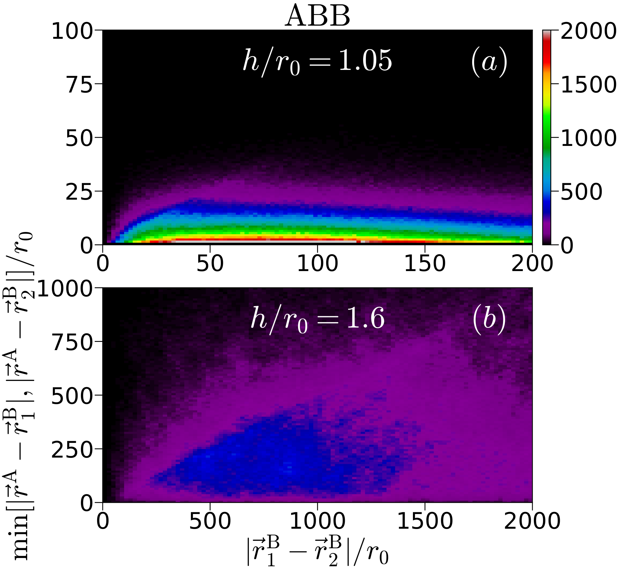
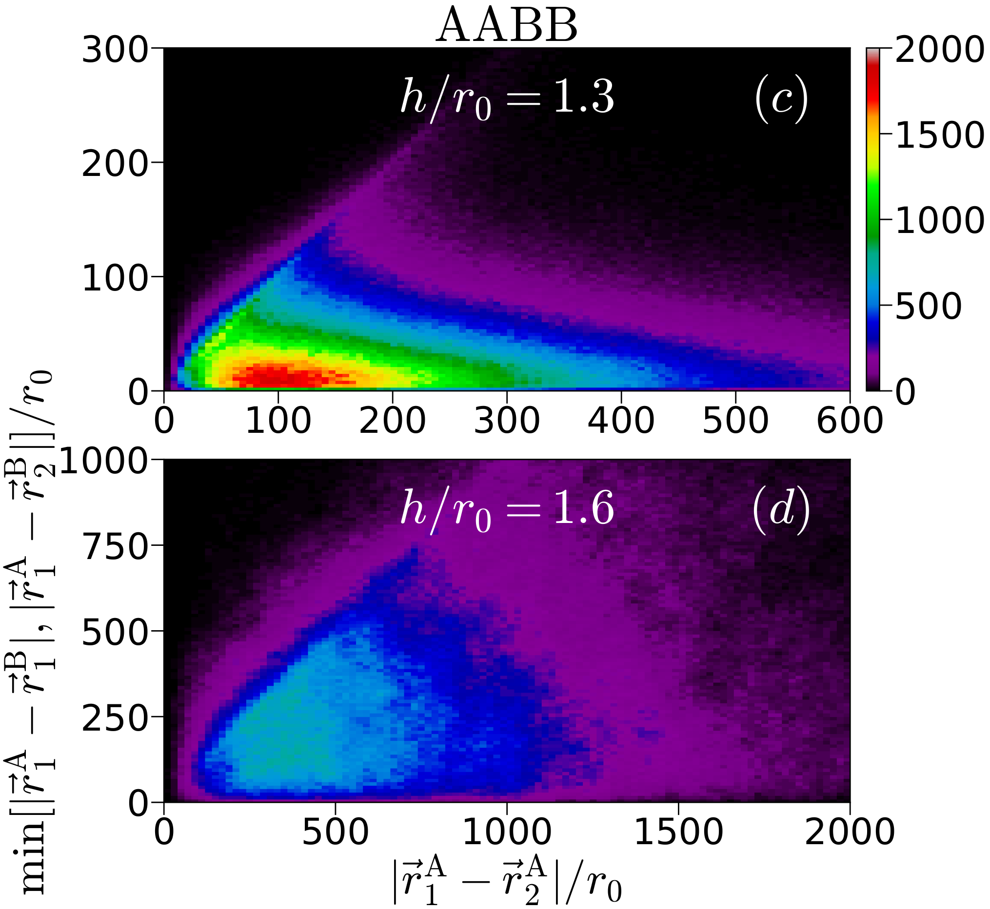
AABB Tetramer
As we have shown in the previous section, an ABB trimer breaks into a dimer and an atom when . Here, we address the structure properties of the balanced case for a tetramer, in which the number of A and B atoms is the same. The AABB tetramer is weakly bound for large values of . When the distance between layers decreases, the tetramer becomes unbound at and splits into two AB dimers [71].
The pair distributions and for AABB are shown in Fig. 5.2 (e, f, g, h) for two characteristic values of the interlayer distance . We observe a behavior that is similar to that previously reported for ABB. That is, both and are compact for the deepest bound state ( for AABB), and become diffuse, showing long tails at large distances when it turns to a weakly-bound state ().
The ground-state spatial distributions for the symmetric tetramer are shown in Fig. 5.3 (c, d). We observe that for large separation , i.e., when the tetramer is weakly bound, it has large spatial extension and the distances between AA and AB pairs are of the same order. As the interlayer separation is progressively decreased, the tetramer size decreases and its structure becomes anisotropic. In this case, the distance between dipoles in the same layer is several times larger than the distance between dipoles in different layers. When the tetramer approaches the threshold for unbinding () the cluster becomes even more elongated and eventually, it breaks into two AB dimers.
5.4.2 Quantum Halo Characteristics
A halo is a quantum bound state in which particles have a high probability to be found in the classically forbidden region, outside the range of the interaction potential. The key characteristic of a halo is its extended size and tiny binding energies. To classify a system as a halo state, one typically introduces two scaling parameters with which the size and the energy are compared. The first parameter is the scaling length . For two-body systems, one commonly chooses as the outer classical turning point. The second parameter is the scaling energy , where is the reduced mass and is the absolute value of the ground-state energy of the cluster. The size of a cluster is usually quantified through its mean-square radius , where is the interparticle distance. A two-body quantum halo is then defined by the condition
| (5.8) |
which means that the system has a probability to be in the classically forbidden region larger than 50.


The dipolar interaction in the bilayer geometry has vanishing Born integral and thus, the AB dimer can show enhanced halo properties. In Fig. 5.4, we show the scaling plot for the dipolar dimers, corresponding to interlayer distance from to 1.6, as indicated on the upper axis. All dimers which lie above the halo limit (horizontal line in Fig. 5.5) are halo states and follow a universal scaling law , shown with a dashed line in the figure [122]. This is exactly the case for all dimers with interlayer separations . This threshold value is close to the characteristic value, , for which the dimer binding energy is approximately equal to the typical energy of the dipolar interaction .


While AB dimers exist for any interlayer separation, ABB trimers and AABB tetramers are self-bound for large values, where AB dimers are in fact halo states. Thus, it can be anticipated that these few-body bound states are also halos. The sizes of three- and four-body systems are measured in terms of the mean-square hyperradius [122],
| (5.9) |
where is an arbitrary mass unit, is the total mass of the system, and is the mass of particle . The scaling size parameter is given by
| (5.10) |
with the two-body scaling length of the system, which is calculated as the outer classical turning point for the potential. We choose equal to zero for repulsive potentials. The condition for three- and four-body quantum halos is now
| (5.11) |
The dependence of the scaled size on the scaled energy for ABB and AABB are shown in Fig. 5.5. We find a non-monotonic behavior, in clear contrast with the dependence observed in the dimer case (see Fig. 5.4). That is, the cluster size decreases with increasing energy and reaches a minimum and then it starts to grow again. The minima correspond to the deepest bound states [71]. This resurgence appears as the clusters approach to the thresholds, where trimers eventually break into a dimer and an atom, and tetramers into two dimers. We want to emphasize that all the trimers and tetramers analized in Fig. 5.5 are halo states, although they are organized in significantly different spatial structures. On the left side of the minima, the clusters are almost radially symmetric and all the interparticle distances are of the same order. However, at the minima and on the right side of the minima, the cluster structures are elongated and highly asymmetric.
The solid line in Fig. 5.5 corresponds to the case of a trimer with contact interactions and without intraspecies repulsion. We observe that the size of the trimer with contact interactions is much smaller than the dipolar trimer, which indicates that repulsion has an important role in the size and energy of the clusters. In the limit of exponentially small energy, large interlayer distance, the dipolar trimer should follow the solid line.
The AABBB pentamer and AAABBB hexamer are self-bound and are manifestly halo states. Their mean square size has a similar behavior to the one observed before for the trimer and tetramer, that is a minimum corresponding to the larger binding energy which separates a regime of nearly symmetric particle distribution form another one, more elongated, and thus asymmetric.
In Fig. 5.6 we plot the cluster size as a function of the binding energy in dipolar units. We notice that the cluster size is a function of the binding energy , as indicated by the black dashed line, and not of the total energy.
Until now, we have shown the size of the clusters as a function of the total and binding energies. Another possibility is to plot the size of the clusters as a function of the interlayer separation , as we can see in Fig. 5.7. Here, for small values of we see a clear separation between population-imbalanced () and population-balanced clusters (). This is a direct consequence of what we found in the previous chapter. That is, in Chapter 4 we find that the few-body bound states in the bilayer geometry have two unbinding thresholds, depending on whether they are balanced or not. The first one is at for population-imbalanced ABB trimer and AABBB pentamer. The second one is at for population-balanced AABB tetramer and AAABBB hexamer.
5.5 Summary
We used the diffusion Monte Carlo method to study the ground-state properties of few-body dipolar bound states in a two-dimensional bilayer setup. We have studied clusters composed by up to six particles, for different values of the interlayer distance, as candidates for quantum halo states. In the case of dimers, we find that for values of the interlayer separation larger than the clusters are halo states and they follow a universal scaling law. In the cases of trimers up to hexamers, we find two very different halo structures. For large values of the interlayer separation, the halo structures are almost radially symmetric and the distances between dipoles are all of the same scales. In contrast, in the vicinity of the threshold for unbinding, the clusters are elongated and highly anisotropic. Importantly, our results prove the existence of stable halo states composed of up to six particles. To the best of our knowledge this is the first time that halo states with such a large number of particles are predicted and observed in a numerical experiment. Indeed, the addition of particles to a two or three body halo states typically makes them shrink towards a more compact liquid structure. This particular bilayer geometry is the reason of our distinct results. We hope that these results will stimulate experimental activity in this setup, composed by atoms with dominant dipolar interaction, to bring evidence of these remarkably quantum halo states.
Chapter 6 Quantum Liquid of Two-Dimensional Dipolar Bosons
In this chapter, we investigate the ground-state phase diagram of two-dimensional dipoles confined to a bilayer geometry by using many-body quantum Monte Carlo methods. The dipoles are considered to be aligned perpendicularly to the parallel layers. We find a rich phase diagram that contains quantum phase transitions between liquid, solid, atomic gas, and molecular gas phases. We predict the formation of a novel liquid phase in which the bosons interact via purely dipolar potential and no contact potential is required to stabilize the system. The liquid phase, which is formed due to the balance between an effective dimer-dimer attraction and an effective three-dimer repulsion, is manifested by the appearance of a minimum in the equation of state. The equilibrium density is given by the position of the minimum of the energy and it can be controlled in a wide range by the interlayer distance. From the equation of state, we extract the spinodal density, below which the homogeneous system experiences a negative pressure and breaks into droplets. Our results offer a new example of a two-dimensional interacting dipolar liquid in a clean and highly controllable setup.
6.1 Introduction
Quantum liquids are self-bound systems, in which competing repulsive and attractive interparticle interactions mechanically balance the system. The effects of quantum mechanics and quantum statistics, such as the indistinguishability of elementary particles, play an important role [141] in the description of these systems. One of the most known quantum liquids is superfluid Helium, which played a revolutionary role in low-temperature quantum physics. The interaction between Helium atoms is characterized by a finite-range potential that has two main features. At large distances, the potential has an attractive long-range van der Waals tail that tends to hold the atoms together. Instead, at short distances, the potential has a strongly repulsive core that prevents the liquid from collapse.
Recent experiments, motivated by a previuos theoretical proposal [5], have enabled the experimental observation of a qualitatively different type of liquid, quantum droplets in a mixture of Bose-Einstein condensates [6, 7, 8] and in dipolar bosonic gases [9, 10, 11, 12]. These quantum droplets are self-bound clusters of atoms possessing a density that is several orders of magnitude more dilute than liquid Helium. Both in two-component and dipolar droplets, the system collapses according to the mean-field theory, thus the stability of the liquid state is a genuinely quantum many-body effect.
Dipolar liquids were first experimentally observed. However, the precise description of the system is complicated because their stability is an interplay between dipolar attraction and short-range repulsion. Therefore, there is a strong dependence on the short-range details of the interaction potential. Instead, dipoles in a bilayer geometry may serve as a simpler and cleaner system in which no short-range repulsion needs to be used. If the dipolar moments of the bosons are oriented perpendicularly to the parallel layers, there is a competing effect between repulsive intralayer and partially attractive interlayer interactions, which can produce interesting few- and many-body states, in particular liquids. For example, a solid and a pair superfluid phases were characterized in Refs. [32, 33] using exact Monte Carlo simulations.
Our results in Chapter 4 for few-body bound states of dipolar bosons confined to a bilayer geometry predicts that a dimer-dimer attraction plus an effective three-dimer repulsion can stabilize a many-body liquid state. It is therefore an open challenge to determine the existence, formation mechanism, and properties of the self-bound many-body system in this geometry.
In this chapter, we study a two-dimensional system of dipolar bosons confined to the bilayer geometry. We calculate the ground-state phase diagram as a function of the density and the separation between layers by using exact quantum Monte Carlo methods. The key result of our work is the prediction of a homogeneous liquid in this system. The liquid is stable in a wide range of densities and interlayer values. We find that the critical interlayer separation at which the liquid to gas transition happens is the same as the threshold value at which the effective interaction between dimers changes from attractive to repulsive and a tetramer is formed in a four-body problem. We characterize the liquid by calculating its equation of state, the condensate fraction, and the equilibrium and spinodal densities.
6.2 The Hamiltonian
We consider bosons of mass and dipole moment confined to two parallel layers separated by a distance . It is assumed that the dipolar moment of each boson is aligned perpendicularly to the planes by the external field. Also, we suppose that the confinement to each plane is so tight that there is no interlayer tunneling and no excitations of the higher levels of the tight confinement are possible. The Hamiltonian of this system is given by
| (6.1) |
where Latin (Greek) indices run over each of () dipoles in the bottom (top) layer. The first two terms in the Hamiltonian (6.1) correspond to the boson kinetic energy, the next two terms are the intralayer dipolar interaction, which is always repulsive and falls off with a power-law . The last term is the interlayer potential which is attractive for small values of but repulsive for large values of , where is the in-plane distance between dipoles. The interlayer potential always supports at least one dimer state. The binding energy diverges for and exponentially vanishes in the opposite limit [88, 89, 90, 91]. The dipolar length is used as a unit of length.
6.3 Details of the Methods
To investigate the ground-state properties of Hamiltonian (6.1) we employ the diffusion Monte Carlo (DMC) method, which was explained in Chapter 2. In this work, we use two guiding trial wave functions, the first one describes two-body correlations between individual dipoles
| (6.2) |
and the second one takes into account a possible formation of AB dimers,
| (6.3) | ||||
Both choices result in a comparable DMC energy, while the convergence is different.
The intraspecies correlations at short distances, , are modeled by the zero-energy two-body scattering solution
| (6.4) |
with the modified Bessel function and a variational parameter [142]. For distances larger than we choose
| (6.5) |
which describes phonons [143]. The constants , and are fixed by imposing continuity of the function and its first derivative at the matching distance , and also that , with the length of the squared simulation box. The interspecies correlations are taken as the solution of the two-body problem up to and imposing the boundary condition . For distances larger than the variational parameter we set . In Fig. 6.1 we show the intraspecies and interspecies wave functions.
For simplicity, we assume a population-balanced system , where is the total number of dipoles. In order to approximate the properties of extended systems, we perform the simulations in a square box with side length and impose periodic boundary conditions. The total density of the system is defined as .
6.4 Results
6.4.1 Finite Size Effects
The dipolar potential is quasi-long ranged in two dimensions, therefore its truncation at produces large finite-size corrections. It is possible to diminish them by adding the contribution of the tail energy to the output of the DMC energy.
For a bilayer system of dipoles the potential energy tail is given by the expression
| (6.6) | ||||
we denote by and the intraspecies and interspecies pair distribution functions, respectively. Substituting the interaction potential expressions
| (6.7) |
in Eq. (6.6) we obtain
| (6.8) |
An approximate value of Eq. (6.8) is obtained by substituting , and , which leads to
| (6.9) |
The total density of the system is , with the total number of particles. The density of each component is one half of the total density, . We now substitute these relations into Eq. (6.9)
| (6.10) |
In units of we get
| (6.11) |
This significantly reduces the finite size dependence on the simulation box length in the energy, while the residual dependence is eliminated by a fitting procedure.
After adding the tail energy to the DMC energy , we extrapolate the energy to the thermodynamic limit value using the fitting formula
| (6.12) |
where C is a fitting parameter.
In Fig. 6.2, we show an example of the finite-size study for the energy. In it, we consider a liquid phase with density and . We observe that the energy dependence on the number of particles scales as , contrary to the law , usual for fast decaying potentials. We find that our fitting function describes well the finite-size dependence. The same procedure is repeated for all the densities for the gas and liquid phases.
6.4.2 Equation of State
A possible existence of a gas or a liquid phase can be determined from the equation of state. The dependence of the energy on density is reported in Fig. 6.3 for different values of the interlayer distance. We have added the contribution of the tail energy Eq. (6.11) and performed the extrapolation to the thermodynamic limit. We observed that for , the energy per particle monotonically increases as the density is increased. Thus, the smallest energy is obtained at vanishing density and this behavior corresponds to a gas phase. However, a drastically different behavior is observed as the interlayer separation is increased. That is, the energy per particle becomes negative and develops a minimum at a finite density for . The position of the minimum corresponds to the equilibrium density. This behavior demonstrates the presence of a homogeneous liquid phase. The balance of forces necessary to stabilize the liquid comes from a dimer-dimer attraction and an effective three-dimer repulsion, as proposed in Chapter 4. Without the repulsive three-dimer force the system would behave as an attractive gas of dimers as shown by the dashed line in Fig. 6.3. We found that the interlayer critical value for the liquid to gas transition () is the same as the threshold value for the four-body bound state of dipolar bosons, when the tetramer breaks into two dimers (Chapter 4).
6.4.3 Phase Diagram
The equations of state are used to extract the equilibrium and spinodal densities, which are defined by the conditions
| (6.13) |
respectively ( being the pressure). The resulting ground-state phase diagram is reported in Fig. 6.4 as a function of the total density and of the interlayer distance . The self-bound many-body phases are formed for large interlayer separation, . Below the spinodal curve (dotted line) the homogeneous liquid is unable to sustain an increasing negative pressure and becomes unstable with respect to droplet formation. The stable liquid phase appears above the spinodal curve. Remarkable, this phase exists in a wide range of densities and interlayer values, which are experimentally accessible. The equilibrium density (dashed line) can be adjusted by changing the separation between the layers: decreases as increases. For large separations , the liquid energy is greatly decreased and in this weakly-interacting regime it is possible to make a comparison with the predictions of Bogoliubov theory [144] for zero-range potential (see Fig. 6.4b). The best agreement is found for the smallest equilibrium and spinodal densities (i.e., for the largest ) for which the dipolar potential is better approximated by the -wave scattering length. The gaseous and self-bound phases are separated by the threshold at which the effective dimer-dimer interaction switches sign [71] (Chapter 4) from repulsion (gas) to attraction (liquid and droplets). The gaseous regime features a second-order phase transition between atomic and molecular gas phases which on a qualitative level occurs when the molecule binding energy is similar to the chemical potential. In the molecular gas phase, the atomic condensate is absent while the molecular one is finite [32]. In the atomic gas, the atomic condensate is present and the system features a strong Andreev-Bahskin drag between superfluids in different layers [34]. The gas phase shows a quantum phase transition from an atomic to a molecular superfluid as the interlayer distance decreases [32].
As the density is increased, the potential energy starts to dominate and a triangular crystal is formed. For large separation between layers, two independent atomic crystals are formed and the phase transition occurs when the density per layer reaches the same critical value as in a single-layer geometry, [142, 145]. In the limit of small interlayer separations, a single molecular crystal is formed at the density .
6.4.4 Depletion of the Condensate
In order to have a more complete description of the liquid and gas phases we have calculated the condensate fraction using the one-body density matrix (OBDM), which is defined as [146]
| (6.14) |
where is the field operator that creates (annihilates) a particle at the point . For a homogeneous system, the condensate fraction is obtained from the asymptotic behavior of the OBDM
| (6.15) |
This behaviour is often referred to as off-diagonal long-range order, since it involves the nondiagonal components of the OBDM. In Fig 6.5 (a) we show an example of the OBDM for different numbers of particles. We notice an important dependence on the total number of particles, that is, the value decreases as the total number of particles increases.
From the VMC and DMC results of the OBDM, we obtained the extrapolated values of , using the extrapolation technique (Section 2.5.3). In Fig 6.5 (b) we plot the extrapolated values of as a function of . In order to remove the finite-size effects, we extrapolate the condensate fraction value to the thermodynamic limit using the fitting formula , where and are fitting parameters.
In Fig. 6.6 (a) we show the condensate fraction as a function of ln, for the dipolar liquid at the equilibrium density. In the dilute limit, we find a good agreement with the quantum depletion calculated in a Bogoliubov theory for short-range potentials. The depletion of the condensate is present in interacting bosonic systems in which, due to the interactions, a portion of bosons are in a non-zero momentum state even at zero temperature. The equilibrium density has a strong dependence on the interlayer separation (see Fig. 6.4). For liquids formed at separations the perturbative result is expected to hold. In the Fig. 6.6 (b) we report the condensate fraction as a function of the interlayer separation . The liquid exists for large separation between the layers . As is decreased the equilibrium density grows up until it reaches at where a phase transition to a gas happens. For smaller separations, the liquid does not exist and we show the condensate fraction in the gas with the density fixed to . The condensate fraction rapidly drops to zero signaling a phase transition from atomic to molecular gas.
6.4.5 Polarization
The different phases present in the system can be further characterized by calculated the ground-state energy dependence on small polarization. This dependence can be linear or quadratic depending on the molecular or atomic nature of the system, respectively. This can be obtained by slightly unbalanced the number of particles in the bottom and top layers, while keeping fixed the total number of particles . The polarization is defined as
| (6.16) |
For an atomic condensate the ground-state energy dependence on small polarization is quadratic
| (6.17) |
where is the ground-state energy of the balanced system and is the spin susceptibility associated with the dispersion of spin waves of the magnetization density with speed of sound . In this case the low-lying excitations are coupled phonon modes of the two layers [32].
For a molecular superfluid phase the ground-state energy is a linear function of the polarization
| (6.18) |
in this case an energy is needed to break a pair and spin excitations are gapped [32].
Examples of the different behaviors of are reported in Fig. 6.7 for three values of corresponding to the molecular gas, atomic gas, and liquid phases. We notice that is a quadratic function of for the liquid state, therefore the liquid is a liquid of atoms and not a liquid of molecules or dimers.
6.5 Summary
We have shown that a dipolar bilayer possesses a rich phase diagram with quantum phase transitions between gas and solid phases (known before), and a liquid phase (newly predicted). Remarkably, the liquid state, which results from the balance of a dimer-dimer attraction and an effective three-dimer repulsion, exists in a wide range of densities and interlayer separations which are experimentally accessible. From the equations of state, we extracted the spinodal and equilibrium densities, which are controllable through the interlayer distance. The equilibrium density decreases as the interlayer distances increases, allowing access to ultra-dilute liquids in a stable setup.
Chapter 7 Phases of Dipolar Bosons Confined to a Multilayer Geometry
7.1 Introduction
In a classical crystal at low temperature all the atoms are strongly localized around their equilibrium lattice positions. In contrast, in a quantum crystal, the atoms move around the equilibrium lattice positions and exchanges between few particles occur with frequency [44]. A quantum crystal is then defined as a crystal in which the zero point motion of an atom about its equilibrium position is a large fraction of the near neighbor distance [147]. This large displacement is a consequence of the light-weight particles and the weakness of the long-range forces between the atoms [44].
The most known quantum solids are Hydrogen and Helium. The solidification of 4He in 1926 initiated the experimental study of quantum solids. 4He solidifies at the temperature limit K under a pressure of bar [147].
An interesting property that quantum solids can exhibit is supersolidity, a state of matter predicted in 1969 for Andreev and Lifshitz in which crystalline order and Bose-Einstein condensation coexists [44]. A supersolid flows without friction but its particles form a crystalline lattice.
Ultracold dipolar gases provide a powerful platform to study highly non-trivial quantum phenomena, in particular to study solid and supersolid states of matter. Recent experimental and theoretical studies have shown that dipolar condensates within a pancake- [77, 148, 149, 150, 151, 152, 153, 154] and cigar-like [155] geometries can undergo a phase transition from a Bose-Einstein condensate (BEC) to a state that has supersolid properties.
An interesting confined system in two dimensions is a layer of dipolar bosons. If the dipolar moments of the bosons are oriented perpendicularly to the layer, the dipole-dipole interaction is repulsive. When this happens, the system undergoes a quantum phase transition from a gas to a solid phase as the density increases [30, 31].
Adding a second parallel layer makes the system richer. In a bilayer setup, there is a competing effect between repulsive intralayer and partially attractive interlayer interactions, which can produce exotic few- and many-body states. For example, a gas and a pair superfluid phases were characterized in Refs. [32, 33] using exact quantum Monte Carlo simulations. Furthermore, when the interlayer distance approaches to zero the system forms a molecular crystal and for large values of the interlayer distance an independent atomic crystal is formed in each layer [145].
In this chapter, we study a system of dipolar bosons confined to a multilayer geometry by using exact many-body quantum Monte Carlo methods. The multilayer geometry consists of equally spaced two-dimensional layers. We consider the case in which the dipoles are aligned perpendicularly to the parallel layers. This system is predicted to have a rich collection of many-body phases due to the anisotropic and quasi long-range dipole-dipole interaction between the bosons. We calculated the ground-state phase diagram as a function of the density, the separation between layers, and the number of layers. The key result of our work is the existence of three phases: atomic gas, solid, and gas of chains, in a wide range of the system parameters. We find that the density of the solid phase decreases several orders of magnitude as the number of layers in the system increases. Furthermore, we calculated the pair distribution functions for the three phases.

7.2 The Hamiltonian
We study an -particle system of dipolar bosons of mass and dipole moment confined to an -layer geometry. The three-dimensional confining structure is formed of two-dimensional parallel layers separated by a distance . The dipolar moment of each boson is considered to be perpendicular to the layers and there is no interlayer tunneling. In Fig. 7.1 we show a schematic representation of the multilayer geometry. The Hamiltonian of this system is given by
| (7.1) |
where is the position vector of particle . The first term in the Hamiltonian (7.1) corresponds to the dipole kinetic energy. The second term is the dipolar interaction between particle and
| (7.2) |
Here, denotes the interlayer separation and stands for the distance between the projections onto any of the layers of the positions of the -th and -th particles. For the dipolar interaction called interlayer interaction, is attractive for small values of but repulsive for large values of , where is the in-plane distance between dipoles. For dipoles in the same layer the dipolar interaction is always repulsive
| (7.3) |
where we set . The dipolar length is used as a unit of length. In Fig. 7.2 we show the dipolar potential as a function of for different values of the interlayer distance , with . Notice that the attractive part of the interlayer potential for and 3 are much weaker than for .
For the Hamiltonian Eq. (7.1) we anticipate to find three phases: atomic gas, solid, and gas of chains. This comes from considering previous studies in a dipolar layer [30, 31] and bilayer [32, 33, 145].
7.3 Details of the Methods
To investigate the ground-state properties of Hamiltonian Eq. (7.1) we employ the diffusion Monte Carlo (DMC) method, which was described in Chapter 2. Here, we use different trial wave functions appropriate for the description of various phases present in the system. In total we describe three phases with different symmetry: gas, solid, and gas of chains.
7.3.1 Gas Trial Wave Function
To describe the gas phase we chose a trial wave function of the Bijl-Jastrow form Eq. (2.75)
| (7.4) |
The wave function has translational symmetry. This symmetry is present in the gas phase, while the crystal phase has broken translational symmetry due to a regular spacing of atoms and, the gas of chains phase has additional interlayer correlations. The two-body terms in Eq. (7.4) depend on the distance between a pair of particles. Here, the two-body terms are taken as the solution of the two-body problem at short distances. This solution depends on whether the dipoles are in the same layer or not. For dipoles in the same layer we chose the short distance part of the two-body correlations term as
| (7.5) |
up to . Here, the modified Bessel function, and are variational parameters [142].
For distances larger than we chose
| (7.6) |
which take into account the contributions from other particles and describe long-range phonons in the form established by Reatto and Chester [143]. The constants , and are fixed by imposing continuity of the function and its first derivative at the matching distance , and also that .
For dipoles in different layers, the interlayer correlations are taken as the solution of the two-body problem up to . We also impose the boundary condition . For distances larger than the variational parameter we set .
7.3.2 Solid Trial Wave Function
The trial wave function we use to describe the quantum solid phase is of the Nosanow-Jastrow form [44]
| (7.7) |
where are the positions vectors of the particles, are the position vectors defining the equilibrium crystal lattice, and and are the one-body and two-body correlation factors, respectively. For a two-dimensional system the equilibrium crystal lattice is a triangular lattice. The wave function (7.7) has a broken translational symmetry due to particle localization close to the lattice sites. In two dimensiones the crystal has triangular symmetry.
The two-body correlation functions used in (7.7) are of the same form as those used to describe the gas phase (7.4), although the specific values of the variational parameters might differ.
The one-body terms used in (7.7) are modeled by a Gaussian function
| (7.8) |
where is the localization strength and is the position of the lattice site. Notice that, are fixed by the triangular lattice. Meanwhile, is a variational parameter, which is chosen by minimizing the variational energy.
The trial wave function (7.7) is not symmetric under the exchange of particles. Therefore, it does not give an appropriate description of off-diagonal properties that directly depend on the Bose-Einstein statistics (for example, one body density matrix and momentum distribution). However, leads to an accurate description of the energy and diagonal properties of quantum solids (for example, density profile, pair-distribution function, static structure factor). Examples of symmetric trial wave functions for modeling quantum solids can be found in Ref. [44]. In this work, we are interested in calculating the ground-state energy and the pair distributions of the system. Thus we will use (7.7). We leave for future work the use of symmetric trial wave functions to describe the properties of our system.
7.3.3 Gas of Chains Trial Wave Function
To describe the gas of chains phase we propose the following trial wave function
| (7.9) |
Differently from the Nosanow-Jastrow wave function, the last product in Eq. (7.9) is not a one-body but rather is a many-body term. That is, the movement of a single particle in that product changes terms, with the number of layers, while in Nosanow form Eq. (7.7) such a movement affects only a single term (i.e. is a one-body correlation). Here, the two-body term depends on the distance between a pair of particles. The many-body term depends on the positions of a single particle and on the center of mass of the chains . Details of the construction of the trial wave function and its derivatives can be found in Section 7.4.
The chain center of mass is given by
| (7.10) |
Here, means that the sum is over all -th particles that belong to the same chain as the -th particle. The main difference with the solid case is that in (7.9) the values change during the simulation while the values in (7.7) are fixed by the triangular lattice.
The two-body correlation functions used in (7.9) are the same as those for the gas and solid phases.
The terms are described by a Gaussian function
| (7.11) |
where is the localization strength.
All the variational parameters that appear in the trial wave functions , and , are chosen by minimizing the variational energy and can have a different value for each trial function.
7.4 Details of the Gas of Chains Wave Function
In this section, we are going to discuss a trial wave function which we employ for the description of a gas of chains phase. Also, we will give explicit expressions for the gradient and Laplacian of the trial function.
While the trial Bijl-Jastrow (gas) and Nosanow-Jastrow (crystal) forms are standard and were extensively studied in the literature, within our best knowledge this is the first time the gas of chains is calculated within the DMC method. For methodological reasons we provide a very detailed description of how such functions are constructed and give explicit expressions of how the derivatives are calculated.
It is essential that the trial wave function has the same symmetry as the one present in the phase. In the gas of chains phase, dipoles belonging to different layers form composite bosons (chains) with no crystal ordering between them. Each composite bosons is composed from dipoles each belonging to a different layer. Also, this gas fulfills the following properties:
- •
The chains are considered to be a composite objects and no exchange of dipoles between them is allowed.
- •
The chains are flexible, each dipole in the chain can move freely in the corresponding layer.
- •
The chains will not become tangled because of the repulsive intralayer interaction between dipoles.
7.4.1 Construction of Trial Wave Function
A trial wave function to describe the gas of chains phase can be constructed as a product of many-body and two-body terms as given in Eq. (7.9). The two-body term depends on the distance between a pair of particles. The many-body term depends on the positions of a single particle and on the the chain center of mass . The chain center of mass itself depends on the positions of particles.
The chain center of mass is given by
| (7.12) |
Here, is the number of layers, and the index runs over all -th particles that belong to the same chain as the -th particle.
In order to implement the QMC algorithm we need to be able to calculate the gradient and Laplacian of the trial wave function. The expressions for the gradient and Laplacian of the two-body terms can be found in the Appendix A. Here, we are going to obtain the expressions for the many-body terms . The gradient of the product of many-body terms with respect to the coordinate is given by
| (7.13) |
Here, is called the center of mass drift force and corresponds to the logarithmic derivative with respect to .
The Laplacian applied with respect to the coordinate reads as
| (7.14) | ||||
Now we can write an expression for the center of mass contribution to the kinetic energy
| (7.15) |
where we have used Eq. (7.13) and we have defined the center of mass local energy as
| (7.16) |
7.4.2 Many-Body Term: Gaussian Function
The purpose of the many-body term in the trial wave function (7.9) is to describe the localization of the particles belonging to one chain around its center of mass. The simplest form of the localization term is a Gaussian function Eq. (7.11)
| (7.17) |
where is the localization strength, is the position vector of the particle and is the chain center of mass to which particle belongs. The chain center of mass is given by Eq. (7.12).
To calculate the center of mass contributions to the drift force (7.13) and local energy (7.16) we need expressions for the gradient and Laplacian of the function (7.17). Let us start by calculating the gradient with respect to the particle
| (7.18) |
where we assumed that .
The Laplacian with respect to the particle reads as
| (7.19) |
where we assumed that .
7.5 Results
In order to approximate the properties of the systems in the thermodynamic limit we perform calculations in finite-size systems with periodic boundary conditions. The total density of the system is defined as , where is the total number of dipoles and is the size of the simulation box. In the gas phase, the simulations are performed in a square box , while in the solid and gas of chains phases the simulations are carried out in a rectangular box , commensurate with the crystal lattice. We ensure that each of the box sides is a multiple of elementary cell size of a triangular lattice.
7.5.1 Crystallization and Threshold Densities
Crystallization Density
In Ref. [31], the authors studied the ground-state phase diagram of a two-dimensional Bose system with dipole-dipole interactions using the QMC methods. The dipoles were constrained to move in a single plane and were polarized in the perpendicular direction to the plane. The authors found a quantum phase transition from a gas to a solid phase as the density increases. This transition was estimated to occur at the critical density
| (7.23) |
with and for a single layer of dipoles.
Our system consists of dipolar bosons confined in an -layer geometry separated by a distance . Now, we are going to show how Eq. (7.23) is rewritten for the system with layers in the limit of rigid chains. To do this, consider a chain with dipoles, one in each layer. When the chain becomes a super-dipole with mass , dipolar moment , and its dipolar length is given by
| (7.24) |
Now consider a -layer system with dipoles and chains evenly distributed. When the -layer system effectively becomes to a single-layer one, each chain becomes a super-dipole, and the number of particles changes from dipoles to super-dipoles. As a consequence of the latter the density now is given by
| (7.25) |
Using Eq. (7.24) and Eq. (7.25) we obtain
| (7.26) |
From the last relation and with Eq. (7.23) we obtain
| (7.27) |
Notably, the solidification density has a strong dependence (fifth power) on the number of layers. In the limit when an -layer system of dipolar bosons will crystallize at the critical density
| (7.28) |
Such a strong dependence on makes the multilayer geometry a very promising setup for future observation of solidification. In Fig. 7.3 we show a schematic representation of the phase diagram of dipolar bosons confined to an -layer geometry. The phase diagram is shown as a function of the total density , the separation between layers , and for different number of layers . The crystallization densities Eq. (7.28) for different values of the number of layers are shown by the thick lines. Notice that the critical density drops several orders of magnitude when going from to 10 layers. This is an important result because it tells us that a very dilute quantum solid can be obtained just by increasing the number of layers in the system.
Threshold Density
The dipolar interlayer potential Eq. (7.2)
| (7.29) |
is anisotropic. It is attractive for small values of but it is repulsive for large values of , where is the in-plane distance between dipoles. Consider an -layer system of dipolar bosons in a solid phase. Here, the system forms a triangular lattice. Now, we ask ourselves what is the threshold distance between a dipole on the first layer and a dipole on the last layer and in a next neighbour lattice site such that the dipolar interlayer potential is zero. This threshold distance can be obtained from Eq. (7.29)
| (7.30) |
with . Now we solve for
| (7.31) |
In Fig. 7.4 we show the interlayer potential as a function of for different values of the number of layers , with . The threshold distances are the points where the potential crosses the horizontal axis. The values of are indicated by arrows in Fig. 7.4.
Now, the mean-inter-particle distance in one layer is proportional to
| (7.32) |
From the Eq. (7.31) and Eq. (7.32) we obtain the threshold density , which satifies Eq. (7.30)
| (7.33) |
The threshold density Eq. (7.33) is an approximation. Densities larger than the threshold density (attractive interlayer potential) will favor the formation of a gas phase and lower densities than the threshold density (repulsive interlayer potential) will favor the formation of the solid phase.
In Fig. 7.3 we plot the threshold density, at which the interaction potential between the most top and most bottom layers changes its sign at the mean interparticle distance, as a function of the interlayer separation and for different values of the number of layers. Each of the shown lines divides the phase diagram into two regions. The first region is above the curve, where the formation of a gas phase is favored. The second region is below the curve where the formation of the solid phase is facilitated. According to the prediction Eq. (7.33), it is possible to have a solid phase at very low densities and for a wide range of .
Finally, we want to emphasize that the equations Eq. (7.28) and Eq. (7.33), which correspond to the crystallization and threshold densities, are approximations under some assumptions. These predictions give us a picture of how the boundaries of the phase diagram are delimited. To calculate the exact phase diagram it is necessary to do DMC calculations, we will do this in the next section.
7.5.2 Dipoles within a Four-Layer Geometry
In this section, we present and discuss our DMC results for the pair distribution functions and the ground-state phase diagram of dipolar bosons confined to a four-layer geometry.
Four-Layer Phase Diagram
The phase diagram of the dipolar multilayer is constructed is the following way. We explore the parameter space (total density and interlayer distance ) and we calculate the ground-state energy with each of the three trial wave functions: , and (see Section 7.3). The phase at each point corresponds to the phase that yields the lowest energy.
The ground-state phase diagram of dipolar bosons within a four-layer geometry is plotted in Fig. 7.5. The phase diagram is shown as a function of the total density and the separation between layers . The crystallization Eq. (7.28) and threshold Eq. (7.33) densities for are shown by the thick and dashed lines, respectively. We found three phases in this system: solid, gas, and gas of chains.
The gas phase and its boundaries were precisely determined, as well as, the transitions solid-gas and chain-gas. However, a precise estimation of the solid-chain transition location is numerally complicated, because the energies of these phases are very similar over a wide range of the parameter space. We expect the gas of chains phase to appear below the crystallization density .
The key result of the phase diagram of Fig. 7.5 is the existence of three phases: gas, solid, and gas of chains, in a wide range of densities and interlayer distances. This characteristic makes the experimental observation of these three phases more feasible.
Pair Distributions
To quantify how the dipoles are spatially distributed in the gas, solid, and gas of chains phases, we calculate the pair distribution function for different values of the system parameters. The pair distribution is proportional to the probability of finding two particles at the relative distance (see Subsection 2.5.1). Here, denotes the interlayer distance between particles. For example, corresponds to the pair distribution of particles in the same layer, corresponds to the pair distribution of particles at a one-layer distance.
In the left panel of Fig. 7.6 we show the pair distribution functions for the gas phase and for . We have set the total density at and interlayer distance . The same-layer distribution vanishes when as a consequence of the strongly repulsive dipolar intralayer potential. As increases, exhibits a shallow maximum, next it tends to 1, the asymptotic value of uncorrelated particles. The strong-correlation peak of at is due to the interlayer attraction. As increases, exhibits a minimum, next it tends to 1. In the left panel of Fig. 7.6 we show a snapshot of the particle coordinates during the DMC simulation. Here, the dipoles are uniformly distributed.
In the left panel of Fig. 7.7 we plot the pair distribution functions for the solid phase and for , with and . When we observe a behavior that is similar to that previously reported for the gas phase. The same-layer distribution start from 0 and the different-layer distributions have a strong correlation peak. As increases the solid pair distributions show a more complex structure than in the case of the gas phase. Here, all show some local maxima and minima rather than tend to 1. These extreme values are related to the parameters of the system, and . The maxima that appear around correspond to the mean interparticle distance and are related to the density of the system. That is, these maxima apper when . In the left panel of Fig. 7.7 we show a snapshot of the particle coordinates during the DMC simulation. Here, the dipoles are distributed in a triangular lattice.
In the left panel of Fig. 7.7 we plot the pair distribution functions for the gas of chains phase and for , with and . When we observe a similar behavior as for the gas and solid phases. As increases shows a maximum, next it tends to 1. The maxima now appear at=20. In the left panel of Fig. 7.8 we show a snapshot of the particle coordinates during the DMC simulation. Here, the dipolar chains are homogeneously distributed.
7.5.3 Dipoles within an M-Layer Geometry
In this section, we present and discuss our DMC results for the phase diagram of dipolar bosons confined to an parallel layers at zero-temperature.
The ground-state phase diagram of dipolar bosons within an -layer geometry is plotted in Fig. 7.9. The phase diagram is shown as a function of the total density , the separation between layers , and for different number of layers . The crystallization and threshold densities are shown by the thick and dashed lines, respectively. The estimated critical interlayer distance for the transition solid-gas is reported for up to 10. For each value of , the critical interlayer distance is reported for one density value.
Notice that, as we increase the number of layers the size of the phase diagram increases for the solid phase. Also that the simple approximation (dashed lines) discussed previously fails dramatically when grows.
7.6 Summary
We used the diffusion Monte Carlo method to study the ground-state phase diagram of dipolar bosons in a geometry formed by equally spaced two-dimensional layers. This system is predicted to have a rich collection of phases due to the anisotropic and quasi long-range dipole-dipole interaction between the bosons. We predicted several quantum phase transitions occurring at zero temperature as the density and separation between layers are changed. First, we have considered the case where there are four layers and the same number of dipoles in each layer. We observe a number of distinct phases, including atomic gas, solid, and gas of chains. These phases are present in a wide range of densities and interlayer distances. The solid phase is predicted to be formed for large densities and small interlayer distances, while the chain phase is presented for lower densities and for a wide range of interlayer distances. The atomic gas is observed in a wide range of densities and interlayers distances. The transitions of solid-gas and chain-gas were determined. Whereas, the exact location of the solid-chain transition could not be determined. Furthermore, we have considered the case where the dipoles are confined up to ten layers. We find that the range of densities where the solid is observed decreases several orders of magnitude with increasing the number of layers in the system. Our results show that the dipolar multilayer system offers a highly controllable setup for observing ultra-dilute quantum solids.
A subject of future work is the implementation of the symmetric trial wave function to describe the solid phase. Also, the calculation of the static structure factor and the superfluid fraction for the solid, gas, and gas of chains. The calculation of these properties will allow us to accurately characterize the solid-chain transition.
Chapter 8 Conclusions
In this Thesis, we reported a detailed study of the ground-state properties of a set of quantum few- and many-body systems. In particular, we have studied one-dimensional Bose-Bose and Fermi-Bose mixtures with attractive interspecies and repulsive intraspecies contact interactions. Here, we characterized a three-dimer repulsion. Also, we have studied a bosonic dipolar quantum system confined to a bilayer and multilayer geometries. These setups consist of equally spaced two-dimensional layers, which can be experimentally realized by imposing tight confinement in one direction. We have studied the bilayer configuration with few and many dipoles and the multilayer system with many dipoles only. In all cases, we used Quantum Monte Carlo simulations to obtain the zero-temperature properties.
Noticeable, we have found in the bilayer that some properties are inherited from the few-dipole system to the many-dipole system. In the case of the few-dipole system, we established the existence of dipolar bound states with interesting properties. For example, we found that the bound states are quantum halo states. In the case of the many-dipole system, we demonstrated the existence of a dilute liquid phase. For the multilayer system we found an extremely dilute solid phase. Our results show that a dipolar system in a bilayer and a multilayer geometries offer clean and highly controllable setups for observing interesting phases of quantum matter, such as, halo states, and dilutes liquids and solids.
Below we present the main conclusions of this Thesis.
One-Dimensional Three-Boson Problem with Two- and Three-Body Interactions
In Chapter 3, by using the diffusion Monte Carlo technique we calculated the binding energy of two and three dimers formed in a one-dimensional Bose-Bose or Fermi-Bose mixture with attractive interspecies and repulsive intraspecies interactions. Combining these results with a three-body theory [57], we extracted the three-dimer scattering length close to the dimer-dimer zero crossing. We argued that since in one dimension the three-body energy correction scales logarithmically with the three-body scattering length , three-body effects are observable even for exponentially small , which significantly simplifies the task of engineering three-body-interacting systems in one dimension. We demonstrated that Bose-Bose or Fermi-Bose dimers, previously shown to be tunable to the dimer-dimer zero crossing, exhibit a noticeable three-dimer repulsion. We can now be certain that the ground state of many such dimers slightly below the dimer-dimer zero crossing is a liquid in which the two-body attraction is compensated by the three-body repulsion [62, 61].
Few-Body Bound States of Two-Dimensional Bosons
In Chapter 4, we have studied few-body clusters of the type ANBM with in a two-dimensional Bose-Bose mixture of A and B bosons, with attractive AB and equally repulsive AA and BB interactions. We considered two very different models: dipolar bosons in a bilayer geometry and particles interacting via separable Gaussian potentials. In both cases, the intraspecies scattering length is of the order of the potential ranges, whereas we tune by adjusting the AB attractive potential (or the interlayer distance in the bilayer setup). We find that for all considered clusters are (weakly) bound and their energies are independent of the interaction model. As the ratio decreases, the increasing intraspecies repulsion pushes the clusters upwards in energy and eventually breaks them up into dimers and free B atoms. In the population balanced case () this happens at where the dimer-dimer attraction changes to repulsion. The population-imbalanced ABB trimer, ABBB tetramer, and AABBB pentamer remain bound beyond the dimer-dimer threshold. In the dipolar model, they break up at where the atom-dimer interaction switches to repulsion. By studying the AAABBB hexamer near the dimer-dimer zero crossing we find that it very much behaves like a system of three point-like particles (dimers) characterized by an effective three-dimer repulsion. A dipolar system in a bilayer geometry can thus exhibit the tunability and mechanical stability necessary for observing dilute liquids and supersolid phases.
Quantum Halo States in Two-Dimensional Dipolar Clusters
In Chapter 5, we have studied the ground-state properties of loosely bound few-body bound states in a two-dimensional bilayer geometry. We have investigated whether halos, bound states with a wave function that extends deeply into the classically forbidden region, can occur in this system. The dipoles are confined to two layers, A and B, with dipolar moments aligned perpendicularly to the layers. We have studied clusters composed by up to six particles, for different values of the interlayer distance, as candidates for quantum halo states. In the case of dimers, we find that for values of the interlayer separation larger than the clusters are halo states and they follow a universal scaling law. In the cases of trimers up to hexamers, we find two very different halo structures. For large values of the interlayer separation, the halo structures are almost radially symmetric and the distances between dipoles are all of the same scales. In contrast, in the vicinity of the threshold for unbinding, the clusters are elongated and highly anisotropic. Importantly, our results prove the existence of stable halo states composed of up to six particles. To the best of our knowledge this is the first time that halo states with such a large number of particles are predicted and observed in a numerical experiment. Indeed, the addition of particles to a two or three body halo states typically makes them shrink towards a more compact liquid structure. This particular bilayer geometry is the reason of our distinct results.
Quantum Liquid of Two-Dimensional Dipolar Bosons
In Chapter 6, we have shown that a dipolar bilayer possesses a rich phase diagram with quantum phase transitions between gas and solid phases (known before), and a liquid phase (newly predicted). Remarkably, the liquid state, which results from the balance of a dimer-dimer attraction and an effective three-dimer repulsion, exists in a wide range of densities and interlayer separations which are experimentally accessible. From the equations of state, we extracted the spinodal and equilibrium densities, which are controllable through the interlayer distance. The equilibrium density decreases as the interlayer distances increases, allowing access to ultra-dilute liquids in a stable setup.
Phases of Dipolar Bosons Confined to a Multilayer Geometry
In Chapter 7, we have studied the ground-state phase diagram of dipolar bosons in a multilayer geometry formed by equally spaced two-dimensional layers. We predicted several quantum phase transitions occurring at zero temperature as the density and separation between layers are changed. We have considered the case where there are four layers and the same number of dipoles in each layer. When the dipole moment of the bosons is aligned perpendicular to the layers, we observe three distinct phases, namely atomic gas, solid, and gas of chains. These phases are present in wide range of densities and interlayer distances. The solid phase is observed for large densities and small interlayer distances. While the chain phase is presented for lower densities and for a wide range of interlayer distances. The atomic gas is observed in a wide range of densities and interlayers distances. The transitions of solid-gas and chains-gas were precisely determined. However, the transition solid-chains could not be fully determined. Furthermore, we have considered the case where the dipoles are confined to three up to ten layers. We find that the range of densities where the solid is observed decreases several orders of magnitude with increasing the number of layers in the system. Our results show that the dipolar multilayer system offers a highly controllable setup for observing ultra-dilute quantum solids.
Chapter A Trial Wave Function
One of the most used many-body trial wave functions in QMC methods for importance sampling is of the form
| (A.1) |
The one-body term depends only on the position of a single particle . The product of two-body terms is known as the Bijl-Jastrow factor. The factor defines the symmetry or antisymmetry of the trial wave function under the exchange of two particles.
In order to implement the QMC algorithm we need to calculate the gradient and Laplacian of the trial wave function. Let us start by obtaining expressions for the gradients involved in Eq. (A.1). The gradient of the product of one-body terms with respect to the coordinate is given by
| (A.2) |
and the gradient of the product of two-body terms is given by
| (A.3) |
Using the expressions shown in the Eq. (A.2) and Eq. (A.3) we obtain an expression for the gradient of the trial wave function with respect to the coordinate
| (A.4) |
Here, is called the drift force. Now we are going to calculate the Laplacian expressions. The Laplacian of the many-body trial wave function with respect to the coordinate is given by
| (A.5) | ||||
where we have used the expresiones Eq. (A.2) and Eq. (A.3). The inner products that appear in Eq. (A.5) are difficult to implement in the QMC code. In order to remove these terms we considered the square of the drift force, from Eq. (A.4) we obtain
| (A.6) | ||||
Now, we solve for the inner product terms
| (A.7) | ||||
After substituting Eq. (A.7) into Eq. (A.5) we get an expression for the Laplacian of the trial wave function with respect to the coordinate and without inner product terms
| (A.8) | ||||
Now we need to calculate the expressions of the Laplacians and and then substitute them in the last equation. The Laplacian is given by
| (A.9) |
and the Laplacian reads as
| (A.10) | ||||
Substituting the Eq. (A.9) and Eq. (A.10) into Eq. (A.8) we obtain an expression for the Laplacian of the trial wave function with respect to the coordinate
| (A.11) | ||||
The Eq. (A.4) and Eq. (A.11) are the equations that are implemented in the QMC code. Now we can write an expression for the kinetic energy
| (A.12) |
where we have used Eq. (A.6) and defined
| (A.13) |
| (A.14) |
| (A.15) |
Chapter B Symmetric Trial Wave Function
An important part of the VMC and DMC methods is the choice of the trial wave function, which is used for importance sampling. Here, we consider a symmetric many-body trial wave function , which is given by
| (B.1) | ||||
We use to study a mixture of A and B bosons with attractive interspecies AB interactions and equally repulsive intraspecies AA and BB interactions. In Eq. (B.1), and are the number of bosons of the species A and B, respectively. We denote with Latin letters the bosons of the species A and with Greek letters the bosons of the species B.
In order to implement the QMC algorithm we need to calculate the gradient and Laplacian of the trial wave function. In the following we are going to obtain the expressions of and . To simplifying the expressions we defined the following quantities
| (B.2) | |||||
With the above definitions the trial wave function Eq. (B.1) reduces to
| (B.3) |
Let us now obtain expressions for the gradients involved in Eq. (B.1). The gradient of the trial wave function with respect to the coordinate is given by
| (B.4) |
Here, is called the drift force. The term does not appears in Eq. (B.4), because is independent of the coordinate . The expressions of the gradients , and with respect to the coordinate are given by
| (B.5) | ||||
Now we are going to calculate the expressions for the Laplacians involved in Eq. (B.1). The Laplacian of the trial wave function with respect to the coordinate is given by
| (B.6) |
The second term in the right hand side of Eq. (B.6) is difficult to calculate in the DMC code, since it involves the inner product of different quantities. To remove this term let us to calculate the square of the drift force, from Eq. (B.4) we obtain
| (B.7) |
Now we solve for the inner product term
| (B.8) |
After substituting Eq. (B.8) into Eq. (B.6) we obtain a expression for the Laplacian of the trial wave function
| (B.9) | ||||
Here, we see that is given in terms of the gradients and Laplacians of , and . We already derived expressions for the gradients, which are given in Eq. (B.5). Now, we focus on obtaining expressions for , and . The Laplacian reads as
| (B.10) | ||||
The Laplacian is given by the following expression
| (B.11) |
And finally, the Laplacian is given by
| (B.12) | ||||
The full Laplacian of the many-body trial wave function with respect to the coordinate is given by
| (B.13) | ||||
Analogous to the Eq. (B.13), the full Laplacian of the many-body trial wave function with respect to the coordinate is given by
| (B.14) | ||||
Here, the drift force with respect to the coordinate is given by
| (B.15) |
In the following we are going to obtain the expressions for the gradients and Laplacians involved in Eq. (B.14). The gradients , and are given by
| (B.16) | ||||
The Laplacian is given by
| (B.17) | ||||
The expression for the Laplacian reads as
| (B.18) | ||||
Finally, the Laplacian is given by
| (B.19) |
References
- [1] A. Einstein. Quantentheorie des einatomigen idealen gases. Sitzungsberichte der Preussischen Akademie der Wissenschaften, page 261–267, 1924.
- [2] M. H. Anderson, J. R. Ensher, M. R. Matthews, C. E. Wieman, and E. A. Cornell. Observation of Bose-Einstein condensation in a dilute atomic vapor. Science, 269(5221):198–201, 1995.
- [3] K. B. Davis, M. O. Mewes, M. R. Andrews, N. J. van Druten, D. S. Durfee, D. M. Kurn, and W. Ketterle. Bose-Einstein condensation in a gas of sodium atoms. Phys. Rev. Lett., 75:3969–3973, Nov 1995.
- [4] www.nobelprize.org.
- [5] D. S. Petrov. Quantum mechanical stabilization of a collapsing Bose-Bose mixture. Phys. Rev. Lett., 115:155302, Oct 2015.
- [6] C. R. Cabrera, L. Tanzi, J. Sanz, B. Naylor, P. Thomas, P. Cheiney, and L. Tarruell. Quantum liquid droplets in a mixture of Bose-Einstein condensates. Science, 359(6373):301, 2018.
- [7] G. Semeghini, G. Ferioli, L. Masi, C. Mazzinghi, L. Wolswijk, F. Minardi, M. Modugno, G. Modugno, M. Inguscio, and M. Fattori. Self-bound quantum droplets of atomic mixtures in free space. Phys. Rev. Lett., 120:235301, Jun 2018.
- [8] G. Ferioli, G. Semeghini, L. Masi, G. Giusti, G. Modugno, M. Inguscio, A. Gallemí, A. Recati, and M. Fattori. Collisions of self-bound quantum droplets. Phys. Rev. Lett., 122:090401, Mar 2019.
- [9] H. Kadau, M Schmitt, M. Wenzel, C Wink, T. Maier, I. Ferrier-Barbut, and T. Pfau. Observing the Rosensweig instability of a quantum ferrofluid. Nature, 530(7589):194, February 2016.
- [10] M. Schmitt, M. Wenzel, F. Böttcher, I. Ferrier-Barbut, and T. Pfau. Self-bound droplets of a dilute magnetic quantum liquid. Nature (London), 539:259, 2016.
- [11] I. Ferrier-Barbut, H. Kadau, M. Schmitt, M. Wenzel, and T. Pfau. Observation of quantum droplets in a strongly dipolar Bose gas. Phys. Rev. Lett., 116:215301, 2016.
- [12] L. Chomaz, S. Baier, D. Petter, M. J. Mark, F. Wächtler, L. Santos, and F. Ferlaino. Quantum-fluctuation-driven crossover from a dilute Bose-Einstein condensate to a macrodroplet in a dipolar quantum fluid. Phys. Rev. X, 6:041039, 2016.
- [13] Ivan Morera, Grigori E. Astrakharchik, Artur Polls, and Bruno Juliá-Díaz. Quantum droplets of bosonic mixtures in a one-dimensional optical lattice. Phys. Rev. Research, 2:022008, Apr 2020.
- [14] Ivan Morera, Grigori E. Astrakharchik, Artur Polls, and Bruno Juliá-Díaz. Universal dimerized quantum droplets in a one-dimensional lattice, arXiv 2007.01786 2020.
- [15] Christoph Kohstall, Mattheo Zaccanti, Matthias Jag, Andreas Trenkwalder, Pietro Massignan, Georg M Bruun, Florian Schreck, and Rudolf Grimm. Metastability and coherence of repulsive polarons in a strongly interacting Fermi mixture. Nature, 485(7400):615–618, 2012.
- [16] Pietro Massignan, Matteo Zaccanti, and Georg M Bruun. Polarons, dressed molecules and itinerant ferromagnetism in ultracold Fermi gases. Reports on Progress in Physics, 77(3):034401, feb 2014.
- [17] Raúl Bombín, Tommaso Comparin, Gianluca Bertaina, Ferran Mazzanti, Stefano Giorgini, and Jordi Boronat. Two-dimensional repulsive Fermi polarons with short and long-range interactions. Phys. Rev. A, 100:023608, 2019.
- [18] Shuhei M. Yoshida, Shimpei Endo, Jesper Levinsen, and Meera M. Parish. Universality of an impurity in a Bose-Einstein condensate. Phys. Rev. X, 8:011024, Feb 2018.
- [19] Nils-Eric Guenther, Pietro Massignan, Maciej Lewenstein, and Georg M. Bruun. Bose polarons at finite temperature and strong coupling. Phys. Rev. Lett., 120:050405, Feb 2018.
- [20] L. A. Peña Ardila, G. E. Astrakharchik, and S. Giorgini. Strong coupling Bose polarons in a two-dimensional gas. Phys. Rev. Research, 2:023405, Jun 2020.
- [21] T Lahaye, C Menotti, L Santos, M Lewenstein, and T Pfau. The physics of dipolar bosonic quantum gases. Reports on Progress in Physics, 72(12):126401, nov 2009.
- [22] Axel Griesmaier, Jörg Werner, Sven Hensler, Jürgen Stuhler, and Tilman Pfau. Bose-Einstein condensation of chromium. Phys. Rev. Lett., 94:160401, Apr 2005.
- [23] J. Stuhler, A. Griesmaier, T. Koch, M. Fattori, T. Pfau, S. Giovanazzi, P. Pedri, and L. Santos. Observation of dipole-dipole interaction in a degenerate quantum gas. Phys. Rev. Lett., 95:150406, Oct 2005.
- [24] Mingwu Lu, Nathaniel Q. Burdick, Seo Ho Youn, and Benjamin L. Lev. Strongly dipolar Bose-Einstein condensate of dysprosium. Phys. Rev. Lett., 107:190401, Oct 2011.
- [25] Mingwu Lu, Nathaniel Q. Burdick, and Benjamin L. Lev. Quantum degenerate dipolar Fermi Gas. Phys. Rev. Lett., 108:215301, May 2012.
- [26] Lauriane Chomaz, Rick Bijnen, Daniel Petter, Giulia Faraoni, Simon Baier, Jan Becher, Falk Waechtler, Luis Santos, and Francesca Ferlaino. Observation of the roton mode in a dipolar quantum gas. Nature Physics, 14, 05 2018.
- [27] R. Bombin, J. Boronat, and F. Mazzanti. Dipolar Bose supersolid stripes. Phys. Rev. Lett., 119:250402, Dec 2017.
- [28] A. Trautmann, P. Ilzhöfer, G. Durastante, C. Politi, M. Sohmen, M. J. Mark, and F. Ferlaino. Dipolar quantum mixtures of erbium and dysprosium atoms. Phys. Rev. Lett., 121:213601, Nov 2018.
- [29] Tommaso Comparin, Raúl Bombín, Markus Holzmann, Ferran Mazzanti, Jordi Boronat, and Stefano Giorgini. Two-dimensional mixture of dipolar fermions: Equation of state and magnetic phases. Phys. Rev. A, 99:043609, Apr 2019.
- [30] H.-P. Büchler, E. Demler, M. Lukin, A. Micheli, N. Prokof’ev, G. Pupillo, and P. Zoller. Strongly correlated 2D quantum phases with cold polar molecules: Controlling the shape of the interaction potential. Phys. Rev. Lett., 98:060404, Feb 2007.
- [31] G. E. Astrakharchik, J. Boronat, I. L. Kurbakov, and Yu. E. Lozovik. Quantum phase transition in a two-dimensional system of dipoles. Phys. Rev. Lett., 98:060405, Feb 2007.
- [32] A. Macia, G. E. Astrakharchik, F. Mazzanti, S. Giorgini, and J. Boronat. Single-particle versus pair superfluidity in a bilayer system of dipolar bosons. Phys. Rev. A, 90:043623, Oct 2014.
- [33] G. E. Astrakharchik, R. E. Zillich, F. Mazzanti, and J. Boronat. Gapped spectrum in pair-superfluid bosons. Phys. Rev. A, 94:063630, Dec 2016.
- [34] J. Nespolo, G. E. Astrakharchik, and A. Recati. Andreev–Bashkin effect in superfluid cold gases mixtures. New J. Phys., 19(12):125005, dec 2017.
- [35] B.L. Hammond, W.A. Lester, and P.J. Reynolds. Monte Carlo Methods in Ab Initio Quantum Chemistry. Lecture and Course Notes In Chemistry Series. World Scientific, 1994.
- [36] Julien Toulouse, Roland Assaraf, and C. J. Umrigar. Introduction to the variational and diffusion Monte Carlo methods, 2015.
- [37] David Ceperley. An Overview of Quantum Monte Carlo Methods. Reviews in Mineralogy & Geochemistry - REV MINERAL GEOCHEM, 71:129–135, 04 2010.
- [38] V. Cikojević, L. Vranje š Markić, G. E. Astrakharchik, and J. Boronat. Universality in ultradilute liquid bose-bose mixtures. Phys. Rev. A, 99:023618, Feb 2019.
- [39] L. Parisi, G. E. Astrakharchik, and S. Giorgini. The liquid state of one-dimensional Bose mixtures: a quantum Monte-Carlo study. Phys. Rev. Lett., 122:105302, 2019.
- [40] L. A. Peña Ardila, N. B. Jørgensen, T. Pohl, S. Giorgini, G. M. Bruun, and J. J. Arlt. Analyzing a Bose polaron across resonant interactions. Phys. Rev. A, 99:063607, Jun 2019.
- [41] O. A. Rodríguez López. Interacting Bose gas in multi-rod lattices : ground state properties and quantum phase transitions. PhD thesis, UNAM, Instituto de Física, 2020.
- [42] J. Sánchez-Baena, J. Boronat, and F. Mazzanti. Diffusion Monte Carlo methods for spin-orbit-coupled ultracold Bose gases. Phys. Rev. A, 98:053632, Nov 2018.
- [43] Matthew Foulkes, L. Mitas, R. Needs, and Guna Rajagopal. Quantum Monte Carlo simulation of solids. Reviews of Modern Physics, 73, 02 2001.
- [44] Claudio Cazorla and Jordi Boronat. Simulation and understanding of atomic and molecular quantum crystals. Rev. Mod. Phys., 89:035003, Aug 2017.
- [45] W. Dmowski, S. O. Diallo, K. Lokshin, G. Ehlers, G. Ferré, J. Boronat, and T. Egami. Observation of dynamic atom-atom correlation in liquid Helium in real space. Nature Communications, 8:15294, 2017.
- [46] M. C. Gordillo and J. Boronat. Superfluid and supersolid phases of on the second layer of graphite. Phys. Rev. Lett., 124:205301, May 2020.
- [47] W. L. McMillan. Ground state of liquid He4. Phys. Rev., 138:A442–A451, Apr 1965.
- [48] Rafael Guardiola. Monte Carlo methods in quantum many-body theories. In Jesús Navarro and Artur Polls, editors, Microscopic Quantum Many-Body Theories and Their Applications, pages 269–336, Berlin, Heidelberg, 1998. Springer Berlin Heidelberg.
- [49] Peter J. Reynolds, David M. Ceperley, Berni J. Alder, and William A. Lester. Fixed‐node quantum Monte Carlo for molecules. The Journal of Chemical Physics, 77(11):5593–5603, 1982.
- [50] G. Ferré Porta. A Monte Carlo approach to statics and dynamics of quantum fluids. PhD thesis, UPC, Departament de Física Aplicada, 2017.
- [51] R. Bombín Escudero. Ultracold Bose and Fermi dipolar gases: a Quantum Monte Carlo study. PhD thesis, UPC, Departament de Física Aplicada, 2019.
- [52] Ioan Kosztin, Byron Faber, and Klaus Schulten. Introduction to the diffusion Monte Carlo method. American Journal of Physics, 64(5):633–644, 1996.
- [53] Siu A. Chin. Quadratic diffusion Monte Carlo algorithms for solving atomic many-body problems. Phys. Rev. A, 42:6991–7005, Dec 1990.
- [54] K. S. Liu, M. H. Kalos, and G. V. Chester. Quantum hard spheres in a channel. Phys. Rev. A, 10:303–308, Jul 1974.
- [55] J. Casulleras and J. Boronat. Unbiased estimators in quantum Monte Carlo methods: Application to liquid . Phys. Rev. B, 52:3654–3661, Aug 1995.
- [56] A. Sarsa, J. Boronat, and J. Casulleras. Quadratic diffusion Monte Carlo and pure estimators for atoms. The Journal of Chemical Physics, 116(14):5956–5962, 2002.
- [57] G. Guijarro, A. Pricoupenko, G. E. Astrakharchik, J. Boronat, and D. S. Petrov. One-dimensional three-boson problem with two- and three-body interactions. Phys. Rev. A, 97:061605, Jun 2018.
- [58] Elliott H. Lieb and Werner Liniger. Exact analysis of an interacting Bose gas. I. The general solution and the ground state. Phys. Rev., 130:1605–1616, May 1963.
- [59] J. B. McGuire. Study of exactly soluble one‐dimensional N‐body problems. Journal of Mathematical Physics, 5(5):622–636, 1964.
- [60] Yuta Sekino and Yusuke Nishida. Quantum droplet of one-dimensional bosons with a three-body attraction. Phys. Rev. A, 97:011602, Jan 2018.
- [61] A. Pricoupenko and D. S. Petrov. Dimer-dimer zero crossing and dilute dimerized liquid in a one-dimensional mixture. Phys. Rev. A, 97:063616, Jun 2018.
- [62] Aurel Bulgac. Dilute quantum droplets. Phys. Rev. Lett., 89:050402, Jul 2002.
- [63] D. S. Petrov. Three-body interacting bosons in free space. Phys. Rev. Lett., 112:103201, Mar 2014.
- [64] M. Girardeau. Relationship between systems of impenetrable bosons and fermions in one dimension. Journal of Mathematical Physics, 1(6):516–523, 1960.
- [65] Stephan Falke, Horst Knöckel, Jan Friebe, Matthias Riedmann, Eberhard Tiemann, and Christian Lisdat. Potassium ground-state scattering parameters and Born-Oppenheimer potentials from molecular spectroscopy. Phys. Rev. A, 78:012503, Jul 2008.
- [66] Cheng-Hsun Wu, Ibon Santiago, Jee Woo Park, Peyman Ahmadi, and Martin W. Zwierlein. Strongly interacting isotopic Bose-Fermi mixture immersed in a Fermi sea. Phys. Rev. A, 84:011601, Jul 2011.
- [67] M. Olshanii. Atomic scattering in the presence of an external confinement and a gas of impenetrable bosons. Phys. Rev. Lett., 81:938–941, Aug 1998.
- [68] A. Muryshev, G. V. Shlyapnikov, W. Ertmer, K. Sengstock, and M. Lewenstein. Dynamics of dark solitons in elongated Bose-Einstein condensates. Phys. Rev. Lett., 89:110401, Aug 2002.
- [69] Subhasis Sinha, Alexander Yu. Cherny, Dmitry Kovrizhin, and Joachim Brand. Friction and diffusion of matter-wave bright solitons. Phys. Rev. Lett., 96:030406, Jan 2006.
- [70] I. E. Mazets, T. Schumm, and J. Schmiedmayer. Breakdown of integrability in a quasi-1d ultracold bosonic gas. Phys. Rev. Lett., 100:210403, May 2008.
- [71] G. Guijarro, G. E. Astrakharchik, J. Boronat, B. Bazak, and D. S. Petrov. Few-body bound states of two-dimensional bosons. Phys. Rev. A, 101:041602, Apr 2020.
- [72] A. Pricoupenko and D. S. Petrov. Dimer-dimer zero crossing and dilute dimerized liquid in a one-dimensional mixture. Phys. Rev. A, 97:063616, 2018.
- [73] D.-W. Wang, M. D. Lukin, and E. Demler. Quantum fluids of self-assembled chains of polar molecules. Phys. Rev. Lett., 97:180413, Nov 2006.
- [74] D.-W. Wang. Quantum phase transitions of polar molecules in bilayer systems. Phys. Rev. Lett., 98:060403, Feb 2007.
- [75] Trefzger C., Menotti C., Capogrosso-Sansone B., and Lewenstein M. Ultracold dipolar gases in optical lattices. Journal of Physics B: Atomic, Molecular and Optical Physics, 44(19):193001, sep 2011.
- [76] D. H. J. O’Dell, S. Giovanazzi, and G. Kurizki. Rotons in gaseous Bose-Einstein condensates irradiated by a laser. Phys. Rev. Lett., 90:110402, Mar 2003.
- [77] L. Santos, G. V. Shlyapnikov, and M. Lewenstein. Roton-Maxon spectrum and stability of trapped dipolar Bose-Einstein condensates. Phys. Rev. Lett., 90:250403, Jun 2003.
- [78] Z.-K. Lu, Y. Li, D. S. Petrov, and G. V. Shlyapnikov. Stable dilute supersolid of two-dimensional dipolar bosons. Phys. Rev. Lett., 115:075303, 2015.
- [79] L. Tanzi, E. Lucioni, F. Famà, J. Catani, A. Fioretti, C. Gabbanini, R. N. Bisset, L. Santos, and G. Modugno. Observation of a dipolar quantum gas with metastable supersolid properties. Phys. Rev. Lett., 122:130405, Apr 2019.
- [80] L. Chomaz, D. Petter, P. Ilzhöfer, G. Natale, A. Trautmann, C. Politi, G. Durastante, R. M. W. van Bijnen, A. Patscheider, M. Sohmen, M. J. Mark, and F. Ferlaino. Long-lived and transient supersolid behaviors in dipolar quantum gases. Phys. Rev. X, 9:021012, 2019.
- [81] F. Böttcher, J.-N. Schmidt, M. Wenzel, J. Hertkorn, M. Guo, T. Langen, and T. Pfau. Transient supersolid properties in an array of dipolar quantum droplets. Phys. Rev. X, 9:011051, 2019.
- [82] L. Tanzi, S. M. Roccuzzo, E. Lucioni, F. Famà, A. Fioretti, C. Gabbanini, G. Modugno, A. Recati, and S. Stringari. Supersolid symmetry breaking from compressional oscillations in a dipolar quantum gas. Nature (London), 574:382, 2019.
- [83] M. Guo, F. Böttcher, J. Hertkorn, J.-N. Schmidt, M. Wenzel, H.-P. Büchler, T. Langen, and T. Pfau. The low-energy goldstone mode in a trapped dipolar supersolid. Nature (London), 574:386, 2019.
- [84] G. Natale, R. M. W. van Bijnen, A. Patscheider, D. Petter, M. J. Mark, L. Chomaz, and F. Ferlaino. Excitation spectrum of a trapped dipolar supersolid and its experimental evidence. Phys. Rev. Lett., 123:050402, Aug 2019.
- [85] A. Safavi-Naini, Ş. G. Söyler, G. Pupillo, H. R. Sadeghpour, and B. Capogrosso-Sansone. Quantum phases of dipolar bosons in bilayer geometry. New J. Phys., 15:013036, 2013.
- [86] Note that the analogous integral in the bitube geometry is finite [see, for example, B. Wunsch, N. T. Zinner, I. B. Mekhov, S.-J. Huang, D.-W. Wang, and E. Demler, Few-Body Bound States in Dipolar Gases and Their Detection, Phys. Rev. Lett. 107, 073201 (2011)].
- [87] V. I. Yudson, M. G. Rozman, and P. Reineker. Bound states of two particles confined to parallel two-dimensional layers and interacting via dipole-dipole or dipole-charge laws. Phys. Rev. B, 55:5214, Feb 1997.
- [88] S.-M. Shih and D.-W. Wang. Pseudopotential of an interaction with a power-law decay in two-dimensional systems. Phys. Rev. A, 79:065603, 2009.
- [89] J. R. Armstrong, N. T. Zinner, D. V. Fedorov, and A. S. Jensen. Bound states and universality in layers of cold polar molecules. Europhys. Lett., 91:16001, 2010.
- [90] M. Klawunn, A. Pikovski, and L. Santos. Two-dimensional scattering and bound states of polar molecules in bilayers. Phys. Rev. A, 82:044701, Oct 2010.
- [91] M. A. Baranov, A. Micheli, S. Ronen, and P. Zoller. Bilayer superfluidity of fermionic polar molecules: Many-body effects. Phys. Rev. A, 83:043602, Apr 2011.
- [92] A. G. Volosniev, D. V. Fedorov, A. S. Jensen, and N. T. Zinner. Model independence in two dimensions and polarized cold dipolar molecules. Phys. Rev. Lett., 106:250401, 2011.
- [93] B. Simon. The bound state of weakly coupled Schrödinger operators in one and two dimensions. Annals of Physics, 97(2):279, April 1976.
- [94] A. G. Volosniev, D. V. Fedorov, A. S. Jensen, and N. T. Zinner. Few-body bound-state stability of dipolar molecules in two dimensions. Phys. Rev. A, 85:023609, Feb 2012.
- [95] C. Ticknor. Two-dimensional dipolar scattering. Phys. Rev. A, 80:052702, 2009.
- [96] Y. Suzuki and K. Varga. Stochastic variational approach to quantum-mechanical few-body problems. Springer, Berlin Heidelberg, 1998.
- [97] B. Bazak, M. Eliyahu, and U. van Kolck. Effective field theory for few-boson systems. Phys. Rev. A, 94:052502, 2016.
- [98] I. V. Brodsky, M. Yu. Kagan, A. V. Klaptsov, R. Combescot, and X. Leyronas. Exact diagrammatic approach for dimer-dimer scattering and bound states of three and four resonantly interacting particles. Phys. Rev. A, 73:032724, 2006.
- [99] L. Pricoupenko and P. Pedri. Universal (1+2)-body bound states in planar atomic waveguides. Phys. Rev. A, 82:033625, 2010.
- [100] F. F. Bellotti, T. Frederico, M. T. Yamashita, D. V. Fedorov, A. S. Jensen, and N. T. Zinner. Scaling and universality in two dimensions: three-body bound states with short-ranged interactions. J. Phys. B: At Mol. Opt. Phys., 44:205302, 2011.
- [101] B. Bazak and D. S. Petrov. Energy of N two-dimensional bosons with zero-range interactions. New J. Phys., 20(2):023045, 2018.
- [102] T. Ren and I. Aleiner. Three-boson bound states in three dimensions. Phys. Rev. B, 95:045401, 2017.
- [103] B. Bazak and D. S. Petrov. Stable -wave resonant two-dimensional Fermi-Bose dimers. Phys. Rev. Lett., 121:263001, 2018.
- [104] M.Y. Kagan. Modern trends in Superconductivity and Superfluidity. Lecture Notes in Physics. Springer Netherlands, 2013.
- [105] M. Inguscio, W. Ketterle, and C. Salomon. Ultra-cold Fermi Gases. International School of Physics “Enrico Fermi”. IOS Press, 2008.
- [106] L. W. Bruch and J. A. Tjon. Binding of three identical bosons in two dimensions. Phys. Rev. A, 19:425, 1979.
- [107] Sadhan K. Adhikari, A. Delfino, T. Frederico, I. D. Goldman, and Lauro Tomio. Efimov and Thomas effects and the model dependence of three-particle observables in two and three dimensions. Phys. Rev. A, 37:3666–3673, May 1988.
- [108] E. Nielsen, D. V. Fedorov, and A. S. Jensen. Three-body halos in two dimensions. Phys. Rev. A, 56:3287, 1997.
- [109] E. Nielsen, D. V. Fedorov, and A. S. Jensen. Structure and occurrence of three-body halos in two dimensions. Few-Body Syst., 27:15, 1999.
- [110] H.-W. Hammer and D. T. Son. Universal properties of two-dimensional boson droplets. Phys. Rev. Lett., 93:250408, Dec 2004.
- [111] O. I. Kartavtsev and A. V. Malykh. Universal low-energy properties of three two-dimensional bosons. Phys. Rev. A, 74:042506, Oct 2006.
- [112] T. Takekoshi, L. Reichsöllner, A. Schindewolf, J. M. Hutson, C. R. Le Sueur, O. Dulieu, F. Ferlaino, R. Grimm, and H.-C. Nägerl. Ultracold dense samples of dipolar RbCs molecules in the rovibrational and hyperfine ground state. Phys. Rev. Lett., 113:205301, Nov 2014.
- [113] P. K. Molony, P. D. Gregory, Z. Ji, B. Lu, M. P. Köppinger, C. R. Le Sueur, C. L. Blackley, J. M. Hutson, and S. L. Cornish. Creation of ultracold molecules in the rovibrational ground state. Phys. Rev. Lett., 113:255301, Dec 2014.
- [114] M. Guo, B. Zhu, B. Lu, X. Ye, F. Wang, R. Vexiau, N. Bouloufa-Maafa, G. Quéméner, O. Dulieu, and D. Wang. Creation of an ultracold gas of ground-state dipolar molecules. Phys. Rev. Lett., 116:205303, May 2016.
- [115] M. Guo, X. Ye, J. He, G. Quéméner, and D. Wang. High-resolution internal state control of ultracold molecules. Phys. Rev. A, 97:020501(R), Feb 2018.
- [116] J. Deiglmayr, A. Grochola, M. Repp, O. Dulieu, R. Wester, and M. Weidemüller. Permanent dipole moment of LiCs in the ground state. Phys. Rev. A, 82:032503, Sep 2010.
- [117] S. A. Moses, J. P. Covey, M. T. Miecnikowski, B. Yan, B. Gadway, J. Ye, and D. S. Jin. Creation of a low-entropy quantum gas of polar molecules in an optical lattice. Science, 350(6261):659, 2015.
- [118] L. De Marco, G. Valtolina, K. Matsuda, W. G. Tobias, J. P. Covey, and J. Ye. A degenerate Fermi gas of polar molecules. Science, 363(6429):853, 2019.
- [119] J. W. Park, S. A. Will, and M. W. Zwierlein. Ultracold dipolar gas of fermionic molecules in their absolute ground state. Phys. Rev. Lett., 114:205302, 2015.
- [120] J. W. Park, Z. Z. Yan, H. Loh, S. A. Will, and M. W. Zwierlein. Second-scale nuclear spin coherence time of ultracold molecules. Science, 357:372, 2017.
- [121] H. Yang, D.-C. Zhang, L. Liu, Y.-X. Liu, J. Nan, B. Zhao, and J.-W. Pan. Observation of magnetically tunable feshbach resonances in ultracold + collisions. Science, 363:261, 2019.
- [122] A. S. Jensen, K. Riisager, D. V. Fedorov, and E. Garrido. Structure and reactions of quantum halos. Rev. Mod. Phys., 76:215–261, Feb 2004.
- [123] K Riisager. Halos and related structures. Physica Scripta, T152:014001, jan 2013.
- [124] V. Efimov. Energy levels arising from resonant two-body forces in a three-body system. Physics Letters B, 33(8):563 – 564, 1970.
- [125] T Kraemer, Manfred Mark, Philipp Waldburger, Johann G Danzl, Cheng Chin, Bastian Engeser, Almar D Lange, Karl Pilch, Antti Jaakkola, H-C Nägerl, et al. Evidence for Efimov quantum states in an ultracold gas of caesium atoms. Nature, 440(7082):315–318, 2006.
- [126] Pascal Naidon and Shimpei Endo. Efimov physics: a review. Reports on Progress in Physics, 80(5):056001, mar 2017.
- [127] Subir Sachdev. Quantum phase transitions. Cambridge Univ. Press, 2009.
- [128] Immanuel Bloch and Immanuel. Ultracold quantum gases in optical lattices. Nat. Phys., 1:23–30, 10 2005.
- [129] Stefano Giorgini, Lev P. Pitaevskii, and Sandro Stringari. Theory of ultracold atomic Fermi gases. Rev. Mod. Phys., 80:1215–1274, Oct 2008.
- [130] Wilhelm Zwerger. The BCS-BEC crossover and the unitary Fermi gas. Springer, Heidelberg New York, 2012.
- [131] K. Riisager. Nuclear halo states. Rev. Mod. Phys., 66:1105–1116, Jul 1994.
- [132] I. Tanihata, H. Hamagaki, O. Hashimoto, S. Nagamiya, Y. Shida, N. Yoshikawa, O. Yamakawa, K. Sugimoto, T. Kobayashi, D.E. Greiner, N. Takahashi, and Y. Nojiri. Measurements of interaction cross sections and radii of He isotopes. Physics Letters B, 160(6):380 – 384, 1985.
- [133] I. Tanihata, H. Hamagaki, O. Hashimoto, Y. Shida, N. Yoshikawa, K. Sugimoto, O. Yamakawa, T. Kobayashi, and N. Takahashi. Measurements of interaction cross sections and nuclear radii in the light -shell region. Phys. Rev. Lett., 55:2676–2679, Dec 1985.
- [134] Cheng Chin, Rudolf Grimm, Paul Julienne, and Eite Tiesinga. Feshbach resonances in ultracold gases. Rev. Mod. Phys., 82:1225–1286, Apr 2010.
- [135] K. Riisager, A.S. Jensen, and P. MÞller. Two-body halos. Nuclear Physics A, 548(3):393 – 413, 1992.
- [136] D. V. Fedorov, A. S. Jensen, and K. Riisager. Three-body halos: Gross properties. Phys. Rev. C, 49:201–212, Jan 1994.
- [137] P. Stipanović, L. Vranje š Markić, I. Bešlić, and J. Boronat. Universality in molecular halo clusters. Phys. Rev. Lett., 113:253401, Dec 2014.
- [138] Petar Stipanović, Leandra Vranješ Markić, and Jordi Boronat. Quantum halo states in Helium tetramers. The journal of physical chemistry. A, 121 1:308–314, 2017.
- [139] Petar Stipanović, Leandra Vranješ Markić, Andrii Gudyma, and Jordi Boronat. Universality of size-energy ratio in four-body systems. Scientific Reports, 9, 12 2019.
- [140] L. D. Landau and E. M. Lifshitz. Quantum Mechanics : Non-Relativistic Theory. Elsevier Science, Burlington, 1977.
- [141] Anthony J. Leggett. Quantum liquids: Bose condensation and Cooper pairing in condensed-matter systems. Oxford Univ. Press, 2015.
- [142] G. E. Astrakharchik, J. Boronat, I. L. Kurbakov, and Yu. E. Lozovik. Quantum phase transition in a two-dimensional system of dipoles. Phys. Rev. Lett., 98:060405, Feb 2007.
- [143] L. Reatto and G. V. Chester. Phonons and the properties of a Bose system. Phys. Rev., 155:88–100, Mar 1967.
- [144] D. S. Petrov and G. E. Astrakharchik. Ultradilute Low-Dimensional Liquids. Physical Review Letters, 117(10):1–5, 2016.
- [145] Fabio Cinti, Daw Wei Wang, and Massimo Boninsegni. Phases of dipolar bosons in a bilayer geometry. Physical Review A, 95(2):1–6, 2017.
- [146] Lev D. Landau and Evgeny M. Lifshitz. Statistical Physics, volume 9 of Course of theoretical physics. Pergamon Press, Oxford, UK, 1980. Translation from Russian by Eugenia and Rudolf F. Peierls.
- [147] R.A. Guyer. The physics of quantum crystals. volume 23 of Solid State Physics, pages 413 – 499. Academic Press, 1970.
- [148] Shai Ronen, Daniele CE Bortolotti, and John L Bohn. Radial and angular rotons in trapped dipolar gases. Physical review letters, 98(3):030406, 2007.
- [149] John L Bohn, Ryan M Wilson, and Shai Ronen. How does a dipolar Bose-Einstein condensate collapse? Laser Physics, 19(4):547–549, 2009.
- [150] NG Parker, C Ticknor, AM Martin, and DHJ O’Dell. Structure formation during the collapse of a dipolar atomic Bose-Einstein condensate. Physical Review A, 79(1):013617, 2009.
- [151] PB Blakie, D Baillie, and RN Bisset. Roton spectroscopy in a harmonically trapped dipolar Bose-Einstein condensate. Physical Review A, 86(2):021604, 2012.
- [152] M Jona-Lasinio, K Łakomy, and L Santos. Roton confinement in trapped dipolar Bose-Einstein condensates. Physical Review A, 88(1):013619, 2013.
- [153] Ryan M Wilson, Shai Ronen, and John L Bohn. Critical superfluid velocity in a trapped dipolar gas. Physical review letters, 104(9):094501, 2010.
- [154] Stefan S Natu, L Campanello, and S Das Sarma. Dynamics of correlations in a quasi-two-dimensional dipolar Bose gas following a quantum quench. Physical Review A, 90(4):043617, 2014.
- [155] Lauriane Chomaz, Rick MW van Bijnen, Daniel Petter, Giulia Faraoni, Simon Baier, Jan Hendrik Becher, Manfred J Mark, Falk Waechtler, Luis Santos, and Francesca Ferlaino. Observation of roton mode population in a dipolar quantum gas. Nature physics, 14(5):442–446, 2018.
Agradecimientos Primero quiero agradecer a mis tutores, al Dr. Jordi Boronat y al Dr. Grigory Astrakharchik, por darme la oportunidad de realizar este trabajo de investigación bajo su supervisión y por permitirme formar parte del grupo de investigación Barcelona Quantum Monte Carlo. Además, agradezco a los miembros de este grupo, los cuales ayudaron a mi formación académica.
En especial agradezco a mis compañeros y amigos: Huixia Lu, Juan Sanchéz, Raúl Bombín, Viktor Cikojević, y Giulia De Rosi, por hacer más amenas las comidas en la universidad. También agradezco a mis amigos en México, que a pesar de los más de 9000 Km de distancia nuestra amistad continúa.
Agradezco al Consejo Nacional de Ciencia y Tecnología (CONACyT) y al pueblo de México por haberme otorgado una beca para realizar mis estudios de doctorado en la Universitat Politècnica de Cataluña.
Dedico este trabajo a mi familia, por su cariño y apoyo incondicional. También lo dedico a Esteban, por su apoyo en todo momento, y por los buenos momentos que hemos pasado juntos en estos años.