Topological charge distributions of an interacting two-spin system
Abstract
Quantum systems are often described by parameter-dependent Hamiltonians. Points in parameter space where two levels are degenerate can carry a topological charge. Here we theoretically study an interacting two-spin system where the degeneracy points form a nodal loop or a nodal surface in the magnetic parameter space, similarly to such structures discovered in the band structure of topological semimetals. We determine the topological charge distribution along these degeneracy geometries. We show that these non-point-like degeneracy patterns can be obtained not only by fine-tuning, but they can be stabilized by spatial symmetries. Since simple spin systems such as the one studied here are ubiquitous in condensed-matter setups, we expect that our findings, and the physical consequences of these nontrivial degeneracy geometries, are testable in experiments with quantum dots, molecular magnets, and adatoms on metallic surfaces.
I Introduction
Quantum systems are often described by parameter-dependent Hamiltonians, with many models incorporating multiple tunable parameters Herring 1937; Berry 1984; Hasan and Kane 2010; Armitage et al. 2018; Asbóth et al. 2016; Riwar et al. 2016; Scherübl et al. 2019. For example, the three Cartesian components of the external magnetic field provide parameters in the Hamiltonian of an interacting multi-spin system Wernsdorfer and Sessoli 1999; Bruno 2006; Gritsev and Polkovnikov 2012; Scherübl et al. 2019; Frank et al. 2020.
Let us summarize a few generic features for the case when the only constraint on the parametrized Hamiltonian is its Hermiticity. In this case, it requires at least parameters to find points in the parameter space where two of the energy levels are degenerate von Neumann and Wigner 1929; Arnold 1995. If the dimension of the parameter space is exactly , then the generic degeneracy points are isolated. If , then the degeneracy points form -dimensional geometrical patterns in the -dimensional parameter space, e.g., lines in a 4-dimensional parameter space, surfaces in a 5-dimensional parameter space, etc. Moreover, in the vicinity of a generic isolated degeneracy point in a three-dimensional parameter space (a so called Weyl point), the energy splitting between the two levels depends linearly on the distance from the Weyl point.
We may associate a topological charge to a point-like degeneracy in a three-dimensional parameter space Simon 1983; Bruno 2006; Scherübl et al. 2019; Frank et al. 2020. For example, take a single localized electron in a magnetic (Zeeman) field,
| (1) |
where is the magnetic field and is the spin– vector operator, that is, times the Pauli matrices. In this example, the degeneracy point is at the origin, . Calculating the surface integral of the ground-state Berry curvature vector field on a closed surface surrounding this degeneracy point yields 1, independent of the shape of the surface. For a closed surface whose interior does not contain the degeneracy point, this integral is zero. The relations of these observations to topology, and to the electrostatics of a point charge, justify the terminology that the degeneracy point carries unit topological charge. Note also that the Hamiltonian in Eq. (1) exemplifies the above-mentioned generic feature of linear energy splitting.
Fine-tuning or symmetries can lead to anomalous, non-generic situations when degeneracy points in a three-dimensional parameter space () are (i) isolated, but the energy splitting is not linear, but of higher order Fang et al. 2012; Yan and Wang 2017; Ahn et al. 2017; Huang et al. 2017, or (ii) not isolated, but they form a continuous line or surface Béri 2010; Carter et al. 2012; Fang et al. 2015; Wu et al. 2018; Fang et al. 2016; Bzdušek et al. 2016; Liang et al. 2016; Yan and Wang 2017; Xie et al.. These anomalous features have been demonstrated in electronic band structure models of three-dimensional solids, where the parameters are the Cartesian components of crystal momentum, and also in interacting spin systems with a three-dimensional magnetic parameter space Frank et al. 2020.

In this work, we consider the three-dimensional magnetic parameter space, and focus on case (ii), i.e., when either a degeneracy line or a degeneracy surface is present. As an experimental motivation and an illustrative example, we take the spin-orbit-coupled interacting two-spin problem we studied in the experiment of Ref. Scherübl et al. 2019 and in the theory work Ref. Frank et al. 2020. The setup is illustrated in Fig. 1 a. In that two-spin problem, a magnetic degeneracy line appears in cases (II) and (V), and a magnetic degeneracy surface appears in case (IV), where the cases are defined in Table I of Ref. Frank et al. 2020. The degeneracy patterns are sketched in Fig. 1 b.
The topological charge of an isolated magnetic degeneracy point is concentrated in that single point. However, for a degeneracy line or degeneracy surface, charged or neutral, it is a natural question to ask: how is the net topological charge distributed on the line or surface? As the central results of this work, we provide answers for each of the three cases.
For the neutral ellipse in case (II), we find that the topological charge distribution along the ellipse is identically zero. For the charged ellipse in case (V), the net topological charge is evenly distributed between two opposite points of the degeneracy ellipse, and all further points of the ellipse are neutral. For the charged ellipsoid in case (IV), the net topological charge of +2 is distributed continuously, in striking similarity to how electric charge is distributed on the surface of a charged metallic ellipsoid. Furthermore, we show that these non-point-like degeneracy geometries can be obtained not only by fine-tuning, but they can be stabilized by spatial symmetries; we exemplify this for the case when the two-spin system has a symmetry.
The rest of the paper is structured as follows. In section II, we define the Hamiltonian of the spin-orbit coupled interacting two-spin model that we consider throughout this work, and review our earlier results regarding the possible geometrical patterns formed by the ground-state degeneracy points of the magnetic parameter space. In what follows, we call the degeneracy patterns labelled (II), (IV), and (V) of Ref. Frank et al. 2020 as the non-point-like degeneracy patterns of two-spin model. In sections III and IV, we present and derive the topological charge distributions characterizing these non-point-like degeneracy patterns. We provide a discussion of our results in V, and conclude in VI.
II Setup: spin-orbit coupled two-spin system
The system under investigation consists of two spinful electrons distributed in a double-well potential, interacting with each other, in the presence of spin-orbit interaction and a homogeneous magnetic field. We will describe this system with the following dimensionless Hamiltonian matrix Kavokin 2004; Frank et al. 2020; Scherübl et al. 2019:
| (2) |
Here, the first term is the Zeeman interaction with the external homogeneous magnetic field , where and are the spin vector operators represented by times the spin-1/2 Pauli matrices, and and are the real-valued -tensors that are affected by spin-orbit coupling. The -tensors are not necessarily symmetric, but we assume that both have a positive determinant. The second term is the exchange interaction between the two electrons, which deviates from standard Heisenberg exchange due to spin-orbit interaction. In that term, is the strength of the exchange interaction, and is a real, special orthogonal matrix accounting for the spin-orbit interaction in the exchange term. The origin of this Hamiltonian is discussed in detail in Kavokin 2004; Scherübl et al. 2019; Frank et al. 2020. Note that numerous experiments have shown that -tensors of electrons confined in semiconductors can be tuned in situ by electric fields Kato et al. 2003; Veldhorst et al. 2015; Crippa et al. 2018; Schroer et al. 2011; Liles et al..
In what follows, we will refer to the magnetic-field space as the parameter space, and will use the term secondary parameters for further parameters of the Hamiltonian: -tensors, exchange strength , and the exchange rotation matrix .
Throughout this work, we will focus on the values of the magnetic field where the ground state of this Hamiltonian is degenerate. Here we recall results from Ref. Frank et al. 2020 that identify such magnetic degeneracy points. We have found that if it holds for a unit vector that
| (3) |
then there is a unique ground-state degeneracy point at a certain magnetic field with , and another one at . (Note that in our notation, includes that the two vectors point to the same direction.) In turn, condition (3) is fulfilled if and only if is a left eigenvector of the matrix
| (4) |
corresponding to a positive eigenvalue . The absolute value of the magnetic field where the ground-state degeneracy occurs is
| (5) |
where (See Appendix C of Ref. Frank et al. 2020).
The above condition Eq. (3) is sufficient to guarantee the existence of two degeneracy points. We do not have a rigorous proof that Eq. (3) is also a necessary condition, but an extensive numerical search for degeneracy points found no counterexample, so we conjecture that it is.
The matrix defined in Eq. (4) is a non-symmetric real-valued matrix with positive determinant. The possible degeneracy geometries are classified by its eigenstructure, i.e., the Jordan normal form of this matrix, see Table I in Ref. Frank et al. 2020. As shown there, the degeneracy points can be isolated, as in the electronic dispersion relation of a Weyl semimetal Armitage et al. 2018 or multi-Weyl semimetal Fang et al. 2012, or they can form lines or surfaces, as in nodal-loop Fang et al. 2015 or nodal-surface Wu et al. 2018 semimetals.
III Linear charge density along degenerate lines
How is the topological charge distributed along a degeneracy line? To answer this question, we follow intuition from classical electrostatics. Since in our two-spin problem the degeneracy lines are closed loops, we take such an example from electrostatics.
As shown in Fig. 2, consider a loop (blue), chosen to be circular with radius for concreteness, parametrized by the path length variable . Assume that this loop has a linear electrostatic charge distribution . The charge creates an electric field . Can we deduce the linear charge density if only the induced electric field is known? Yes, in the following way:
| (6) |
In this formula, is the parametrization of a torus surrounding the loop as shown in Fig. 2, with used as the longitude path length and used as the meridian angle of the torus. Furthermore, is the meridian radius characterizing the thickness of the torus, that is, corresponds the thickness shrinking and the torus surrounding the loop infinitely tightly. Note that the dimension of is length (meter) whereas is an angle parameter hence is dimensionless. We prove this relation between the linear charge density and electric field in classical electrostatics in Appendix A.
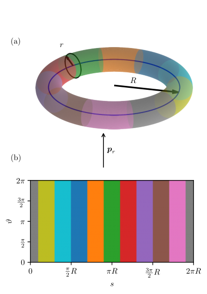
Using the relation of Eq. (6) we identify the linear topological charge density along a degeneracy line. Patterns (II) and (V) are degeneracy loops (ellipses), hence we can again surround any of them by a shrinking torus, described by the parametrization , where has the dimension of magnetic field (Tesla) and is dimensionless. For an isolated degeneracy point, the ground-state topological charge or Chern number associated to the point reads
| (7) |
where the integral is calculated for a closed surface enclosing the isolated degeneracy point, and is the Berry curvature vector field associated to the the ground-state wave function defined as
| (8) |
or writing component-wise
| (9) |
Therefore, for a degeneracy line, the formula revealing the linear topological charge density reads
| (10) |
This is the quantity that we study in the following.
For future reference, we introduce the two-dimensional (2D) Berry curvature via
| (11) |
i.e., the integrand in Eq. (10), and the apparent topological charge density , which is the right hand side of Eq. (10), without taking the limit :
| (12) |
related to the charge density defined above as
| (13) |
Since we use the Hamiltonian of Eq. (2) depending on dimensionless parameters as our starting point, all these newly introduced quantities are also dimensionless. Reinstating physical dimensions in Eq. (2) is done by multiplying the first term with the Bohr magneton and reinterpreting as a magnetic field and as an energy. Then, the physical dimension of the Berry curvature and the Berry flux density is magnetic field-2, whereas the dimension of the 2D Berry curvature, the apparent topological charge density and the topological charge density is magnetic field-1.
III.1 Pattern (II): neutral ellipse
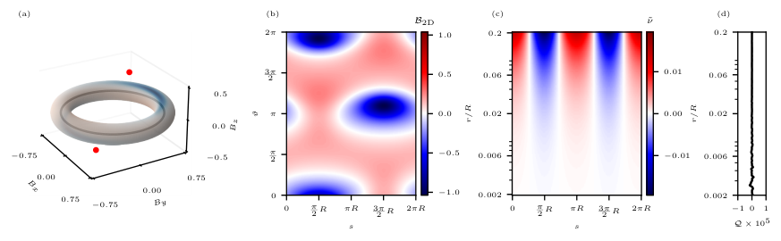
First we consider the neutral ellipse degeneracy pattern (II) in Fig. 1. For this pattern with zero total charge one can envision two qualitatively different scenarios: (a) The charge distribution is identically zero at all points of the ellipse. (b) There is a non-zero linear charge density along the ellipse, but the negative and positive contributions cancel each other when added up for the entire ellipse. Speculation based on classical electrostatics intuition actually suggest scenario (b): if we think of the ellipse as a globally charge-neutral ‘metal’, then the two point charges outside the ellipse would ‘polarize’ the ellipse.
In contrast, here we provide evidence that scenario (a) is the case, the local charge distribution along the degeneracy ellipse vanishes. This conclusion will be drawn from Fig. 3 c, but let us arrive there through a few intermediate steps.
In Fig. 3 a, we show the degeneracy patterns, two red points and a black ellipse. We use the specific choice of parameters where the -tensors are
| (14) |
and the exchange interaction is characterized by and . For simplicity, energy and magnetic field are dimensionless, unless noted otherwise.
The total topological charge carried by the red degeneracy points in Fig. 3 a is . These degeneracy points are located at opposite magnetic fields,
| (15) |
and each of them carry a topological charge . The degeneracy ellipse shown as the black loop in Fig. 3 is actually a circle in the plane for this parameter set, centered at the origin, with radius .
Figure 3 a shows the Berry flux density on a torus surrounding the degeneracy circle. The Berry flux density is defined as the normal-to-surface component of the Berry curvature vector field. For example, for a point on the torus, the Berry flux density reads
| (16) |
where is the normal vector of the torus at point . The torus in Fig. 3 a is colored according to the nonzero Berry flux density. (Numerical techniques to obtain Fig. 3 are described in Appendix B.)
On the way toward the linear topological charge density, to be expressed via Eq. (10), we specify the parametrization of the torus surrounding the degeneracy line as
| (17) |
with
Note that the normal vector of the torus can be expressed from the parametrization via
| (25) |
With the parametrization in Eq. (17), in Fig. 3 b we plot the 2D Berry curvature (see Eq. (11)) on the torus, with meridian radius . The data in Fig. 3 b is used to infer the linear topological charge density, by numerically performing the integration over the parameter and dividing by to obtain the apparent charge density , and then taking the limit . The apparent charge density as function of and is shown in Fig. 3 c. Although the value of the apparent charge density is nonzero for finite , it does converge to zero for all values of as . This is numerical evidence that the degeneracy circle is charge neutral. In section V we provide further analytical evidence to support this claim.
To illustrate the accuracy of our result shown in Fig. 3 c, we numerically evaluate the ground-state Chern number on the torus as the function of the meridian radius , by integrating the apparent charge density over the longitude path length . The result, shown in Fig. 3 d, is indeed zero, exhibiting a numerical error less than , illustrating that our numerical procedure is rather accurate.
III.2 Pattern (V): charged ellipse
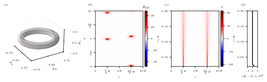
Next we consider the charged ellipse degeneracy pattern (V) in Fig. 1. The question is: how is the topological charge distributed along the ellipse? Using the method of the previous subsection, we show that the topological charge is concentrated at two opposite points of the ellipse, i.e. it is not continuously distributed along the ellipse.
The example parameter set we use consists of -tensors
| (26) |
and the interaction is described by and . The degeneracy ellipse is a circle with radius again, shown as a black line in Fig. 4 a.
Fig. 4 shows (a) the Berry flux density on a torus surrounding the degeneracy circle, (b) the two-dimensional Berry curvature on the pre-image of the torus, (c) the apparent topological charge density of the degeneracy circle, and (d) the numerically evaluated ground-state Chern number on the torus.
Fig. 4 a and b reveal a remarkable difference compared to Fig. 3 a and b: from Fig. 4 a and b, the Berry flux is concentrated in narrow regions (red spots) in the neighborhoods of two opposite points of the ellipse. Fig. 4 c suggests that the linear topological charge density, which corresponds to the plotted data in the limit, consists of two Dirac deltas: the degeneracy circle is neutral in all points except two discrete points opposite to each other, each carrying a topological charge of . In section V.1, this numerical evidence is supported by analytical results.
Fig. 4 d shows that the numerical error of the Chern number is below , illustrating the accuracy of our numerical procedure. The feature that the error grows as the radius decreases is rather natural: for smaller radius, the Berry flux gets more focused on a smaller area, hence our numerical integration using an equidistant grid on the pre-image of the torus gets less accurate.
The direction of the charged points is is , as determined by the Jordan decomposition of , according to Eq. (68). From Eq. (5), the position of these points is expressed as:
| (27) |
This result is in agreement with Fig. 4 c, where the charge density has two peaks at .
Figure 4 b shows pronounced peaks of the two-dimensional Berry curvature. These peaks appear because at each charged degeneracy point, there is a direction perpendicular to the degeneracy circle in which the energy splitting grows nonlinearly, and the Berry curvature peaks in those directions. For both degeneracy points, this direction, determined analytically using Eq. (95), is . This feature appears in the torus of Fig. 4b as which appears in Fig. 4 b as the regions where the flux density is high parametrized by the coordinates
| (28) |
matching the peaks seen in the numerical data.
To conclude, in this section we provided numerical evidence that the neutral degeneracy ellipse, pattern (II) of Frank et al. 2020, has vanishing linear topological charge density, whereas the charged degeneracy ellipse, pattern (V) of Frank et al. 2020, has all its topological charge focused in two opposite points of the ellipse. Even though the numerical results are obtained here for a specific choice of secondary parameters (-tensors, exchange strength and exchange rotation matrix ), the statements are general. For example, if the secondary parameters are changed with respect to those in section III.1, such that the resulting matrix still has the eigenpattern (II), then the degeneracy circle generically deforms into an ellipse, but all of its points remain charge-neutral. Results of section III.2 are generalized analogously. For details, we refer to Appendices C, D, and E.
IV Pattern (IV): continous surface charge distribution on an ellipsoid
Consider now the degeneracy pattern (IV) from Fig. 1, the charged ellipsoid. Again, we will follow the electrostatics analogy to determine the surface topological charge distribution on this ellipsoid, see also Ref. Souza et al. 2016. In electrostatics the surface charge density of surface and the electric field created by the surface charge density are related by the following formula:
| (29) |
where () is the normal component of the electric field outside (inside) the surface at point on the surface. Analogously, the surface topological charge density of the degeneracy ellipsoid is related to the Berry curvature vector field via
| (30) |
where is a point of the degeneracy surface.
Fig. 5 shows this surface topological charge distribution for the example parameter set with -tensors
| (31) |
and interaction described by and . In contrast to the result of section III.2, here we observe a continuous charge distribution. Figure 5 is obtained from our general result for the surface topological charge distribution, which reads
| (32) |
Here, is the diagonal element of the Jordan normal form of the matrix , which is Frank et al. 2020. Equation (32) is derived in Appendix G.
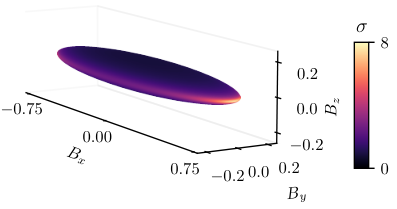
Interestingly, the surface charge density in Eq. (32) has the same functional form as the electrical charge distribution of an electrically charged conducting ellipsoid Curtright et al. 2020. Figure 5 exhibits the curvature effect known from electrostatics: the greater the curvature of the surface, the greater the topological charge density. A further similarity is that the Berry curvature inside the ellipsoid is zero, similarly to the electric field inside a charged ideal conductor. A difference, however, is that the Berry curvature in our example exits the surface radially with respect to the origin (i.e., it is proportional to ), in contrast to the electric field which exits the conductor’s surface in the surface normal direction (i.e., it is proportional to ). Another difference is that the curl of the Berry curvature is nonzero, however, the curl of the electric field induced by the charged conductor vanishes.
Given a degeneracy surface in a three-dimensional parameter space, is it a generic feature that it carries a continuous topological surface charge density? Here we argue that it is. Such a degeneracy surface divides the parameter space to two disjoint regions - in our example, the inside and the outside of the ellipsoid. The ground state changes continuously in both regions as the function of the parameters, generically implying a nonzero and continuous Berry curvature vector fields in both regions separately. But at the degeneracy surface, the ground state changes suddenly - in our example from a singlet-like state at the inside and a triplet-like state at the outside - and hence the Berry curvature also jumps, leading to a finite surface charge density according to Eq. (30).
V Discussion
V.1 Topological charge density vanishes for rank-2 points of degeneracy lines
In this section, we outline analytical results that support the numerical evidence of topological charge distributions studied in section III. To this end, we define the rank of degeneracy points, establish the ranks of the degeneracy points forming the linear degeneracy patterns studied in section III, and relate the rank of a degeneracy point to the topological charge of that point. In particular, we find that a rank-2 degeneracy point embedded in a linear degeneracy pattern carries no topological charge.
The effective -tensor of a degeneracy point is a real matrix that characterizes the Hamiltonian in the parameter-space vicinity of the degeneracy point , focusing on the two levels that are degenerate at the degeneracy point. Formally, we introduce the relative parameter vector measured from the degeneracy point, project the Hamiltonian to the two-dimensional ground-state subspace of the degeneracy point using an arbitrary orthonormal basis , and express that projected Hamiltonian in terms of Pauli matrices , e.g., , leading to the form Frank et al. 2020
| (33) |
Here, we have omitted the projected , since it is proportional to the unit matrix, owing to the degeneracy of the relevant two-dimensional subspace at . By the rank of a degeneracy point , we mean the matrix rank of the effective -tensor of that degeneracy point. Even though the effective -tensor depends on the choice of the basis , its determinant and rank do not.
In Appendix D.1, we show that all degeneracy points of the neutral degeneracy ellipse are rank 2. Furthermore, in Appendix D.2 we show that in the charged degeneracy ellipse, the two points where the Berry flux density is concentrated in Fig. 4 are rank 1, and all other degeneracy points are rank 2. Finally, in Appendix E, we prove that the linear topological charge density at a rank-2 degeneracy point of a line degeneracy is zero, supporting the numerical evidence seen in Figs. 3c and Figs. 4c. We also observe that the electrostatic analogy is not perfect: while the local charge density vanishes, hence there is no source of the Berry curvature on rank-2 degeneracy lines, there is always a linelike flux tube along the degeneracy, for details see Appendix E.
It is tempting to think about the charged ellipse degeneracy pattern (V) as a result of fine-tuning of pattern (II): upon tuning the secondary parameters (-tensors, exchange parameters), two charged points of pattern (II) merge with the neutral degeneracy ellipse of pattern (II), forming the charged degeneracy ellipse of pattern (V). (Note the related discussion on the conversion between Weyl point and nodal lines in band structures Sun et al. 2018.) This picture is reinforced by the fact that pattern (V) is less stable than pattern (II), signalled by their stability codimensions 4 and 3, respectively (see Table I. of Ref. Frank et al. 2020). Therefore, we conjecture that it is the generic behavior of two-fold degeneracy lines that their points have vanishing linear topological charge density. In other words, we conjecture that for , if a twofold line degeneracy has a point or segment with a nonzero linear topological charge density, then an infinitesimal perturbation, which preserves the line degeneracy but is generic otherwise, will separate the charge from the line degeneracy and render the latter locally neutral.
V.2 Symmetries can stabilize non-generic degeneracy patterns
Non-generic band degeneracy points and patterns in solids can be stabilized by the presence of symmetries Fang et al. 2012; Fang et al. 2016. Here, we show that interacting spin systems are similar: non-generic degeneracy points can be stabilized by symmetries.
We focus on a special case, when the two-spin system described by Eq. (2) has symmetry, and leave it for future work to explore further symmetry groups. We show that in this case, pattern (II) with two Weyl points and the neutral degeneracy circle is stabilized, even though it is unstable (codimension 3, see Table I in Ref. Frank et al. 2020) without the symmetry constraint.
Consider the case when the Hamiltonian is invariant under the isometries of the group , which are generated by the threefold rotation around the axis, and the reflection on the plane, . These isometries are represented by the matrices
| (34) |
and
| (35) |
on the pseudovectors (or axial vectors) appearing in the Hamiltonian of Eq. (2), i.e., the magnetic field and the electron spins and .
The presence of spatial symmetries is formalized as and . These conditions restrict the forms of , , and , in particular, , , and or . For concreteness, we still assume positive determinants for the -tensors, which implies .
Combining these symmetry constraints with the definition in Eq. (4) leads to , where and might be either positive or negative. This matrix is its own Jordan normal form, so we can directly apply the Jordan classification in Table I of Ref. Frank et al. 2020 to determine the degeneracy patterns arising in the magnetic parameter space. For , we find eigenpattern (VII), which has two Weyl points. For , we find eigenpattern (II), with two Weyl points and a neutral ellipse (circle, in this case), as studied in section III.1. Remarkably, as long as the symmetry is intact, the neutral ellipse survives without fine-tuning. In other words, the degeneracy pattern (II), which is unstable in the absence of symmetries, and hence is characterized by a positive codimension, becomes stable with zero codimension in the presence of symmetry.
VI Conclusions
We have exemplified the concepts of linear topological charge density and surface topological charge density through the example of a simple parameter-dependent quantum system, the spin-orbit-coupled two-spin problem where the paramters are the Cartesian components of the magnetic field acting on the spins. We have shown that the neutral degeneracy ellipse has vanishing topological charge density in all of its points, whereas the charged degeneracy ellipse has a charge distribution that is concentrated in two opposite points in the magnetic-field parameter space. Moreover, we have shown that the surface topological charge density of the degeneracy ellipse is continuous, and this charge density is identical to the surface charge density of a charged conducting ellipsoid. We have also shown that if the two-spin system has certain spatial symmetries, then this can stabilize an otherwise unstable, non-generic degeneracy pattern, e.g., a neutral circle.
The topological features described in this work have numerous physical consequences, e.g., they determine the experimentally measurable Berry curvature Schroer et al. 2014; Roushan et al. 2014, and also determine dynamical properties, such as paramagnetic resonance Koppens et al. 2006 or Landau–Zener-type processes Petta et al. 2010; Tanttu et al. 2019. Hence, we expect that our findings are testable in few-spin experiments, e.g., using quantum dots Scherübl et al. 2019; Veldhorst et al. 2015; Frank et al. 2020, molecular magnets Garg 2010; Wernsdorfer and Sessoli 1999; Bruno 2006 or adatoms on metallic surfaces Wiesendanger 2009; Spinelli et al. 2015.
Author contributions
Gy. F. and A. P. formulated the project and wrote the initial draft of the manuscript. A. P. acquired funding, and managed the project. Gy. F. performed analytical and numerical calculations with assistance from A. P. and D. V.. G. P. and P. V. consulted on differential-geometric aspects of the work. Gy. F. and D. V. produced the figures. All authors discussed the results and took part in writing the manuscript.
Acknowledgements.
We acknowledge fruitful discussions with G. Zaránd. This work was supported by the National Research Development and Innovation Office of Hungary within the Quantum Technology National Excellence Program (Project No. 2017-1.2.1-NKP-2017-00001), under OTKA Grants 124723, 132146, and under the BME Nanotechnology and Materials Science TKP2020 IE grant (BME IE-NAT TKP2020). D. V. was supported by NWO VIDI grant 680-47-53, the Swedish Research Council (VR) and the Knut and Alice Wallenberg Foundation.References
- Herring (1937) C. Herring, Accidental degeneracy in the energy bands of crystals, Phys. Rev. 52, 365 (1937).
- Berry (1984) M. V. Berry, Quantal phase factors accompanying adiabatic changes, Proceedings of the Royal Society of London A: Mathematical, Physical and Engineering Sciences 392, 45 (1984).
- Hasan and Kane (2010) M. Z. Hasan and C. L. Kane, Colloquium: Topological insulators, Rev. Mod. Phys. 82, 3045 (2010).
- Armitage et al. (2018) N. P. Armitage, E. J. Mele, and A. Vishwanath, Weyl and Dirac semimetals in three-dimensional solids, Rev. Mod. Phys. 90, 015001 (2018).
- Asbóth et al. (2016) J. K. Asbóth, L. Oroszlány, and A. Pályi, A Short Course on Topological Insulators (Springer, Heidelberg, 2016).
- Riwar et al. (2016) R.-P. Riwar, M. Houzet, J. S. Meyer, and Y. V. Nazarov, Multi-terminal Josephson junctions as topological matter, Nature Communications 7, 11167 (2016).
- Scherübl et al. (2019) Z. Scherübl, A. Pályi, G. Frank, I. E. Lukács, G. Fülöp, B. Fülöp, J. Nygård, K. Watanabe, T. Taniguchi, G. Zaránd, and S. Csonka, Observation of spin–orbit coupling induced Weyl points in a two-electron double quantum dot, Communications Physics 2, 108 (2019).
- Wernsdorfer and Sessoli (1999) W. Wernsdorfer and R. Sessoli, Quantum phase interference and parity effects in magnetic molecular clusters, Science 284, 133 (1999).
- Bruno (2006) P. Bruno, Berry phase, topology, and degeneracies in quantum nanomagnets, Phys. Rev. Lett. 96, 117208 (2006).
- Gritsev and Polkovnikov (2012) V. Gritsev and A. Polkovnikov, Dynamical quantum Hall effect in the parameter space, Proceedings of the National Academy of Sciences 109, 6457 (2012).
- Frank et al. (2020) G. Frank, Z. Scherübl, S. Csonka, G. Zaránd, and A. Pályi, Magnetic degeneracy points in interacting two-spin systems: Geometrical patterns, topological charge distributions, and their stability, Physical Review B 101, 245409 (2020).
- von Neumann and Wigner (1929) J. von Neumann and E. P. Wigner, Über das Verhalten von Eigenwerten bei adiabatischen Prozessen, Physikalische Zeitschrift 30, 467 (1929).
- Arnold (1995) V. I. Arnold, Remarks on eigenvalues and eigenvectors of Hermitian matrices, Berry phase, adiabatic connections and quantum Hall effect, Selecta Mathematica 1 (1995).
- Simon (1983) B. Simon, Holonomy, the quantum adiabatic theorem, and Berry’s phase, Phys. Rev. Lett. 51, 2167 (1983).
- Fang et al. (2012) C. Fang, M. J. Gilbert, X. Dai, and B. A. Bernevig, Multi-Weyl topological semimetals stabilized by point group symmetry, Phys. Rev. Lett. 108, 266802 (2012).
- Yan and Wang (2017) Z. Yan and Z. Wang, Floquet multi-Weyl points in crossing-nodal-line semimetals, Phys. Rev. B 96, 041206 (2017).
- Ahn et al. (2017) S. Ahn, E. J. Mele, and H. Min, Optical conductivity of multi-Weyl semimetals, Phys. Rev. B 95, 161112 (2017).
- Huang et al. (2017) Z.-M. Huang, J. Zhou, and S.-Q. Shen, Topological responses from chiral anomaly in multi-Weyl semimetals, Phys. Rev. B 96, 085201 (2017).
- Béri (2010) B. Béri, Topologically stable gapless phases of time-reversal-invariant superconductors, Phys. Rev. B 81, 134515 (2010).
- Carter et al. (2012) J.-M. Carter, V. V. Shankar, M. A. Zeb, and H.-Y. Kee, Semimetal and topological insulator in perovskite iridates, Phys. Rev. B 85, 115105 (2012).
- Fang et al. (2015) C. Fang, Y. Chen, H.-Y. Kee, and L. Fu, Topological nodal line semimetals with and without spin-orbital coupling, Phys. Rev. B 92, 081201 (2015).
- Wu et al. (2018) W. Wu, Y. Liu, S. Li, C. Zhong, Z.-M. Yu, X.-L. Sheng, Y. X. Zhao, and S. A. Yang, Nodal surface semimetals: Theory and material realization, Phys. Rev. B 97, 115125 (2018).
- Fang et al. (2016) C. Fang, H. Weng, X. Dai, and Z. Fang, Topological nodal line semimetals, Chinese Physics B 25, 117106 (2016).
- Bzdušek et al. (2016) T. Bzdušek, Q. Wu, A. Rüegg, M. Sigrist, and A. A. Soluyanov, Nodal-chain metals, Nature 538, 75 (2016).
- Liang et al. (2016) Q.-F. Liang, J. Zhou, R. Yu, Z. Wang, and H. Weng, Node-surface and node-line fermions from nonsymmorphic lattice symmetries, Phys. Rev. B 93, 085427 (2016).
- (26) Y.-M. Xie, X.-J. Gao, X. Y. Xu, C.-P. Zhang, J.-X. Hu, and K. T. Law, Kramers nodal line metals, arXiv:2008.03967 (unpublished).
- Kavokin (2004) K. V. Kavokin, Symmetry of anisotropic exchange interactions in semiconductor nanostructures, Phys. Rev. B 69, 075302 (2004).
- Kato et al. (2003) Y. Kato, R. C. Myers, D. C. Driscoll, A. C. Gossard, J. Levy, and D. D. Awschalom, Gigahertz electron spin manipulation using voltage-controlled g-tensor modulation, Science 299, 1201 (2003).
- Veldhorst et al. (2015) M. Veldhorst, R. Ruskov, C. H. Yang, J. C. C. Hwang, F. E. Hudson, M. E. Flatté, C. Tahan, K. M. Itoh, A. Morello, and A. S. Dzurak, Spin-orbit coupling and operation of multivalley spin qubits, Phys. Rev. B 92, 201401 (2015).
- Crippa et al. (2018) A. Crippa, R. Maurand, L. Bourdet, D. Kotekar-Patil, A. Amisse, X. Jehl, M. Sanquer, R. Laviéville, H. Bohuslavskyi, L. Hutin, S. Barraud, M. Vinet, Y.-M. Niquet, and S. De Franceschi, Electrical spin driving by -matrix modulation in spin-orbit qubits, Phys. Rev. Lett. 120, 137702 (2018).
- Schroer et al. (2011) M. D. Schroer, K. D. Petersson, M. Jung, and J. R. Petta, Field tuning the factor in inas nanowire double quantum dots, Phys. Rev. Lett. 107, 176811 (2011).
- (32) S. D. Liles, F. Martins, D. S. Miserev, A. A. Kiselev, I. D. Thorvaldson, M. J. Rendell, I. K. Jin, F. E. Hudson, M. Veldhorst, K. M. Itoh, O. P. Sushkov, T. D. Ladd, A. S. Dzurak, and A. R. Hamilton, Electrical control of the g-tensor of a single hole in a silicon MOS quantum dot, arXiv:2012.04985 (unpublished).
- Souza et al. (2016) T. Souza, M. Tomka, M. Kolodrubetz, S. Rosenberg, and A. Polkovnikov, Enabling adiabatic passages between disjoint regions in parameter space through topological transitions, Phys. Rev. B 94, 094106 (2016).
- Curtright et al. (2020) T. Curtright, Z. Cao, S. Huang, J. Sarmiento, S. Subedi, D. Tarrence, and T. Thapaliya, Charge densities for conducting ellipsoids, European Journal of Physics 41, 035204 (2020).
- Sun et al. (2018) X.-Q. Sun, S.-C. Zhang, and T. Bzdusek, Conversion rules for weyl points and nodal lines in topological media, Phys. Rev. Lett. 121, 106402 (2018).
- Schroer et al. (2014) M. D. Schroer, M. H. Kolodrubetz, W. F. Kindel, M. Sandberg, J. Gao, M. R. Vissers, D. P. Pappas, A. Polkovnikov, and K. W. Lehnert, Measuring a topological transition in an artificial spin- system, Phys. Rev. Lett. 113, 050402 (2014).
- Roushan et al. (2014) P. Roushan, C. Neill, Y. Chen, M. Kolodrubetz, C. Quintana, N. Leung, M. Fang, R. Barends, B. Campbell, Z. Chen, B. Chiaro, A. Dunsworth, E. Jeffrey, J. Kelly, A. Megrant, J. Mutus, P. J. J. O’Malley, D. Sank, A. Vainsencher, J. Wenner, T. White, A. Polkovnikov, A. N. Cleland, and J. M. Martinis, Observation of topological transitions in interacting quantum circuits, Nature 515, 241 (2014).
- Koppens et al. (2006) F. H. L. Koppens, C. Buizert, K. J. Tielrooij, I. T. Vink, K. C. Nowack, T. Meunier, L. P. Kouwenhoven, and L. M. K. Vandersypen, Driven coherent oscillations of a single electron spin in a quantum dot, Nature 442, 766 (2006).
- Petta et al. (2010) J. R. Petta, H. Lu, and A. C. Gossard, A coherent beam splitter for electronic spin states, Science 327, 669 (2010).
- Tanttu et al. (2019) T. Tanttu, B. Hensen, K. W. Chan, C. H. Yang, W. W. Huang, M. Fogarty, F. Hudson, K. Itoh, D. Culcer, A. Laucht, A. Morello, and A. Dzurak, Controlling spin-orbit interactions in silicon quantum dots using magnetic field direction, Phys. Rev. X 9, 021028 (2019).
- Garg (2010) A. Garg, Berry phases near degeneracies: Beyond the simplest case, Am. J. Phys. 78, 661 (2010).
- Wiesendanger (2009) R. Wiesendanger, Spin mapping at the nanoscale and atomic scale, Rev. Mod. Phys. 81, 1495 (2009).
- Spinelli et al. (2015) A. Spinelli, M. Gerrits, R. Toskovic, B. Bryant, M. Ternes, and A. F. Otte, Exploring the phase diagram of the two-impurity Kondo problem, Nature Communications 6, 10046 (2015).
- Horn and Johnson (1985) R. A. Horn and C. R. Johnson, Matrix Analysis (Cambridge, MA: Cambridge University Press, 1985).
Appendix A Proofs of Eq. (6)
A.1 First proof
In the main text, Eq. (6) expresses the linear charge density of a charged loop in terms of the electric field created by the loop. Here, we provide an elementary proof of that result.
Consider a cylindrical section of the torus, together with its top base and bottom base, surrounding a section of the degeneracy circle in Fig. 2 a. Without loss of generality, we can take the section defined by the interval with . From Gauss’ law, the total charge enclosed by the cylinder is expressed from the electric field as
| (36) | ||||
| Up to now, we assume that the cylinder has a nonzero meridian radius . Splitting up the cylinder’s surface integral to its three parts, we obtain | ||||
| (37) | ||||
| For , the top base and bottom base contributions converge to zero (see below), hence we find | ||||
| (38) | ||||
| Using the parametrization of the main text, this can be written as | ||||
| (39) | ||||
Assuming that the limit and the -integral can be exchanged, and considering that the boundaries of the integral were arbitrary, we arrive to Eq. (6).
In the remaining part of this subsection, we prove that the flux contributions of the top and bottom bases approach zero as the radius of the cylindrical section of the torus also approaches zero. To prove this, we consider a rather general setting depicted in Fig. 6. Here, the red curve is a charged wire, parametrized as by its path length , such that its left end corresponds to . The linear charge density of the wire is . Our goal is to show that the electric flux piercing the disk (blue) of radius at , chosen to be perpendicular to the wire, converges to zero as the radius approaches zero. This in turn ensures that the top-base and bottom-base integrals in the preceding paragraph vanish in the limit .

The flux created by a small line element of the charged wire between and is , where is the solid angle under which the disk is seen from the point , see Fig. 6. Without loss of generality, we assume that is positive. Then, the flux created by the charged wire is expressed as:
| (40) |
Here, is the path length parameter value corresponding to the right end of the wire, is the corresponding coordinate, and is the inverse function of the parametrization component which is assumed to be invertible. In the last step of Eq. (40), we substituted the integration variable by the coordinate, and accordingly, we introduced the modified linear charge density , which specifies the charge on the wire per unit distance along the axis.
Now we give an upper bound to the flux, by substituting the modified charge density by its maximum, :
| (41) |
We give a further, looser upper bound to the flux, by utilizing the relation between the solid angles of the points of the wire and the points of the axis, namely, , see Fig. 6:
| (42) |
Using , and performing a second change of variable by introducing the angle , see Fig. 6, we find:
| (43) |
As we decrease to zero, converges to , hence the second fraction converges to . Therefore, this upper bound converges to zero as , and hence the same is true for the flux .
A.2 Second proof
To give an alternative proof of the charge density formula (6), we start with the electrostatic field created by a linear charge density:
| (44) |
where is the parametrization of the line charge. For simplicity, we assume that the line charge is located along the axis. We justify this assumption a posteriori by the fact that the contribution of the charge distribution far from the point in question to the surface integral vanishes in the limit. If the degeneracy line is smooth, in the limit it is locally well approximated by a straight line.
Substituting this into the integral for a cylinder surrounding the charge density:
| (45) |
where . In the last step, we used that the fraction in the integrand converges to in the limit.
Appendix B Numerical techniques to obtain the figures
In this Appendix, we outline the numerical techniques we used to obtain Figs. 3 and 4 of the main text.
B.1 Berry flux density - Figs. 3 a and 4 a
Figs. 3 a and 4 a show the Berry flux density , defined via Eqs. (16) and (9), on the surface of the torus surrounding the circular degeneracy line. To obtain Fig. 3 a, our first step was to define a square grid on the parameter space, and the corresponding grid of points on the torus, obtained via the parametrization . The second step was to numerically approximate the derivatives in Eq. (9) on the grid points of the torus as
| (46) |
Here, , is the canonical unit vector pointing in direction , and we used . The gauge of the ground-state wave functions in the vicinity of a given was fixed such that the greatest-magnitude component of the four-component wave function was chosen to be real and positive. Having the Berry curvature vector field at hand, our final step was to evalute the Berry flux density by taking the normal projection in Eq. (16). The data shown in Fig. 4 a is obtained similarly.
B.2 2D Berry curvature - Figs. 3 b and 4 b
The 2D Berry curvature , plotted in Figs. 3 b and 4 b, is defined in Eq. (11) of the main text. We claim that this 2D Berry curvature is related to the Berry flux density discussed in the previous section via
| (47) |
Using this relation, we converted the data in Fig. 3 a (Fig. 4 a) to the data in Fig. 3 b (Fig. 4 b). The proof of Eq. (47) is straightforward: Eq. (25) is used at the right hand side of Eq. (11), then Eq. (16) is used, and finally the absolute value is evaluated using the specific parametrization in Eq. (17).
B.3 Apparent linear topological charge density - Figs. 3 c and 4 c
B.4 Chern number - Figs. 3 d and 4 d
Appendix C Jordan normal forms for the examples in the main text
In this section, we revisit the Jordan decomposition of real matrices, and discuss the relation between the matrix introduced in Eq. (4) of the main text, its Jordan decomposition, and the magnetic degeneracy points.
In the main text, we have introduced the real valued non-symmetric matrix in Eq. (4), as the central quantity of the two-spin problem. Also, we claimed that the directions of the degeneracy points are described by the left eigenvectors (left ordinary eigenvectors) of this matrix . Because of the non-symmetric property, is not always diagonalizable. Instead, it can be written as
which is called the Jordan decomposition Horn and Johnson 1985. Here, () is a non-singular matrix whose rows (columns) are the left (right) generalized eigenvectors of . From it follows that . It is important to note that the left (right) generalized eigenvectors are not necessarily orthogonal to each other and not necessarily normalized. Also, the transformation matrix is not unique. The matrix is the Jordan normal form of , which has a block-diagonal structure formed of Jordan blocks, matrices with the following structure:
| (62) |
where the diagonal elements are filled with the eigenvalue and the superdiagonal is composed of ones.
A left generalized eigenvector of rank corresponding to eigenvalue satisfies
| (63) | ||||
| and | ||||
| (64) | ||||
The parallel condition in Eq. (3) is fulfilled by the left ordinary eigenvectors denoted as which are the rank-1 generalized left eigenvectors. The th row in is an ordinary left eigenvector of if the th row in does not contain a superdiagonal 1 element. Linear combinations of ordinary eigenvectors corresponding to the same eigenvalue are also ordinary eigenvectors.
In the following subsections we provide the Jordan normal forms corresponding to the Hamiltonians and degeneracy patterns discussed in subsections III.1, and III.2, and section IV. Note that in these examples discussed in the main text, we set both the interaction matrix and the right -tensor as the unit matrix, and hence the matrix equals the left -tensor .
C.1 Degeneracy pattern (II), section III.1
For the example Hamiltonian producing the degeneracy pattern (II), treated in section III.1, the left -tensor was specified in Eq. (14), leading to
| (65) |
The matrices of the Jordan decomposition [see Eq. (C)] of this matrix read:
| (66) |
The Jordan normal form is diagonal, it consists of three Jordan blocks: two blocks of the form , and one block of the form .
As seen from Eqs. (C) and (66), the left eigenvector corresponding to the eigenvalue 4 is . As claimed in Eq. (15), there are two magnetic Weyl points, forming a time-reversed pair, along the B-field direction set by . It is also seen in Eq. (66) that two left eigenvectors corresponding to the eigenvalue 2 are and . In fact, all vectors in the subspace are eigenvectors with eigenvalue 2. According to Eqs. (5) and (14), the corresponding magnetic degeneracy points form a circle with radius .
C.2 Degeneracy pattern (V), section III.2
In section III.2, describing the charged ellipse degeneracy pattern (V), the left -tensor and hence the matrix was set to
| (67) |
A Jordan decomposition of this matrix is:
| (68) |
The Jordan normal form consists of the Jordan blocks and . There is a superdiagonal 1 element in the first row, hence is not an ordinary left eigenvector but a rank-2 generalized left eigenvector.
The ordinary eigenvectors are in the subspace similarly to the previous case. As a consequence of this, and Eq. (5), the corresponding degeneracies are on a circle with radius in the -plane again. This is similar to the degeneracy circle of pattern (II), but there the circle was neutral, while here it is charged.
Using Figs. 4 a,b,c, we argued in the main text that the topological charge of this charged degeneracy circle is localized on two opposite points of the circle. Here we claim that the charge is located in the direction. This can be illustrated by studying a parameter-dependent matrix that exemplifies a transition from the degeneracy pattern (II) formed by two equally-charged Weyl points and a neutral circle, to the degeneracy pattern (V) formed by the charged circle:
| (69) |
For , this matrix has a Jordan decomposition analogous to (66), i.e., it implies the degeneracy pattern (II). In particular, its largest eigenvalue is , with an ordinary left eigenvector . As is tuned continuously to zero, then coalesces with the (-independent) second left ordinary eigenvector . During this transition the Weyl points approach the neutral ellipse and then merge with it at .
C.3 Degeneracy pattern (IV), section IV
Appendix D Rank of the effective -tensor in the points of the degeneracy ellipses
Figure 3 of the main text provides numerical evidence that the topological charge density of the neutral degeneracy ellipse, of pattern (II), is zero. Similarly, Fig. 4 shows that the topological charge density of the charged degeneracy ellipse, pattern (V) is concentrated at two charged points, whereas the linear charge density in all other points of the ellipse is zero. In this section, we show that the above charge distributions are related to the ranks of the effective -tensors of the degeneracy points, defined in Eq. (33). Namely, the effective -tensor is a rank-1 matrix for the charged points of the charged ellipse, and a rank-2 matrix for the uncharged points of the charged ellipse and for every point of the neutral ellipse, too. The rank-2 property implies a first-order energy splitting of the degeneracy as we leave the degenerate line in any perpendicular direction. In the case of a rank-1 effective -tensor there exist a direction perpendicular to the plane of the degeneracy circle, with the property that the energy splitting is of higher-than-linear order if we leave the circle in that particular direction.
The effective -tensor for a ground-state degeneracy point at reads (Eq. (E11) of Ref. Frank et al. 2020)
| (71) |
where
| (72) |
Note that, here, we use a slightly different notation, compared to that in Ref. Frank et al. 2020: here we denote the dyadic product as a matrix product of a column vector and a row vector, instead of the alternative notation . The orthogonal matrix , which is defined [see Eq. (C2) of Ref. Frank et al. 2020] as an (ambiguous) rotation fulfilling , e.g., the rotation around the bisector of and .
Equation (71) for the effective -tensor is too complicated to determine directly. Instead, in the forthcoming calculation, we show that the rank is reflected by the rank of a a simpler matrix , which we express below in Eq. (87). Then, in subsections D.1 and D.2, we use this matrix to derive the rank of the effective -tensor on degeneracy ellipses.
As a first step in our calculation, we substitute with according to Eq. (72), into Eq. (71), and multiply the latter with from the right:
| (73) |
Here, we use instead of in the argument of , because the latter quantity does not depend on .
In cases (II) and (V), where degeneracy ellipses appear, the directions of the magnetic degeneracy points are in the subspace of the second and third left generalized eigenvectors. That is, the degeneracy points can be parameterized by the angle via
| (74) |
with . Since and are not necessarily orthogonal and normalized, is not necessarily and is not necessarily the angle between and .
The forthcoming steps lack an a priori intuitive justification, but a posteriori they prove to be particularly useful. First, let us recall that according to Eq. (C), the left generalized eigenvectors form the rows in the similarity transformation matrix in the Jordan decomposition of . Using this, can be written as the second row of the matrix , that is
| (75) |
where
| (76) |
Inserting a unit matrix in the form of to Eq. (75) yields
| (77) |
Here the sign denotes the definition of and in the last step, we used Eq. (C).
Substituting Eq. (77) to the effective -tensor of Eq. (73), we obtain
| (78) |
where we introduced the shorthand
| (79) |
which is a dyadic product.
Next, we further transform and in Eq. (78), starting with the latter. Substituting unit matrices into Eq. (79) yields
| (80) |
Then, using the associative nature of matrix multiplication, we obtain
| (81) |
where we introduced
| (82) |
Then, we substitute the definition of from Eq. (77) to Eq. (81), yielding
| (83) |
The denominator , which is the second vector component of , appears from the scalar product of with . Note that , which follows, e.g., from Eqs. (82) and (77), and it guarantees that the denominator in Eq. (83) is nonzero.
According to Eq. (83), the matrix can be thought of as a result of a similarity transformation generated by . Now, we transform the terms of Eq. (78) containing to a similar form. Multiplying with appropriately composed unit matrices, using its Jordan decomposition, and introducing the transformed Jordan normal form via
| (84) |
we find
| (85) |
Inserting Eqs. (83) and (85) into Eq. (78), we find the following expression for the effective -tensor:
| (86) |
where we introduced
| (87) |
Matrix has the same rank as the effective -tensor, because they only differ by multiplications of non-singular matrices. In what follows, we will determine the rank of the -tensor at the points of the degeneracy ellipses by determining the rank of .
D.1 Neutral ellipse
In Eq. (66), we have shown an example Jordan decomposition corresponding to a degeneracy pattern including a neutral ellipse. More generally, the normal form of that degeneracy pattern has a two-fold degeneracy of the following kind [see Table I of Ref. Frank et al. 2020]:
| (88) |
where and . Since its second Jordan block is proportional to the unit matrix, the transformation with defined in Eq. (76) leaves the normal form invariant:
| (89) |
for every . That means that every point of a neutral ellipse has the same rank effective -tensor. Then, expressing from Eqs. (87), (89) and (88) yields
| (90) |
cannot be a dyadic product because the condition cannot be satisfied as and . That means . The determinant of the effective -tensor is zero [Eq. (E23) of Ref. Frank et al. 2020 with ], therefore . This way we proved that the rank is 2 for every points of the neutral degeneracy ellipse.
D.2 Charged ellipse
In Eq. (68), we have shown an example for a Jordan decomposition corresponding to a degeneracy pattern of a charged ellipse. More generally, the Jordan normal form of that degeneracy pattern has a three-fold eigenvalue degeneracy, and a single 1 element in the superdiagonal:
| (91) |
with . Now does depend on the angle parameterizing the degeneracy point along the degeneracy ellipse:
| (92) |
Expressing from Eqs. (87) and (92) yields
| (93) |
where the elements and are given by lengthy but unimportant expressions. Similarly to the neutral ellipse, the condition is not satisfied for , hence the rank of the effective -tensor is 2 for those points. However, if , i.e., if the magnetic field is along the direction of , the matrix is clearly a dyadic product and not a zero matrix, hence its rank is 1, implying that the rank of the effective -tensor is also 1.
Finally, let us consider this latter case, when the rank of the effective -tensor is 1. Starting at the degeneracy point , and changing the magnetic field by along the degeneracy line as , the energy splitting induced by is at least of second order in . Since the rank of the effective -tensor is 1, there must be a plane of higher-order splitting, that is, a plane along which the energy splitting is at least of second order in . Which is the second direction, which spans this plane together with the direction of the degeneracy ellipse?
This question can be answered by recasting the rank-1 effective -tensor as a dyadic product of two vectors. Without the derivation, we claim that one way this can be done is as follows:
| (94) |
where
| (95) |
with is the right generalized eigenvector defined in Eq. (C). The column vector in the square bracket defines the direction of maximal linear splitting in , cf. Eq. (33). If lies in the plane perpendicular to that vector, then the energy splitting is at least second order in .
Appendix E Rank-2 points of a degeneracy line carry zero linear topological charge density
In this section, we show in general that degeneracy lines consisting of rank-2 points carry zero linear topological charge density. For simplicity, we assume that the degeneracy line is along the axis.
We use , and for brevity, and we shift the coordinate system of the magnetic parameter space such that the rank-2 point we consider is in the origin, where . From now on, we further simplify notation by using instead of (cf. Eq. (48)).
According to Eq. (12), our goal is to evaluate
| (96) |
For the parameter-space geometry we consider, the relation between the Cartesian coordinates and the torus parameters is , , and . Our strategy is to evaluate the above integral, i.e., to show that it vanishes, by using an approximate ground state for , obtained via a -dependent two-level effective Hamiltonian.
Along the axis, in the small neighborhood of the degeneracy point, we take an orthonormal basis of the degenerate ground-state subspace for each , such that the two basis states depend on continuously. Using this basis, we define the effective Hamiltonian of the degeneracy point as follows:
| (97) |
where projects on the two-dimensional ground-state subspace. (This projector should not be confused by the similarity transformation .) This effective Hamiltonian can also be written as
| (98) |
since our Hamiltonian [Eq. (2)] is a linear function of the magnetic field coordinates , , . Furthermore, by definition, projects to the twofold degenerate ground-state subspace of . Therefore, if we drop the degenerate part of the effective Hamiltonian, then we obtain
| (99) |
Up to now, the basis was ambigous, its defining constraints being that it has to depend continuously on , and it has to span the two-dimensional ground-state subspace of . Now, we further restrict this basis such that , , and . Then, the effective Hamiltonian is written as
| (100) |
with and . Note that the rank-2 character of the origin guarantees that .
This two-level effective Hamiltonian is straightforward to diagonalize, and its diagonalization provides a formula for the unique ground state away from the axis:
| (101) |
where is the angle enclosed by the vectors and . A key property of this angle is
| (102) |
implying
| (103) |
As we show below, this property implies , and hence a vanishing result of the integral in Eq. (96).
To compute the integrand of Eq. (96), we first evaluate the derivatives of the ground state (101):
| (104) | |||||
| (105) |
Then, the scalar product in the integrand of Eq. (96) reads
| (106) |
The second term in the square bracket is real, since
| (107) |
Furthermore, the third term is also real, since , defined as an angle, is real-valued.
As a consequence, the imaginary part of the scalar product in the integrand of Eq. (96) reads
| (108) |
From this result, it follows that
| (109) |
where we used Eqs. (102) and (103). Finally, Eq. (109) implies that the integral of Eq. (96) vanishes.
While the topological charge density vanishes at rank-2 points of a degeneracy line, the Berry curvature, even at an isolated degeneracy line, is not identically zero. To see this, we consider a small disk intersecting the degeneracy line and calculate the integral of the Berry connection around the perimeter of the disk, which is a loop surrounding the line degeneracy:
| (110) |
This result is independent of the radius of the disk chosen.
If the degeneracy is broken by some perturbation, the Berry curvature becomes well defined and finite everywhere, with a large Berry curvature along the position of the degeneracy line. In this case the integral of the Berry curvature for the disk equals the integral of the Berry connection around the perimeter
| (111) |
The connection integral changes continuously with perturbations of the Hamiltonian, while the curvature diverges at the degeneracy. This allows us to interpret this result in the degenerate case as half a quantum of Berry flux concentrated in a linelike flux tube along the line degeneracy.
Appendix F Example for finite linear topological charge density
In Eq. (10) we defined the linear topological charge density but showed later that it is either zero, or is concentrated to single points akin to a Dirac delta. Here, we provide an example Hamiltonian with a degeneracy line in its parameter space, such that the degeneracy line carries a finite, continuously-varying linear topological charge density.
Our example is a spin-1/2 Hamiltonian which is a nonlinear function of its parameters :
| (112) |
We will call the quantity the effective magnetic field. The Hamiltonian in Eq. (112) has a degeneracy line along the axis. For small but finite and/or , the degenerate ground state splits in energy, quadratically in and . To calculate the linear topological charge density of the degeneracy line along the axis, we follow the route introduced in section III, utilizing Eq. (10).
We consider a cylinder of finite radius surrounding the axis. We parametrize the points of this cylinder with cylindrical coordinates, via . At a given point of this cylinder, specified by , the effective magnetic field reads:
| (113) |
The ground state can be expressed as
| (114) |
where
| (115) | |||||
| (116) |
are the spherical angles of the effective magnetic field. For this specific Hamiltonian, these angles do not depend on the radius , hence the limit of Eq. (10) will be omitted below.
Having the - and -dependence of the ground state at hand, it is straightforward to calculate the two-dimensional Berry curvature according to Eq. (11):
| (117) |
which depends only on . From this, using Eq. (10), we evaluate the linear topological charge density:
| (118) |
which is indeed finite and depends continuously on the coordinate along the degeneracy line.
Appendix G Surface charge density of the charged ellipsoid
Here, we derive the surface charge density of the charged ellipsoid, a result quoted in the main text as Eq. (32). To do this, first, we transform the Hamiltonian to a simple form, where the Berry curvature is easy to determine, then we transform it back to obtain the surface charge density.
G.1 Berry curvature in a simplified Hamiltonian
The Hamiltonian introduced in Eq. (2) can be simplified with the following steps. A global unitary transformation which changes the right spin as changes the interaction to be isotropic
| (119) |
This transformation changes the right -tensor too. Now, we simplify the Zeeman term of the right spin with a linear transformation
| (120) |
To do this, we substitute the unit matrix , we get
| (121) |
This changes the left -tensor to a transformed matrix
| (122) |
The result is a Hamiltonian with and
| (123) |
The global unitary transformation leaves the Berry curvature invariant but the linear transformation in the parameter space changes it, as we derive it in the next subsection.
For degeneracy ellipsoids is proportional to the unit matrix,
| (124) |
The result is an isotropic Hamiltonian. It has a degeneracy sphere with radius
| (125) |
carrying a total topological charge 2. The Berry curvature in the transformed parameter space can be calculated using Gauss’s law because of the isotropy
| (126) |
G.2 Transformation of the Berry curvature in 3 dimensional parameter space
To obtain an isotropic Hamiltonian we did a global unitary transformation on the Hilbert space which preserves the Berry curvature, but we also did a linear transformation on the parameter space which, however, changes the curvature. In this subsection we derive the transformation of the Berry curvature in 3-dimensional parameter spaces.
We assume that Berry curvature with the transformed argument is known, this transformed curvature is given by where is the derivative with respect to . We want to find the curvature with respect to the variable , given by . For the th component we get
| (127) |
where we used the chain rule. The partial derivative is an element of the Jacobian matrix. This shows that the Berry curvature transforms as a 2-form. Multiplying with the Jacobian from the left yields
| (128) |
where the Berry curvature with the transformed argument appeared. From this we write the transformation rule specific to 3-dimensional parameter space:
| (129) |
For a linear transformation the Jacobian is the coefficient matrix.
G.3 Berry curvature in the parameter space of the ellipsoid
Now we can use the transformation of the Berry curvature derived in Eq. (129) to the Berry curvature in Eq. (126) with the transformation introduced in Eq. (120)
| (130) |
Here . Outside the ellipsoid we get
| (131) |
inside we get
| (132) |
From Eq. (5) we get the equation for the degeneracy ellipsoid
| (133) |
To get an expression for the surface normal of the ellipsoid, we consider the scalar field
| (134) |
that is constant on the degeneracy ellipsoid. Hence the gradient
| (135) |
is proportional to the normal vector of the surface. Thus, the normal vector for the degeneracy ellipsoid at reads
| (136) |
The surface topological charge density is proportional to the jump of the normal component of the Berry curvature
| (137) |
where in the last step Eq. (133) was used.