跳到论文正文
W Papers独立论文阅读器 arXiv:2012.14189 论文正文 计算阅读时间 · 0%
引用这篇论文根据当前论文元数据生成,正式投稿前建议核对。


License: CC Zero
arXiv:2012.14189v1 [math.CA] 28 Dec 2020

The two-dimensional fractional orthogonal derivative.

Enno Diekema Note: email adress: e.diekema@gmail.com
Abstract

This paper is an edited and shortened version of Chapter 6 from the thesis of the author [4]. First the one dimensional orthogonal derivative will be extended to the two-dimensional case. In the two-dimensional case we have to define the region of integration. In this paper we treat the integration over the square region and over the triangle region where in the last case we use biorthogonal polynomials expressed in terms of Appell functions. Next the two-dimensional orthogonal derivative will be extended to the two-dimensional fractional orthogonal derivative. The results are highly dependent on the F1F_{1}, F2F_{2} and F3F_{3} Appell functions.

1 Introduction

In Chapter 2 of the thesis of the author [4, Ch. 2] the orthogonal derivative of a function of one variable was defined. Just as this definition used orthogonal polynomials in one variable, we can try to approximate a partial derivative of a function in several variables by using orthogonal polynomials in several variables. In this paper we will consider the two-variable case. Similarly, we will extend the definition in [4, Ch. 3] of the fractional orthogonal derivative to the two-variable case.
The contents of this paper are as follows.
In section 2 we apply the method of [4, Ch. 2] to the two-variable case. We want to approximate ∂nf⁡(x,y)∂xn−k​∂yk\frac{\partial^{n}f(x,y)}{\partial x^{n-k}\partial y^{k}}. Only in the trivial case of a direct product of two orthogonality measures in one variable we can use fully orthogonal polynomials in two variables (again direct products) for this purpose. For other orthogonality measures on ℝ2\mathbb{R}^{2} we have to work with biorthogonal polynomials. The most obvious regions for the supports of these measures are the triangular region and the disk. We will only treat the triangular region with orthogonal measure already considered by Appell and yielding biorthogonal polynomials expressed in terms of Appell hypergeometric functions.

In section 3 we apply the theory of [4, Ch. 3] to the two-variable case, by which we obtain a two-dimensional fractional orthogonal derivative.

In section 4 we briefly treat the trivial case of the fractional Jacobi derivative with weight function on the square region.

In section 5 we treat the fractional biorthogonal derivative with weight function on the triangular region.

In the appendix we give an overview of the functions we need for the derivation of the formulas for the fractional orthogonal derivatives. We treat the F1F_{1}, F2F_{2}, F3F_{3} Appell functions, the H2H_{2} Horn function and the FPF_{P}, FQF_{Q} and the FP​RF_{PR} functions of Olsson.

2 The two-dimensional orthogonal derivatives

In [4, Ch. 2] we derived a formula for the orthogonal derivative

f(n)​(x)=kn​n!hn​limδ↓01δn​∫ℝf⁡(x+δ​u)​pn​(u)​𝑑μ​(u)f^{(n)}(x)=\dfrac{k_{n}n!}{h_{n}}\lim\limits_{\delta\downarrow 0}\dfrac{1}{\delta^{n}}\int\nolimits_{\mathbb{R}}f(x+\delta u)p_{n}(u)d\mu(u)

where the pnp_{n} are orthogonal polynomials. This formula can be considered, for instance, for Jacobi, Laguerre or Hermite polynomials. We can also use discrete orthogonal polynomials, for example the Hahn polynomials.

In the two-variable case we will work with Taylor series, as we did in the one-dimensional case, but now there is more freedom. Write the Taylor expansion of a function ff around (x,y)(x,y) as

f⁡(x+δ​u,y+δ​v)=δn​∑m=0n∑l=0m∂m∂xm−l​∂yl​f​(x,y)​um−l​vl(m−l)!​l!+o⁡(δn)f(x+\delta u,y+\delta v)=\delta^{n}\sum\limits_{m=0}^{n}\sum\limits_{l=0}^{m}\dfrac{\partial^{m}}{\partial x^{m-l}\partial y^{l}}f(x,y)\dfrac{u^{m-l}v^{l}}{(m-l)!\,l!}+o(\delta^{n}) (2.1)

where δ\delta is small. We want to approximate the partial derivative ∂n∂xn−k​∂yk​f​(x,y)\frac{\partial^{n}}{\partial x^{n-k}\partial y^{k}}f(x,y). For this purpose we look for a polynomial pn,k​(u,v)p_{n,k}(u,v) of degree nn such that, when both sides of (2.1) are multiplied by pn,k​(u,v)p_{n,k}(u,v) and next both sides are integrated over ℝ2\mathbb{R}^{2} with respect to a suitable orthogonality measure d​μ​(u,v)d\mu(u,v), all terms in the double summation except for the term with (m,l)=(n,k)(m,l)=(n,k) become zero. So first we want

∫ℝ∫ℝpn,k​(u,v)​um−l​vl​𝑑μ​(u,v)=0ifm<n\int\nolimits_{\mathbb{R}}\int\nolimits_{\mathbb{R}}p_{n,k}(u,v)u^{m-l}v^{l}d\mu(u,v)=0\qquad\text{if}\ \ m<n

This forces pn,kp_{n,k} to be in the (n+1n+1)-dimensional space 𝒱n{\cal V}_{n} of orthogonal polynomials of degree nn with respect to the measure μ\mu. Next we require that

∫ℝ∫ℝpn,k​(u,v)​un−l​vl​𝑑μ​(u,v)=0ifk≠l\int\nolimits_{\mathbb{R}}\int\nolimits_{\mathbb{R}}p_{n,k}(u,v)u^{n-l}v^{l}d\mu(u,v)=0\qquad\text{if}\ \ k\neq l (2.2)

This can be equivalently written as

∫ℝ2pn,k​(u,v)​qm,l​(u,v)​𝑑μ​(u,v)=0if(m,l)≠(n,k)\int_{\mathbb{R}^{2}}p_{n,k}(u,v)q_{m,l}(u,v)d\mu(u,v)=0\qquad\text{if}\ \ (m,l)\neq(n,k)

where the polynomials qn,lq_{n,l} are elements of 𝒱n{\cal V}_{n} such that qn,l​(u,v)=un−l​vlq_{n,l}(u,v)=u^{n-l}v^{l} + polynomial of degree less than nn. The polynomials qn,lq_{n,l} form the so-called monomial or monic basis of 𝒱n{\cal V}_{n}. The above condition on pn,k∈𝒱np_{n,k}\in{\cal V}_{n} now defines the polynomials pn,kp_{n,k} uniquely, up to a constant factor, as the basis of 𝒱n{\cal V}_{n} which is biorthogonal to the monomial basis. Then we get from (2.1) and the properties of pn,kp_{n,k} that

∂n∂xn−k​∂yk​f​(x,y)=(n−k)!​k!​limδ↓01δn​∫ℝ∫ℝf⁡(x+δ​u,y+δ​v)​pn,k​(u,v)​𝑑μ​(u,v)∫ℝ∫ℝpn,k​(u,v)​un−k​vk​𝑑μ​(u,v)\dfrac{\partial^{n}}{\partial x^{n-k}\partial y^{k}}f(x,y)=(n-k)!\,k!\lim\limits_{\delta\downarrow 0}\dfrac{1}{\delta^{n}}\dfrac{\int\nolimits_{\mathbb{R}}\int\nolimits_{\mathbb{R}}f(x+\delta u,y+\delta v)p_{n,k}(u,v)d\mu(u,v)}{\int\nolimits_{\mathbb{R}}\int\nolimits_{\mathbb{R}}p_{n,k}(u,v)u^{n-k}v^{k}d\mu(u,v)} (2.3)

under some conditions on ff, for instance that ff is a CnC^{n} function on some neighbourhood of (x,y)(x,y) and, if μ\mu has unbounded support, that |f⁡(u,v)||f(u,v)| tends sufficiently fast to 00 as (u,v)(u,v) tends to ∞\infty. More generally, we call the right-hand side of (2.3) a two-dimensional partial orthogonal derivative of ff at (x,y)(x,y) if the limit exists. But we will in particular be interested in the numerator on the right-hand side (after the limit sign) for fixed δ\delta. We will only treat the square and the triangular region. For the disk see [6, Section 5.2.2 with d=2d=2], [16, Chapter 3].

2.1 The two-dimensional Jacobi derivative with weight function on the square region

An easy example of (2.3) can be obtained by letting d​μ​(x,y)=d​μ1​(x)​d​μ2​(y)d\mu(x,y)=d\mu_{1}(x)d\mu_{2}(y) and pn,k​(x,y)=rn−k​(x)​sk​(y)p_{n,k}(x,y)=r_{n-k}(x)s_{k}(y) with the rnr_{n} and sns_{n} one-variable orthogonal polynomials for orthogonality measures μ1\mu_{1} and μ2\mu_{2}, respectively. Then the polynomials pn,kp_{n,k} are two-variable orthogonal polynomials for the orthogonality measure μ\mu while also pn,k​(x,y)=p_{n,k}(x,y)=Cxn−k​yk\,x^{n-k}y^{k} + polynomial of degree less than nn. So the pn,kp_{n,k} form the monomial basis, but this basis is also orthogonal, This is also biorthogonal to the monomial basis, by which the pn,kp_{n,k} are the polynomials desired in (2.3). Now the denominator after the limit sign on the right-hand side of (2.3) factorizes as the product

∫ℝrn−k​(u)​un−k​d​μ1​(u)×∫ℝsk​(v)​vk​d​μ2​(v)=hn−k′kn−k′​hk′′kk′′\int_{\mathbb{R}}r_{n-k}(u)u^{n-k}d\mu_{1}(u)\times\int_{\mathbb{R}}s_{k}(v)v^{k}d\mu_{2}(v)=\frac{h_{n-k}^{\prime}}{k_{n-k}^{\prime}}\frac{h_{k}^{\prime\prime}}{k_{k}^{\prime\prime}}

by [4, (2.2.4)], where the accented and double accented hnh_{n}’s and knk_{n}’s are in the obvious way, following [4, (2.2.3)], related to the orthogonal polynomials rnr_{n} and sns_{n}, respectively. Specialization of (2.3) gives:

∂m+n∂mx​∂ny​f​(x,y)=km​m!hm​kn​n!hn​limδ→01δm+n​∫−11∫−11f⁡(x+δ​v,y+δ​u)​pm​(u)​qn​(v)​𝑑μ​(u)​𝑑μ​(v)\dfrac{\partial^{m+n}}{\partial^{m}x\partial^{n}y}f(x,y)=\dfrac{k_{m}\,m!}{h_{m}}\dfrac{k_{n}\,n!}{h_{n}}\lim\limits_{\delta\rightarrow 0}\dfrac{1}{\delta^{m+n}}\int\nolimits_{-1}^{1}\int\nolimits_{-1}^{1}f(x+\delta v,y+\delta u)p_{m}(u)q_{n}(v)d\mu(u)d\mu(v) (2.4)

This is a very trivial case. If the measures μ1\mu_{1} and μ2\mu_{2} are supported on the segment [−1,1][-1,1] then the polynomials pn,kp_{n,k} are orthogonal on the square [−1,1]×[−1,1][-1,1]\times[-1,1]. For example, take the product of the Jacobi measures d​μ1​(x)=(1−x)α​(1+x)β​d​xd\mu_{1}(x)=(1-x)^{\alpha}(1+x)^{\beta}dx and d​μ2​(y)=(1−y)γ​(1+y)δ​d​yd\mu_{2}(y)=(1-y)^{\gamma}(1+y)^{\delta}dy. Substitution in (2.4) gives at last

∂n+k∂xn​∂yk​f​(x,y)=limδ→01δn+k​kn,α,β​kk,γ,δhn,α,β​hk,γ,δ×∫−11∫−11f⁡(x+δ​u,y+δ​v)​Pn(α,β)​(u)​Pk(γ,δ)​(v)​(1−u)α​(1+u)β​(1−v)γ​(1+v)δ​𝑑u​𝑑v\dfrac{\partial^{n+k}}{\partial x^{n}\partial y^{k}}f(x,y)=\lim\limits_{\delta\rightarrow 0}\dfrac{1}{\delta^{n+k}}\dfrac{k_{n,\alpha,\beta}\ k_{k,\gamma,\delta}}{h_{n,\alpha,\beta}\ h_{k,\gamma,\delta}}\\ \times\int\nolimits_{-1}^{1}\int\nolimits_{-1}^{1}f(x+\delta u,y+\delta v)P_{n}^{(\alpha,\beta)}(u)P_{k}^{(\gamma,\delta)}(v)(1-u)^{\alpha}(1+u)^{\beta}(1-v)^{\gamma}(1+v)^{\delta}\,du\,dv

2.2 The two-dimensional biorthogonal derivative with weight function on the triangular region

The triangular region of ℝ2{\mathbb{R}}^{2} is defined as T2:={(x,y):0≤x,y≤1∧x+y≤1}T^{2}:=\left\{(x,y):0\leq x,y\leq 1\wedge x+y\leq 1\right\}, on which we consider the Jacobi weight function defined as:

Wα,β,γ​(x,y):=1B⁡(α+1,β+1,γ+1)​xα​yβ​(1−x−y)γα,β,γ>−1W_{\alpha,\beta,\gamma}(x,y):=\dfrac{1}{B(\alpha+1,\beta+1,\gamma+1)}x^{\alpha}y^{\beta}(1-x-y)^{\gamma}\qquad\alpha,\beta,\gamma>-1

which is normalized in such a way that its integral over T2T^{2} is 11. The function B⁡(x,y,z)B(x,y,z) is defined as an extension of the Beta function

B⁡(x,y,z):=Γ⁡(x)​Γ​(y)​Γ​(z)Γ⁡(x+y+z)B(x,y,z):=\dfrac{\Gamma(x)\Gamma(y)\Gamma(z)}{\Gamma(x+y+z)}

It is easy to prove

B⁡(x,y,z)=B⁡(x,y+z)​B​(y,z)=B⁡(y,x+z)​B​(x,z)=B⁡(z,x+y)​B​(x,y)B(x,y,z)=B(x,y+z)B(y,z)=B(y,x+z)B(x,z)=B(z,x+y)B(x,y)

Let

⟨f,g⟩α,β,γ=∫T2f⁡(x,y)​g​(x,y)​Wα,β,γ​(x,y)​𝑑x​𝑑y\left\langle f,g\right\rangle_{\alpha,\beta,\gamma}=\int\nolimits_{T^{2}}f(x,y)g(x,y)W_{\alpha,\beta,\gamma}(x,y)\;dx\;dy

Classical orthogonal polynomials of one variable all satisfy a Rodrigues’ formula. For obtaining something similar in connection with the triangular region Appell considered the following analogue of Rodrigues’ formula [6, Section 2.4]:

Uk,nα,β,γ​(x,y)=[xα​yβ​(1−x−y)γ]−1​∂n∂xk​∂yn−k​[xk+α​yn−k+β​(1−x−y)n+γ]0≤k≤nU_{k,n}^{\alpha,\beta,\gamma}(x,y)=\big[x^{\alpha}y^{\beta}(1-x-y)^{\gamma}\big]^{-1}\dfrac{\partial^{n}}{\partial x^{k}\partial y^{n-k}}\left[x^{k+\alpha}y^{n-k+\beta}(1-x-y)^{n+\gamma}\right]\qquad 0\leq k\leq n (2.5)

The set {Uk,nα,β,γ​(x,y):0≤k≤n}\{U_{k,n}^{\alpha,\beta,\gamma}(x,y):0\leq k\leq n\} is a basis of 𝒱n2​(Wα,β,γ)\mathcal{V}_{n}^{2}(W_{\alpha,\beta,\gamma}) where 𝒱n2\mathcal{V}_{n}^{2}  is the space of orthogonal polynomials of degree nn. See [6, Prop. 2.4.3].

To write Uk,nα,β,γ​(x,y)U_{k,n}^{\alpha,\beta,\gamma}(x,y) as an F2F_{2} Appell function we can use [7, 5.13(1)]. There follows:

Uk,nα,β,γ​(x,y)=(α+1)k​(β+1)n−k​(1−x−y)nF2​(−γ−n,−k,−n+k,α+1,β+1,xx+y−1,yx+y−1)U_{k,n}^{\alpha,\beta,\gamma}(x,y)=(\alpha+1)_{k}(\beta+1)_{n-k}(1-x-y)^{n}\\ F_{2}\left(-\gamma-n;-k,-n+k;\alpha+1,\beta+1;\dfrac{x}{x+y-1},\dfrac{y}{x+y-1}\right)

From this expression we see that Uk,nα,β,γ​(x,y)U_{k,n}^{\alpha,\beta,\gamma}(x,y) are polynomials of degree less or equal nn. Using [7, 5.11(8)] we get the much simpler form

Uk,nα,β,γ​(x,y)=(α+1)k​(β+1)n−k​(1−x−y)−γF2​(−γ−n,α+1+k,β+1+n−k,α+1,β+1,x,y)U_{k,n}^{\alpha,\beta,\gamma}(x,y)=(\alpha+1)_{k}(\beta+1)_{n-k}(1-x-y)^{-\gamma}\\ F_{2}(-\gamma-n;\alpha+1+k,\beta+1+n-k;\alpha+1,\beta+1;x,y) (2.6)

This basis is not orthogonal. It can be shown that ⟨Uk,nα,β,γ,Uj,nα,β,γ⟩α,β,γ≠0\left\langle U_{k,n}^{\alpha,\beta,\gamma},U_{j,n}^{\alpha,\beta,\gamma}\right\rangle_{\alpha,\beta,\gamma}\neq 0 for j≠kj\neq k. If n≠mn\neq m then ⟨Uk,nα,β,γ,Uj,mα,β,γ⟩α,β,γ=0\left\langle U_{k,n}^{\alpha,\beta,\gamma},U_{j,m}^{\alpha,\beta,\gamma}\right\rangle_{\alpha,\beta,\gamma}=0.

Let Vm,nα,β,γV_{m,n}^{\alpha,\beta,\gamma} be defined with 0≤m≤n0\leq m\leq n by

Vm,nα,β,γ​(x,y):==∑i=0m∑j=0n(−1)m+n+i+j​(mi)​(nj)​(α+1)m​(β+1)n​(α+β+γ+2)m+n+i+j(α+1)i​(β+1)j​(α+β+γ+2)2​m+2​n​xi​yjV_{m,n}^{\alpha,\beta,\gamma}(x,y):=\\ =\sum\limits_{i=0}^{m}\sum\limits_{j=0}^{n}(-1)^{m+n+i+j}\dbinom{m}{i}\dbinom{n}{j}\dfrac{(\alpha+1)_{m}(\beta+1)_{n}(\alpha+\beta+\gamma+2)_{m+n+i+j}}{(\alpha+1)_{i}(\beta+1)_{j}(\alpha+\beta+\gamma+2)_{2m+2n}}x^{i}y^{j} (2.7)

This function can be written as an F2F_{2} Appell function.

Vm,nα,β,γ​(x,y)=(−1)n+m​(α+1)m​(β+1)n​(α+β+γ+2)m+n(α+β+γ+2)2​n+2​mF2​(α+β+γ+2+m+n,−m,−n,α+1,β+1,x,y)V_{m,n}^{\alpha,\beta,\gamma}(x,y)=(-1)^{n+m}\dfrac{(\alpha+1)_{m}(\beta+1)_{n}(\alpha+\beta+\gamma+2)_{m+n}}{(\alpha+\beta+\gamma+2)_{2n+2m}}\\ F_{2}(\alpha+\beta+\gamma+2+m+n;-m,-n;\alpha+1,\beta+1;x,y) (2.8)

Then Vm,nV_{m,n} is the orthogonal projection of xm​ynx^{m}y^{n} in L2​⟨T2,Wμ⟩L^{2}\left\langle T^{2},W_{\mu}\right\rangle onto the space 𝒱m+n\mathcal{V}_{m+n} of orthogonal polynomials of degree m+nm+n (so they are a monomial basis) and the two families of polynomials are biorthogonal with

⟨Uk,nα,β,γ,Vj,n−jα,β,γ⟩α,β,γ=(−1)n​(α+1)k​(β+1)n−k​(γ+1)n​k!​(n−k)!(α+β+γ+3)2​n​δj,k0≤j,k≤n\left\langle U_{k,n}^{\alpha,\beta,\gamma},V_{j,n-j}^{\alpha,\beta,\gamma}\right\rangle_{\alpha,\beta,\gamma}=(-1)^{n}\dfrac{(\alpha+1)_{k}(\beta+1)_{n-k}(\gamma+1)_{n}k!\,(n-k)!}{(\alpha+\beta+\gamma+3)_{2n}}\delta_{j,k}\qquad 0\leq j,k\leq n (2.9)

We can write this last inner product more generally by replacing the parameter n−jn-j by m−jm-j. There follows

⟨Uk,nα,β,γ,Vj,m−jα,β,γ⟩α,β,γ=0m≠n\left\langle U_{k,n}^{\alpha,\beta,\gamma},V_{j,m-j}^{\alpha,\beta,\gamma}\right\rangle_{\alpha,\beta,\gamma}=0\qquad m\neq n

The basis of polynomials Vm,nα,β,γV_{m,n}^{\alpha,\beta,\gamma} as well as the above biorthogonality is already given by Appell for γ=0\gamma=0 and by Fackerel & Littler [9] for the general case. If we compare with the notation for the general case at the beginning of Section 2 then we see that Uk,nα,β,γ=pn,n−kU_{k,n}^{\alpha,\beta,\gamma}=p_{n,n-k} and Vl,m−lα,β,γ=qm,m−lV_{l,m-l}^{\alpha,\beta,\gamma}=q_{m,m-l}. Hence, for the partial orthogonal derivative (2.3) we have to use the UU-basis in the present case.

Using the triangular region T2={(x,y):0≤x,y,x+y<1}T^{2}=\left\{(x,y):0\leq x,y,x+y<1\right\} we get for the denominator of (2.3)

I⁡(m,l)\displaystyle I(m,l) =∬0≤u,v,u+v<1Uk,nα,β,γ​(u,v)​um−l​vl​Wα,β,γ​(u,v)​𝑑u​𝑑v=\displaystyle=\iint\nolimits_{0\leq u,v,u+v<1}U_{k,n}^{\alpha,\beta,\gamma}(u,v)u^{m-l}v^{l}W_{\alpha,\beta,\gamma}(u,v)dudv=
=[B⁡(α+1,β+1,γ+1)]−1\displaystyle=\big[B(\alpha+1,\beta+1,\gamma+1)\big]^{-1}
×∫01vl​∫01−vum−l​∂k∂uk​∂n−k∂vn−k​[uk+α​vn−k+β​(1−u−v)n+γ]​𝑑u​𝑑v\displaystyle\qquad\qquad\times\int\nolimits_{0}^{1}v^{l}\int\nolimits_{0}^{1-v}u^{m-l}\dfrac{\partial^{k}}{\partial u^{k}}\dfrac{\partial^{n-k}}{\partial v^{n-k}}\left[u^{k+\alpha}v^{n-k+\beta}(1-u-v)^{n+\gamma}\right]\,du\,dv (2.10)

By integration by parts with respect to uu we see that I⁡(m,l)=0I\left(m,l\right)=0 unless l+k≤ml+k\leq m. By integration by parts with respect to vv we see that I⁡(m,l)=0I(m,l)=0 unless n≤l+kn\leq l+k. Together with m≤nm\leq n there follows: m=nm=n and l=n−kl=n-k. Substitution in (2.10) gives

I⁡(n,n−k)\displaystyle I(n,n-k) B⁡(α+1,β+1,γ+1)=\displaystyle B(\alpha+1,\beta+1,\gamma+1)=
=∫01vn−k​∫01−vuk​∂k∂uk​∂n−k∂vn−k​[uk+α​vn−k+β​(1−u−v)n+γ]​𝑑u​𝑑v\displaystyle=\int\nolimits_{0}^{1}v^{n-k}\int\nolimits_{0}^{1-v}u^{k}\dfrac{\partial^{k}}{\partial u^{k}}\dfrac{\partial^{n-k}}{\partial v^{n-k}}\left[u^{k+\alpha}v^{n-k+\beta}(1-u-v)^{n+\gamma}\right]\,du\,dv (2.11)

Let

I1=∫01−vuk​∂k∂uk​[∂n−k∂vn−k​[uk+α​vn−k+β​(1−u−v)n+γ]]​𝑑uI_{1}=\int\nolimits_{0}^{1-v}u^{k}\dfrac{\partial^{k}}{\partial u^{k}}\left[\dfrac{\partial^{n-k}}{\partial v^{n-k}}\left[u^{k+\alpha}v^{n-k+\beta}(1-u-v)^{n+\gamma}\right]\right]\,du

After kk-fold integration by parts there remains

I1=(−1)k​Γ​(k+1)​∫01−vuk+α​∂n−k∂vn−k​[vn−k+β​(1−u−v)n+γ]​𝑑uI_{1}=(-1)^{k}\Gamma(k+1)\int\nolimits_{0}^{1-v}u^{k+\alpha}\dfrac{\partial^{n-k}}{\partial v^{n-k}}\left[v^{n-k+\beta}(1-u-v)^{n+\gamma}\right]du

Substitution in (2.11) gives

I⁡(n,n−k)\displaystyle I(n,n-k) [(−1)k​Γ​(k+1)]−1​B​(α+1,β+1,γ+1)=\displaystyle\big[(-1)^{k}\Gamma(k+1)\big]^{-1}B(\alpha+1,\beta+1,\gamma+1)=
=∫01vn−k​∫01−vuk+α​∂n−k∂vn−k​[vn−k+β​(1−u−v)n+γ]​𝑑u​𝑑v\displaystyle=\int\nolimits_{0}^{1}v^{n-k}\int\nolimits_{0}^{1-v}u^{k+\alpha}\dfrac{\partial^{n-k}}{\partial v^{n-k}}\left[v^{n-k+\beta}(1-u-v)^{n+\gamma}\right]\,du\,dv
=∫01uk+α​∫01−uvn−k​∂n−k∂vn−k​[vn−k+β​(1−u−v)n+γ]​𝑑v​𝑑u\displaystyle=\int\nolimits_{0}^{1}u^{k+\alpha}\int\nolimits_{0}^{1-u}v^{n-k}\dfrac{\partial^{n-k}}{\partial v^{n-k}}\left[v^{n-k+\beta}(1-u-v)^{n+\gamma}\right]\,dv\,du (2.12)

Let

I2=∫01−uvn−k​∂n−k∂vn−k​[vn−k+β​(1−u−v)n+γ]​𝑑vI_{2}=\int\nolimits_{0}^{1-u}v^{n-k}\dfrac{\partial^{n-k}}{\partial v^{n-k}}\left[v^{n-k+\beta}(1-u-v)^{n+\gamma}\right]\,dv

After (n−k)(n-k)-fold integration by parts we get

I2=(−1)n−k​Γ​(n−k+1)​∫01−uvn−k+β​(1−u−v)n+γ​𝑑vI_{2}=(-1)^{n-k}\Gamma(n-k+1)\int\nolimits_{0}^{1-u}v^{n-k+\beta}(1-u-v)^{n+\gamma}dv

The integral is a Beta function.

∫01−uvn−k+β​(1−u−v)n+γ​𝑑v=(1−u)k+2​n+β+γ+1​B​(n−k+β+1,n+γ+1)\int\nolimits_{0}^{1-u}v^{n-k+\beta}(1-u-v)^{n+\gamma}dv=(1-u)^{k+2n+\beta+\gamma+1}B(n-k+\beta+1,n+\gamma+1)

with convergence conditions: β,γ>−1\beta,\gamma>-1. So for I2I_{2} we get

I2=(−1)n−k​Γ​(n−k+1)​(1−u)k+2​n+β+γ+1​B​(n−k+β+1,n+γ+1)I_{2}=(-1)^{n-k}\Gamma(n-k+1)(1-u)^{k+2n+\beta+\gamma+1}B(n-k+\beta+1,n+\gamma+1)

Substitution in (2.12) gives

I⁡(n,n−k)​[(−1)n​Γ​(k+1)​Γ​(n−k+1)]−1​B​(α+1,β+1,γ+1)==B⁡(n−k+β+1,n+γ+1)​∫01uk+α​(1−u)k+2​n+β+γ+1​𝑑uI(n,n-k)\big[(-1)^{n}\Gamma(k+1)\Gamma(n-k+1)\big]^{-1}B(\alpha+1,\beta+1,\gamma+1)=\\ =B(n-k+\beta+1,n+\gamma+1)\int\nolimits_{0}^{1}u^{k+\alpha}(1-u)^{k+2n+\beta+\gamma+1}du

The integral is again a Beta function. So we get

I(n,n−k)[(−1)n\displaystyle I(n,n-k)\big[(-1)^{n} Γ(k+1)Γ(n−k+1)]−1B(α+1,β+1,γ+1)=\displaystyle\Gamma(k+1)\Gamma(n-k+1)\big]^{-1}B(\alpha+1,\beta+1,\gamma+1)=
=B⁡(n−k+β+1,n+γ+1)​B​(k+α+1,2​n−k+β+γ+2)\displaystyle=B(n-k+\beta+1,n+\gamma+1)B(k+\alpha+1,2n-k+\beta+\gamma+2)
=B⁡(k+α+1,n−k+β+1,n+γ+1)\displaystyle=B(k+\alpha+1,n-k+\beta+1,n+\gamma+1)

with convergence conditions: Re⁡α,Re⁡β,Re⁡γ>−1\operatorname{Re}{\alpha},\operatorname{Re}{\beta},\operatorname{Re}{\gamma}>-1. After some manipulations we get

I⁡(n,n−k)=(−1)n​(α+1)k​(β+1)n−k​(γ+1)n​k!​(n−k)!(α+β+γ+3)2​nI(n,n-k)=(-1)^{n}\dfrac{(\alpha+1)_{k}(\beta+1)_{n-k}(\gamma+1)_{n}k!\,(n-k)!}{(\alpha+\beta+\gamma+3)_{2n}}

and this is equal to the constant in (2.9). This also follows from the fact that

I⁡(n,n−k)\displaystyle I(n,n-k) =<Uk,n,uk​vn−k>\displaystyle=<U_{k,n},\,u^{k}\,v^{n-k}>
=<Uk,n,Vk,n−k+polynomial of degree less than n>\displaystyle=<U_{k,n},\,V_{k,n-k}+\text{polynomial of degree less than $n$}>
=<Uk,n,Vk,n−k>+<Uk,n,polynomial of degree less than n>\displaystyle=<U_{k,n},\,V_{k,n-k}>+<U_{k,n},\text{polynomial of degree less than $n$}>
=<Uk,n,Vk,n−k>\displaystyle=<U_{k,n},\,V_{k,n-k}>

Substitution in (2.3) gives

∂n∂xk​∂yn−k​f​(x,y)=(−1)nB⁡(α+1+k,β+1+n−k,γ+1+n)limδ↓01δn​∬0≤u,v,u+v<1f⁡(x+δ​u,y+δ​v)​Uk,nα,β,γ​(u,v)​uα​vβ​(1−u−v)γ​𝑑v​𝑑u\dfrac{\partial^{n}}{\partial x^{k}\partial y^{n-k}}f(x,y)=\dfrac{(-1)^{n}}{B(\alpha+1+k,\beta+1+n-k,\gamma+1+n)}\\ \lim\limits_{\delta\downarrow 0}\dfrac{1}{\delta^{n}}\iint\nolimits_{0\leq u,v,u+v<1}f(x+\delta u,y+\delta v)U_{k,n}^{\alpha,\beta,\gamma}(u,v)u^{\alpha}v^{\beta}(1-u-v)^{\gamma}\,dv\,du (2.13)

with convergence conditions: α,β,γ>−1\alpha,\beta,\gamma>-1. Using (2.6) gives

∂n∂xk​∂yn−k​f​(x,y)=(−1)n​Γ​(α+β+γ+3+2​n)Γ⁡(α+1)​Γ​(β+1)​Γ​(γ+1+n)limδ↓01δn​∬0≤u,v,u+v<1f⁡(x+δ​u,y+δ​v)​F2​(−γ−n;α+1+k,β+1+n−kα+1,β+1,u,v)​uα​vβ​𝑑v​𝑑u\dfrac{\partial^{n}}{\partial x^{k}\partial y^{n-k}}f(x,y)=\dfrac{(-1)^{n}\Gamma(\alpha+\beta+\gamma+3+2n)}{\Gamma(\alpha+1)\Gamma(\beta+1)\Gamma(\gamma+1+n)}\\ \lim\limits_{\delta\downarrow 0}\dfrac{1}{\delta^{n}}\iint\nolimits_{0\leq u,v,u+v<1}f(x+\delta u,y+\delta v)F_{2}\left(\begin{array}[]{c}-\gamma-n;\alpha+1+k,\beta+1+n-k\\ \alpha+1,\beta+1\end{array};u,v\right)u^{\alpha}v^{\beta}\,dv\,du

3 The two-dimensional fractional orthogonal derivative

We have seen that for the orthogonal derivative in two dimensions there are several choices of region and orthogonality measures for which explicit results can be obtained. For the fractional derivative in two dimensions we have the same possibilities. So we treat first the trivial case of the fractional orthogonal derivative with weight function on the square. Then we treat the fractional biorthogonal derivative with weight function on the triangular region.

Analogous to the Weyl fractional integral in one dimension we define the Weyl fractional integral in two dimensions as:

W−μ,−ν​[f]​(x,y):=1Γ⁡(μ)​Γ​(ν)​∫x∞∫y∞f⁡(U,V)​(U−x)μ−1​(V−y)ν−1​𝑑V​𝑑UW^{-\mu,-\nu}[f](x,y):=\dfrac{1}{\Gamma(\mu)\Gamma(\nu)}\int\nolimits_{x}^{\infty}\int\nolimits_{y}^{\infty}f(U,V)(U-x)^{\mu-1}(V-y)^{\nu-1}dVdU

The fractional partial derivative will be given by

Wμ,ν[f](x,y)=(−1)m∂m∂xm−l​∂ylWμ−m+l,ν−l[f](x,y)=(−1)mΓ⁡(m−l−μ)​Γ​(l−ν)​∂m∂xm−l​∂yl​[∫x∞∫y∞f⁡(U,V)​(U−x)m−l−μ−1​(V−y)l−ν−1​𝑑V​𝑑U]W^{\mu,\nu}[f](x,y)=(-1)^{m}\dfrac{\partial^{m}}{\partial x^{m-l}\partial y^{l}}W^{\mu-m+l,}{}^{\nu-l}[f](x,y)\\ =\dfrac{(-1)^{m}}{\Gamma(m-l-\mu)\Gamma(l-\nu)}\dfrac{\partial^{m}}{\partial x^{m-l}\partial y^{l}}\left[\int\nolimits_{x}^{\infty}\int\nolimits_{y}^{\infty}f(U,V)(U-x)^{m-l-\mu-1}(V-y)^{l-\nu-1}dVdU\right] (3.1)

Analogous to [4, (3.3.1)] and in view of (2.3) we can write

Wμ,ν​[f]​(x,y)=limδ↓0Wδμ,ν,m,l​[f]​(x,y)W^{\mu,\nu}[f](x,y)=\lim\limits_{\delta\downarrow 0}W^{\mu,\nu,m,l}_{\delta}[f](x,y)

where

Wδμ,ν,m,l​[f]​(x,y):\displaystyle W^{\mu,\nu,m,l}_{\delta}[f](x,y): =(−1)m​Dδm,l​[Wμ−m+l,ν−l​[f]]​(x,y)\displaystyle=(-1)^{m}D^{m,l}_{\delta}\big[W^{\mu-m+l,\nu-l}[f]\big](x,y)
=(−1)m​Wμ−m+l,ν−l​[Dδm,l​[f]]​(x,y)\displaystyle=(-1)^{m}W^{\mu-m+l,\nu-l}\big[D^{m,l}_{\delta}[f]\big](x,y) (3.2)

with

Dδm,l​[g]​(x,y):=(m−l)!​l!δm​​∫ℝ∫ℝg⁡(x+δ​u,y+δ​v)​pm,l​(u,v)​𝑑μ​(u,v)∫ℝ∫ℝpm,l​(u,v)​um−l​vl​𝑑μ​(u,v)D^{m,l}_{\delta}[g](x,y):=\dfrac{(m-l)!\,l!}{\delta^{m}}\dfrac{}{}\dfrac{\int\nolimits_{\mathbb{R}}\int\nolimits_{\mathbb{R}}g(x+\delta u,y+\delta v)p_{m,l}(u,v)d\mu(u,v)}{\int\nolimits_{\mathbb{R}}\int\nolimits_{\mathbb{R}}p_{m,l}(u,v)u^{m-l}v^{l}d\mu(u,v)} (3.3)

After application of (3.2) and (3.3) to (3.1) we obtain

Wδμ,ν,m,l​[f]​(x,y)=(−1)mΓ⁡(m−l−μ)​Γ​(l−ν)​(m−l)!​l!∫ℝ∫ℝpm,l​(u,v)​um−l​vl​𝑑μ​(u,v)​1δm×∫ℝ∫ℝ[∫x+δ​u∞∫y+δ​v∞f⁡(U,V)​(U−x−δ​u)m−l−μ−1​(V−y−δ​v)l−ν−1​dV​dU]×pm,l​(u,v)​d​μ​(u,v)W^{\mu,\nu,m,l}_{\delta}[f](x,y)=\dfrac{(-1)^{m}}{\Gamma(m-l-\mu)\Gamma(l-\nu)}\dfrac{(m-l)!\,l!}{\int\nolimits_{\mathbb{R}}\int\nolimits_{\mathbb{R}}p_{m,l}(u,v)u^{m-l}v^{l}d\mu(u,v)}\dfrac{1}{\delta^{m}}\\ \times\int\nolimits_{\mathbb{R}}\int\nolimits_{\mathbb{R}}\left[\int\nolimits_{x+\delta u}^{\infty}\int\nolimits_{y+\delta v}^{\infty}f(U,V)(U-x-\delta u)^{m-l-\mu-1}(V-y-\delta v)^{l-\nu-1}dVdU\right]\\ \times p_{m,l}(u,v)d\mu(u,v)

With U=x+δ​sU=x+\delta s and V=y+δ​tV=y+\delta t there follows

Wδμ,ν,m,l​[f]​(x,y)=(−1)mΓ⁡(m−l−μ)​Γ​(l−ν)​(m−l)!​l!∫ℝ∫ℝpm,l​(u,v)​um−l​vl​𝑑μ​(u,v)​1δμ+ν×∫ℝ∫ℝ[∫x∞∫y∞f⁡(x+δ​s,y+δ​t)​(s−u)m−l−μ−1​(t−v)l−ν−1​dt​ds]​pm,l​(u,v)​dμ​(u,v)W^{\mu,\nu,m,l}_{\delta}[f](x,y)=\dfrac{(-1)^{m}}{\Gamma(m-l-\mu)\Gamma(l-\nu)}\dfrac{(m-l)!\,l!}{\int\nolimits_{\mathbb{R}}\int\nolimits_{\mathbb{R}}p_{m,l}(u,v)u^{m-l}v^{l}d\mu(u,v)}\dfrac{1}{\delta^{\mu+\nu}}\\ \times\int\nolimits_{\mathbb{R}}\int\nolimits_{\mathbb{R}}\left[\int\nolimits_{x}^{\infty}\int\nolimits_{y}^{\infty}f(x+\delta s,y+\delta t)(s-u)^{m-l-\mu-1}(t-v)^{l-\nu-1}dtds\right]p_{m,l}(u,v)d\mu(u,v)

Interchange of the inner double integral with the outer double integral gives

Wδμ,ν,m,l​[f]​(x,y)=(−1)mΓ⁡(m−l−μ)​Γ​(l−ν)​(m−l)!​l!∫ℝ∫ℝpm,l​(u,v)​um−l​vl​𝑑μ​(u,v)​1δμ+ν×∫ℝ∫ℝf⁡(x+δ​s,y+δ​t)​[∫u=−∞s∫v=−∞t(s−u)m−l−μ−1​(t−v)l−ν−1​pm,l​(u,v)​𝑑μ​(u,v)]​𝑑s​𝑑tW^{\mu,\nu,m,l}_{\delta}[f](x,y)=\dfrac{(-1)^{m}}{\Gamma(m-l-\mu)\Gamma(l-\nu)}\dfrac{(m-l)!\,l!}{\int\nolimits_{\mathbb{R}}\int\nolimits_{\mathbb{R}}p_{m,l}(u,v)u^{m-l}v^{l}d\mu(u,v)}\dfrac{1}{\delta^{\mu+\nu}}\\ \times\int\nolimits_{\mathbb{R}}\int\nolimits_{\mathbb{R}}f(x+\delta s,y+\delta t)\left[\int\nolimits_{u=-\infty}^{s}\int\nolimits_{v=-\infty}^{t}(s-u)^{m-l-\mu-1}(t-v)^{l-\nu-1}p_{m,l}(u,v)d\mu(u,v)\right]dsdt (3.4)

In subsequent subsections we will write (3.4) in more explicit form for the cases of the square and the triangular regions.

4 The two-dimensional fractional Jacobi derivative with weight function on the square.

Let d​μ​(x,y)=d​μ1​(x)​d​μ2​(y)d\mu(x,y)=d\mu_{1}(x)d\mu_{2}(y) and pn,k​(x,y)=rn−k​(x)​sk​(y)p_{n,k}(x,y)=r_{n-k}(x)s_{k}(y) as in the beginning of section 2.1. Then by (2.4) formula (3.4) takes the form

Wδμ,ν,m,l​[f]​(x,y)=(−1)m​(m−l)!​l!​km−l′​kl′′Γ⁡(m−l−μ)​Γ​(l−ν)​hm−l′​hl′′​1δμ+ν​∫ℝ∫ℝf⁡(x+δ​s,y+δ​t)×[∫u=−∞s(s−u)m−l−μ−1​rm−l​(u)​d​μ1​(u)]​[∫v=−∞t(t−v)l−ν−1​sl​(v)​d​μ2​(v)]​𝑑s​𝑑tW^{\mu,\nu,m,l}_{\delta}[f](x,y)=\dfrac{(-1)^{m}(m-l)!\ l!\ k^{\prime}_{m-l}\ k^{\prime\prime}_{l}}{\Gamma(m-l-\mu)\Gamma(l-\nu)h^{\prime}_{m-l}\ h^{\prime\prime}_{l}}\dfrac{1}{\delta^{\mu+\nu}}\int\nolimits_{\mathbb{R}}\int\nolimits_{\mathbb{R}}f(x+\delta s,y+\delta t)\\ \times\left[\int\nolimits_{u=-\infty}^{s}(s-u)^{m-l-\mu-1}r_{m-l}(u)d\mu_{1}(u)\right]\left[\int\nolimits_{v=-\infty}^{t}(t-v)^{l-\nu-1}s_{l}(v)d\mu_{2}(v)\right]dsdt

Now specialize to d​μ1​(x)=(1−x)α​(1+x)β​d​xd\mu_{1}(x)=(1-x)^{\alpha}(1+x)^{\beta}dx on [−1,1][-1,1] for rn​(x)=Pn(α,β)​(x)r_{n}(x)=P^{(\alpha,\beta)}_{n}(x) and d​μ2​(y)=(1−y)γ​(1+y)δ​d​yd\mu_{2}(y)=(1-y)^{\gamma}(1+y)^{\delta}\ dy for sn​(y)=Pn(γ,δ)​(y)s_{n}(y)=P^{(\gamma,\delta)}_{n}(y). Then we get for the fractional Jacobi derivative

Wδμ,ν,m,l​[f]​(x,y)=(−1)m​(m−l)!​l!​km−l′​kl′′δμ+ν​hm−l′​hl′′×∫−11∫−11f⁡(x+δ​s,y+δ​t)​[∫−∞s(s−u)m−l−μ−1​Pm−l(α,β)​(u)​(1−u)α​(1+u)β​du]×[∫−∞t(t−v)l−ν−1​Pl(γ,δ)​(v)​(1−v)γ​(1+v)δ​𝑑v]​𝑑s​𝑑tW^{\mu,\nu,m,l}_{\delta}[f](x,y)=\dfrac{(-1)^{m}(m-l)!\ l!\ k^{\prime}_{m-l}\ k^{\prime\prime}_{l}}{\delta^{\mu+\nu}\ h^{\prime}_{m-l}\ h^{\prime\prime}_{l}}\\ \times\int\nolimits_{-1}^{1}\int\nolimits_{-1}^{1}f(x+\delta s,y+\delta t)\left[\int\nolimits_{-\infty}^{s}(s-u)^{m-l-\mu-1}P^{(\alpha,\beta)}_{m-l}(u)(1-u)^{\alpha}(1+u)^{\beta}du\right]\\ \times\left[\int\nolimits_{-\infty}^{t}(t-v)^{l-\nu-1}P^{(\gamma,\delta)}_{l}(v)(1-v)^{\gamma}(1+v)^{\delta}\ dv\right]dsdt\qquad (4.1)

We now look at the two-dimensional analogue of [4, (3.3.6)]. There we had transformed the 2-fold integral into a sum of two single integrals, where the integrands are a product of the function f⁡(x+δ​s)f(x+\delta s) with a factor depending on a convolution integral of an orthogonal polynomial. In the two-dimensional case we can transform the 44-fold integral in such a manner that there results a sum of four 22-fold integrals with a product of the function f⁡(x+δ​s,y+δ​t)f(x+\delta s,y+\delta t) and a factor depending on the 22-fold convolution integral of the orthogonal polynomials. In the special case of a product of Jacobi polynomials we can use the same computation as in the one-dimensional case. We give here only the result.

Wμ,ν,m+n,n​[f]​(x,y)\displaystyle W^{\mu,\nu,m+n,n}[f](x,y) [(−1)m+n​km​m!hm​kn​n!hn​1δμ+ν​1Γ⁡(m−μ)​Γ​(n−ν)]−1=\displaystyle\left[(-1)^{m+n}\dfrac{k_{m}m!}{h_{m}}\dfrac{k_{n}n!}{h_{n}}\dfrac{1}{\delta^{\mu+\nu}}\dfrac{1}{\Gamma(m-\mu)\Gamma(n-\nu)}\right]^{-1}=
=∫−11∫−11f⁡(x+δ​s,y+δ​t)​J1​(t,n,α,β,ν)​J1​(s,m,γ,δ,μ)​𝑑t​𝑑s+\displaystyle=\int\nolimits_{-1}^{1}\int\nolimits_{-1}^{1}f(x+\delta s,y+\delta t)J_{1}(t,n,\alpha,\beta,\nu)J_{1}(s,m,\gamma,\delta,\mu)\,dt\,ds+
+∫1∞∫−11f(x+δs,y+δt)J1(t,n,α,β,ν)J2(s,m,γ,δ,μ)dtds+\displaystyle+\int\nolimits_{1}^{\infty}\int\nolimits_{-1}^{1}f(x+\delta s,y+\delta t)J_{1}(t,n,\alpha,\beta,\nu)J_{2}(s,m,\gamma,\delta,\mu)\,dt\,ds+
+∫−11∫1∞f(x+δs,y+δt)J2(t,n,α,β,ν)J1(s,m,γ,δ,μ)dtds+\displaystyle+\int\nolimits_{-1}^{1}\int\nolimits_{1}^{\infty}f(x+\delta s,y+\delta t)J_{2}(t,n,\alpha,\beta,\nu)J_{1}(s,m,\gamma,\delta,\mu)\,dt\,ds+
+∫1∞∫1∞f(x+δs,y+δt)J2(t,n,α,β,ν)J2(s,m,γ,δ,μ)dtds\displaystyle+\int\nolimits_{1}^{\infty}\int\nolimits_{1}^{\infty}f(x+\delta s,y+\delta t)J_{2}(t,n,\alpha,\beta,\nu)J_{2}(s,m,\gamma,\delta,\mu)\,dt\,ds

The integrals J1J_{1} and J2J_{2} are known [4, (3.5.9)] and [4, (3.5.10)]. We obtain

J1​(ξ,λ,α,β,ν)=(−1)λ​Γ⁡(λ+β+1)​Γ​(λ−ν)2λ−ν​λ!​Γ​(λ−ν+β+1)​(1−ξ)λ+α−ν​(1+ξ)λ+β−ν2​F1​(−ν,2​λ−ν+α+β+1λ−ν+β+1,1+ξ2)J_{1}(\xi,\lambda,\alpha,\beta,\nu)=(-1)^{\lambda}\dfrac{\Gamma(\lambda+\beta+1)\Gamma(\lambda-\nu)}{2^{\lambda-\nu}\lambda!\,\Gamma(\lambda-\nu+\beta+1)}(1-\xi)^{\lambda+\alpha-\nu}(1+\xi)^{\lambda+\beta-\nu}\\ \,\mbox{}_{2}F_{1}\!\left(\genfrac{}{}{0.0pt}{}{-\nu,2\lambda-\nu+\alpha+\beta+1}{\lambda-\nu+\beta+1};\dfrac{1+\xi}{2}\right)
J2​(ξ,λ,α,β,ν)=(−1)λ​2λ+α+β+1(ξ+1)ν+1​Γ⁡(λ−ν)Γ⁡(−ν)​λ!​Γ⁡(λ+α+1)​Γ​(λ+β+1)Γ⁡(2​λ+α+β+2)2​F1​(ν+1,λ+β+12​λ+α+β+2,2ξ+1)J_{2}(\xi,\lambda,\alpha,\beta,\nu)=(-1)^{\lambda}\dfrac{2^{\lambda+\alpha+\beta+1}}{(\xi+1)^{\nu+1}}\dfrac{\Gamma(\lambda-\nu)}{\Gamma(-\nu)\lambda!}\dfrac{\Gamma(\lambda+\alpha+1)\Gamma(\lambda+\beta+1)}{\Gamma(2\lambda+\alpha+\beta+2)}\\ \,\mbox{}_{2}F_{1}\!\left(\genfrac{}{}{0.0pt}{}{\nu+1,\lambda+\beta+1}{2\lambda+\alpha+\beta+2};\dfrac{2}{\xi+1}\right)

5 The fractional biorthogonal derivative with weight function on the triangular region

To develop a formula for the fractional biorthogonal derivative on the triangular region, we use (3.4) for the triangular region T2T^{2}.

Wδμ,ν,n,n−k​[f]​(x,y)​[h1​(α,β,γ,k,n)Γ⁡(k−μ)​Γ​(n−k−ν)​1δn]−1=∫ℝ∫ℝf⁡(x+δ​s,y+δ​t)×[∬T2∩((−∞,s]×(−∞,t])(s−u)k−μ−1(t−v)n−k−ν−1Uα,β,γk,n(u,v)uαvβ(1−u−v)γdudv)]dsdtW^{\mu,\nu,n,n-k}_{\delta}[f](x,y)\left[\dfrac{h_{1}(\alpha,\beta,\gamma,k,n)}{\Gamma(k-\mu)\Gamma(n-k-\nu)}\dfrac{1}{\delta^{n}}\right]^{-1}=\int\nolimits_{\mathbb{R}}\int\nolimits_{\mathbb{R}}f(x+\delta s,y+\delta t)\\ \times\left[\iint\nolimits_{T^{2}\cap\big((-\infty,s]\times(-\infty,t]\big)}(s-u)^{k-\mu-1}(t-v)^{n-k-\nu-1}U^{\alpha,\beta,\gamma}_{k,n}(u,v)u^{\alpha}v^{\beta}(1-u-v)^{\gamma}dudv)\right]dsdt (5.1)

with

h1​(α,β,γ,k,n)=1B⁡(α+1+k,β+1+n−k,γ+1+n)h_{1}(\alpha,\beta,\gamma,k,n)=\dfrac{1}{B(\alpha+1+k,\beta+1+n-k,\gamma+1+n)} (5.2)

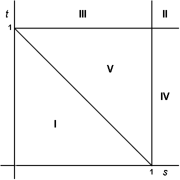
We see that the integration domain T2∩((−∞,s]×(−∞,t])T^{2}\cap((-\infty,s]\times(-\infty,t]) of the inner double integral in (5.1) depends on the position of the point (s,t)(s,t) with respect to the triangle {(u,v) | 0<v<u<1}\left\{\left(u,v\right)\text{ }|\text{ }0<v<u<1\right\}. Clearly T2∩((−∞,s]×(−∞,t])T^{2}\cap((-\infty,s]\times(-\infty,t]) is empty if (s,t)(s,t) is outside the first quadrant, while the first quadrant in the (s,t)(s,t) plane can be split up as the union of five regions with disjoint interiors as in Figure 1 such that the corresponding regions T2∩((−∞,s]×(−∞,t])T^{2}\cap((-\infty,s]\times(-\infty,t]) inside T2T^{2} in the (u,v)(u,v) plane are given by Figure 2.

Refer to caption
Figure 1: The five possible regions of the position of the point (s,t)(s,t).
Refer to caption
Figure 2: The five possibilities of the position of the point (s,t)(s,t) with respect to the u,vu,v axes.

I. The point (s,t)(s,t) lies inside the triangle with 0<s<1,0<t<1−s0<s<1,0<t<1-s. The appropriate part of the integral for WW becomes

I=∫s=01∫t=01−s(∫v=0t∫u=0s(.)dudv)dtdsI=\int_{s=0}^{1}\int_{t=0}^{1-s}\left(\int_{v=0}^{t}\int_{u=0}^{s}(.)\,du\,dv\right)\,dt\,ds

II. The point (s,t)(s,t) lies outside the triangle with 1<s<∞,1<t<∞1<s<\infty,1<t<\infty. The appropriate part of the integral for WW becomes

I=∫s=1∞∫t=1∞(∫v=01∫u=01−v(.)dudv)dtdsI=\int_{s=1}^{\infty}\int_{t=1}^{\infty}\left(\int_{v=0}^{1}\int_{u=0}^{1-v}(.)\,du\,dv\right)\,dt\,ds

III. The point (s,t)(s,t) lies outside the triangle with 0<s<1<t<∞0<s<1<t<\infty. The appropriate part of the integral for WW becomes

I=∫t=1∞∫s=01(∫u=0s∫v=01−u(.)dvdu)dsdtI=\int_{t=1}^{\infty}\int_{s=0}^{1}\left(\int_{u=0}^{s}\int_{v=0}^{1-u}(.)\,dv\,du\right)\,ds\,dt

IV. The point (s,t)(s,t) lies outside the triangle with 0<t<1<s<∞0<t<1<s<\infty. The appropriate part of the integral for WW becomes

I=∫s=1∞∫t=01(∫v=0t∫u=01−v(.)dudv)dtdsI=\int_{s=1}^{\infty}\int_{t=0}^{1}\left(\int_{v=0}^{t}\int_{u=0}^{1-v}(.)\,du\,dv\right)\,dt\,ds

V. The point (s,t)(s,t) lies outside the triangle with 0<s<1, 1−s<t<10<s<1,\ 1-s<t<1. We divide the region of integration in two parts. The appropriate part of the integral for WW becomes

I=∫s=01∫t=1−s1(∫v=01−s∫u=0s(.)dudv)dtds+∫s=01∫t=1−s1(∫v=1−st∫u=01−v(.)dudv)dtdsI=\int_{s=0}^{1}\int_{t=1-s}^{1}\left(\int_{v=0}^{1-s}\int_{u=0}^{s}(.)\,du\,dv\right)\,dt\,ds+\int_{s=0}^{1}\int_{t=1-s}^{1}\left(\int_{v=1-s}^{t}\int_{u=0}^{1-v}(.)\,du\,dv\right)\,dt\,ds

For the fractional derivative we get (the roman numbers refer to the cases in Figure 2)

Wμ,ν\displaystyle W^{\mu,\nu} [f]​(x,y)​[h1​(α,β,γ,k,n)Γ⁡(k−μ)​Γ​(n−k−ν)​1δν+μ]−1=\displaystyle[f](x,y)\left[\dfrac{h_{1}(\alpha,\beta,\gamma,k,n)}{\Gamma(k-\mu)\Gamma(n-k-\nu)}\dfrac{1}{\delta^{\nu+\mu}}\right]^{-1}=
=∫s=01∫t=01−sf(x+δs,y+δt)(∫v=0t∫u=0s (.)dudv)dtds+(I)\displaystyle=\int_{s=0}^{1}\int_{t=0}^{1-s}f(x+\delta s,y+\delta t)\left(\int_{v=0}^{t}\int_{u=0}^{s}\text{ \ }(.)\,du\,dv\right)\,dt\,ds+\qquad\qquad\quad\ \text{(I)}
+∫s=1∞∫t=1∞f(x+δs,y+δt)(∫v=01∫u=01−v(.)dudv)dtds+(II)\displaystyle+\int_{s=1}^{\infty}\int_{t=1}^{\infty}f(x+\delta s,y+\delta t)\left(\int_{v=0}^{1}\int_{u=0}^{1-v}(.)\,du\,dv\right)\,dt\,ds+\qquad\qquad\qquad\ \text{(II)}
+∫t=1∞∫s=01 f(x+δs,y+δt)(∫u=0s∫v=01−u(.)dvdu)dsdt+(III)\displaystyle+\int_{t=1}^{\infty}\int_{s=0}^{1}\text{ }f(x+\delta s,y+\delta t)\left(\int_{u=0}^{s}\int_{v=0}^{1-u}(.)\,dv\,du\right)\,ds\,dt+\qquad\qquad\quad\ \ \text{(III)}
+∫s=1∞∫t=01f(x+δs,y+δt)(∫v=0t∫u=01−v(.)dudv)dtds+ (IV)\displaystyle+\int_{s=1}^{\infty}\int_{t=0}^{1}f(x+\delta s,y+\delta t)\left(\int_{v=0}^{t}\int_{u=0}^{1-v}(.)\,du\,dv\right)\,dt\,ds+\qquad\qquad\qquad\text{ (IV)}
+∫s=01∫t=1−s1f(x+δs,y+δt)(∫v=01−s∫u=0s(.)dudv)dtds+ (V)\displaystyle+\int_{s=0}^{1}\int_{t=1-s}^{1}f(x+\delta s,y+\delta t)\left(\int_{v=0}^{1-s}\int_{u=0}^{s}(.)\,du\,dv\right)\,dt\,ds+\qquad\qquad\quad\ \text{ (V)}
+∫s=01∫t=1−s1f(x+δs,y+δt)(∫v=1−st∫u=01−v(.)dudv)dtds\displaystyle\quad\quad\quad+\int_{s=0}^{1}\int_{t=1-s}^{1}f(x+\delta s,y+\delta t)\left(\int_{v=1-s}^{t}\int_{u=0}^{1-v}(.)\,du\,dv\right)\,dt\,ds

The abbreviation (.)(.) stands for

(.)=(s−u)k−μ−1(t−v)n−k−ν−1Uk,nα,β,γ(u,v)uαvβ(1−u−v)γ(.)=(s-u)^{k-\mu-1}(t-v)^{n-k-\nu-1}U_{k,n}^{\alpha,\beta,\gamma}(u,v)u^{\alpha}v^{\beta}(1-u-v)^{\gamma} (5.4)

For Uk,nα,β,γ​(u,v)U_{k,n}^{\alpha,\beta,\gamma}(u,v) we repeat formulas (2.5) and (2.6):

Uk,nα,β,γ​(u,v)=1uα​vβ​(1−u−v)γ​∂n∂uk​∂vn−k​[uk+α​vn−k+β​(1−u−v)n+γ]U_{k,n}^{\alpha,\beta,\gamma}(u,v)=\dfrac{1}{u^{\alpha}v^{\beta}(1-u-v)^{\gamma}}\\ \dfrac{\partial^{n}}{\partial u^{k}\partial v^{n-k}}\left[u^{k+\alpha}v^{n-k+\beta}(1-u-v)^{n+\gamma}\right] (5.5)
Uk,nα,β,γ​(x,y)=(α+1)k​(β+1)n−k​(1−x−y)−γF2​(−γ−n,α+1+k,β+1+n−k,α+1,β+1,x,y)\qquad\qquad\ U_{k,n}^{\alpha,\beta,\gamma}(x,y)=(\alpha+1)_{k}(\beta+1)_{n-k}(1-x-y)^{-\gamma}\\ F_{2}(-\gamma-n;\alpha+1+k,\beta+1+n-k;\alpha+1,\beta+1;x,y)

for 0≤k≤n0\leq k\leq n. We can use both formulas to compute the fractional derivatives. The results will be of course the same, but with (5.5) there appear some nice results and so we continue with (5.5).

For the integrals inside the brackets in () we can use (5.4) and (5.5) and write in general

∬V(.)dudv==∬V∂k∂uk​∂n−k∂vn−k​[uk+α​vn−k+β​(1−u−v)n+γ]​(s−u)k−μ−1​(t−v)n−k−ν−1​𝑑u​𝑑v\iint_{V}(.)\,du\,dv=\\ =\iint_{V}\dfrac{\partial^{k}}{\partial u^{k}}\dfrac{\partial^{n-k}}{\partial v^{n-k}}\left[u^{k+\alpha}v^{n-k+\beta}(1-u-v)^{n+\gamma}\right](s-u)^{k-\mu-1}(t-v)^{n-k-\nu-1}\,du\,dv

After kk-fold integration by parts with respect to the variable uu we get

∬V(.)dudv[(−1)kΓ⁡(k−μ)Γ⁡(−μ)]−1==∬V(s−u)−μ−1​∂n−k∂vn−k​[uk+α​vn−k+β​(1−u−v)n+γ]​(t−v)n−k−ν−1​𝑑u​𝑑v\iint_{V}(.)\,du\,dv\left[(-1)^{k}\dfrac{\Gamma(k-\mu)}{\Gamma(-\mu)}\right]^{-1}=\\ =\iint\nolimits_{V}(s-u)^{-\mu-1}\dfrac{\partial^{n-k}}{\partial v^{n-k}}\left[u^{k+\alpha}v^{n-k+\beta}(1-u-v)^{n+\gamma}\right](t-v)^{n-k-\nu-1}\,du\,dv

After (n−k)(n-k)-fold integration by parts with respect to the variable vv we get

∬V(.)dudv[(−1)nΓ⁡(k−μ)Γ⁡(−μ)Γ⁡(n−k−ν)Γ⁡(−ν)]−1==∬Vuk+α​(s−u)−μ−1​(1−u−v)n+γ​vn−k+β​(t−v)−ν−1​𝑑u​𝑑v\iint_{V}(.)\,du\,dv\left[(-1)^{n}\dfrac{\Gamma(k-\mu)}{\Gamma(-\mu)}\dfrac{\Gamma(n-k-\nu)}{\Gamma(-\nu)}\right]^{-1}=\\ =\iint\nolimits_{V}u^{k+\alpha}(s-u)^{-\mu-1}(1-u-v)^{n+\gamma}v^{n-k+\beta}(t-v)^{-\nu-1}\,du\,dv

Combination of (5.2) and () gives

Wμ,ν​[f]​(x,y)\displaystyle W^{\mu,\nu}[f](x,y) [1Γ⁡(−μ)​Γ​(−ν)​1B⁡(k+α+1,n+γ+1,n−k+β+1)​1δν+μ]−1=\displaystyle\left[\dfrac{1}{\Gamma(-\mu)\Gamma(-\nu)}\dfrac{1}{B(k+\alpha+1,n+\gamma+1,n-k+\beta+1)}\dfrac{1}{\delta^{\nu+\mu}}\right]^{-1}=
=∫01∫01−sf(x+δs,y+δt)I1(s,t)dtds+ (I)\displaystyle=\int_{0}^{1}\int_{0}^{1-s}f(x+\delta s,y+\delta t)I_{1}(s,t)\,dt\,ds+\qquad\qquad\text{ \ \ \ \ (I)}
+∫1∞∫1∞f(x+δs,y+δt)I3(s,t)dtds+(II)\displaystyle+\int_{1}^{\infty}\int_{1}^{\infty}f(x+\delta s,y+\delta t)I_{3}(s,t)\,dt\,ds+\qquad\qquad\qquad\text{(II)}
+∫1∞∫01 f(x+δs,y+δt)I2(s,t)dsdt+(III)\displaystyle+\int_{1}^{\infty}\int_{0}^{1}\text{ }f(x+\delta s,y+\delta t)I_{2}(s,t)\,ds\,dt+\qquad\qquad\qquad\text{(III)}
+∫1∞∫01 f(x+δs,y+δt)I4(s,t)dtds+(IV)\displaystyle+\int_{1}^{\infty}\int_{0}^{1}\text{ }f(x+\delta s,y+\delta t)I_{4}(s,t)\,dt\,ds+\qquad\qquad\qquad\text{(IV)}
+∫01∫1−s1 f(x+δs,y+δt)I5(s,t)dtds+(V)\displaystyle+\int_{0}^{1}\int_{1-s}^{1}\text{ }f(x+\delta s,y+\delta t)I_{5}(s,t)\,dt\,ds+\qquad\qquad\qquad\text{(V)}
+∫01∫1−s1f(x+δs,y+δt)I6(s,t)dtds\displaystyle\qquad\qquad\qquad+\int_{0}^{1}\int_{1-s}^{1}f(x+\delta s,y+\delta t)I_{6}(s,t)\,dt\,ds

Putting a=k+α+1a=k+\alpha+1, b=n−k+β+1b=n-k+\beta+1, c=−μc=-\mu, d=−νd=-\nu and e=−n−γe=-n-\gamma we get for the functions I1..6​(s,t)I_{1..6}(s,t)

I1​(s,t)=∫0t(∫0sua−1​(s−u)c−1​(1−u−v)−e​𝑑u)​vb−1​(t−v)d−1​𝑑vI_{1}(s,t)=\int_{0}^{t}\left(\int_{0}^{s}u^{a-1}(s-u)^{c-1}(1-u-v)^{-e}du\right)v^{b-1}(t-v)^{d-1}dv (5.6)

with region for ss and tt:0<s<1,0<t<1−s\qquad 0<s<1,0<t<1-s

I2​(s,t)=∫01(∫01−vua−1​(s−u)c−1​(1−u−v)−e​𝑑u)​vb−1​(t−v)d−1​𝑑vI_{2}(s,t)=\int_{0}^{1}\left(\int_{0}^{1-v}u^{a-1}(s-u)^{c-1}(1-u-v)^{-e}du\right)v^{b-1}(t-v)^{d-1}dv (5.7)

with region for ss and tt:1<s<∞,1<t<∞\qquad 1<s<\infty,1<t<\infty

I3​(s,t)=∫0s(∫01−uvb−1​(t−v)d−1​(1−u−v)−e​𝑑v)​ua−1​(s−u)c−1​𝑑uI_{3}(s,t)=\int_{0}^{s}\left(\int_{0}^{1-u}v^{b-1}(t-v)^{d-1}(1-u-v)^{-e}dv\right)u^{a-1}(s-u)^{c-1}du (5.8)

with region for ss and tt:0<s<1<t<∞\qquad 0<s<1<t<\infty

I4​(s,t)=∫0t(∫01−vua−1​(s−u)c−1​(1−u−v)−e​𝑑u)​vb−1​(t−v)d−1​𝑑vI_{4}(s,t)=\int_{0}^{t}\left(\int_{0}^{1-v}u^{a-1}(s-u)^{c-1}(1-u-v)^{-e}du\right)v^{b-1}(t-v)^{d-1}dv (5.9)

with region for ss and tt:0<t<1<s<∞\qquad 0<t<1<s<\infty

I5​(s,t)=∫01−s(∫0sua−1​(s−u)c−1​(1−u−v)−e​𝑑u)​vb−1​(t−v)d−1​𝑑vI_{5}(s,t)=\int_{0}^{1-s}\left(\int_{0}^{s}u^{a-1}(s-u)^{c-1}(1-u-v)^{-e}du\right)v^{b-1}(t-v)^{d-1}dv (5.10)
I6​(s,t)=∫1−st(∫01−vua−1​(s−u)c−1​(1−u−v)−e​𝑑u)​vb−1​(t−v)d−1​𝑑vI_{6}(s,t)=\int_{1-s}^{t}\left(\int_{0}^{1-v}u^{a-1}(s-u)^{c-1}(1-u-v)^{-e}du\right)v^{b-1}(t-v)^{d-1}dv (5.11)

with region for ss and tt:0<s<1, 1−s<t<1\qquad 0<s<1,\ 1-s<t<1

We will treat the evaluation of the integrals I1,…,6I_{1,\dots,6} in the next subsections.

5.1 The integral I1​(s,t)I_{1}(s,t)

For the computation of the integral I1​(s,t)I_{1}(s,t) we write the integral (5.6) as

I1​(s,t)=sa+c−1​tb+d−1​∫01∫01ua−1​vb−1​(1−u)c−1​(1−v)d−1​(1−s​u−t​v)−e​𝑑u​𝑑vI_{1}(s,t)=s^{a+c-1}t^{b+d-1}\int_{0}^{1}\int_{0}^{1}u^{a-1}v^{b-1}(1-u)^{c-1}(1-v)^{d-1}(1-su-tv)^{-e}\,du\,dv (5.12)

The integrals are convergent if 0<Re⁡(a)<Re⁡(a+c)0<\operatorname{Re}(a)<\operatorname{Re}(a+c) and 0<Re⁡(b)<Re⁡(b+d)0<\operatorname{Re}(b)<\operatorname{Re}(b+d). Formula (5.12) is the integral representation for the F2F_{2} Appell function [7, 5.8.1.(2)]. We get

I1​(s,t)=B⁡(a,c)​B​(b,d)​sa+c−1​tb+d−1​F2​(e,a,b,a+c,b+d,s,t)I_{1}(s,t)=B(a,c)B(b,d)s^{a+c-1}t^{b+d-1}F_{2}(e;a,b;a+c,b+d;s,t)

5.2 The integral I2​(s,t)I_{2}(s,t)

For the computation of the integral I2​(s,t)I_{2}(s,t) we write the integral (5.7) as

I2​(s,t)=sc−1​td−1​∫01∫01−vua−1​vb−1​(1−u−v)−e​(1−1s​u)c−1​(1−1t​v)d−1​𝑑u​𝑑vI_{2}(s,t)=s^{c-1}t^{d-1}\int_{0}^{1}\int_{0}^{1-v}u^{a-1}v^{b-1}(1-u-v)^{-e}\left(1-\dfrac{1}{s}u\right)^{c-1}\left(1-\dfrac{1}{t}v\right)^{d-1}\,du\,dv (5.13)

The integrals are convergent if Re⁡(a),Re⁡(b),Re⁡(1−e)>0\operatorname{Re}(a),\operatorname{Re}(b),\operatorname{Re}(1-e)>0. Formula (5.13) is the integral representation for the F3F_{3} Appell function [7, 5.8.1.(3)]. We get

I2​(s,t)=B⁡(a,b,1−e)​sc−1​td−1​F3​(a,b,1−c,1−d,a+b+1−e,1s,1t)I_{2}(s,t)=B(a,b,1-e)s^{c-1}t^{d-1}F_{3}\left(a,b;1-c,1-d;a+b+1-e;\dfrac{1}{s},\dfrac{1}{t}\right) (5.14)

5.3 The integral I3​(s,t)I_{3}(s,t)

For the computation of the integral I3​(s,t)I_{3}(s,t) we write the integral (5.8) as

I3​(s,t)=sa+c−1​td−1∫01∫01ua−1​vb−1​(1−u)c−1​(1−v)−e​(1−s​u)b−e​(1−1t​v+st​u​v)d−1​𝑑u​𝑑vI_{3}(s,t)=s^{a+c-1}t^{d-1}\\ \int_{0}^{1}\int_{0}^{1}u^{a-1}v^{b-1}(1-u)^{c-1}(1-v)^{-e}(1-su)^{b-e}\left(1-\dfrac{1}{t}v+\dfrac{s}{t}uv\right)^{d-1}\,du\,dv (5.15)

Formula (5.15) is an integral representation of the H2H_{2} function [5, (3.4)]. We get

I3​(s,t)=B⁡(a,c)​B​(b,1−e)​sa+c−1​td−1​H2​(e−b,a,1−d,b,a+c,s,−1t)I_{3}(s,t)=B(a,c)B(b,1-e)s^{a+c-1}t^{d-1}H_{2}\left(e-b,a,1-d,b;a+c;s,-\dfrac{1}{t}\right) (5.16)

5.4 The integral I4​(s,t)I_{4}(s,t)

For I4​(s,t)I_{4}(s,t) we look at I2​(s,t)I_{2}(s,t). Interchanging in I2​(s,t)I_{2}(s,t) the parameters aa and bb, cc and dd and the variables ss and tt we get I4​(s,t)I_{4}(s,t). So from (5.16) we get directly

I4​(s,t)=B⁡(a,1−e)​B​(b,d)​tb+d−1​sc−1​H2​(e−a,b,1−c,a,b+d,t,−1s)I_{4}(s,t)=B(a,1-e)B(b,d)t^{b+d-1}s^{c-1}H_{2}\left(e-a,b,1-c,a;b+d;t,-\dfrac{1}{s}\right)

5.5 The integral I5​(s,t)I_{5}(s,t)

For I5​(s,t)I_{5}(s,t) we write the inner integral of (5.10) as

∫0sua−1​(s−u)c−1​(1−v−u)−e​𝑑u=B⁡(a,c)​sa+c−1​(1−v)−e​2​F1​(a,ea+c,s1−v)\int_{0}^{s}u^{a-1}(s-u)^{c-1}(1-v-u)^{-e}du=B(a,c)s^{a+c-1}(1-v)^{-e}\,\mbox{}_{2}F_{1}\!\left(\genfrac{}{}{0.0pt}{}{a,e}{a+c};\dfrac{s}{1-v}\right)

with convergence conditions Re⁡(a),Re⁡(c),Re⁡(c−e)>0\operatorname{Re}(a),\operatorname{Re}(c),\operatorname{Re}(c-e)>0 and s1−v≤1\dfrac{s}{1-v}\leq 1. Substitution in (5.10) and replacing vv by (1−s)​v(1-s)v gives

I5​(s,t)=B⁡(a,c)​sa+c−1​td−1​(1−s)b×∫01vb−1​(1−(1−s)​v)−e​(1−1−st​v)d−1​2​F1​(a,ea+c,s1−(1−s)​v)​𝑑vI_{5}(s,t)=B(a,c)s^{a+c-1}t^{d-1}(1-s)^{b}\\ \times\int_{0}^{1}v^{b-1}\big(1-(1-s)v\big)^{-e}\left(1-\dfrac{1-s}{t}v\right)^{d-1}\,\mbox{}_{2}F_{1}\!\left(\genfrac{}{}{0.0pt}{}{a,e}{a+c};\dfrac{s}{1-(1-s)v}\right)dv (5.17)

Because the computation of the integral is very long we only give the result from [4, section 6.5.5.]

I5​(s,t)\displaystyle I_{5}(s,t) =B⁡(c,e−c)​B​(b,c−e+1)​sa−1​td−1​(1−s)b+c−e\displaystyle=B(c,e-c)B(b,c-e+1)s^{a-1}t^{d-1}(1-s)^{b+c-e}
×F3​(1−a,b;c,1−db+c−e+1,s−1s,1−st)+\displaystyle\qquad\qquad\qquad\qquad\qquad\qquad\times F_{3}\left(\begin{array}[]{c}1-a,b;c,1-d\\ b+c-e+1\end{array};\dfrac{s-1}{s},\dfrac{1-s}{t}\right)+
+B⁡(a,c−e)​B​(b,d)​sa+c−1​tb+d−1​FP​(e,b,a,b+d,a+c,t,s)−\displaystyle+B(a,c-e)B(b,d)s^{a+c-1}t^{b+d-1}F_{P}(e,b,a,b+d,a+c;t,s)-
−B⁡(a,c−e)d​sa+c−e−1​tb−1​(s+t−1)d\displaystyle-\dfrac{B(a,c-e)}{d}s^{a+c-e-1}t^{b-1}(s+t-1)^{d}
×F3~​(1,1−b;e−a−c+1,dd+1,ee−c+1,s+t−1s,s+t−1t)\displaystyle\qquad\times\widetilde{F_{3}}\left(\begin{array}[]{c}1,1-b;e-a-c+1,d\\ d+1\end{array};\begin{array}[]{c}e\\ e-c+1\end{array};\dfrac{s+t-1}{s},\dfrac{s+t-1}{t}\right)

with convergence conditions for the FPF_{P} function: |t|<1\left|t\right|<1, |s−1|<1\left|s-1\right|<1. The convergence conditions of the F3F_{3} function are: |s−1s|<1\left|\dfrac{s-1}{s}\right|<1 and |1−st|<1\left|\dfrac{1-s}{t}\right|<1. This gives a region of convergence 12<s<1\dfrac{1}{2}<s<1. But after analytical continuation (see (B.1)) this function is well-defined for s−1s<1\dfrac{s-1}{s}<1 and 1−st<1\dfrac{1-s}{t}<1. For the extended F3F_{3} function we have with analytical continuation convergence for the same region as for the F3F_{3} function (see appendix B.2).This includes the (s,t)(s,t) domain on which the integral I5​(s,t)I_{5}(s,t) is defined. For the parameters we have the convergence conditions: 0<Re⁡(a),Re⁡(b),Re⁡(c),Re⁡(d),Re⁡(e)<Re⁡(c)+10<\operatorname{Re}(a),\operatorname{Re}(b),\operatorname{Re}(c),\operatorname{Re}(d),\operatorname{Re}(e)<\operatorname{Re}(c)+1.

5.6 The integral I6​(s,t)I_{6}(s,t)

For I6​(s,t)I_{6}(s,t) we write the inner integral of (5.11) as

∫01−vua−1​(s−u)c−1​(1−v−u)−e​𝑑u=B⁡(a,1−e)​sc−1​(1−v)a−e​2​F1​(a,1−ca−e+1,1−vs)\int_{0}^{1-v}u^{a-1}(s-u)^{c-1}(1-v-u)^{-e}du=B(a,1-e)s^{c-1}(1-v)^{a-e}\,\mbox{}_{2}F_{1}\!\left(\genfrac{}{}{0.0pt}{}{a,1-c}{a-e+1};\dfrac{1-v}{s}\right)

with convergence conditions Re⁡(a),Re⁡(1−e)>0\operatorname{Re}(a),\operatorname{Re}(1-e)>0 and 1−vs<1\dfrac{1-v}{s}<1.

Because the computation of the integral is also very long we only give the result from [4, section 6.5.6.]

I6​(s,t)\displaystyle I_{6}(s,t) =B⁡(a,c−e)d​sa+c−e−1​tb−1​(s+t−1)d\displaystyle=\dfrac{B(a,c-e)}{d}s^{a+c-e-1}t^{b-1}(s+t-1)^{d}
×F3~​(1,1−b;e−a−c+1,dd+1,ee−c+1,s+t−1s,s+t−1t)+\displaystyle\qquad\qquad\times\widetilde{F_{3}}\left(\begin{array}[]{c}1,1-b;e-a-c+1,d\\ d+1\end{array};\begin{array}[]{c}e\\ e-c+1\end{array};\dfrac{s+t-1}{s},\dfrac{s+t-1}{t}\right)+
+B⁡(1−e,e−c)​B​(d,1−e+c)​sa−1​tb−1​(s+t−1)c+d−e\displaystyle+B(1-e,e-c)B(d,1-e+c)s^{a-1}t^{b-1}(s+t-1)^{c+d-e}
×F3​(1−a,1−b;c,dc+d−e+1,s+t−1s,s+t−1t)\displaystyle\qquad\qquad\times F_{3}\left(\begin{array}[]{c}1-a,1-b;c,d\\ c+d-e+1\end{array};\dfrac{s+t-1}{s},\dfrac{s+t-1}{t}\right)

with convergence conditions: Re⁡(a),Re⁡(d),Re⁡(1−e),Re⁡(c−e+1)>0\operatorname{Re}(a),\operatorname{Re}(d),\operatorname{Re}(1-e),\operatorname{Re}(c-e+1)>0.

5.7 The summation of the integrals I5​(s,t)I_{5}(s,t) and I6​(s,t)I_{6}(s,t)

When adding the functions I5​(s,t)I_{5}(s,t) (5.5) and I6​(s,t)I_{6}(s,t) (5.6) the extended F3F_{3} functions will be eliminated. We get

I5​(s,t)+I6​(s,t)\displaystyle I_{5}(s,t)+I_{6}(s,t) =B⁡(a,c−e)​B​(b,d)​sa+c−1​tb+d−1​FP​(e,b,a,b+d,a+c,t,s)+\displaystyle=B(a,c-e)B(b,d)s^{a+c-1}t^{b+d-1}F_{P}(e,b,a,b+d,a+c;t,s)+
+B⁡(c,e−c)​B​(b,c−e+1)​sa−1​(1−s)b+c−e​td−1\displaystyle+B(c,e-c)B(b,c-e+1)s^{a-1}(1-s)^{b+c-e}t^{d-1}
F3​(1−a,b;c,1−db+c−e+1,s−1s,1−st)+\displaystyle\qquad\qquad\qquad\qquad\qquad F_{3}\left(\begin{array}[]{c}1-a,b;c,1-d\\ b+c-e+1\end{array};\dfrac{s-1}{s},\dfrac{1-s}{t}\right)+
+B⁡(1−e,e−c)​B​(d,1−e+c)​sa−1​tb−1​(s+t−1)c+d−e\displaystyle+B(1-e,e-c)B(d,1-e+c)s^{a-1}t^{b-1}(s+t-1)^{c+d-e}
F3​(1−a,1−b;c,dc+d−e+1,s+t−1s,s+t−1t)\displaystyle\qquad\qquad\qquad\qquad F_{3}\left(\begin{array}[]{c}1-a,1-b;c,d\\ c+d-e+1\end{array};\dfrac{s+t-1}{s},\dfrac{s+t-1}{t}\right)

The power series of the functions FPF_{P} (B.7) and F3F_{3} (B.1) are convergent in the region 0<s<1,1−s<t<10<s<1,1-s<t<1. For the first F3F_{3} function we use the analytical continuation over the whole (s,t)(s,t) region. For the parameters we get the convergence conditions: 0<Re⁡(a),Re⁡(b),Re⁡(c),Re⁡(d)0<~\operatorname{Re}(a),\operatorname{Re}(b),\operatorname{Re}(c),\operatorname{Re}(d) and Re⁡(e)<1\operatorname{Re}(e)<1. From [13, p 441] we get

F3​(a0,b1;b2,c1c2,x1,x2)\displaystyle F_{3}\left(\begin{array}[]{c}a_{0},b_{1};b_{2},c_{1}\\ c_{2}\end{array};x_{1},x_{2}\right) =Γ⁡(c2)​Γ​(c2−b1−c1)Γ⁡(c2−b1)​Γ​(c2−c1)​(x1)−a0​(x2)−b1\displaystyle=\dfrac{\Gamma(c_{2})\Gamma(c_{2}-b_{1}-c_{1})}{\Gamma(c_{2}-b_{1})\Gamma(c_{2}-c_{1})}(x_{1})^{-a_{0}}(x_{2})^{-b_{1}}
FQ​(b2+c1−c2+1,b2,c1,1−a0+b2,c1−b1+1,1x1,1x2)+\displaystyle F_{Q}\left(b_{2}+c_{1}-c_{2}+1,b_{2},c_{1};1-a_{0}+b_{2},c_{1}-b_{1}+1;\dfrac{1}{x_{1}},\dfrac{1}{x_{2}}\right)+
+Γ⁡(c2)​Γ​(b1+c1−c2)Γ⁡(b1)​Γ​(c1)​(x2)1−c2​(1−x2)c2−b1−c1\displaystyle+\dfrac{\Gamma(c_{2})\Gamma(b_{1}+c_{1}-c_{2})}{\Gamma(b_{1})\Gamma(c_{1})}(x_{2})^{1-c_{2}}(1-x_{2})^{c_{2}-b_{1}-c_{1}}
F3​(a0,1−b1;b2,1−c11−b1−c1+c2,x1​(x2−1)x2,1−x2)\displaystyle\qquad\quad F_{3}\left(\begin{array}[]{c}a_{0},1-b_{1};b_{2},1-c_{1}\\ 1-b_{1}-c_{1}+c_{2}\end{array};\dfrac{x_{1}(x_{2}-1)}{x_{2}},1-x_{2}\right)

After application of (5.7) to the second F3F_{3} function of (5.7) we get

I5​(s,t)+I6​(s,t)\displaystyle I_{5}(s,t)+I_{6}(s,t) =B⁡(a,c−e)​B​(b,d)​sa+c−1​tb+d−1​FP​(e,b,a,b+d,a+c,t,s)+\displaystyle=B(a,c-e)B(b,d)s^{a+c-1}t^{b+d-1}F_{P}(e,b,a,b+d,a+c;t,s)+
+B⁡(1−e,e−c)​B​(d,c−e+b)​(s+t−1)a+b+c+d−e−2\displaystyle+B(1-e,e-c)B(d,c-e+b)(s+t-1)^{a+b+c+d-e-2}
FQ​(e,c,d,a+c,b+d,ss+t−1,ts+t−1)+\displaystyle\qquad\qquad\qquad\qquad\qquad\qquad F_{Q}\left(e,c,d;a+c,b+d;\dfrac{s}{s+t-1},\dfrac{t}{s+t-1}\right)+
+Γ⁡(e−c)​Γ​(c−e+1)​[Γ⁡(b)​Γ​(c)Γ⁡(e)​Γ​(c+b−e+1)+Γ⁡(1−e)​Γ​(e−b−c)Γ⁡(1−c)​Γ​(1−b)]\displaystyle+\Gamma(e-c)\Gamma(c-e+1)\left[\dfrac{\Gamma(b)\Gamma(c)}{\Gamma(e)\Gamma(c+b-e+1)}+\dfrac{\Gamma(1-e)\Gamma(e-b-c)}{\Gamma(1-c)\Gamma(1-b)}\right]
sa−1​(1−s)b+c−e​td−1​F3​(1−a,b;c,1−db+c−e+1,s−1s,1−st)\displaystyle\qquad\qquad\qquad\qquad s^{a-1}(1-s)^{b+c-e}t^{d-1}F_{3}\left(\begin{array}[]{c}1-a,b;c,1-d\\ b+c-e+1\end{array};\dfrac{s-1}{s},\dfrac{1-s}{t}\right)

The function FQF_{Q} is defined in (B.8). After some simplification of the terms within the square brackets we get

I5​(s,t)+I6​(s,t)\displaystyle I_{5}(s,t)+I_{6}(s,t) =B⁡(a,c−e)​B​(b,d)​sa+c−1​tb+d−1​FP​(e,b,a,b+d,a+c,t,s)+\displaystyle=B(a,c-e)B(b,d)s^{a+c-1}t^{b+d-1}F_{P}(e,b,a,b+d,a+c;t,s)+
+B⁡(1−e,e−c)​B​(d,c−e+b)​sa+c−1​tb+d−1​(s+t−1)−e\displaystyle+B(1-e,e-c)B(d,c-e+b)s^{a+c-1}t^{b+d-1}(s+t-1)^{-e}
FQ​(e,c,d,a+c,b+d,ss+t−1,ts+t−1)+\displaystyle\qquad\qquad\qquad\qquad\qquad\qquad F_{Q}\left(e,c,d;a+c,b+d;\dfrac{s}{s+t-1},\dfrac{t}{s+t-1}\right)+
+B⁡(e−b−c,c)​B​(1−e,b)​sa−1​(1−s)b+c−e​td−1\displaystyle+B(e-b-c,c)B(1-e,b)s^{a-1}\left(1-s\right)^{b+c-e}t^{d-1}
F3​(1−a,b;c,1−db+c−e+1,s−1s,1−st)\displaystyle\qquad\qquad\qquad\qquad\qquad\qquad\qquad\qquad F_{3}\left(\begin{array}[]{c}1-a,b;c,1-d\\ b+c-e+1\end{array};\dfrac{s-1}{s},\dfrac{1-s}{t}\right)

The power series of the FPF_{P} and the FQF_{Q} functions are convergent in the region {0<s<1∧1−s<t<1}\{0<s<1\wedge 1-s<t<1\}. For the F3F_{3} function we use an analytical continuation so we get the convergence in the right region. For the parameters we get the convergence conditions: 0<Re⁡(a,b,c,d,e)<10<\operatorname{Re}(a,b,c,d,e)<1.

5.8 Summary of the integrals I1..6​(s,t)I_{1..6}(s,t)

We give a summary of the functions I1..9​(s,t)I_{1..9}(s,t)

I1​(s,t)=B⁡(a,c)​B​(b,d)​sa+c−1​tb+d−1​F2​(e,a,b,a+c,b+d,s,t)I_{1}(s,t)=B(a,c)B(b,d)s^{a+c-1}t^{b+d-1}F_{2}(e;a,b;a+c,b+d;s,t) (5.38)

with 0<s<1,0<t<1−s0<s<1,0<t<1-s and 0<Re⁡(a)<Re⁡(a+c)0<\operatorname{Re}(a)<\operatorname{Re}(a+c), 0<Re⁡(b)<Re⁡(b+d)0<\operatorname{Re}(b)<\operatorname{Re}(b+d).

I2​(s,t)=B⁡(a,b,1−e)​sc−1​td−1​F3​(a,b,1−c,1−d,a+b+1−e,1s,1t)I_{2}(s,t)=B(a,b,1-e)s^{c-1}t^{d-1}F_{3}\left(a,b;1-c,1-d;a+b+1-e;\dfrac{1}{s},\dfrac{1}{t}\right)

with 1<s<∞,1<t<∞1<s<\infty,1<t<\infty and Re⁡(a),Re⁡(b),Re⁡(1−e)>0\operatorname{Re}(a),\operatorname{Re}(b),\operatorname{Re}(1-e)>0.

I3​(s,t)=B⁡(a,c)​B​(b,1−e)​sa+c−1​td−1​H2​(e−b,a,1−d,b,a+c,s,−1t)I_{3}(s,t)=B(a,c)B(b,1-e)s^{a+c-1}t^{d-1}H_{2}\left(e-b,a,1-d,b;a+c;s,-\dfrac{1}{t}\right) (5.39)

with 0<s<1<t<∞0<s<1<t<\infty and Re⁡(a),Re⁡(b)>0,Re⁡(c)>0\operatorname{Re}(a),\operatorname{Re}(b)>0,\operatorname{Re}(c)>0.

I4​(s,t)=B⁡(a,1−e)​B​(b,d)​tb+d−1​sc−1​H2​(e−a,b,1−c,a,b+d,t,−1s)I_{4}(s,t)=B(a,1-e)B(b,d)t^{b+d-1}s^{c-1}H_{2}\left(e-a,b,1-c,a;b+d;t,-\dfrac{1}{s}\right) (5.40)

with 0<t<1<s<∞0<t<1<s<\infty and Re⁡(a),Re⁡(b),Re⁡(d)>0\operatorname{Re}(a),\operatorname{Re}(b),\operatorname{Re}(d)>0.

I5​(s,t)+I6​(s,t)\displaystyle I_{5}(s,t)+I_{6}(s,t) =B⁡(a,c−e)​B​(b,d)​sa+c−1​tb+d−1​FP​(e,b,a,b+d,a+c,t,s)+\displaystyle=B(a,c-e)B(b,d)s^{a+c-1}t^{b+d-1}F_{P}(e,b,a,b+d,a+c;t,s)+
+B⁡(c,e−c)​B​(b,c−e+1)​sa−1​(1−s)b+c−e​td−1\displaystyle+B(c,e-c)B(b,c-e+1)s^{a-1}(1-s)^{b+c-e}t^{d-1}
F3​(1−a,b;c,1−dc+b−e+1,s−1s,1−st)+\displaystyle\qquad\qquad\qquad\qquad\qquad F_{3}\left(\begin{array}[]{c}1-a,b;c,1-d\\ c+b-e+1\end{array};\dfrac{s-1}{s},\dfrac{1-s}{t}\right)+
+B⁡(1−e,e−c)​B​(d,1−e+c)​tb−1​sa−1​(s+t−1)c+d−e\displaystyle+B(1-e,e-c)B(d,1-e+c)t^{b-1}s^{a-1}(s+t-1)^{c+d-e}
F3​(1−a,1−b;c,dc+d−e+1,s+t−1s,s+t−1t)\displaystyle\qquad\qquad\qquad\qquad F_{3}\left(\begin{array}[]{c}1-a,1-b;c,d\\ c+d-e+1\end{array};\dfrac{s+t-1}{s},\dfrac{s+t-1}{t}\right)

with 0<s<1, 1−s<t<10<s<1,\ 1-s<t<1 and 0<Re⁡(a),Re⁡(c),Re⁡(d),Re⁡(e)<10<\operatorname{Re}(a),\operatorname{Re}(c),\operatorname{Re}(d),\operatorname{Re}(e)<1.
The functions F2F_{2}, F3F_{3}, H2H_{2} and FPF_{P} are all five-parametric double-hypergeometric functions which are solutions of a system of two partial differential equations of second order [14]. This system is associated with the Appell function F2​(a,b1,b2,c1,c2,x,y)F_{2}(a,b_{1},b_{2},c_{1},c_{2};x,y) [7, 5.9(10)]. Note that the orthogonal polynomials (2.6) and (2.8) used for the fractional orthogonal derivative are also expressed in terms of F2F_{2} functions.

5.9 Remarks

Remark 5.1.

It is well-known [7, 5.9(10)] that the F2​(a0,b1,b2,c1,c2,x,y)F_{2}(a_{0};b_{1},b_{2};c_{1},c_{2};x,y) function is a solution of the following system of partial differential equations

x⁡(1−x)​r−x​y​s+[c1−(a0+b1+1)​x]​p−b1​y​q−a0​b1​F2​(x,y)=0x(1-x)r-xys+\Big[c_{1}-(a_{0}+b_{1}+1)x\Big]p-b_{1}yq-a_{0}b_{1}F_{2}(x,y)=0 (5.45)
y⁡(1−y)​t−x​y​s+[c2−(a0+b2+1)​y]​q−b2​x​p−a0​b2​F2​(x,y)=0y(1-y)t-xys+\Big[c_{2}-(a_{0}+b_{2}+1)y\Big]q-b_{2}xp-a_{0}b_{2}F_{2}(x,y)=0 (5.46)

with

p=∂F2​(x,y)∂xq=∂F2​(x,y)∂yr=∂2F2​(x,y)∂x2s=∂2F2​(x,y)∂x​∂yt=∂2F2​(x,y)∂y2p=\dfrac{\partial F_{2}(x,y)}{\partial x}\ \ \ q=\dfrac{\partial F_{2}(x,y)}{\partial y}\ \ \ r=\dfrac{\partial^{2}F_{2}(x,y)}{\partial x^{2}}\ \ \ s=\dfrac{\partial^{2}F_{2}(x,y)}{\partial x\partial y}\ \ \ t=\dfrac{\partial^{2}F_{2}(x,y)}{\partial y^{2}}

Olsson treats all 36 explicit solutions of (5.45) and (5.46) [14]. Using the substitutions a0=e−a−b−c−d+2,b1=1−c,b2=1−d,c1=2−a−c,c2=2−b−da_{0}=e-a-b-c-d+2,\ b_{1}=1-c,\ b_{2}=1-d,\ c_{1}=2-a-c,\ c_{2}=2-b-d and x→s,y→tx\rightarrow s,\ y\rightarrow t he gives among others the following solutions of (5.45) and (5.46)

sa+c−1​tb+d−1​F2​(e;a,ba+c,b+d,s,t)s^{a+c-1}t^{b+d-1}F_{2}\left(\begin{array}[]{c}e;a,b\\ a+c,b+d\end{array};s,t\right) (5.47)
sa+c−1​F2​(e−b−d+1;a,1−da+c,2−b−d,s,t)s^{a+c-1}F_{2}\left(\begin{array}[]{c}e-b-d+1;a,1-d\\ a+c,2-b-d\end{array};s,t\right) (5.48)
sc−1​td−1​F3​(a,b;1−c,1−da+b+1−e,1s,1t)s^{c-1}t^{d-1}F_{3}\left(\begin{array}[]{c}a,b;1-c,1-d\\ a+b+1-e\end{array};\dfrac{1}{s},\dfrac{1}{t}\right) (5.49)
tb+d−1​FP​(e−c−a+1,b,1−c,b+d,2−a−c,t,s)t^{b+d-1}F_{P}(e-c-a+1,b,1-c,b+d,2-a-c;t,s) (5.50)
sa−1​td−1​(1−s)b+c−e​F3​(1−a,b;c,1−db+c−e+1,s−1s,1−st)s^{a-1}t^{d-1}(1-s)^{b+c-e}F_{3}\left(\begin{array}[]{c}1-a,b;c,1-d\\ b+c-e+1\end{array};\dfrac{s-1}{s},\dfrac{1-s}{t}\right) (5.51)
sa−1​tb−1​(1−s−t)c+d−e​F3​(1−a,1−b;c,dc+d−e+1,s+t−1s,s+t−1t)s^{a-1}t^{b-1}(1-s-t)^{c+d-e}F_{3}\left(\begin{array}[]{c}1-a,1-b;c,d\\ c+d-e+1\end{array};\dfrac{s+t-1}{s},\dfrac{s+t-1}{t}\right) (5.52)
sa+c−1​td−1​H2​(e−b,a,1−d,b,a+c,s,−1t)s^{a+c-1}t^{d-1}H_{2}\left(e-b,a,1-d,b;a+c;s,-\dfrac{1}{t}\right) (5.53)

For the integral I1​(s,t)I_{1}(s,t) we see that the function sa+c−1​tb+d−1​F2​(e;a,ba+c,b+d,s,t)s^{a+c-1}t^{b+d-1}F_{2}\left(\begin{array}[]{c}e;a,b\\ a+c,b+d\end{array};s,t\right) equals the solution (5.47).

For the integral I2​(s,t)I_{2}(s,t) we see that the function sc−1​td−1​F3​(a,b,1−c,1−d,a+b+1−e,1s,1t)s^{c-1}t^{d-1}F_{3}\left(a,b;1-c,1-d;a+b+1-e;\dfrac{1}{s},\dfrac{1}{t}\right) equals the solution (5.49).

For the integral I3​(s,t)I_{3}(s,t) we see that the function sa+c−1​td−1​H2​(e−b,a,1−d,b,a+c,s,−1t)s^{a+c-1}t^{d-1}H_{2}\left(e-b,a,1-d,b;a+c;s,-\dfrac{1}{t}\right) equals the solution (5.53).

To compute I4​(s,t)I_{4}(s,t) we can interchange in I3​(s,t)I_{3}(s,t) the parameters aa and bb, cc and dd and the variables ss and tt. Then we see that (5.40) is a solution of (5.45) and (5.46).

For the integral I5​(s,t)+I6​(s,t)I_{5}(s,t)+I_{6}(s,t) we have the functions

L1​(s,t)=sa+c−1​tb+d−1​FP​(e,b,a,b+d,a+c,t,s)L_{1}(s,t)=s^{a+c-1}t^{b+d-1}F_{P}(e,b,a,b+d,a+c;t,s) (5.54)
L2​(s,t)=sa−1​(1−s)b+c−e​td−1​F3​(1−a,b;c,1−db+c−e+1,s−1s,1−st)L_{2}(s,t)=s^{a-1}(1-s)^{b+c-e}t^{d-1}F_{3}\left(\begin{array}[]{c}1-a,b;c,1-d\\ b+c-e+1\end{array};\dfrac{s-1}{s},\dfrac{1-s}{t}\right)
L3​(s,t)=sa−1​tb−1​(s+t−1)c+d−e​F3​(1−a,1−b;c,dc+d−e+1,s+t−1s,s+t−1t)L_{3}\left(s,t\right)=s^{a-1}t^{b-1}(s+t-1)^{c+d-e}F_{3}\left(\begin{array}[]{c}1-a,1-b;c,d\\ c+d-e+1\end{array};\dfrac{s+t-1}{s},\dfrac{s+t-1}{t}\right)

For the function L1​(s,t)L_{1}(s,t) we use the solution [14, (26)] and interchange b1⟷b2,c1⟷c2b_{1}\longleftrightarrow b_{2},c_{1}\longleftrightarrow c_{2} and x1⟷x2x_{1}\longleftrightarrow x_{2}. Then the solution becomes

(x2)1−c2​FP​(a0−c2+1,b1,b2​c2+1,c1,2−c2,x2,x1)\left(x_{2}\right)^{1-c_{2}}F_{P}(a_{0}-c_{2}+1,b_{1},b_{2}c_{2}+1,c_{1},2-c_{2};x_{2},x_{1})

Application to (5.54) gives as result

tb+d−1​FP​(e−c−a+1,b,1−c,b+d,2−a−c,t,s)t^{b+d-1}F_{P}(e-c-a+1,b,1-c,b+d,2-a-c;t,s)

This function is equal (5.50). So L1​(s,t)L_{1}(s,t) is a solution of (5.47) and (5.48).

The function L2​(s,t)L_{2}(s,t) equals the solution (5.51).

The function L3​(s,t)L_{3}(s,t) equals the solution (5.52).

Remark 5.2.

It is clear that the inner double integrals in () are in fact double integrals transformations which transform the solutions of the F2F_{2} equations (5.45) and (5.46) into a solution of the F2F_{2} equations with other parameters.

Remark 5.3.

When looking at Figure 2 case Va we can consider the integral when the arguments are on the boundaries. Then we distinguish four possibilities.

I.  s=1s=1.

For s=1s=1 it can be shown that I5​(1,t)+I6​(1,t)=I4​(1,t)I_{5}(1,t)+I_{6}(1,t)=I_{4}(1,t).
II.  t=1t=1.

For t=1t=1 it can be shown that I5​(s,1)+I6​(s,1)=I3​(s,1)I_{5}(s,1)+I_{6}(s,1)=I_{3}(s,1).
III.  s=t=1s=t=1.

From (5.17) it follows I5​(1,t)=0I_{5}(1,t)=0 and I6​(1,t)=I4​(1,t)I_{6}(1,t)=I_{4}(1,t). For s=t=1s=t=1 it can be shown that I6​(1,1)=I2​(1,1)=I3​(1,1)I_{6}(1,1)=I_{2}(1,1)=I_{3}(1,1).
IV.  s+t=1s+t=1.

For s+t=1s+t=1 it can be shown that I5​(s,1−s)+I6​(s,1−s)=I1​(s,1−s)I_{5}(s,1-s)+I_{6}(s,1-s)=I_{1}(s,1-s).

Remark 5.4.

When looking at case V in Figure 2 we see directly that when interchanging a↔ba\leftrightarrow b, c↔dc\leftrightarrow d, s↔ts\leftrightarrow t and the integration variables u↔vu\leftrightarrow v we get

I5​(a,b,c,d,e,s,t)+I6​(a,b,c,d,e,s,t)=I5​(b,a,d,c,e,t,s)+I6​(b,a,d,c,e,t,s)I_{5}(a,b,c,d,e;s,t)+I_{6}(a,b,c,d,e;s,t)=I_{5}(b,a,d,c;e;t,s)+I_{6}(b,a,d,c;e;t,s) (5.55)

From the symmetry there follows that I5​(s,t)+I6​(s,t)I_{5}(s,t)+I_{6}(s,t) can be written as half the sum of the two sides of (5.55).

Looking at equation (5.8) we see that only the second F3F_{3} function in the right-hand side is symmetrical in the parameters and the arguments. Now write (5.55) as

I5​(a,b,c,d,e,s,t)+I6​(a,b,c,d,e,s,t)\displaystyle I_{5}(a,b,c,d,e;s,t)+I_{6}(a,b,c,d,e;s,t) =λ⁡(I5​(a,b,c,d,e,s,t)+I6​(a,b,c,d,e,s,t))+\displaystyle=\lambda\big(I_{5}(a,b,c,d,e;s,t)+I_{6}(a,b,c,d,e;s,t)\big)+
+(1−λ)​(I5​(b,a,d,c,e,t,s)+I6​(b,a,d,c,e,t,s))\displaystyle+(1-\lambda)\big(I_{5}(b,a,d,c;e;t,s)+I_{6}(b,a,d,c;e;t,s)\big)

Now we can choose λ\lambda so that the second F3F_{3} functions will be eliminated. There results

I5​(s,t)+I6​(s,t)\displaystyle I_{5}(s,t)+I_{6}(s,t) =A1​sa+c−1​tb+d−1​FP​(e,b,a,b+d,a+c,t,s)+\displaystyle=A_{1}\;s^{a+c-1}t^{b+d-1}F_{P}(e,b,a,b+d,a+c;t,s)+
+A2​sa+c−1​tb+d−1​FP​(e,a,b,a+c,b+d,s,t)+\displaystyle+A_{2}\;s^{a+c-1}t^{b+d-1}F_{P}(e,a,b,a+c,b+d;s,t)+
+A3​tb−1​(1−t)a+d−e​sc−1​F3​(d,a;1−b,1−ca+d−e+1,t−1t,1−ts)+\displaystyle+A_{3}\;t^{b-1}(1-t)^{a+d-e}s^{c-1}F_{3}\left(\begin{array}[]{c}d,a;1-b,1-c\\ a+d-e+1\end{array};\dfrac{t-1}{t},\dfrac{1-t}{s}\right)+
+A4​sa−1​(1−s)b+c−e​td−1​F3​(c,b;1−a,1−db+c−e+1,s−1s,1−st)\displaystyle+A_{4}\;s^{a-1}(1-s)^{b+c-e}t^{d-1}F_{3}\left(\begin{array}[]{c}c,b;1-a,1-d\\ b+c-e+1\end{array};\dfrac{s-1}{s},\dfrac{1-s}{t}\right)

with

A1=Γ⁡(a)​Γ​(b)​Γ​(e)​Γ​(c−d)​Γ​(d−c+1)​Γ​(1−e)Γ⁡(a+c−e)​Γ​(b+d)​Γ​(1−d)​Γ​(e−c+1)A_{1}=\dfrac{\Gamma(a)\Gamma(b)\Gamma(e)\Gamma(c-d)\Gamma(d-c+1)\Gamma(1-e)}{\Gamma(a+c-e)\Gamma(b+d)\Gamma(1-d)\Gamma(e-c+1)}
A2=Γ⁡(a)​Γ​(b)​Γ​(e)​Γ​(d−c)​Γ​(c−d+1)​Γ​(1−e)Γ⁡(b+d−e)​Γ​(a+c)​Γ​(1−c)​Γ​(e−d+1)A_{2}=\dfrac{\Gamma(a)\Gamma(b)\Gamma(e)\Gamma(d-c)\Gamma(c-d+1)\Gamma(1-e)}{\Gamma(b+d-e)\Gamma(a+c)\Gamma(1-c)\Gamma(e-d+1)}
A3=Γ⁡(a)​Γ​(d)​Γ​(c−d)​Γ​(d−c+1)​Γ​(1−e)Γ⁡(c)​Γ​(1−c)​Γ​(a+d−e+1)A_{3}=\dfrac{\Gamma(a)\Gamma(d)\Gamma(c-d)\Gamma(d-c+1)\Gamma(1-e)}{\Gamma(c)\Gamma(1-c)\Gamma(a+d-e+1)}\qquad
A4=Γ⁡(b)​Γ​(c)​Γ​(d−c)​Γ​(c−d+1)​Γ​(1−e)Γ⁡(d)​Γ​(1−d)​Γ​(c+b−e+1)A_{4}=\dfrac{\Gamma(b)\Gamma(c)\Gamma(d-c)\Gamma(c-d+1)\Gamma(1-e)}{\Gamma(d)\Gamma(1-d)\Gamma(c+b-e+1)}\qquad

Application of Olsson [14, (26)] gives

I5​(s,t)+I6​(s,t)\displaystyle I_{5}(s,t)+I_{6}(s,t) =A1​sa+c−1​tb+d−1​(1−t)−e​FP​(e,d,a,b+d,a+c,tt−1,s1−t)+\displaystyle=A_{1}\;s^{a+c-1}t^{b+d-1}(1-t)^{-e}F_{P}\left(e,d,a,b+d,a+c;\dfrac{t}{t-1},\dfrac{s}{1-t}\right)+
+A3​sc−1​tb−1​(1−t)a+d−e​F3​(d,a;1−b,1−ca+d−e+1,t−1t,1−ts)+\displaystyle+A_{3}\;s^{c-1}t^{b-1}(1-t)^{a+d-e}F_{3}\left(\begin{array}[]{c}d,a;1-b,1-c\\ a+d-e+1\end{array};\dfrac{t-1}{t},\dfrac{1-t}{s}\right)+
+A2​sa+c−1​tb+d−1​(1−s)−e​FP​(e,c,b,a+c,b+d,ss−1,t1−s)+\displaystyle+A_{2}\;s^{a+c-1}t^{b+d-1}(1-s)^{-e}F_{P}\left(e,c,b,a+c,b+d;\dfrac{s}{s-1},\dfrac{t}{1-s}\right)+
+A4​sa−1​td−1​(1−s)b+c−e​F3​(c,b;1−a,1−db+c−e+1,s−1s,1−st)\displaystyle+A_{4}\;s^{a-1}t^{d-1}(1-s)^{b+c-e}F_{3}\left(\begin{array}[]{c}c,b;1-a,1-d\\ b+c-e+1\end{array};\dfrac{s-1}{s},\dfrac{1-s}{t}\right)

Note that the arguments of the FPF_{P} functions are the inverses of the arguments of the F3F_{3} functions.

Appendices: Hypergeometric functions of two variables

When deriving formulas for the two-dimensional fractional orthogonal derivatives we encounter various hypergeometric functions of two variables, some of which are beyond the familiar Appell and Horn hypergeometric functions. Here we give an overview of the functions we need in this thesis.

Appendix A The Pochhammer symbol

We have already frequently used the Pochhammer symbol, which we defined for a∈ℂa\in\mathbb{C} by

(a)i:=a⁡(a+1)​…​(a+i−1)=Γ⁡(a+i)Γ⁡(a)(i=0,1,…),(a)_{i}:=a(a+1)\ldots(a+i-1)=\frac{\Gamma(a+i)}{\Gamma(a)}\quad(i=0,1,\ldots),

and more generally by

(a)b:=Γ⁡(a+b)Γ⁡(a)(b∈ℂ).(a)_{b}:=\frac{\Gamma(a+b)}{\Gamma(a)}\quad(b\in\mathbb{C}).

We will use this second definition in particular for b∈ℤb\in\mathbb{Z}. Then

(a)−i=(−1)i(1−a)i(i∈ℤ).(a)_{-i}=\frac{(-1)^{i}}{(1-a)_{i}}\quad(i\in\mathbb{Z}).

Further properties for i,j∈ℤi,j\in\mathbb{Z} are:

Γ⁡(a+i)=Γ⁡(a)​(a)i\Gamma(a+i)=\Gamma(a)(a)_{i}
Γ⁡(a−i)=(−1)i​Γ⁡(a)(1−a)i\Gamma(a-i)=(-1)^{i}\dfrac{\Gamma(a)}{(1-a)_{i}}
(a+i)j=(a)i+j(a)i=(a+j)i​(a)j(a)i(a+i)_{j}=\dfrac{(a)_{i+j}}{(a)_{i}}=\dfrac{(a+j)_{i}(a)_{j}}{(a)_{i}}
(a−i)j=(−1)i​(a)j−i​(1−a)i=(−1)j​(1−a)i(1−a)i−j=(a)j​(1−a)i(1−a−j)i(a-i)_{j}=(-1)^{i}(a)_{j-i}(1-a)_{i}=(-1)^{j}\dfrac{(1-a)_{i}}{(1-a)_{i-j}}=(a)_{j}\dfrac{(1-a)_{i}}{(1-a-j)_{i}}

There are a lot more. See for example [15, Appendix I].

Appendix B Definitions

For the basics of hypergeometric functions of two variables see for instance [3, Ch. 9], [7, sections 5.7-5.12], [8, Ch. 1], [15, Ch. 8].

Appell [1], [2] defines four functions F1,F2,F3,F4F_{1},F_{2},F_{3},F_{4} in two variables which are generalizations of the  F12{}_{2}F_{1}  hypergeometric function. We use only the first three functions [7, 5.7].

F1​(a,b1,b2,c,x,y)=∑i=0∞∑j=0∞(a)i+j​(b1)i​(b2)j(c)i+j​1i!​j!​xi​yjF_{1}(a;b_{1},b_{2};c;x,y)=\sum\limits_{i=0}^{\infty}\sum\limits_{j=0}^{\infty}\dfrac{(a)_{i+j}(b_{1})_{i}(b_{2})_{j}}{(c)_{i+j}}\dfrac{1}{i!\,j!}x^{i}y^{j}

with convergence region: {|x|<1∧|y|<1}\left\{\left|x\right|<1\wedge\left|y\right|<1\right\}.

F2​(a,b1,b2,c1,c2,x,y)=∑i=0∞∑j=0∞(a)i+j​(b1)i​(b2)j(c1)i​(c2)j​1i!​j!​xi​yjF_{2}(a;b_{1},b_{2};c_{1},c_{2};x,y)=\sum\limits_{i=0}^{\infty}\sum\limits_{j=0}^{\infty}\dfrac{(a)_{i+j}(b_{1})_{i}(b_{2})_{j}}{(c_{1})_{i}(c_{2})_{j}}\dfrac{1}{i!\,j!}x^{i}y^{j}

This power series has as convergence region: {|x|+|y|<1}\{|x|+|y|<1\}. From the known transformations of the F2F_{2} function [7, 5.11. (6),(7),(8)] and from the union of the four partially overlapping regions of convergence (or from the integral representation of the F2F_{2} function [7, 5.8(2)]) we get a region of unique analytic convergence {x<1∧y<1∧x+y<1}\left\{x<1\wedge y<1\wedge x+y<1\right\}.

F3​(a1,a2,b1,b2,c,x,y)=∑i=0∞∑j=0∞(a1)i​(a2)j​(b1)i​(b2)j(c)i+j​1i!​j!​xi​yjF_{3}(a_{1},a_{2};b_{1},b_{2};c;x,y)=\sum\limits_{i=0}^{\infty}\sum\limits_{j=0}^{\infty}\dfrac{(a_{1})_{i}(a_{2})_{j}(b_{1})_{i}(b_{2})_{j}}{(c)_{i+j}}\dfrac{1}{i!\,j!}x^{i}y^{j} (B.1)

with convergence region: {|x|<1∧|y|<1}\left\{|x|<1\wedge|y|<1\right\}. With the integral representation of the F3F_{3} function [7, 5.8(3)]11 1 Note that the power of the factor (1−u−v)(1-u-v) should be γ−β−β′.\gamma-\beta-\beta^{\prime}. we get a region of unique analytical continuation of {x<1,y<1}\{x<1,\,y<1\}.

Another integral representation is

F3​(a1,a2,b1,b2,c,x,y)=Γ⁡(c)Γ⁡(a1)​Γ​(a2)​Γ​(c−a1−a2)×∫01∫01ua1−1​va2−1​(1−u)c−a2−a1−1​(1−v)c−a2−1​(1−y​v)−b2​(1−x​u+x​u​v)−b1​𝑑u​𝑑vF_{3}(a_{1},a_{2};b_{1},b_{2};c;x,y)=\dfrac{\Gamma(c)}{\Gamma(a_{1})\Gamma(a_{2})\Gamma(c-a_{1}-a_{2})}\\ \times\int_{0}^{1}\int_{0}^{1}u^{a_{1}-1}v^{a_{2}-1}(1-u)^{c-a_{2}-a_{1}-1}(1-v)^{c-a_{2}-1}(1-y\,v)^{-b_{2}}(1-x\,u+x\,u\,v)^{-b_{1}}dudv (B.2)

with Re⁡(a1,a2,c−a2−a1,c−a2)>0\operatorname{Re}(a_{1},a_{2},c-a_{2}-a_{1},c-a_{2})>0.

We define the extended F3F_{3} function as

F3~​(a1,a2,b1,b2c,d1d2,x,y)=∑i=0∞∑j=0∞(a1)i​(a2)j​(b1)i​(b2)j(c)i+j​(d1)i(d2)i​1i!​j!​xi​yj\widetilde{F_{3}}\left(\begin{array}[]{c}a_{1},a_{2},b_{1},b_{2}\\ c\end{array};\begin{array}[]{c}d_{1}\\ d_{2}\end{array};x,y\right)=\sum\limits_{i=0}^{\infty}\sum\limits_{j=0}^{\infty}\dfrac{(a_{1})_{i}(a_{2})_{j}(b_{1})_{i}(b_{2})_{j}}{(c)_{i+j}}\dfrac{(d_{1})_{i}}{(d_{2})_{i}}\dfrac{1}{i!\,j!}x^{i}y^{j} (B.3)

This extended F3F_{3} function is of order three (see below) and can be written as a triple integral

F3~​(a1,a2,b1,b2c,d1d2,x,y)=Γ⁡(c)Γ⁡(a1)​Γ​(a2)​Γ​(c−a1−a2)​Γ⁡(d2)Γ⁡(d1)​Γ​(d2−d1)×∫01∫01∫01ua1−1​va2−1​wd1−1​(1−u)c−a1−1​(1−v)c−a1−a2−1​(1−w)d2−d1−1×(1−y​v+y​u​v)−b2​(1−x​u​w)−b1​d​u​d​v​d​w\widetilde{F_{3}}\left(\begin{array}[]{c}a_{1},a_{2},b_{1},b_{2}\\ c\end{array};\begin{array}[]{c}d_{1}\\ d_{2}\end{array};x,y\right)=\dfrac{\Gamma(c)}{\Gamma(a_{1})\Gamma(a_{2})\Gamma(c-a_{1}-a_{2})}\dfrac{\Gamma(d_{2})}{\Gamma(d_{1})\Gamma(d_{2}-d_{1})}\\ \qquad\qquad\times\int_{0}^{1}\int_{0}^{1}\int_{0}^{1}u^{a_{1}-1}v^{a_{2}-1}w^{d_{1}-1}(1-u)^{c-a_{1}-1}(1-v)^{c-a_{1}-a_{2}-1}(1-w)^{d_{2}-d_{1}-1}\\ \times(1-yv+yuv)^{-b_{2}}(1-x\,u\,w)^{-b_{1}}dudvdw

Then we have the convergence conditions for the parameters: Re⁡(c)>Re⁡(a1)>0,Re⁡(c−a1)>Re⁡(a2)>0,Re⁡(d2)>Re⁡(d1)\operatorname{Re}(c)>\operatorname{Re}(a_{1})>0,\operatorname{Re}(c-~a_{1})>\operatorname{Re}(a_{2})>0,\operatorname{Re}(d_{2})>\operatorname{Re}(d_{1}). For the arguments we have the analytical continuation of convergence: {x<1∧y<1}\{x<1\wedge y<1\}.

Horn [12] more generally calls a double power series

∑i,j=0∞A⁡(i,j)​xi​yj\sum\limits_{i,j=0}^{\infty}A\left(i,j\right)x^{i}y^{j}

hypergeometric if the two quotients A⁡(i+1,j)A⁡(i,j)\dfrac{A(i+1,j)}{A(i,j)} and A⁡(i,j+1)A⁡(i,j)\dfrac{A(i,j+1)}{A(i,j)} are rational functions of ii and jj. Write the two rational functions as quotients of polynomials in ii and jj without common factors.

A⁡(i+1,j)A⁡(i,j)=F⁡(i,j)F′​(i,j)\dfrac{A(i+1,j)}{A(i,j)}=\dfrac{F(i,j)}{F^{\prime}(i,j)}\qquadand  A⁡(i,j+1)A⁡(i,j)=G⁡(i,j)G′​(i,j)\dfrac{A(i,j+1)}{A(i,j)}=\dfrac{G(i,j)}{G^{\prime}(i,j)}

In addition it is assumed that F′​(i,j)F^{\prime}(i,j) contains the factor i+1i+1 and G′​(i,j)G^{\prime}(i,j) the factor j+1j+1. Then the highest degree in i,ji,j of the four polynomials F,F′,G,G′F,F^{\prime},G,G^{\prime} is called the o​r​d​e​rorder of the hypergeometric series. Horn also gives a rule (see [7, Section 5.7.2]) how to determine the region of convergence of the power series from the two above quotients. Then Horn classifies the hypergeometric functions of order two. He gives a list of 34 such functions. The first four items in the list are the Appell functions F1,F2,F3F_{1},\ F_{2},\ F_{3} and F4F_{4}.

Number nine in the list of Horn is the H2H_{2} function.

H2​(a,b1,b2,c1,c2,x,y)=∑i=0∞∑j=0∞(a)i−j​(b1)i​(b2)j​(c1)j(c2)i​1i!​j!​xi​yjH_{2}(a,b_{1},b_{2},c_{1},c_{2};x,y)=\sum\limits_{i=0}^{\infty}\sum\limits_{j=0}^{\infty}\dfrac{(a)_{i-j}(b_{1})_{i}(b_{2})_{j}(c_{1})_{j}}{(c_{2})_{i}}\dfrac{1}{i!\,j!}x^{i}y^{j} (B.4)

with convergence condition (determined by Horn’s rule):

{|x|<1,|y|<(|x|+1)−1}\left\{|x|<1,|y|<(|x|+1)^{-1}\right\} (B.5)

In [5, Section 3] Diekema and Koornwinder showed that

{(x<0∧(x−1)​y<1)∨(0≤x<1∧y>−1)}\{(x<0\wedge(x-1)y<1)\vee(0\leq x<1\wedge y>-1)\}

is a region in ℝ2\mathbb{R}^{2} where H2H_{2} has unique analytical continuation.

Refer to caption
Figure 3: Convergence region of the H2H_{2} function
Refer to caption
Figure 4: Region of analytical continuation of H2H_{2}

In [7, section 5.7] for each function in Horn’s list a system of two pde’s is given which has this function as a solution. This follows a method already indicated by Horn in [11], [12].

A comprehensive list of the solutions of the system of pde’s (5.45),(5.46) for the F2F_{2} function was given by Olsson, [14, p.1289, table I]. Apart from F2,F3F_{2},\ F_{3} and H2H_{2} there are solutions expressed in terms of functions FP,FQF_{P},\ F_{Q} and FRF_{R} which do not occur in Horn’s list [13]. Here FPF_{P} and FQF_{Q} have order three, while FRF_{R} is not even of hypergeometric type. In his paper he also mentioned an FP​RF_{PR} function [14, (57)].

Olsson defines his FPF_{P} function as:

FP​(a,b1,b2,c1,c2,x,y)=y−a​∑i=0∞∑j=0∞(a)i+j​(a−c2+1)i+j​(b1)i(a+b2−c2+1)i+j​(c1)i​1i!​j!​(xy)i​(y−1y)jF_{P}(a,b_{1},b_{2},c_{1},c_{2};x,y)=y^{-a}\sum\limits_{i=0}^{\infty}\sum\limits_{j=0}^{\infty}\dfrac{(a)_{i+j}(a-c_{2}+1)_{i+j}(b_{1})_{i}}{(a+b_{2}-c_{2}+1)_{i+j}(c_{1})_{i}}\dfrac{1}{i!\,j!}\left(\dfrac{x}{y}\right)^{i}\left(\dfrac{y-1}{y}\right)^{j} (B.6)

with convergence region: {|xy−1|+|1−y−1|<1}\{|xy^{-1}|+|1-y^{-1}|<1\}. In [13] (in a different notation) he gives

FP​(a,b1,b2,c1,c2,x,y)=y−a​∑i=0∞∑j=0∞(a)i+j​(a−c2+1)i​(b2)j(a+b2−c2+1)i+j​(b1)i(c1)i​1i!​j!​xi​(1−y)jF_{P}(a,b_{1},b_{2},c_{1},c_{2};x,y)=y^{-a}\sum\limits_{i=0}^{\infty}\sum\limits_{j=0}^{\infty}\dfrac{(a)_{i+j}(a-c_{2}+1)_{i}(b_{2})_{j}}{(a+b_{2}-c_{2}+1)_{i+j}}\dfrac{(b_{1})_{i}}{(c_{1})_{i}}\dfrac{1}{i!\,j!}x^{i}(1-y)^{j} (B.7)

with convergence region {|x|<1,|y−1|<1}\{|x|<1,|y-1|<1\}. In [5, Theorem 4.1] we showed that {x<1∧y>0}\{x<1\wedge y>0\} is a region in ℝ2\mathbb{R}^{2} where FPF_{P} has unique analytical continuation.

Olsson [13], [14] defined his FQF_{Q} function as

FQ​(a,b1,b2,c1,c2,x,y)=x−b1​yb1−a×∑i=0∞∑j=0∞(b1+c2−b2−a)i−j​(b1)i​(b1−c1+1)i(b1−a+1)i−j​(b1+c2−a)i−j​1i!​j!​(yx)i​(1−yy)jF_{Q}(a,b_{1},b_{2},c_{1},c_{2};x,y)=x^{-b_{1}}y^{b_{1}-a}\\ \times\sum\limits_{i=0}^{\infty}\sum\limits_{j=0}^{\infty}\dfrac{(b_{1}+c_{2}-b_{2}-a)_{i-j}(b_{1})_{i}(b_{1}-c_{1}+1)_{i}}{(b_{1}-a+1)_{i-j}(b_{1}+c_{2}-a)_{i-j}}\dfrac{1}{i!\,j!}\left(\dfrac{y}{x}\right)^{i}\left(\dfrac{1-y}{y}\right)^{j} (B.8)

where the convergence conditions (by Horn’s rule) are the same as for the function

H2​(1−1y,−yx)H_{2}\left(1-\dfrac{1}{y},-\dfrac{y}{x}\right) [14, (3)]. So the convergence conditions following (B.5) are:

{(x,y)∈ℝ2 | |y−1|<|y|,|y−1|+|y|<|x|}\left\{(x,y)\in\mathbb{R}^{2}\text{ }|\text{ }|y-1|<|y|,|y-1|+|y|<|x|\right\}
Refer to caption
Figure 5: Convergence region of the FQF_{Q} function

Olsson gives formula [14, (56)]

FP​(a,b1,b2,c1,c2,x,y)=FP​R​(a,b1,b2,c1,c2,x,y)++Γ⁡(a+b2−c2+1)​Γ​(a+b1−c1−b2)​Γ​(c1)Γ⁡(a)​Γ​(b1)​Γ​(a−c2+1)​xb1−c1​y−b2​(1−x)c1−b1+b2−a×F3​(1−b1,b2;c1−b1,b2−c2+1c1−b1+b2−a+1,x−1x,1−xy)F_{P}(a,b_{1},b_{2};c_{1},c_{2};x,y)=F_{PR}(a,b_{1},b_{2};c_{1},c_{2};x,y)+\\ +\dfrac{\Gamma(a+b_{2}-c_{2}+1)\Gamma(a+b_{1}-c_{1}-b_{2})\Gamma(c_{1})}{\Gamma(a)\Gamma(b_{1})\Gamma(a-c_{2}+1)}x^{b_{1}-c_{1}}y^{-b_{2}}(1-x)^{c_{1}-b_{1}+b_{2}-a}\\ \times F_{3}\left(\begin{array}[]{c}1-b_{1},b_{2};c_{1}-b_{1},b_{2}-c_{2}+1\\ c_{1}-b_{1}+b_{2}-a+1\end{array};\dfrac{x-1}{x},\dfrac{1-x}{y}\right) (B.9)

where FP​RF_{PR} is the part of the function FPF_{P} which is regular at (1,1)(1,1). For the function FP​RF_{PR} he gave the formula [14, (57)]

FP​R​(a,b1,b2,c1,c2,x,y)=Γ⁡(a+b2−c2+1)​Γ​(c1−b1+b2−a)​Γ​(c1)Γ⁡(a)​Γ​(c1−b1+b2−c2+1)​Γ​(c1+b2−a)×∑i=0∞∑j=0∞(a−c2+1)i​(b1)i​(b2)j(a+b1−c1−b2+1)i​1i!​j!​(1−x)i​(1−y)j×3​F2​(b2−c2+1,c1−b1+b2−a−i,c1−a−jc1−b1+b2−c2+1,c1+b2−a,1)F_{PR}(a,b_{1},b_{2};c_{1},c_{2};x,y)=\dfrac{\Gamma(a+b_{2}-c_{2}+1)\Gamma(c_{1}-b_{1}+b_{2}-a)\Gamma(c_{1})}{\Gamma(a)\Gamma(c_{1}-b_{1}+b_{2}-c_{2}+1)\Gamma(c_{1}+b_{2}-a)}\\ \qquad\qquad\qquad\qquad\times\sum\limits_{i=0}^{\infty}\sum\limits_{j=0}^{\infty}\dfrac{(a-c_{2}+1)_{i}(b_{1})_{i}(b_{2})_{j}}{(a+b_{1}-c_{1}-b_{2}+1)_{i}}\dfrac{1}{i!\,j!}(1-x)^{i}(1-y)^{j}\\ \times\,\mbox{}_{3}F_{2}\!\left(\genfrac{}{}{0.0pt}{}{b_2-c_2+1,c_1-b_1+b_2-a-i,c_1-a-j}{c_1-b_1+b_2-c_2+1,c_1+b_2-a};1\right) (B.10)

where the F23{}_{3}F_{2} function is absolute convergent if Re⁡(a)>0\operatorname{Re}(a)>0. He then referred to the paper [10, (12)] in which the convergence region of the double summation is given as

|x−1|+|y−1|<1|x-1|+|y-1|<1

The region of convergence of the F3F_{3} function is:

{|x−1x|<1∧|1−xy|<1}\left\{\left|\dfrac{x-1}{x}\right|<1\wedge\left|\dfrac{1-x}{y}\right|<1\right\}

The point (1,1)(1,1) is inside both regions.

Refer to caption
Figure 6: Convergence region of the FP​RF_{PR} function
Refer to caption
Figure 7: Convergence region of the F3F_{3} function

References

  • [1] Appell, P. Sur les séries hypergéometriques de deux variables et sur de équations différentielles linéaires aux dérivées partielles. C.R. Acad. Sci. Paris 90 (1880), 296–298.
  • [2] Appell, P., Kampé de Fériet, M.J. Fonctions hypergéometriques et hypersphériques polynomes d’Hermite. Gauthier-Villars, 1926.
  • [3] Bailey, W.N. Generalized hypergeometric series. Cambridge University Press, 1935.
  • [4] Diekema, E. The fractional orthogonal derivative for functions of one and two variables. Thesis, University of Amsterdam (2018). https://pure.uva.nl/ws/files/29401750/Thesis.pdf
  • [5] Diekema, E., Koornwinder, T.H. Integral representations for Horn’s H2H_{2} function and Olsson’s FPF_{P} function. Kyushu J. Math. 73(1) (2019) 1–24.
  • [6] Dunkl, C.F., Xu, Y. Orthogonal polynomials in several variables. Cambridge University Press, Second edition, 2014.
  • [7] Erdélyi, A. Higher transcendental functions, Vol. I. McGraw-Hill, 1953.
  • [8] Exton, H. Multiple hypergeometric functions and applications. Ellis Horwood, 1976.
  • [9] Fackerel, E.D., Littler, R.A. Polynomials biorthogonal to Appell’s polynomials. Bull. Austr. Math. Soc. 11 (1974) 181–195.
  • [10] Hahne, G.E. Analytic continuation of Appell’s hypergeometric series F2F_{2} to the vincinity of the singular point x=1,y=1x=1,y=1. J. Math. Phys. (10) 3 (1969) 524–531.
  • [11] Horn, J. Ueber die Convergenz der Hypergeometrische Reihen Zweier und Dreier Veränderlichen. Math. Ann. 34 (1889), 544–600.
  • [12] Horn, J. Hypergeometrische Funktionen Zweier Veränderlichen. Math. Ann. 105 (1931), 381–407.
  • [13] Olsson, P.O.M. A higher order solution of the partial differential equations associated with Appell’s hypergeometric function F2​(a,b1,b2,c1,c2,x1,x2)F_{2}(a,b_{1},b_{2},c_{1},c_{2};x_{1},x_{2}). Ark. Fys. B33 (1967), 433–442.
  • [14] Olsson, P.O.M. On the integration of the differential equations of five-parametric double hypergeometric functions of second order. J. Math. Phys. 18 (1977), 1285–1294.
  • [15] Slater, L.J. Generalized hypergeometric functions. Cambridge University Press, 1966.
  • [16] Suetin, P.K. Orthogonal polynomials in two variables. English translation of Russian original of 1988. Gordon and Breach, 1999.