Hexagonal Warping Induced Nonlinear Planar Nernst Effect in Nonmagnetic Topological Insulators

The three-dimensional (3D) topological insulators (TI) M.Z.Hasan; Qi1 represent a new class of 3D materials, owning an insulating bulk and conductive surface states. The surface Dirac electrons have their spin locked perpendicularly to their momenta, namely, spin-momentum locking, giving rise to highly efficient spin-to-charge conversion Shiomi; Deorani; Wang, and magnetic switching Han; Wang2; Dc; Pai and great potential application in spintronics and quantum computation M.Z.Hasan.

Owing to the spin-momentum-locked surface states, a series of novel magneto-transport properties are identified in nonmagnetic TI film or bilayer structures composed of a ferromagnetic layer and a nonmagnetic TI layer, including both novel linear and nonlinear magnetoelectric effects, such as the non-saturating linear magnetoresistance Wang3, the anisotropic magnetoresistance Wang4; Sulaev, negative longitudinal magnetoresistanceWiedmann; Taskin, bilinear magnetoresistancePan1; Dyrdal, unidirectional magnetoresistance C.O.Avci1; C.O.Avci2; S.Langenfeld; K.Yasuda1; Y.Lv, planar Hall effect Taskin2; Wu; Rakhmilevich; Zheng, and nonlinear planar Hall effect, etc. The nonlinear planar Hall effect has recently been observed in nonmagnetic TI Bi₂Se₃ Pan2, which describes the Hall resistance linear dependence on both the applied electric field and in-plane magnetic field and is shown to originate from concerted actions of spin-momentum locking and time-reversal symmetry breaking.

Unlike the extensive exploration on the magneoelectric transport in TIs, only few works have recently focused on the magnetothermal transport. Unidirectional Seebeck effect Xiao-Qin-1, an nonlinear magnetothermal effect, owing to the asymmetry magnon scattering was discovered in magnetic TIs, which describes the thermoelectric voltage from Seebeck effect depending on the relative orientations of in-plane magnetization with respect to the temperature gradient.

In this paper, we report another type of nonlinear magnetothermal effect: nonlinear planar Nernst effect (NPNE) in a 3D nonmagnetic TI, i.e. Bi₂Te₃, in which the Nernst current is quadratically proportional to temperature gradient and linearly proportional to the in-plane magnetic field. NPNE manifests itself when the applied temperature gradient, magnetic field, and the induced transverse voltage are all coplanar, where the conventional Nernst effect vanishes. Unlike the recently reported topological nonlinear anomalous Nernst effect in strained MoS₂ Xiao-Qin-2 and in bilayer WTe₂ C.Zeng that origins from Berry curvature in the absence of magnetic field, this nonlinear planar Nernst effect in nonmagnetic TIs is found to originate from the generation of a transverse nonlinear spin current [Fig.1 (f)] as second-order response to temperature gradient, which can be converted into a transverse nonlinear planar Nernst current [Fig.1 (g)] via in-plane magnetic field collinear with a temperature gradient in the presence of hexagonal warping effect of 2D Fermi contour. We believe that the proposed effect is very useful in magnetotransport and spin caloritronics Bauer; Avery; Huang; Stephen; Xiao-Qin-3; Baltz, which is an extension and combination of spintronics and the conventional thermoelectrics, investigating the interplay between a temperature gradient, spin and charge degrees of freedom and aiming at increasing the efficiency and versatility of spin-involved thermoelectric devices.

The paper is organized as follows. We derive the formula of the transverse nonlinear spin current $j^{s}_{y}$ driven by a temperature gradient $\nabla_{x}T$ up to the second order based on the Boltzmann theory in Sec. II. The expression of NPNE for TI is derived and determined in Sec. III. The behavior of NPNE is discussed in Sec. IV. Finally, we give a conclusion in Sec. V.

With the relaxation time approximation, the Boltzmann equation for the distribution of electrons in the absence of electric field can be written as

where $\tau$ denotes the relaxation time, and $r_{a}$ and $v_{a}$ represent the $a$ component of coordinate position and velocity of electrons, respectively. $f_{0}=1/\left(\exp\left[\frac{\epsilon\left(\mathbf{k}\right)-E_{f}}{k_{B}T}\right]+1\right)$ is the equilibrium Fermi distribution, where $\epsilon\left(\mathbf{k}\right)$ is energy dispersion, $E_{f}$ indicates the Fermi energy and $k_{B}$ represents Boltzmann constant. The nonequilibrium distribution function response to the second order in temperature gradient can be expanded as $f\approx f_{0}+\delta f_{1}+\delta f_{2}$ with the term $\delta f_{n}$ vanishing as $\left(\partial T/\partial\mathbf{r}_{a}\right)^{n}$. After detail derivation (see Appendix D), the formulas of $\delta f_{1}$ and $\delta f_{2}$ can be determined by Eq. (A11).

In the absence of a magnetic field $\mathbf{B}$, the effective Hamiltonian for the surface state of topological insulator Pan1; Fu; C.Wang Bi₂Te₃ is

with

where $\hbar$ is the Plank constant, $v_{F}$ denotes the Fermi velocity, $\boldsymbol{\sigma}$ indicates the Pauli matrices for the two basis functions of the energy bands, and $\lambda$ represents the energy warping parameter. The spin independent term $E_{0}\left(k\right)={\hbar^{2}k^{2}}/{2m^{\ast}}$ generates the particle-hole asymmetry. Unlike the contribution to the nonlinear Hall planar effectPan2, the signal of nonlinear planar Nernst effect arising from the particle-hole asymmetry is insignificant (the details can be found in Appendix D.2). For simplicity and to emphasize the hexagonal warping effect, we will neglect the particle-hole asymmetry $E_{0}\left(k\right)$ in main text. The second term is the hexagonal warping term which is invariant under threefold rotation $C_{3v}$. $H_{0}\left(\mathbf{k}\right)$ is invariant under the following two operators: 1) mirror reflection $M_{x}$ about the $y$-$z$ plane, and 2) threefold rotation $C_{3}$ about the $z$-axis. The energy eigenvalues

where $\epsilon^{0}_{n=+1(-1)}$ denotes the energy dispersion of upper (lower) surface bands, respectively, and $\phi_{k}$ is the azimuthal angle of wavevector $\mathbf{k}$ with respect to the $k_{x}$-axis. In the absence of a magnetic field, the time-reversal symmetry is guaranteed, which requires that the energy dispersion respects $\epsilon^{0}_{n}\left({\mathbf{k}}\right)=\epsilon^{0}_{n}\left({-\mathbf{k}}\right)$ and the mirror symmetry $M_{x}$ imposes the constraint $\epsilon^{0}_{n}\left(k_{x},k_{y}\right)=\epsilon^{0}_{n}\left(-k_{x},k_{y}\right)$. Both constraints on the energy dispersion also imply the relation $\epsilon^{0}_{n}\left(k_{x},k_{y}\right)=\epsilon^{0}_{n}\left(k_{x},-k_{y}\right)$. In the following, the upper surface band, namely, $n=1$ will be considered and $\epsilon^{0}_{n=1}\left(\mathbf{k}\right)$ is written as $\epsilon^{0}_{\mathbf{k}}$ for simplicity. The lower surface bands can be analysed in the similar way.

The spin current $j^{s,b}_{a}$ in $a$-direction with spin pointing to the $b$-direction is given by

where $\int[d\mathbf{k}]$ is shorthand for $\int d\mathbf{k}/(2\pi)^{2}$, the average $\langle\cdots\rangle$ is carried out over the surface state of the upper (lower) band and can be replaced by $\langle\sigma^{b}\rangle=n{h^{b}\left(\mathbf{k}\right)}/{h}$ with $\mathbf{h}\left(\mathbf{k}\right)$ defined by Eq. (3).

In the absence of a magnetic field, the time reversal symmetry guarantees that the energy dispersion is even in $\mathbf{k}$. i.e., $\epsilon_{0}\left(\mathbf{k}\right)=\epsilon_{0}\left(\mathbf{-k}\right)$, which hints that the nonequilibirum electron distribution $\delta f_{1}\sim((\epsilon_{\mathbf{k}}-E_{f})\partial f_{0}/\partial k_{a})\partial_{a}T$ [Eq. (A11)] in the first order of temperature gradient $\partial_{a}T$ is odd in $\mathbf{k}$, i.e., $\delta f_{1}(-\mathbf{k})=-\delta f_{1}(-\mathbf{k})$, as shown in Fig. 1(a). In other words, if the nonequilibrium surface states in $(\mathbf{k},\sigma)$ excesses/deplete due to the first-order variation of temperature gradient, then, the surface states with opposite momentum and spin will deplete/excess, which has no contribution to the spin Nernst current.

On the contrary, the second-order nonequilibrium electron distribution $\delta f_{2}\left(\mathbf{k}\right)$ is even in $\mathbf{k}$. Hence, the nonequilibrium surface states response to the second order of temperature gradient with opposite momentum and opposite spins (due to the spin-momentum locking) are equally populated as shown in Fig. 1 (b), which leads to a nonzero nonlinear spin current $j^{s,a_{\bot}}_{a}$ with spin orientation in $a_{\bot}$ direction due to the spin-momentum locking, namely, the spins of topological surface states are locked perpendicular to their momenta. Therefore, when applying the temperature gradient in $x$-direction, only nonlinear spin Nernst current $\mathbf{j}^{s}_{nl}$ (where the subscript “nl” and superscript “s” refer to nonlinear and spin, respectively) with spin pointing to $x$-direction gives rise to a transverse spin current in $y$-direction and is found to be

where $y$/ $x$ in $\left[\mathbf{j}^{s}_{nl}\right]^{x}_{y}$ indicates the movement direction of carrier/ spin orientation, respectively. This nonlinear spin Nernst current originated from the topological surface states could be a source of spin injection and spin current generation in future applications of spin caloritronics.

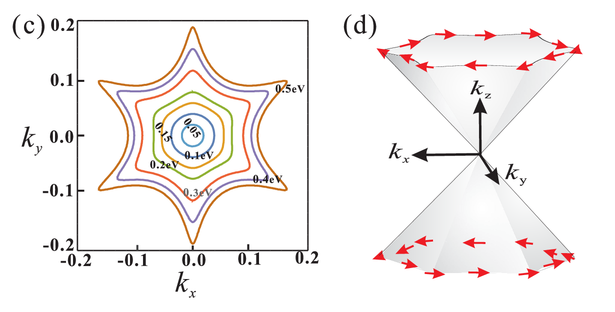
A set of constant energy contours of $H_{0}\left(\mathbf{k}\right)$ are be obtained, as plotted in Fig. 2(c), where we have taken $\lambda=250\,\text{eV}{\AA}^{3}$ and $v_{F}\hbar=2.25\,{\color[rgb]{0,0,1}{\text{eV}{\AA}}}$ for Bi₂Te₃ Fu. When the Fermi energy gets close to the Dirac point ($E=0$ eV), the Fermi surface manifests itself as a circle and the warping effect is inapparent. The Fermi surface starts to deviate considerably from a circle and becomes more hexagonalike around $E=0.2$ eV.

Figs. 2(a) and (b) illustrate the dependence of nonlinear spin Nernst current (NSNC) $\left[\mathbf{j}^{s}_{nl}\right]^{x}_{y}$ on the Fermi energy and the hexagonal warping effect. A larger $\left[\mathbf{j}^{s}_{nl}\right]^{x}_{y}$ can be generated by increasing the hexagonal warping parameters and the absolute value of the Fermi energy in which the hexagonal warping effect will be enhanced. An interesting finding is that in addition to the contribution of hexagonal warping term, the linear-$k$ Dirac dispersion ($\lambda=0$) can also give rise to the signal of nonlinear spin Nernst current, which is distinguished from the electric-field-induced nonlinear spin Hall currentPan2. This can explain why the NSNC is nonzero when the energy is in the range of [0 eV, 0.2eV] [Fig. 2(a)], in which the trigonal warping effect is insignificant [Fig. 2(c)]. However, the signal of NSNC originated from the linear-$k$ Dirac dispersion cannot be converted into the nonlinear planar Nernst current when the Fermi energy is away from the Dirac point (see the details in Sec. III and Appendix D.1).

In the absence of magnetic field, the carriers with opposite spins are equally populated and move in opposite directions in transverse direction ($y$-direction) [Fig. 1(f)]. Hence, there is no charge current flux vertical to temperature gradient. However, when applying an in-plane magnetic field to the topological insulator, because of the spin-momentum locking, the Fermi surface will be distorted in the direction perpendicular to magnetic field [Figs. 1(c) and (d)] due to the hexagonal warping term, which leads to the imbalance between the two spin fluxes of the spin current and thus, the spin current is partially converted into the nonlinear planar Nernst current (NPNC) [Fig. 1(g)].

It should be emphasized that the successful conversion from the spin current into NPNC is ensured by the hexagonal warping effect. If there is no hexagonal warping term, i.e., $\lambda=0$, the energy dispersion turns into the linear-$k$ Dirac dispersion and the Fermi surface returns to a circle. Instead of being distorted, pervious studies K.Yasuda1; Xiao-Qin-1 show that the whole linear dispersion will shift in the momentum space when applying an in-plane magnetic field. Thus, the spin population will stay the same and the two spin fluxes still keep the balance, hinting that there is no NPNC in this case. However, one might notice that there is very weak signal (almost $500$ times smaller than the sign from the warping effect, see Fig.3(a)) stemmed from the linear dispersion when the Fermi energy is located near Dirac point within $10k_{B}T$. This weak signal can be attributed to the temperature broadening effect (see Appendix D.1 for a detailed discussion).

In the presence of a magnetic field $\mathbf{B}$, the effective Hamiltonian for the surface state of topological insulator Bi₂Te₃ Fu is given by

where $g$ and $\mu_{B}$ represent the $g$-factor and Bohr magneton, respectively. The energy eigenvalues are

In the following, we shall consider the upper surface bands, namely $n=1$, and write $\epsilon^{\text{M}}_{n=1}\left(\mathbf{k}\right)$ as $\epsilon^{\text{M}}_{\mathbf{k}}$ for simplicity. The lower surface bands can be analysed in the similar way.

The charge current $j_{a}$ in $a$-direction is $j_{a}=-e\int[d\mathbf{k}]v_{a}f(\mathbf{r},\mathbf{k})$. After tedious derivation in Appendix B, the current $j_{a}^{\left(1\right)}$ and $j_{a}^{\left(2\right)}$ as the first-order and second-order responses to the temperature gradient in the first-order approximation of magnetic field are found, respectively, to be

where the relation $\partial\epsilon_{\mathbf{k}}^{\text{M}}/\partial B_{d}=g\mu_{B}\partial\epsilon_{\mathbf{k}}^{\text{M}}/\partial h_{d}$ has been applied. Explicit expressions for the linear current response ($G_{ab}$, $K_{abc}$) and nonlinear response function ($W_{abc}$, $Q_{abcd}$) are given in Eqs. () and (B16).

Through exploiting the parity in Table 1, one can find the following tensor elements are zero, i.e.,

which suggest that when applying an in-plane magnetic field $\mathbf{B}=B(\cos\theta,\sin\theta)$ and temperature gradient $\partial_{x}T$ along $x$-direction (i.e., $b=c=x$), the planar Nernst effect $j^{\left(1\right)}_{a}$ disappears in Bi₂Te₃ and has no contribution to the transverse thermal voltage signal. And the current density $j^{\left(2\right)}_{y}$ flowing along the $y$-direction (i.e., $d=y$) as the response to the second order in temperature gradient stems from the nonlinear planar Nernst current density $j^{\text{p}}_{nl}$ (where the subscript “nl” and superscript “p” denote nonlinear and planar, respectively) and is found to be

where the nonlinear planar coefficient $Q_{yxxx}$ is given as

where the coefficients $\Upsilon_{1}$,$\Upsilon_{2}$,$\Upsilon_{3}$ and $\Upsilon_{4}$ are given in Eq. (B19).

Eq. (11) indicates the nonlinear planar current $j^{\text{p}}_{nl}$ exhibits $\cos\theta$ dependence on the orientation of magnetic field and is proportional to the $x$-component of the magnetic field $B_{x}\propto B\cos\theta$. Thus, when the magnetic field is collinear with the temperature gradient (i.e., $\theta=0,\pi,2\pi$), the magnitude of $\mid j^{\text{p}}_{nl}\mid$ will reach its maximum. However, the nonlinear planar Nernst effect will disappear when the magnetic field $\mathbf{B}$ is vertical to the temperature gradient. These features of the nonlinear planar Nernst current depending on the orientation of magnetic field can be ascribed to the spin-momentum locking. As shown in Fig. 1(f) and discussion in Sec. II, the spin orientation in the nonlinear spin Nernst current generated by temperature gradient $\nabla_{x}T$ is along $x$-direction. Therefore, only the $x$-component of magnetic field can lead to a transition between the two spin currents and induces the imbalance of two spin carriers [Fig. 1(e)]. As a result the nonlinear spin Nernst current will be partially converted to nonlinear planar Nernst current [Figs. 1(f) and (g)].

We use the following parameters for Bi₂Te₃: the Fermi velocity $v_{F}\hbar=2.25\,\text{eV}{\AA}$, $g=2$, and the scattering relaxation time $\tau\approx 5.864\times 10^{-13}s$ is estimated by $\tau=\mu m/e$. The mobility of surface states in Bi₂Te₃ can range from $9\times 10^{3}$ to $10^{4}$ cm²V^-1s^-1.Qu $\mu=9000$ cm²V^-1s^-1 is used for an estimation.

It’s observed that a very weak signal appears near the Dirac point with a few $k_{B}T$, and $Q_{yxxx}$ is almost zero when the energy is in the range of [0, 0.2eV], as expected, since the trigonal warping effect is insignificant and the Fermi surface almost displays like a circle [Fig. 2(c)] in this range. The appearance of faint signal at the Dirac point can attributes to the thermal broadening effect of nonequilibrium Fermi distribution near Dirac point for the linear-$k$ Dirac dispersion [the details can be found in Appendix D.1]. Besides, one might notice that the signal of $Q_{yxxx}$ is still quite weak when the Fermi energy is in the range of [0.2, 0.4] eV, a regime where a warped Fermi surface is present [Fig. 2] (c). This can be attributed to the low conversion efficiency from the nonlinear spin to charge current [Fig. c1]. However, when the absolute value of Fermi energy $|E_{f}|$ is increased sufficiently, the trigonal warping effect will become profound and lead to a large enhancement of nonlinear planar Nernst effect. It is interesting to point out that the impact of varying temperature is negligible [Fig. 3(a) (b)] when Fermi energy is away from Dirac point. Figure 3(c) and $(d)$ present the Fermi energy and hexagonal warping dependence of $Q_{yxxx}$. The magnitude of $Q_{yxxx}$ increases monotonously with the enhanced energy warping parameter $\lambda$. As expected, when $\lambda$ tends to be zero, the nonlinear planar Nernst effect will disappear.

To numerically estimate the proposed effect, we take $Q_{yxxx}\approx 0.8\,\text{nA}\cdot\mu\text{m}/\text{T K}^{2}$ [Fig. 3(b)] for $T=30\text{K}$ and $E_{f}=0.5\,eV$. In experiment, the temperature gradient can already reach $1\,\text{K}\mu\text{m}^{-1}$.Xu Therefore, when applying the magnetic field $B=3\text{T}$ parallel to temperature gradient, the nonlinear planar Nernst current $j^{\text{P}}_{nl}\times l$ [Eq. (11)] of Bi₂Te₃ is estimated to be order of $0.16\,\mu\text{A}$ with the length of sample $l=50\,\mu m$, which is measurable.

A Rashba-split surface states in two-dimensional electron gas (2DEG) Y.Wang; Mellnik; Denkert [Fig. D3(d)] might coexists with topological surfaces states (TSS) due to the surface band bending in topological insulators, which may also have a significant contribution to the nonlinear Planar Nernst effect. However, it is found that only when Fermi energy locates near the Lifshitz point within a few $k_{B}T$, a very weak signal ($100$ times smaller than the signal arising from TSS) can be generated [see the details in Appendix D.3]. Therefore, the contribution of Rashba 2DEG to NPNE can be neglected.

In summary, we propose a new effect, i.e. the nonlinear planar Nernst effect (NPNE) in this work. It is found that a nonlinear spin-Nernst current, originated from the hexagonal warping effect and the nonequilibrium carrier distribution, flows transversely to temperature gradient direction and can be partially converted into the nonlinear-planar-Nernst current $j^{\text{p}}_{nl}$ when an in-plane magnetic field is applied to TI. The quantity of $j^{\text{p}}_{nl}$ is strongly dependent on the orientation of the magnetic field. When the in-plane magnetic field is collinear to the temperature gradient, $|j^{\text{p}}_{nl}|$ will reach its maximum. However, $j^{\text{p}}_{nl}$ becomes zero when the magnetic field is perpendicular to the temperature gradient. The magnitude of NPNE is strongly affected by the hexagonal warping term and the Fermi energy. Except a very faint signal of NPNE appearing near the Dirac point within a few $k_{B}T$ due to the temperature broadening effect, when the Fermi level is close to the Dirac point, the signal of the NPNE mostly disappears due to the weak hexagonal warping effect. However, when enlarging the value $|E_{f}|$ sufficiently, the NPNE rapidly increases owing to the profound hexagonal warping effect. The nonlinear planar Nernst effect proposed here might also occur in other noncentrosymmetric materials with strong spin-orbit coupling and nontrivial spin textures. Therefore, our findings have great potential application in magneto-thermal transport and spin caloritronics, and might pave a new way to the emerging field of nonlinear spin caloritronics.

This work is supported by the Fundamental Research Funds for the Central Universities and the NSFC (Grant No.12004107). G.S. and Z.G.Z. are supported in part by the National Key R&D Program of China (Grant No. 2018FYA0305800), the Strategic Priority Research Program of CAS (Grant Nos. XDB28000000), the NSFC (Grant No. 11834014), and Beijing Municipal Science and Technology Commission (Grant No. Z118100004218001). Z.G.Z. is also supported in part by the NSFC (Grant Nos. 11674317 and 11974348).

References

- (1) M. Z. Hasan and C. L. Kane, Rev. Mod. Phys. 82, 3045 (2010).
- (2) X.-L. Qi and S. C. Zhang, Rev. Mod. Phys. 83, 1057 (2011).
- (3) Y. Shiomi, K. Nomura, Y. Kajiwara, K. Eto, M. Novak, K. Segawa, Y. Ando, and E. Saitoh, Phys. Rev. Lett. 113, 196601 (2014).
- (4) Z. Jian, C.-Z. Chang, M. R. Masir, C. Tang, Y. Xu, J. S. Moodera, A. H. MacDonald, and J. Shi, Nat. Commun. 7, 11458 (2016).
- (5) H. Wang, J. Kally, J. Sue Lee, T. Liu, H. Chang, D. R. Hickey, K. A. Mkhoyan, M. Wu, A. Richardella, and N. Smarth, Phys. Rev. Lett. 117, 076601 (2016).
- (6) J. Han, A. Richardella, S. A. Siddiqui, J. Finley, N. Samarth, and L. Liu, Phys. Rev. Lett. 119, 077702 (2017).
- (7) Y. Wang£¬D. Zhu, Y. Wu, Y. Yang, J. Yu, R. Ramaswamy, R. Mishra, S. Shi, M. Elyasi, K.-L. Teo, Y. Wu, and H. Yang Nat. Commun. 8, 1364 (2017).
- (8) M. Dc, R. Grassi, J.-Y. Chen, M. Jamali, D. R. Hickey, D. Zhang, Z. Zhao, H. Li, P. Quarterman, Y. Lv, M. Li, A. Manchon, K. A. Mkhoyan, T. Low, and J.-P. Wang, Nat. Mater. 17, 800 (2018).
- (9) C. -F. Pai, Nat. Mater. 17, 755 (2018).
- (10) X. Wang, Y. Du, S. Dou and C. Zhang, Phys. Rev. Lett. 108, 266806 (2012).
- (11) J. Wang, H. Li, C. Chang, K. He, J. S. Lee, H. Lu, Y. Sun, X. Ma, N. Samarth, S. Shen, Q. Xue, M. Xie, and M. H. W. Chan, Nano Res. 5, 739-746 (2012).
- (12) A. Sulaev, M. Zeng, S.-Q. Shen, S. K. Cho, W. G. Zhu, Y. P. Feng, S. V. Eremeev, Y. Kawazoe, L. Shen, and L. Wang, Nano lett. 15, 2061-2066 (2015).
- (13) S. Wiedmann, A. Jost, B. Fauqué, J. van Dijk, M. J. Meijer, T. Khouri, S. Pezzini, S. Grauer, S.Schreyeck, C. Br¨¹ne, H. Buhmann, L. W. Molenkamp, and N. E. Hussey Phys. Rev. B 94, 081302 (R) (2016).
- (14) A. A. Taskin, H. F. Legg, F. Yang, S. Sasaki, Y. Kanai, K. Matsumoto, A. Rosch, and Y. Ando, Nat. Commun. 8, 1340 (2017).
- (15) P. He, S. S. L. Zhang, D. Zhu, Y. Liu, Y. Wang, J. Yu, G. Vignale, and H. Yang, Nat. Phys. 14, 495 (2018).
- (16) A. Dyrdal, J. Barnaś, and A. Fert, Phys. Rev. Lett. 124, 046802 (2020).
- (17) C. O. Avci, K. Garello, A. Ghosh, M. Gabureac, S. F. Alvarado, and P. Gambardella, Nat. Phys. 11, 570 (2015).
- (18) C. O. Avci, K. Garello, J. Mendil, A. Ghosh, N. Blsakis, M. Gabureac, M. Trassin, M. Fiebig, and P. Gambardella, App. Phys. Lett. 107, 192405 (2015).
- (19) S. Langenfeld, V. Tshitoyan, Z. Fang, A. Wells, T. A. Moore, and A. J. Ferguson, App. Phys. Lett. 108, 192402 (2016).
- (20) K. Yasuda, A. Tsukazaki, R. Yoshimi, K. S. Takahashi, M. Kawasaki, and Y. Tokura, Phys. Rev. Lett. 117, 127202 (2016).
- (21) Y. Lv, J. Kally, D.Zhang, J. S. Lee, M. Jamali, N. Samarth and J.-P. Wang, Nat. Commun. 9, 111 (2018).
- (22) A. A. Taskin, S. Sasaki, K. Segawa, and Y. Ando, Phys. Rev. Lett. 109, 066803 (2012).
- (23) B. Wu, X.-C. Pan, W. Wu, F. Fei, B. Chen, Q. Liu, H. Bu, L. Cao, F. Song, and B. Wang, Appl. Phys. Lett. 113, 011902(2018).
- (24) D. Rakhmilevich, F. Wang, W. Zhao, M. H. W. Chan, J. S. Moodera, C. Liu, and C.-Z. Chang, Phys. Rev. B 98, 094404 (2018).
- (25) S.-H. Zhang. H.-J. Duan, J.-K. Wang, J.-Y. Li, M.-X. Deng, and R.-Q. Wang, Phys. Rev. B 101, 041408(R) (2020).
- (26) P. He, S. S.-L. Zhang, D. Zhu, S. Shi, and O. G. Heinonen, Phys. Rev. Lett. 123, 016801 (2019).
- (27) X.-Q. Yu, Z.-G. Zhu, and G. Su, Phys. Rev. B 100, 195418 (2019).
- (28) X.-Q. Yu, Z.-G. Zhu, J.-S. You, T. Low, and G. Su, Phys. Rev. B 99, 201410(R) (2019).
- (29) C. Zeng, S. Nandy, A. Taraphder, and S. Tewari, Phys. Rev. B 100, 245102 (2019).
- (30) G. E. W. Bauer, E. Saitoh, and B. J. van Wees, Nat. Mater. 11, 391 (2012).
- (31) A. D. Avery, M. R. Pufall, and B. L. Zink, Phys. Rev. Lett. 109, 196602 (2012).
- (32) S. Y. Huang, W. G. Wang, S. F. Lee, J. Kwo, and C. L. Chien, Phys. Rev. Lett. 107, 216604 (2011).
- (33) S. R. Boona, R. C. Myersbc and J. P. Heremans, Energy Environ. Sci , 7, 885-910 (2014).
- (34) X.-Q. Yu, Z.-G. Zhu, G. Su, and A.-P. Jauho, Phys. Rev. Lett. 115, 246601 (2015).
- (35) V. Baltz, A. Manchon, M. Tsoi, T. Moriyama, T. Ono, and Y. Tserkovnyak, Rev. Mod. Phys. 90, 015005 (2018).
- (36) L. Fu, Phys. Rev. Lett. 103, 266801 (2009).
- (37) C. M. Wang and X. L. Lei, Phys. Rev. B 89, 045415 (2014).
- (38) Dong-Xia Qu, Y. S. Hor, Jun Xiong, R. J. Cava, and N. P. Ong, Science 329, 5993 (2010).
- (39) J. Xu, W. A. Phelan, and C.-L. Chien, Nano Lett. 19, 8250-8254 (2019).
- (40) Y. Wang, P. Deorani, K. Banerjee, N. Koirala, M. Brahlek, S. Oh, and H. Yang, Phys. Rev. Lett. 114, 257202 (2015).
- (41) A. R. Mellnik et al., Nature (London) 511, 449 (2014).
- (42) A. Dankert, J. Geurs, M. V. Kamalakar, S. Charpentier, and S. P. Dash, Nano Lett. 15, 7976 (2015).
- (43) J. M. Ziman, Electrons and Phonons: The Theory of Transport phenomena in Solid (Oxford University Press, New York, 1960).
- (44) H.-J. Zhang, C.-X. Liu, X.-L. Qi, X. Dai, Z. Fang, and S.-C. Zhang, Nat. Phys. 5, 438 (2009).
- (45) C.-X. Liu, X.-L. Qi, H. J. Zhang, X. Dai, Z. Fang, and S.-C.Zhang, Phys. Rev. B 82, 045122 (2010).