Scale-free Protocol Design for Output and Regulated Output Synchronization of Heterogeneous Multi-agent Systems

Donya Nojavanzadeh Zhenwei Liu Ali Saberi Anton A. Stoorvogel Thanks: Donya Nojavanzadeh is with School of Electrical Engineering and Computer Science, Washington State University, Pullman, WA 99164, USA donya.nojavanzadeh@wsu.edu Thanks: Zhenwei Liu is with College of Information Science and Engineering, Northeastern University, Shenyang 110819, P. R. China jzlzwsy@gmail.com Thanks: Ali Saberi is with School of Electrical Engineering and Computer Science, Washington State University, Pullman, WA 99164, USA saberi@eecs.wsu.edu Thanks: Anton A. Stoorvogel is with Department of Electrical Engineering, Mathematics and Computer Science, University of Twente, P.O. Box 217, Enschede, The Netherlands A.A.Stoorvogel@utwente.nl

Abstract

In this paper, we consider scalable output and regulated output synchronization problems for heterogeneous networks of right-invertible linear agents based on localized information exchange where in the case of regulated output synchronization, the reference trajectory is generated by a so-called exosystem. We assume that all the agents are introspective, meaning that they have access to their own local measurements. We propose a scale-free linear protocol for each agent to achieve output and regulated output synchronizations. These protocols are designed solely based on agent models and they need no information about communication graph and the number of agents or other agent models information.

I Introduction

Synchronization problem of multi-agent systems (MAS) has become a hot topic among researchers in recent years. Cooperative control of MAS is used in practical application such as robot network, autonomous vehicles, distributed sensor network, and others. The objective of synchronization is to secure an asymptotic agreement on a common state or output trajectory by local interaction among agents (see [1, 10, 19, 24] and references therein).

State synchronization inherently requires homogeneous networks. Most works have focused on state synchronization where each agent has access to a linear combination of its own state relative to that of the neighboring agents, which is called full-state coupling [12, 13, 14, 17, 18, 20]. A more realistic scenario which is partial-state coupling (i.e. agents share part of their information over the network) is studied in [21, 9, 15, 22].

For heterogeneous network it is more reasonable to consider output synchronization since the dimensions of states and their physical interpretation may be different. Introspective agents possess some knowledge about their own states. For heterogeneous MAS with non-introspective agents, it is well-known that one needs to regulate outputs of the agents to a priori given trajectory generated by a so-called exosystem (see [23, 4]). Other works on synchronization of MAS with non-introspective agents can be found in the literature as [6, 5].

On the other hand, for MAS with introspective agents, one can achieve output and regulated output synchronization. Most of the literature for heterogeneous MAS with introspective agents are based on modifying the agent dynamics via local feedback to achieve some form of homogeneity. There have been many results for synchronization of heterogeneous networks with introspective agents, see for instance [7, 25, 8, 11, 16, 2].

In this paper, we propose scale-free protocol design to solve output and regulated output synchronization problems for heterogeneous MASs with introspective right-invertible agents. Scale-free protocols are designed based on localized information exchange with neighbors and do not require any knowledge of the communication network except connectivity. The protocol design is scale-free, namely,

$\bullet$

The design is independent of the information about communication networks such as spectrum of the associated Laplacian matrix. That is to say, the universal dynamical protocols work for any communication network as long as it is connected.
$\bullet$

The dynamic protocols are designed solely based on agent models and do not depend on communication network and the number of agents.
$\bullet$

The proposed protocols achieve output and regulated output synchronization for heterogeneous MAS with any number of agents and any communication network.

Notations and definitions

Given a matrix $A\in\mathbb{R}^{m\times n}$ , $A^{\mbox{\tiny T}}$ denotes its conjugate transpose. A square matrix $A$ is said to be Hurwitz stable if all its eigenvalues are in the open left half complex plane. We denote by $\diag\{A_{1},\ldots,A_{N}\}$ , a block-diagonal matrix with $A_{1},\ldots,A_{N}$ as its diagonal elements. $A\otimes B$ depicts the Kronecker product between $A$ and $B$ . $I_{n}$ denotes the $n$ -dimensional identity matrix and $0_{n}$ denotes $n\times n$ zero matrix; sometimes we drop the subscript if the dimension is clear from the context.

To describe the information flow among the agents we associate a weighted graph $\mathcal{G}$ to the communication network. The weighted graph $\mathcal{G}$ is defined by a triple $(\mathcal{V},\mathcal{E},\mathcal{A})$ where $\mathcal{V}=\{1,\ldots,N\}$ is a node set, $\mathcal{E}$ is a set of pairs of nodes indicating connections among nodes, and $\mathcal{A}=[a_{ij}]\in\mathbb{R}^{N\times N}$ is the weighted adjacency matrix with non negative elements $a_{ij}$ . Each pair in $\mathcal{E}$ is called an edge, where $a_{ij}>0$ denotes an edge $(j,i)\in\mathcal{E}$ from node $j$ to node $i$ with weight $a_{ij}$ . Moreover, $a_{ij}=0$ if there is no edge from node $j$ to node $i$ . We assume there are no self-loops, i.e. we have $a_{ii}=0$ . A path from node $i_{1}$ to $i_{k}$ is a sequence of nodes $\{i_{1},\ldots,i_{k}\}$ such that $(i_{j},i_{j+1})\in\mathcal{E}$ for $j=1,\ldots,k-1$ . A directed tree is a subgraph (subset of nodes and edges) in which every node has exactly one parent node except for one node, called the root, which has no parent node. A directed spanning tree is a subgraph which is a directed tree containing all the nodes of the original graph. If a directed spanning tree exists, the root has a directed path to every other node in the tree [3].

For a weighted graph $\mathcal{G}$ , the matrix $L=[\ell_{ij}]$ with

\ell_{ij}=\left\{\;\begin{array}[]{cl}\sum_{k=1}^{N}a_{ik},&i=j,\\ -a_{ij},&i\neq j,\end{array}\right.

is called the Laplacian matrix associated with the graph $\mathcal{G}$ . The Laplacian matrix $L$ has all its eigenvalues in the closed right half plane and at least one eigenvalue at zero associated with right eigenvector 1 [3].

II Problem Formulation

We will study a MAS consisting of $N$ non-identical linear agents:

\begin{array}[]{cl}\dot{x}_{i}&=A_{i}x_{i}+B_{i}u_{i},\\ y_{i}&=C_{i}x_{i},\end{array}

(1)

where $x_{i}\in\mathbb{R}^{n_{i}}$ , $u_{i}\in\mathbb{R}^{m_{i}}$ and $y_{i}\in\mathbb{R}^{p}$ are the state, input, output of agent $i$ for $i=1,\ldots,N$ .

The agents are introspective, meaning that each agent has access to its own local information. Specifically each agent has access to part of its state

z_{i}=C_{i}^{m}x_{i}.

(2)

where $z_{i}\in\mathbb{R}^{q_{i}}$ .

The communication network provides agent $i$ with the following information which is a linear combination of its own output relative to that of other agents:

\zeta_{i}=\sum_{j=1}^{N}a_{ij}(y_{i}-y_{j})

(3)

where $a_{ij}>0$ and $a_{ii}=0$ . The communication topology of the network can be described by a weighted and directed graph $\mathcal{G}$ with nodes corresponding to the agents in the network and the weight of edges given by the coefficient $a_{ij}$ . In terms of the coefficients of the associated Laplacian matrix $L$ , $\zeta_{i}$ can be rewritten as

\zeta_{i}=\sum_{j=1}^{N}\ell_{ij}y_{j}.

(4)

In this paper, we also introduce a localized information exchange among agents, namely, each agent $i\in\{1,...,N\}$ has access to localized information, denoted by $\hat{\zeta}_{i}$ , of the form

\hat{\zeta}_{i}=\sum_{j=1}^{N}a_{ij}(\eta_{i}-\eta_{j})

(5)

where $\eta_{i}$ is a variable produced internally by agent $i$ and to be defined later.

In order to explicitly state our problem formulation we need the following definition.

Definition 1

Let $\mathbb{G}^{N}$ denote the set of directed graphs of $N$ agents which contain a directed spanning tree.

Now we formulate the problem of scalable output synchronization for a heterogeneous MAS.

Problem 1

Consider a heterogeneous network of $N$ agents (1) with local information (2) satisfying Assumption 1. Let the associated network communication be given by (4). Let $\mathbb{G}^{N}$ be the set of network graphs as defined in Definition 1. The scalable output synchronization problem based on localized information exchange is to find, if possible, a linear dynamic controller for each agent $i\in\{1,\dots,N\}$ , using only knowledge of agent models, i.e. $(C_{i},A_{i},B_{i})$ , of the form:

\left\{\;\begin{array}[]{cl}\dot{x}_{i,c}&=A_{i,c}x_{i,c}+B_{i,c}\zeta_{i}+C_{i,c}\hat{\zeta}_{i}+D_{i,c}z_{i},\\ u_{i}&=E_{i,c}x_{i,c}+F_{i,c}\zeta_{i}+G_{i,c}\hat{\zeta}_{i}+H_{i,c}z_{i},\end{array}\right.

(6)

where $\hat{\zeta}_{i}$ is defined in (5) with $\eta_{i}=M_{i,c}x_{i,c}$ , and $x_{c,i}\in\mathbb{R}^{n_{i}}$ , such that output synchronization

\lim\limits_{t\to\infty}(y_{i}(t)-y_{j}(t))=0

(7)

is achieved for any $N$ and any graph $\mathcal{G}\in\mathbb{G}^{N}$ .

Next, we consider regulated output synchronization where output of agents converge to a priori given trajectory $y_{r}$ generated by a so-called exosystem as

\begin{array}[]{cl}\dot{x}_{r}&=A_{r}x_{r},\quad x_{r}(0)=x_{r0},\\ y_{r}&=C_{r}x_{r},\end{array}

(8)

where $x_{r}\in\mathbb{R}^{r}$ and $y_{r}\in\mathbb{R}^{p}$ .

We assume a nonempty subset $\mathscr{C}$ of the agents which have access to their output relative to the output of the exosystem. In other word, each agent $i$ has access to the quantity

\Psi_{i}=\iota_{i}(y_{i}-y_{r}),\qquad\iota_{i}=\left\{\;\begin{array}[]{cl}1,\quad i\in\mathscr{C},\\ 0,\quad i\notin\mathscr{C}.\end{array}\right.

(9)

By combining this with (3), the information exchange among agents is given by

\tilde{\zeta}_{i}=\sum_{j=1}^{N}a_{ij}(y_{i}-y_{j})+\iota_{i}(y_{i}-y_{r}).

(10)

$\tilde{\zeta}_{i}$ as defined in above, can be rewritten in terms of the coefficients of a so-called expanded Laplacian matrix $\tilde{L}=L+diag\{\iota_{i}\}=[\tilde{\ell}_{ij}]_{N\times N}$ as

\tilde{\zeta}_{i}=\sum_{j=1}^{N}\tilde{\ell}_{ij}(y_{j}-y_{r}).

(11)

Note that $\tilde{L}$ is not a regular Laplacian matrix associated to the graph, since the sum of its rows need not be zero. We know that all the eigenvalues of $\tilde{L}$ , have positive real parts. In particular matrix $\tilde{L}$ is invertible.

To guarantee that each agent gets the information from the exosystem, we need to make sure that there exists a path from node set $\mathscr{C}$ to each node. Therefore, we define the following set of graphs.

Definition 2

Given a node set $\mathscr{C}$ , we denote by $\mathbb{G}_{\mathscr{C}}^{N}$ the set of all graphs with $N$ nodes containing the node set $\mathscr{C}$ , such that every node of the network graph $\mathcal{G}\in\mathbb{G}_{\mathscr{C}}^{N}$ is a member of a directed tree which has its root contained in the node set $\mathscr{C}$ . We will refer to the node set $\mathscr{C}$ as root set.

Remark 1

Note that Definition 2 does not require necessarily the existence of directed spanning tree.

Now we formulate the problem of scalable regulated output synchronization for a heterogeneous MAS.

Problem 2

Consider a heterogeneous network of $N$ agents (1) with local information (2) satisfying Assumption 1 and the associated exosystem (8) satisfying Assumption 2. Let a set of nodes $\mathscr{C}$ be given which defines the set $\mathbb{G}^{N}_{\mathscr{C}}$ . Let the associated network communication be given by (11). The scalable regulated output synchronization problem based on localized information exchange is to find, if possible, a linear dynamic controller for each agent $i\in\{1,\dots,N\}$ , using only knowledge of agent models, i.e. $(C_{i},A_{i},B_{i})$ , of the form:

\left\{\;\begin{array}[]{cl}\dot{x}_{i,c}&=A_{i,c}x_{i,c}+B_{i,c}\tilde{\zeta}_{i}+C_{i,c}\hat{\zeta}_{i}+D_{i,c}z_{i},\\ u_{i}&=E_{i,c}x_{i,c}+F_{i,c}\tilde{\zeta}_{i}+G_{i,c}\hat{\zeta}_{i}+H_{i,c}z_{i},\end{array}\right.

(12)

where $\hat{\zeta}_{i}$ is defined in (5) with $\eta_{i}=M_{i,c}x_{i,c}$ , and $x_{c,i}\in\mathbb{R}^{n_{i}}$ , such that regulated output synchronization

\lim\limits_{t\to\infty}(y_{i}(t)-y_{r}(t))=0

(13)

is achieved for any $N$ and any graph $\mathscr{G}\in\mathbb{G}^{N}_{\mathscr{C}}$ .

In this paper, we make the following assumptions for agents and the exosystem.

Assumption 1

For agents $i\in\{1,\dots,N\}$ ,

1.

$(C_{i},A_{i},B_{i})$ is stabilizable, detectable and right-invertible.
2.

$(C_{i}^{m},A_{i})$ is detectable.

Assumption 2

For exosystem,

1.

$(C_{r},A_{r})$ is observable.
2.

All the eigenvalues of $A_{r}$ are on the imaginary axis.

III Scalable Output Synchronization

In this section, we design protocols to solve scalable output synchronization problem as stated in Problem 1. After introducing the architecture of our protocol, we design the protocols through four steps.

III-A Architecture of the protocol

Our protocol has the structure shown below in Figure 1.

Refer to caption — Figure 1: Architecture of the protocol for output synchronization

As seen in the above figure, our design methodology consists of two major modules.

1.

The first module is reshaping the dynamics of the agents to obtain the target model by designing pre-compensators following our previous results in [25].
2.

The second module is designing collaborate protocols for almost homogenized agents to achieve output and regulated output synchronization

III-B Protocol design

We design our protocols through the following four steps.

Step 1: choosing target model First, we choose the suitable target model, i.e. $(C,A,B)$ such that the following conditions are satisfied.

1.

$\rank(C)=p$
2.

$(C,A,B)$ is invertible of uniform rank $n_{q}\geq\bar{n}_{d}$ , and has no invariant zeros, where $\bar{n}_{d}$ denotes the maximal order of infinite zeros of $(C_{i},A_{i},B_{i}),i=1,\ldots,N$ .
3.

eigenvalues of $A$ are in closed left half plane.

Step 2: designing pre-compensators In this step, we design pre-compensators to reshape agent models to almost identical agents. Given chosen target model $(C,A,B)$ , by utilizing the design methodology from [25, Appendix B], we design a pre-compensator for each agent $i\in\{1,\dots,N\}$ , of the form

\left\{\;\begin{array}[]{cl}\dot{\xi}_{i}&=A_{i,h}\xi_{i}+B_{i,h}z_{i}+E_{i,h}v_{i},\\ u_{i}&=C_{i,h}\xi_{i}+D_{i,h}v_{i},\end{array}\right.

(14)

which yields the compensated agents as

\begin{array}[]{cl}\dot{\bar{x}}_{i}&=A\bar{x}_{i}+B(v_{i}+\rho_{i}),\\ {y}_{i}&=C\bar{x}_{i},\end{array}

(15)

where $\rho_{i}$ is given by

\begin{array}[]{cl}\dot{\omega}_{i}&=A_{i,s}\omega_{i},\\ \rho_{i}&=C_{i,s}\omega_{i},\end{array}

(16)

and $A_{i,s}$ is Hurwitz stable. Note that the compensated agents are homogenized and have the target model $(C,A,B)$ .

Step 3: designing collaborative protocols for compensated agents In this step, we design a dynamic protocol based on localized information exchange for compensated agents (15) and (16) as

\left\{\;\begin{array}[]{cl}\dot{\hat{x}}_{i}&=A\hat{x}_{i}-BK\hat{\zeta}_{i}+H(\zeta_{i}-C\hat{x}_{i})\\ \dot{\chi}_{i}&=A\chi_{i}+Bv_{i}+\hat{x}_{i}-\hat{\zeta}_{i}\\ v_{i}&=-K\chi_{i}\end{array}\right.

(17)

where $H$ and $K$ are matrices such that $A-HC$ and $A-BK$ are Hurwitz stable. The agents communicate $\eta_{i}$ which is chosen as $\eta_{i}=\chi_{i}$ . Therefore, each agent has access to the following information:

\hat{\zeta}_{i}=\sum_{j=1}^{N}a_{ij}(\chi_{i}-\chi_{j}),

(18)

and $\zeta_{i}$ is defined as (4).

Step 4: obtaining protocols for the agents Finally, our protocol which is the combination of module $1$ and $2$ is as following.

\left\{\;\begin{array}[]{cl}\dot{\xi}_{i}&=A_{i,h}\xi_{i}+B_{i,h}z_{i}-E_{i,h}K\chi_{i},\\ \dot{\hat{x}}_{i}&=A\hat{x}_{i}-BK\hat{\zeta}_{i}+H(\zeta_{i}-C\hat{x}_{i})\\ \dot{\chi}_{i}&=A\chi_{i}-BK\chi_{i}+\hat{x}_{i}-\hat{\zeta}_{i}\\ u_{i}&=C_{i,h}\xi_{i}-D_{i,h}K\chi_{i},\end{array}\right.

(19)

Then, we have the following theorem for output synchronization of heterogeneous MAS.

Theorem 1

Consider a heterogeneous network of $N$ agents (1) with local information (2) satisfying Assumption 1. Let the associated network communication be given by (4). Then, the scalable output synchronization problem as defined in Problem 1 is solvable. In particular, the dynamic protocol (19) with localized information (18) solves the scalable output synchronization problem based on localized information exchange for any $N$ and any graph $\mathcal{G}\in\mathbb{G}^{N}$ .

Remark 2

It is interesting to note that for the case that agents are homogeneous and non-introspective one does not require designing pre-compensators, and obviously can achieve scalable output synchronization utilizing collaborative protocols proposed in step $3$ for homogeneous networks as long as the agents eigenvalues are in the closed left half plane.

To obtain this result, we recall the following lemma for Laplacian matrix $L$ .

Lemma 1 ([26])

Let a Laplacian matrix $L\in\mathbb{R}^{N\times N}$ be given associated with a graph that contains a directed spanning tree. We define $\bar{L}\in\mathbb{R}^{(N-1)\times(N-1)}$ as the matrix $\bar{L}=[\bar{\ell}_{ij}]$ with

\bar{\ell}_{ij}=\ell_{ij}-\ell_{Nj}.

Then the eigenvalues of $\bar{L}$ are equal to the nonzero eigenvalues of $L$ .

Proof: We have:

\bar{L}=\begin{pmatrix}I&-\textbf{1}\end{pmatrix}L\begin{pmatrix}I\\ 0\end{pmatrix}

Assume that $\lambda$ is a nonzero eigenvalue of $L$ with eigenvector $x$ , Then

\bar{x}=\begin{pmatrix}I&-\textbf{1}\end{pmatrix}x

where 1 is a vector with all $1$ ’s, satisfies,

\begin{pmatrix}I&-\textbf{1}\end{pmatrix}Lx=\begin{pmatrix}I&-\textbf{1}\end{pmatrix}\lambda x=\lambda\bar{x}

and since $L\textbf{1}=0$ we find that

\bar{L}\bar{x}=\begin{pmatrix}I&-\textbf{1}\end{pmatrix}Lx=\lambda\bar{x}.

This shows that $\lambda$ is an eigenvector of $\bar{L}$ if $\bar{x}\neq 0$ . It is easily seen that $\bar{x}=0$ if and only if $\lambda=0$ . Conversely if $\bar{x}$ is an eigenvector of $\bar{L}$ with eigenvalue $\lambda$ then it is easily verified that

x=L\begin{pmatrix}I\\ 0\end{pmatrix}\bar{x}

is an eigenvector of $L$ with eigenvalue $\lambda$ .

Proof of Theorem 1: Let $\bar{x}_{i}^{o}=\bar{x}_{i}-\bar{x}_{N}$ , $y_{i}^{o}=y_{i}-y_{N}$ , $\hat{x}_{i}^{o}=\hat{x}_{i}-\hat{x}_{N}$ , and $\chi_{i}^{o}=\chi_{i}-\chi_{N}$ . Then, we have

\begin{array}[]{ll}\dot{\bar{x}}_{i}^{o}&=A\bar{x}_{i}^{o}+B(v_{i}-v_{N}+\rho_{i}-\rho_{N}),\\ {y}_{i}^{o}&=C\bar{x}_{i}^{o},\\ \bar{\zeta}_{i}&=\zeta_{i}-\zeta_{N}=\sum_{j=1}^{N-1}\bar{\ell}_{ij}{y}_{j}^{o},\\ \dot{\hat{x}}_{i}^{o}&=A\hat{x}_{i}^{o}-BK(\hat{\zeta}_{i}-\hat{\zeta}_{N})+H(\bar{\zeta}_{i}-C\hat{x}_{i}^{o})\\ \dot{\chi}_{i}^{o}&=A\chi_{i}^{o}+B(v_{i}-v_{N})+\hat{x}_{i}^{o}-\sum_{j=1}^{N-1}\bar{\ell}_{ij}{\chi}_{j}^{o}\\ v_{i}-v_{N}&=-K\chi_{i}^{o}\end{array}

where $\bar{\ell}_{ij}=\ell_{ij}-\ell_{Nj}$ for $i,j=1,\cdots,N-1$ . According to Lemma 1, we have that eigenvalues of $\bar{L}=[\bar{\ell}_{ij}]_{(N-1)\times(N-1)}$ are equal to the nonzero eigenvalues of $L$ . We define

\bar{x}=\begin{pmatrix}\bar{x}_{1}^{o}\\ \vdots\\ \bar{x}_{N-1}^{o}\end{pmatrix},\hat{x}=\begin{pmatrix}\hat{x}_{1}^{o}\\ \vdots\\ \hat{x}_{N-1}^{o}\end{pmatrix},\chi=\begin{pmatrix}\chi_{1}^{o}\\ \vdots\\ \chi_{N-1}^{o}\end{pmatrix},\rho=\begin{pmatrix}\rho_{1}\\ \vdots\\ \rho_{N}\end{pmatrix},\omega=\begin{pmatrix}\omega_{1}\\ \vdots\\ \omega_{N}\end{pmatrix}

then, we have the following closed-loop system:

\left\{\;\begin{array}[]{cl}\dot{\bar{x}}&=(I\otimes A)\bar{x}-(I\otimes BK)\chi+(\Pi\otimes B)\rho\\ \dot{\hat{x}}&=(I\otimes(A-HC))\hat{x}-(\bar{L}\otimes BK)\chi+(\bar{L}\otimes HC)\bar{x}\\ \dot{\chi}&=(I\otimes(A-BK)-\bar{L}\otimes I)\chi+\hat{x}\end{array}\right.

(20)

with $\Pi=\begin{pmatrix}I&-\mathbf{1}\end{pmatrix}$ . By defining $e=\bar{x}-\chi$ and $\bar{e}=(\bar{L}\otimes I)\bar{x}-\hat{x}$ , we can obtain

\begin{array}[]{cl}\dot{\bar{x}}&=(I\otimes(A-BK))\bar{x}+(I\otimes BK)e+(\Pi\otimes B)C_{s}\omega\\ \dot{e}&=(I\otimes A-\bar{L}\otimes I)e+\bar{e}+(\Pi\otimes B)C_{s}\omega\\ \dot{\bar{e}}&=(I\otimes(A-HC))\bar{e}+(\bar{L}\Pi\otimes B)C_{s}\omega\end{array}

(21)

where $C_{s}=diag\{C_{i,s}\}$ for $i=1,\ldots,N$ . We obtain the synchronization result when $\lim_{t\to\infty}\bar{x}\to 0.$ By combining (16) and (21), we have

\begin{pmatrix}\dot{\bar{x}}\\ \dot{e}\\ \dot{\bar{e}}\\ \dot{\omega}\end{pmatrix}=\left(\begin{array}[]{cc}I\otimes(A-BK)&I\otimes BK\\ 0&I_{N-1}\otimes A-\bar{L}\otimes I\\ 0&0\\ 0&0\end{array}\right.\\ \left.\begin{array}[]{cc}0&(\Pi\otimes B)C_{s}\\ I&(\Pi\otimes B)C_{s}\\ I\otimes(A-HC)&(\bar{L}\Pi\otimes B)C_{s}\\ 0&A_{s}\end{array}\right)\begin{pmatrix}\bar{x}\\ e\\ \bar{e}\\ \omega\end{pmatrix}

(22)

where $A_{s}=diag\{A_{i,s}\}$ for $i=1,\ldots,N$ . Since the eigenvalues $\lambda_{1},\ldots,\lambda_{N}$ of $\bar{L}$ have positive real part, we have, we have

(T\otimes I)(I\otimes A-\bar{L}\otimes I)(T^{-1}\otimes I)=I\otimes A-\bar{\Lambda}\otimes I

(23)

for a non-singular transformation matrix $T$ , where (23) is upper triangular Jordan form with $A-\lambda_{i}I$ for $i=1,\cdots,N-1$ on the diagonal. Since all eigenvalues of $A$ are in the closed left half plane, $A-\lambda_{i}I$ is stable. Therefore, all eigenvalues of $I\otimes A-\bar{L}\otimes I$ have negative real part. Moreover, $A_{s}=\diag(A_{i,s})$ and $A-HC$ are Hurwitz stable, thus it implies we just need to prove the stability of $\dot{\bar{x}}=(I\otimes(A-BK))\bar{x}$ based on the structure of (22). Obviously, since $A-BK$ is Hurwitz stable, we have $\bar{x}$ is asymptotically stable, i.e. $\lim_{t\to\infty}\bar{x}_{i}^{o}\to 0$ . Thus, it implies $\lim_{t\to\infty}y_{i}^{o}=y_{i}-y_{N}=C\bar{x}_{i}^{o}\to 0$ which proves the result.

IV Scalable Regulated Output Synchronization

IV-A Architecture of the protocol

The protocol for regulated output synchronization has two main modules as shown in figure 2.

IV-B Protocol design

Similar to scalable output synchronization, for solving scalable regulated output synchronization, our design procedure consists of four steps.

Step 1: remodeling the exosystem First, we remodel the exosystem to arrive at suitable choice for the target model $(\check{C}_{r},\check{A}_{r},\check{B}_{r})$ following the design procedure in [25] summarized in the following lemma.

Lemma 2 ([25])

There exists another exosystem given by:

\begin{array}[]{cl}\dot{\check{x}}_{r}&=\check{A}_{r}\check{x}_{r},\quad\check{x}_{r}(0)=\check{x}_{r0}\\ y_{r}&=\check{C}_{r}\check{x}_{r},\end{array}

(24)

such that for all $x_{r0}\in\mathbb{R}^{r}$ , there exists $\check{x}_{r0}\in\mathbb{R}^{\check{r}}$ for which (24) generate exactly the same output $y_{r}$ as the original exosystem (8). Furthermore, we can find a matrix $\check{B}_{r}$ such that the triple $(\check{C}_{r},\check{A}_{r},\check{B}_{r})$ is invertible, of uniform rank $n_{q}$ , and has no invariant zero, where $n_{q}$ is an integer greater than or equal to maximal order of infinite zeros of $(C_{i},A_{i},B_{i}),i\in\{1,...,N\}$ and all the observability indices of $(C_{r},A_{r})$ . Note that the eigenvalues of $\check{A}_{r}$ consists of all eigenvalues of $A_{r}$ and additional zero eigenvalues.

Step 2: designing pre-compensators Next, given the target model $(\check{C}_{r},\check{A}_{r},\check{B}_{r})$ , we design pre-compensators to achieve almost identical models as in step $2$ of section III.

Step 3: designing collaborative protocols for the compensated agents Collaborative protocols based on localized information exchanges are designed for the compensated agents $i=1,\ldots,N$ as

\left\{\;\begin{array}[]{cl}\dot{\hat{x}}_{i}&=\check{A}_{r}\hat{x}_{i}-\check{B}_{r}K\hat{\zeta}_{i}+H(\tilde{\zeta}_{i}-\check{C}_{r}\hat{x}_{i})+\iota_{i}\check{B}_{r}v_{i},\\ \dot{\chi}_{i}&=\check{A}_{r}\chi_{i}+\check{B}_{r}v_{i}+\hat{x}_{i}-\hat{\zeta}_{i}-\iota_{i}\chi_{i},\\ v_{i}&=-K\chi_{i},\end{array}\right.

(25)

where $H$ and $K$ are design matrices such that $\check{A}_{r}-H\check{C}_{r}$ and $\check{A}_{r}-\check{B}_{r}K$ are Hurwitz stable. The exchanging information $\hat{\zeta}_{i}$ is defined as (18) and $\tilde{\zeta}_{i}$ is defined as (11).

Step 4: obtaining the protocols The final protocol which is the combination of module $1$ and $2$ is

\left\{\;\begin{array}[]{cl}\dot{\xi}_{i}&=A_{i,h}\xi_{i}+B_{i,h}z_{i}-E_{i,h}K\chi_{i},\\ \dot{\hat{x}}_{i}&=\check{A}_{r}\hat{x}_{i}-\check{B}_{r}K\hat{\zeta}_{i}+H(\tilde{\zeta}_{i}-\check{C}_{r}\hat{x}_{i})-\iota_{i}\check{B}_{r}K\chi_{i},\\ \dot{\chi}_{i}&=\check{A}_{r}\chi_{i}-\check{B}_{r}K\chi_{i}+\hat{x}_{i}-\hat{\zeta}_{i}-\iota_{i}\chi_{i},\\ u_{i}&=C_{i,h}\xi_{i}-D_{i,h}K\chi_{i},\end{array}\right.

(26)

Then, we have the following theorem for scalable regulated output synchronization of heterogeneous MAS.

Theorem 2

Consider a heterogeneous network of $N$ agents (1) satisfying Assumption 1 with local information (2) and the associated exosystem (8) satisfying Assumption 2. Then, the scalable regulated output synchronization problem as defined in Problem 2 is solvable. In particular, the dynamic protocol (26) solves the scalable regulated output synchronization problem based on localized information exchange for any $N$ and any graph $\mathscr{G}\in\mathbb{G}^{N}_{\mathscr{C}}$ .

Proof of Theorem 2: Similar to Theorem 1, we design a pre-compensator (14) for each agent $i\in\{1,...,N\}$ to obtain our target model as

\begin{array}[]{cl}\dot{\bar{x}}_{i}&=\check{A}_{r}\bar{x}_{i}+\check{B}_{r}(v_{i}+\rho_{i}),\\ {y}_{i}&=\check{C}_{r}\bar{x}_{i},\end{array}

(27)

where $\rho_{i}$ is given by (16). Let $\tilde{x}_{i}=\bar{x}_{i}-\check{x}_{r}$ and define

\tilde{x}=\begin{pmatrix}\tilde{x}_{1}\\ \vdots\\ \tilde{x}_{N}\end{pmatrix},\hat{x}=\begin{pmatrix}\hat{x}_{1}\\ \vdots\\ \hat{x}_{N}\end{pmatrix},\chi=\begin{pmatrix}\chi_{1}\\ \vdots\\ \chi_{N}\end{pmatrix},\rho=\begin{pmatrix}\rho_{1}\\ \vdots\\ \rho_{N}\end{pmatrix},\omega=\begin{pmatrix}\omega_{1}\\ \vdots\\ \omega_{N}\end{pmatrix}

then, we have the following closed-loop system

\left\{\;\begin{array}[]{cl}\dot{\tilde{x}}&=(I\otimes\check{A}_{r})\tilde{x}-(I\otimes\check{B}_{r}K)\chi+(I\otimes\check{B}_{r})\rho\\ \dot{\hat{x}}&=(I\otimes(\check{A}_{r}-H\check{C}_{r}))\hat{x}-(\tilde{L}\otimes\check{B}_{r}K)\chi+(\tilde{L}\otimes H\check{C}_{r})\tilde{x}\\ \dot{\chi}&=(I\otimes(\check{A}_{r}-\check{B}_{r}K)-\tilde{L}\otimes I)\chi+\hat{x}\end{array}\right.

(28)

By defining $e=\tilde{x}-\chi$ and $\bar{e}=(\tilde{L}\otimes I)\tilde{x}-\hat{x}$ , we can obtain

\begin{array}[]{cl}\dot{\tilde{x}}&=(I\otimes(\check{A}_{r}-\check{B}_{r}K))\tilde{x}+(I\otimes\check{B}_{r}K)e+(I\otimes\check{B}_{r})C_{s}\omega\\ \dot{e}&=(I\otimes\check{A}_{r}-\tilde{L}\otimes I)e+\bar{e}+(I\otimes\check{B}_{r})C_{s}\omega\\ \dot{\bar{e}}&=(I\otimes(\check{A}_{r}-H\check{C}_{r}))\bar{e}+(\tilde{L}\otimes\check{B}_{r})C_{s}\omega\end{array}

(29)

Similar to Theorem 1, since all eigenvalues of $\tilde{L}$ have positive real part, we obtain that $e$ and $\bar{e}$ have asymptotically stable dynamics. Therefore, we just need to prove the stability of

\dot{\tilde{x}}=(I\otimes(\check{A}_{r}-\check{B}_{r}K))\tilde{x}

(30)

Thus, according to the result of Theorem 1, we can obtain the asymptotic stability of (30), i.e., $\lim_{t\to\infty}\tilde{x}_{i}\to 0$ . It implies that $\bar{x}_{i}-\check{x}_{r}\to 0$ which proves the result.

V Simulation Results

In this section, we will illustrate the effectiveness of our protocols with a numerical example for output synchronization of heterogeneous MAS with partial-state coupling. We show that our protocol design (19) is scale-free and it works for any graph with any number of agents.

Consider the agents models (1) as:

\begin{array}[]{cl}A_{1}&=\begin{pmatrix}0&1&0&0\\ 0&0&1&0\\ 0&0&0&1\\ 0&0&0&0\end{pmatrix},\quad B_{1}=\begin{pmatrix}0&1\\ 0&0\\ 1&0\\ 0&1\end{pmatrix},\\ C_{1}&=\begin{pmatrix}1&0&0&0\end{pmatrix},\quad C^{m}_{1}=I\\ A_{2}&=\begin{pmatrix}0&1&0\\ 0&0&1\\ 0&0&0\end{pmatrix},\quad B_{2}=\begin{pmatrix}0\\ 0\\ 1\end{pmatrix},\\ C_{2}&=\begin{pmatrix}1&0&0\end{pmatrix},\quad C^{m}_{2}=I,\end{array}

and for $i=3,4$

\begin{array}[]{cl}A_{i}&=\begin{pmatrix}-1&0&0&-1&0\\ 0&0&1&1&0\\ 0&1&-1&1&0\\ 0&0&0&1&1\\ -1&1&0&1&1\end{pmatrix},\quad B_{i}=\begin{pmatrix}0&0\\ 0&0\\ 0&1\\ 0&0\\ 1&0\end{pmatrix},\\ C_{i}&=\begin{pmatrix}0&0&0&1&0\end{pmatrix},\quad C^{m}_{i}=I,\end{array}

and

\begin{array}[]{cl}A_{5}&=\begin{pmatrix}0&1&0\\ 0&0&1\\ 1&1&0\end{pmatrix},\quad B_{5}=\begin{pmatrix}0\\ 0\\ 1\end{pmatrix},\\ C_{5}&=\begin{pmatrix}1&0&0\end{pmatrix},\quad C^{m}_{2}=I,\end{array}

Note that $\bar{n}_{d}=3$ , which is the degree of infinite zeros of $(C_{2},A_{2},B_{2})$ . We choose $n_{q}=3$ and matrices $A,B,C$ as following.

\begin{array}[]{cl}A&=\begin{pmatrix}0&1&0\\ 0&0&1\\ 0&-1&0\end{pmatrix},\quad B=\begin{pmatrix}0\\ 0\\ 1\end{pmatrix},\quad C=\begin{pmatrix}1&0&0\end{pmatrix}\\ \end{array}

and $K$ and $H$ as:

K=\begin{pmatrix}30\\ 30\\ 10\end{pmatrix}\quad H=\begin{pmatrix}6&10&0\end{pmatrix}

We consider three different heterogeneous MAS with different number of agents and different communication topologies to show that the designed protocols are independent of the communication networks and the number of agents $N$ .

$\bullet$

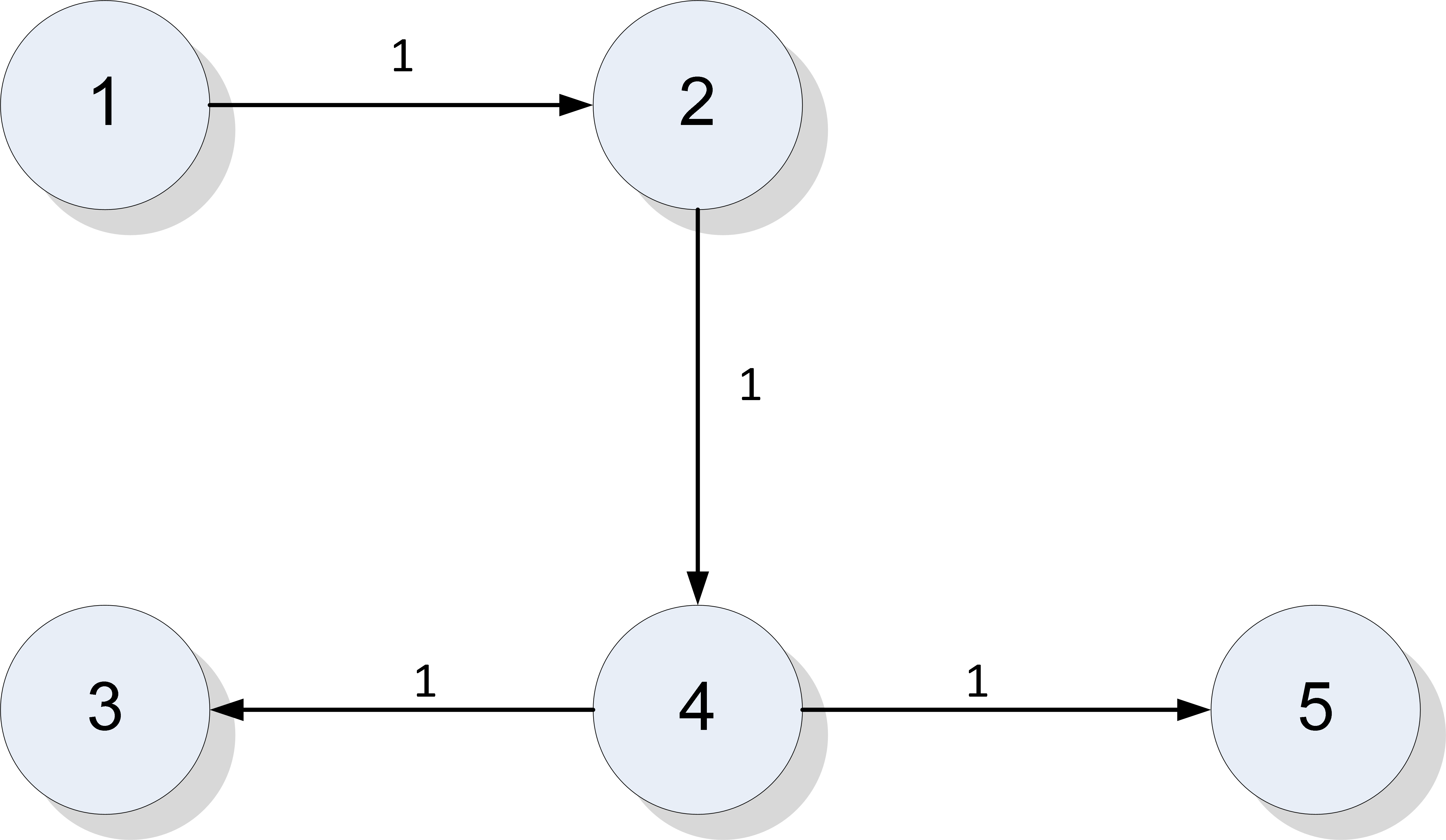
Case $1$ : Consider a MAS with $4$ agents with agent models $(C_{i},A_{i},B_{i})$ for $i\in\{1,\ldots,4\}$ , and directed communication topology shown in Figure 3.
$\bullet$

Case $2$ : In this case, we consider a MAS with $3$ agents with agent models $(C_{i},A_{i},B_{i})$ for $i\in\{1,\ldots,3\}$ and directed communication topology shown in Figure 4.
$\bullet$

Case $3$ : Finally, we consider a MAS with $5$ agents with agent models $(C_{i},A_{i},B_{i})$ for $i\in\{1,\ldots,5\}$ and directed communication topology shown in Figure 5.

Figures 6-8 show that output synchronization is achieved for all three cases. The simulation results also confirm that the protocol design is independent of the communication graph and is scale-free so that we can achieve output synchronization with one-shot protocol design, for any graph with any number of agents.

References

[1] H. Bai, M. Arcak, and J. Wen. Cooperative control design: a systematic, passivity-based approach. Communications and Control Engineering. Springer Verlag, 2011.
[2] Z. Chen. Feedforward design for output synchronization of nonlinear heterogeneous systems with output communication. Automatica, 104:126–133, 2019.
[3] C. Godsil and G. Royle. Algebraic graph theory, volume 207 of Graduate Texts in Mathematics. Springer-Verlag, New York, 2001.
[4] H.F. Grip, A. Saberi, and A.A. Stoorvogel. On the existence of virtual exosystems for synchronized linear networks. Automatica, 49(10):3145–3148, 2013.
[5] H.F. Grip, A. Saberi, and A.A. Stoorvogel. Synchronization in networks of minimum-phase, non-introspective agents without exchange of controller states: homogeneous, heterogeneous, and nonlinear. Automatica, 54:246–255, 2015.
[6] H.F. Grip, T. Yang, A. Saberi, and A.A. Stoorvogel. Output synchronization for heterogeneous networks of non-introspective agents. Automatica, 48(10):2444–2453, 2012.
[7] H. Kim, H. Shim, and J.H. Seo. Output consensus of heterogeneous uncertain linear multi-agent systems. IEEE Trans. Aut. Contr., 56(1):200–206, 2011.
[8] X. Li, Y. C. Soh, L. Xie, and F. L. Lewis. Cooperative output regulation of heterogeneous linear multi-agent networks via ${H}_{\infty}$ performance allocation. IEEE Trans. Aut. Contr., 64(2):683–696, 2019.
[9] Z. Li, Z. Duan, G. Chen, and L. Huang. Consensus of multi-agent systems and synchronization of complex networks: A unified viewpoint. IEEE Trans. Circ. & Syst.-I Regular papers, 57(1):213–224, 2010.
[10] M. Mesbahi and M. Egerstedt. Graph theoretic methods in multiagent networks. Princeton University Press, Princeton, 2010.
[11] H. Modares, F.L. Lewis, W. Kang, and A. Davoudi. Optimal synchronization of heterogeneous nonlinear systems with unknown dynamics. IEEE Trans. Aut. Contr., 63(1):117–131, 2018.
[12] R. Olfati-Saber, J.A. Fax, and R.M. Murray. Consensus and cooperation in networked multi-agent systems. Proc. of the IEEE, 95(1):215–233, 2007.
[13] R. Olfati-Saber and R.M. Murray. Agreement problems in networks with direct graphs and switching topology. In Proc. 42nd CDC, pages 4126–4132, Maui, Hawaii, 2003.
[14] R. Olfati-Saber and R.M. Murray. Consensus problems in networks of agents with switching topology and time-delays. IEEE Trans. Aut. Contr., 49(9):1520–1533, 2004.
[15] A.Y. Pogromsky, G. Santoboni, and H. Nijmeijer. Partial synchronization: from symmetry towards stability. Physica D, 172(1-4):65–87, 2002.
[16] Y. Qian, L. Liu, and G. Feng. Output consensus of heterogeneous linear multi-agent systems with adaptive event-triggered control. IEEE Trans. Aut. Contr., 64(6):2606–2613, 2019.
[17] W. Ren and E. Atkins. Distributed multi-vehicle coordinate control via local information. Int. J. Robust & Nonlinear Control, 17(10-11):1002–1033, 2007.
[18] W. Ren, R.W. Beard, and E. Atkins. Information consensus in multivehicle cooperative control. IEEE Control Systems Magazine, 27(2):71–82, 2007.
[19] W. Ren and Y.C. Cao. Distributed coordination of multi-agent networks. Communications and Control Engineering. Springer-Verlag, London, 2011.
[20] S.E. Tuna. LQR-based coupling gain for synchronization of linear systems. Available: arXiv:0801.3390v1, 2008.
[21] S.E. Tuna. Synchronizing linear systems via partial-state coupling. Automatica, 44(8):2179–2184, 2008.
[22] S.E. Tuna. Conditions for synchronizability in arrays of coupled linear systems. IEEE Trans. Aut. Contr., 55(10):2416–2420, 2009.
[23] P. Wieland, R. Sepulchre, and F. Allgöwer. An internal model principle is necessary and sufficient for linear output synchronization. Automatica, 47(5):1068–1074, 2011.
[24] C.W. Wu. Synchronization in complex networks of nonlinear dynamical systems. World Scientific Publishing Company, Singapore, 2007.
[25] T. Yang, A. Saberi, A.A. Stoorvogel, and H.F. Grip. Output synchronization for heterogeneous networks of introspective right-invertible agents. Int. J. Robust & Nonlinear Control, 24(13):1821–1844, 2014.
[26] M. Zhang, A. Saberi, and A.A. Stoorvogel. Synchronization in a network of identical continuous- or discrete-time agents with unknown nonuniform constant input delay. Int. J. Robust & Nonlinear Control, 28(13):3959–3973, 2018.