Vacuum Stability Conditions for Higgs Potentials with Triplets
Abstract
Tree-level dynamical stability of scalar field potentials in renormalizable theories can in principle be expressed in terms of positivity conditions on quartic polynomial structures. However, these conditions cannot always be cast in a fully analytical resolved form, involving only the couplings and being valid for all field directions. In this paper we consider such forms in three physically motivated models involving triplet scalar fields: the Type-II seesaw model, the Georgi-Machacek model, and a generalized two-triplet model. A detailed analysis of the latter model allows to establish the full set of necessary and sufficient boundedness from below conditions. These can serve as a guide, together with unitarity and vacuum structure constraints, for consistent phenomenological (tree-level) studies. They also provide a seed for improved loop-level conditions, and encompass in particular the leading ones for the more specific Georgi-Machacek case. Incidentally, we present complete proofs of various properties and also derive general positivity conditions on quartic polynomials that are equivalent but much simpler than the ones used in the literature.
I Introduction
Since the experimental discovery of a Standard Model (SM)-like Higgs particle at the LHC Aad:2012tfa; Chatrchyan:2012ufa and the lack so far of any direct evidence for physics beyond the standard model (BSM)11 1 possible indirect ”evidence” notwithstanding Pich:2019pzg, one might ask whether the properties of the discovered GeV scalar particle being so much close to the SM predictions (see e.g. ExpHiggsLHC) leaves any room for BSM physics to reside below the TeV or at the nearby few TeV scale. If new physics is present in the electroweak symmetry breaking sector it should either be very heavy (almost decoupled) or light but having very weak mixing with the SM-Higgs. For the latter case, extensions of the scalar sector of the SM by complex or real triplets, or further extensions comprising Left-Right symmetric gauge groups, or possibly higher representation multiplets, are appealing possibilities. A typical example is the Type-II seesaw model for neutrino masses Konetschny:1977bn; Cheng:1980qt; Lazarides:1980nt; Schechter:1980gr; Mohapatra:1979ia; Mohapatra:1980yp, for which an essentially SM-like physical Higgs state is unavoidable, a consequence of the very small mixing between the doublet and triplet neutral components being set off by the tiny (Majorana) neutrino mass scale as compared to the electroweak scale. Another example is the Georgi-Machacek model Georgi:1985nv; Chanowitz:1985ug with one complex and one real triplet such that a tree-level custodial symmetry is preserved in the scalar sector through a global .
These scenarios have triggered various activities both on the phenomenological level, (including left-right symmetric or not, supersymmetric or not, scenarios) see e.g. among the recent works Gluza:2020qrt; Padhan:2019jlc; Primulando:2019evb; Fuks:2019clu; Ghosh:2017pxl; Ouazghour:2018mld; Ait-Ouazghour:2020slc; Dev:2013ff; Dev:2017ouk; Dev:2018kpa; Dev:2019hev; Frank:2020mqh; Huitu:2020qxm (and references therein), and in experimental searches at the LHC for neutral, charged, and in particular doubly-charged scalar states that are specific to such class of models decaying either to same-sign leptons or boson pairs Aaboud:2017qph; ATLAS:2020ius, Chatrchyan:2012ya; CMS:2017pet. As for any extension of the SM, and in the absence of a unifying ultraviolet completion, these models have an increased number of free parameters and thus a large freedom in particular for the physical spectrum of the scalar sector. Theoretical conditions such as the stability of the potential, a consistent electroweak vacuum, unitarity bounds, etc., are thus welcome as a guide together with the experimental exclusion limits to narrow down future search strategies.
The present paper focuses on the potential stability issue for three models: the Type-II seesaw model, the Georgi-Machacek model, and a generalized two-triplet model. The aim is to address as thoroughly as possible the theoretical determination of necessary and sufficient (NAS) conditions on the scalar couplings that ensure a physically sound bounded from below (BFB) potential. The NAS BFB conditions have already been considered in the corresponding literature. Inspired by the approach of ElKaffas:2006nt initially proposed for the general two-Higgs doublet potential, the strategy consists in a change of parameterization of the field space reducing it to a minimal set of variables corresponding to positive-valued ratios of field magnitudes and to field orientations varying in compact domains. It is then found that in contrast with the general two-Higgs doublet case, the general doublet-triplet potential leads to a simplification that allows a fully analytical solution. A complete answer was given first in Arhrib:2011uy and Bonilla:2015eha for the Type-II seesaw model. Following the same approach the NAS BFB conditions were provided for the Georgi-Machacek model in Hartling:2014zca. We will nevertheless reexamine the issue for these two models, supplementing with complete proofs, for reasons that will become clear in the course of the study. Encouraged by the success of the approach, we extend it in the present paper to a generalized two-triplet model, that we will dub pre-custodial, for which we provide novel results by deriving the full NAS BFB conditions. Some stability constraints have already been given for this model in Blasi:2017xmc and Krauss:2017xpjcorresponding however to specific directions in the field space, thus to a subclass of necessary conditions. This pre-custodial model can be of phenomenological interest by itself, but can also serve as a guideline for the effective potential beyond tree-level in the Georgi-Machacek model.
The main issue of the analysis will be to cast the conditions in a form as close as possible to a fully resolved one. By ‘fully resolved’ we mean an analytical expression that depends solely on the couplings with no reference to orientations or magnitudes in field space. A fully resolved form, when possible, is an ideal result both technically, since no scan over the field configurations is needed, and physically, as consistency constraints are expressed directly in terms of the (physical) couplings. This was the case for the conditions derived in Arhrib:2011uy, Bonilla:2015eha while in Hartling:2014zca the conditions were resolved with respect to only one parameter, thus remaining in a partially unresolved form albeit with a residual field dependence reduced to a compact domain. As we will see, similar configurations arise in the pre-custodial model where the resolving occurs at different stages with respect to different parameters. A hindrance in the way of reaching fully resolved conditions emerges whenever dealing with a quartic polynomial that cannot be reduced to a biquadratic one. This fact motivated us to investigate further a rather mathematical question, the positivity of general quartic polynomials, for which we determine NAS conditions that are simpler than the ones found in the literature.
A word of caution is in order here: The NAS BFB conditions we are considering are obtained by requiring the tree-level potential not be unbounded from below in any direction in the field space. It is only in that sense that they are necessary and sufficient. Obviously they might be only necessary in a wider physical sense when taking into account the structure of the vacua. Moreover, going beyond tree-level would modify these conditions. As alluded to above and will be briefly discussed towards the end of the paper, the tree-level conditions can, however, encapsulate in some cases the leading loop corrections.
Several methods to treat the stability of the potential have been conceived in the literature, e.g. specifically for multi-Higgs-doublets models Maniatis:2006fs; Maniatis:2014oza; Maniatis:2015gma including elegant geometric approaches Ivanov:2006yq, or more general methods relying on copositivity Kannike:2012pe; Chakrabortty:2013mha; Kannike:2016fmd or on other powerful mathematical techniques Ivanov:2018jmz (and references therein). As attractive as it may seem, the ability of the latter systematic methods to treat in principle any model through ready-to-use packages BFBpackage, can yet in practice run into technical difficulties when dealing with extended scalar sectors as noted in Ivanov:2018jmz. Also to the best of our knowledge a model with one triplet has been treated using copositivity Chakrabortty:2013mha but for which only specific directions in field space where considered in agreement with Arhrib:2011uy, while Babu:2016gpg obtained with this method the all-directions conditons for the Type-II seesaw model in a form different from that of Arhrib:2011uy. It should however be stressed that the copositivity method cannot always be applied to potentials with extended Higgs multiplets when all -dimensional operators allowed by the gauge symmetries and renormalizability are considered. This was the case for the doublet extensions studied in Maniatis:2006fs; Maniatis:2014oza; Maniatis:2015gma, and will be the case here for the extensions with two Higgs triplets.22 2 More precisely, the potential cannot always be cast in a bilinear form involving positive-definite independent vector components and an optimal space dimension to make the method advantageous; more on this at the end of Section V. Models with increased symmetries can be more tractable, see e.g. Deshpande:1977rw, Chauhan:2019fji. Thus, the more pedestrian and somewhat mathematically lowbrow approach we adopt in this paper remains in our opinion an efficient way of tackling the stability problem specifically for the models under consideration with two triplets.
The paper is organized as follows. In Section II we revisit the derivation of the NAS-BFB conditions for the Type-II seesaw model finding equivalence with the conditions of Bonilla:2015eha that corrected Arhrib:2011uy, but stress that the conditions of Arhrib:2011uy do remain valid necessary and sufficient when one of the couplings is negative. Adding one real triplet, the approach is extended to the general pre-custodial model in Section III, including the Georgi-Machacek model as a special case. This section contains the bulk of the new results. We recall some useful ingredients of the two models potentials in Sections III.1 and III.2. In Section III.3 we first identify six field dependent variables that provide a reduced parameterization of the field space suitable for the BFB study, four of which, dubbed -parameters, vary in compact domains. We then investigate the NAS-BFB conditions following a procedure where the resolving with respect to these six field-dependent variables is performed step-by-step. Section III.4 deals with the analytical determination of the domains of variation of the -parameters as well as all 2,3,4-dimensional analytical correlations between them. In Section III.5 we derive the main results identifying the fully and partially resolved branches of the NAS-BFB conditions. The special case of the Georgi-Machacek model is reconsidered in Section III.6 where we relate the reduced parameters to those of the pre-custodial model and provide a proof of their domain of variation that was only conjectured in the literature. Section IV illustrates an unexpected feedback of the Georgi-Machacek model on the pre-custodial one. A wrap-up with further illustrations, comments and a user’s guide, is given in Section V and we conclude in Section VI. Further material and detailed proofs, either missing in the literature for known properties, or for the new results found in this paper are given in appendices A – F. Special attention is payed, in appendices G and H, to the mathematical issue of deriving simple forms for the NAS positivity conditions of quartic polynomials .
II The Type-II seesaw doublet-triplet Higgs potential
We first sketch the main ingredients, relying on the detailed analysis and notations of Arhrib:2011uy to which the reader may refer for more details.
The potential reads
denotes the standard scalar field doublet and a colorless complex triplet scalar field, with charge assignments and under ,
We have used the traceless matrix representation for the triplet and wrote the two multiplets in terms of their complex valued scalar components and indicated a choice of electric charges with the conventional electric charge assignment for the doublet and following with and for the triplet. denotes the second Pauli matrix. The potential is invariant under field transformations and where denotes an arbitrary element of in the fundamental representation. Since we are only interested in the issue of boundedness from below of the potential, we need not go further here into the details of the dynamics of spontaneous electroweak symmetry breaking, the structure of the physical Higgs states and the generation of Majorana neutrino masses.
II.1 The BFB conditions
In order to cope generically with the shape of along all possible directions of the -dimensional field space, we adopt a reduced parameterization for the fields that will turn out to be particularly convenient to entirely solve the problem analytically. Following Arhrib:2011uy we define:
| (7) | |||||
| (8) | |||||
| (9) | |||||
| (10) | |||||
| (11) |
Obviously, when and scan all the field space, the radius scans the domain and the angle . With this parameterization it is straightforward to cast the quartic part of the potential, denoted hereafter by and given by the second line of Eq. (), in the following simple form,
| (12) |
We stress here that the crux of the matter is the existence of a parameterization, Eqs (7 -11), which allows to scan all the field space and in the same time recasting the relevant part of the potential into a biquadratic form in . It is the concomitance of these two facts that allows a tractable and complete analytical solution for the necessary and sufficient boundedness from below conditions. Indeed, the absence of linear and/or cubic powers of in Eq. (12) is anything but generic. (For instance, in a similar parameterization initially proposed in ElKaffas:2006nt to study two-Higgs-doublet models such terms do remain, hindering an easy fully analytical treatment.)
One can thus consider only the range in accordance with the above stated range for . Boundedness from below is then equivalent to requiring for all and all in their allowed domain. The -free necessary and sufficient conditions on the ’s have already been given in Arhrib:2011uy33 3 We use the conventional notations and for the Boolean operators ’AND’, ’OR’ and ’NOT’, respectively.:
| (13) |
Note that the second inequality above is non-strict. This accounts rigorously for the only possible equality among the NAS conditions that is compatible with requiring to be strictly positive.44 4 In Section III.3 we will elaborate further on the meaning of the condition , as well as on the fact that the parameter varies independently of and . These inequalities are a subset of the general necessary and sufficient (NAS) positivity conditions for a quartic polynomial (see Appendix G). We stress here that Eq. (13) answers fully the question of (tree-level) boundedness from below in the totality of the -dimensional field space. There remains however the dependence on and that parameterize the relative magnitudes of the dimension four gauge invariant operators in Eq. () that are not controlled solely by and .
In Arhrib:2011uy the authors relied on this allowed range and on the monotonic dependence on in Eq.(13) to obtain equations (4.21),(4.22) and (4.23) of Arhrib:2011uy reproduced in Appendix B.0.2 for later discussions. The authors of Bonilla:2015eha rightly observed that Arhrib:2011uy had actually overlooked the fact that being correlated, cannot reach an arbitrary point in the rectangle defined by Eq.(14). Starting from Eq. (13) and using the constraint
| (15) |
they showed that the set of conditions Eqs. (190 - 192) established in Arhrib:2011uy, although sufficient in all field space directions, are in fact not necessary, even though deviation from absolute necessity is typically at the few percent level. Although we totally agree with their general observation, we will see that despite the correlation between and the conditions Eqs. (190 - 192) do remain sufficient and necessary whenever ; the modification will come only for . We will come back to this point in more detail later on in Appendix B.
For now, we just add that, as shown in Appendix A.0.3, it is possible to cast the and parameters as follows
| (16) | |||||
| (17) |
with two independent cosines taking any value in their allowed domain ; note also that Eq. (15) comes as a direct consequence of these equations.
Altough the authors of Bonilla:2015eha wrote a correct form of the necessary and sufficient BFB conditions, they only sketched a proof of their result. In Appendix B, we provide a detailed proof through a careful study of Eq. (13) leading to an alternative form of the fully resolved NAS BFB conditions. The latter reduce to:
| (18) |
where
| (19) | |||
| (20) | |||
| and | |||
| (21) |
Note also that Eq. (21) implies and so that the part is relevant only when these conditions are satisfied simultaneously.
The above constraints are in fact totally equivalent to Bonilla:2015eha although they have a slightly different form. Indeed the equivalence is not straightforward as the two involved Boolean forms are in general not equivalent to each other. However, they become equivalent due to the implication given by Eq. (189). The above constraints:
- •
constitute an independent check of the results of Bonilla:2015eha.
- •
- •
- •
III Generalization adding one extra real triplet
Such a generalization can be of phenomenological interest by itself, but is also motivated by the structure of the Georgi-Machacek model beyond the tree-level Gunion:1990dt.
III.1 The pre-custodial potential
Defining
with a different notation for the complex triplet , and as defined in Eq. (II), a real triplet ( real-valued), we write the most general renormalizable pre-custodial potential involving and as follows,
| (27) |
where the dimension-, - operators are collected in
| (28) | |||||
and the dimension- operators in
| (29) | |||||
is invariant under field transformations
| (30) | |||||
where denotes an arbitrary element of in the fundamental representation. This potential was written in Gunion:1990dt and later on in Blasi:2017xmc with which we agree up to different normalizations and notations55 5 with the field correspondence as given by Eq. (III.2) and couplings correspondence: , , , , , and . Note that our normalization factors for the various couplings are chosen such that they cancel out for at least one vertex originating from each operator when symmetry factors are taken into account in the Feynman rules.. All other dimension-,- gauge invariant operators are either vanishing or can be expressed in terms of the ones listed above. (For completeness we give a proof of this in Appendix C.)
III.2 The Georgi-Machacek potential
This model Georgi:1985nv; Chanowitz:1985ug, a special setup of the model presented in the previous subsection, allows to extend the validity of the SM tree-level (approximate) custodial symmetry in the presence of triplet scalar fields. In particular the potential reads
| (31) |
| (32) | |||||
| (33) | |||||
where we followed the notations of Hartling:2014zca.66 6 In Eqs. (32, 33) with the Pauli matrices are the usual generators in the fundamental representation, the generators in the triplet (adjoint) representation, with , and some rotation matrix about which we skip here the details (see Aoki:2007ah and Hartling:2014zca) as Eq. (32) will not be relevant to our study. We hat the ’s to distinguish them from those of Sec. II, and define the scalar bi-doublet and bi-triplet as
so that the normalization of the VEVs are the same as in Hartling:2014zca. Note also the sign difference in and between Eq. (III.1) and Eq. (III.2). The potential is then mapped onto through the following correspondence among the couplings
| (45) |
provided, however, the following correlations hold for the pre-custodial potential couplings:
| (46) | ||||
The potential enjoys an increased symmetry as compared to that of , Eq. (30), with an invariance under an extra global ,
| (47) | |||
| (48) |
where denotes -dimensional representation of . The correlations given by Eq. (46) can thus be viewed as encoding the tree-level constraints imposed by the global symmetry on the potential. We come back to this point in Sec. V when discussing briefly quantum effects. References Gunion:1990dt, Blasi:2017xmc considered such correlations.77 7 We agree with Blasi:2017xmc except for a factor two difference on the right-hand side of the first equation of the second line of Eq. (46) as compared to the first equation of the second line of Eq. (10) of Blasi:2017xmc.
III.3 The pre-custodial BFB conditions
Being a polynomial in the fields, the tree-level potential has no singularities at finite values of the fields; it follows that boundedness from below means that the potential does not become infinitely negative at infinitely large field values. This is equivalent to requiring strict positivity of the quartic part of the potential, Eq. (29), for all field values in all field directions. The latter requirement is sufficient as it implies that at infinitely large field values, where in Eq. (27), the potential does not become infinitely negative. That it is also necessary might not seem obvious since the last term in Eq. (29) is linear in and in , so that might be negative for some finite values of the fields without being unbounded from below. That this does not happen, and the above requirement is indeed necessary, can be easily seen as follows: If there existed a point in field space where , then scaling all the fields at that point by the same real-valued amount would have lead to , implying unboundedness from below since can be chosen infinitely large. Note finally that strict positivity is important here because a vanishing at very large field values would generically lead to the dominance of which, barring accidental cancellations in some field directions, always possesses unbounded from below directions!
The BFB conditions are thus the necessary and sufficient conditions on the nine couplings of Eq. (29) that ensure
| (49) |
Of course, loop corrections will modify the conditions on the couplings resulting from Eq. (49), although the effects can be partly encoded in the runnings of the couplings through a renormalization group improvement of the potential. (We will come back briefly to this point in Section V.) Note also that the above definition of boundedness from below does not take into account the actual pattern of spontaneous symmetry breaking that would typically lead to more stringent constraints.
The condition in Eq. (49) should be verified in the full -dimensional space of the real-valued field components of the and multiplets. However, symmetries of the model (and possibly accidental symmetries akin to ) will help reduce the number of relevant degrees of freedom. Starting from Eq. (29) we generalize the parameterization of Eqs. (7 - 11) using spherical-like coordinates as follows:
| (50) | |||||
| (51) | |||||
| (52) | |||||
| (53) |
where is a non negative number, and and two angles. It will also prove useful to define the following real-valued quantities,
| (54) | |||
| (55) | |||
| (56) |
Hereafter we will refer to the latter four parameters as the -parameters. In terms of and the -parameters, the quartic part of the potential now reads
| (57) |
where
| (58) | ||||
It becomes evident from Eqs. (57–58) that the positivity of does not depend explicitly on all ten terms of the right-hand side of Eq. (29), but just on the reduced set of the six combinations of gauge invariant operators defined in Eqs. (54 – 56). The sought-after NAS BFB conditions on the ’s are thus those that ensure
| (59) |
It is important to note that scanning independently over all values of the thirteen real-valued components of the fields and amounts to varying and the -parameters. The latter, however, do not all vary independently. For one thing, the -parameters vary in bounded domains: and are nothing but respectively and defined in Eqs. (10, 11). Hence
| (60) | |||||
| (61) |
as shown in appendix A. Furthermore, one can show that
| (62) | |||||
| (63) |
see Appendix D for details. For another, the -parameters are uncorrelated only locally. But similarly to what was pointed out in Bonilla:2015eha and discussed at length in sec. II.1 for the Type-II seesaw model potential, they are correlated globally in that they cannot reach the boundaries of their respective domains independently of each other. The actual domain in the -dimensional -parameters space is certainly not the simple hyper-cube defined by Eqs. (60 –63). One can approach the true domain by considering the projected domains on the sub-spaces of these parameters taken two-by-two. This is not trivial to establish and will be carried out in full details in Sec. III.4. The more difficult task of determining fully the true domain will be discussed in Section III.4.7.
In contrast, the variables and vary in independently of each other and of the -parameters. In essence, the -parameters being ratios of different gauge invariant combinations of the fields can be seen as functions of cosines and sines of angles defined separately in the , and field spaces, where and represent lengths. This hints at the obstruction to span the full hyper-cube as noted above. Whereas and , being two ratios of these three lengths, are clearly independent of each other and of the -parameters. It follows that can be varied independently from and in Eq. (59) Consequently, the NAS conditions for the strict positivity of , , are those of a biquadratic polynomial in , namely conditions on the ’s satisfying
| (64) |
As noted previously, only the highest degree monomial coefficient can vanish. However, for the sake of simplicity we will consider in the sequel only the strict inequality . It is convenient to recast the above inequalities in the following equivalent form that disposes of the (less tractable) square root:
| (65) | |||
which simplifies further to
| (66) | |||
| (67) | |||
III.3.1 :
We consider first the conditions in Eqs. (66) as they are common to the union of the two conditions of Eqs. (67). The coefficient being itself biquadratic in and the latter independent of the -parameters, see Eq. (58), the corresponding NAS positivity condition is in turn of the same form as Eqs. (66, 67). The two inequalities in Eq. (66) are thus equivalent to:
| (68) | |||||
| (69) | |||||
Note that the second inequality in Eq. (68) and the first inequality in Eq. (69) depend solely on or on . They can be easily resolved since the dependence on these parameters is monotonic; if required to be valid in the domains given by Eqs. (60, 62), they become equivalent to requiring them simultaneously at the two edges of these domains, namely:
| (70) |
for the first, and
| (71) |
for the second. Equation (69)-(II) needs more care due to the nontrivial global correlation between and (see next section and Fig. 2), and will be kept in its present form for the time being. One will also have to tackle a further complication involving the two inequalities of Eq. (69). Indeed, due to the ‘or’ structure of Eq. (69), none of the two corresponding inequalities need to be necessarily valid for all in their domains; it suffices that one of the two inequalities be satisfied in a given subset of , and the other inequality satisfied in the complementary subset. In particular, Eq. (71) is only sufficient. To reach the NAS conditions one will have to consider all possible coverings of the domain by two subsets for which such a configuration holds. This issue will be solved explicitly in Sec. III.5.1.
III.3.2 :
We turn now to the two inequalities of Eq. (67). The first is quadratic in , see Eq. (58), but could in principle be treated as a biquadratic polynomial in , since . The second, , is a general quartic polynomial in this same variable. This is the first place where we encounter the issue of positivity conditions for a general quartic polynomial. Relying on a classic theorem about single variable polynomials that are positive on , we derive in Appendix G a relatively tractable form of the corresponding NAS conditions for a quartic polynomial. However these conditions are not directly applicable to the case at hand since the relevant variable here, , is in . In this case the NAS conditions would obviously be less restrictive, see for instance Powers:2000; Benoist:2017 for recent reviews.88 8 Somewhat surprisingly, corresponding theorems, when the variable does not span the full interval, seem not to have been referenced in the mathematics literature before the 1970’s, see Polya:1976. Relying on these theorems we extend the results of Appendix G to the domain in Appendix H.
However, this is not the full story. Similarly to what we stated above in subsection III.3.1 regarding Eq. (69), the ‘or’ structure of Eq. (67) implies that it is sufficient for the two inequalities and to be separately valid in two complementary subsets of the allowed and -parameters domains. The NAS conditions will then be obtained by investigating all possible coverings of these domains for which this happens. The upshot is that the possibility of varying freely with respect to the -parameters is not sufficient anymore. Indeed, a given subset of the -parameters where for instance (or ) will be necessarily correlated with . A strategy for an explicit resolution will be given in Sec.III.5.2.
Although it will prove unavoidable to deal with positivity conditions of quartic polynomials on sub-domains of , it will still be useful for the subsequent discussions to replace from the onset by a variable on if possible. This is indeed the case if one considers the variable defined as
| (72) |
since can take either signs, cf. Eq. (63). However, in order to apply safely the NAS positivity conditions on a polynomial in , one should make sure that is not correlated with the other parameters, and appearing in the inequalities, even though these parameters are globally correlated with .
It is obviously the case for since is uncorrelated with the other parameters and allows to scan independently of the value of the full range. However, the sign of is controlled by which is globally correlated with and . It is thus crucial to check that the sign of is not correlated with the latter parameters. That this is indeed the case is easily seen by recalling that all the inequalities are required to be valid in the field space, and noting that and remain unchanged, while flips sign, at the two field space points and (or equivalently at and , or and ), see Eqs. (55, 56). It follows that one can change freely the sign of for any given configuration of and . (As we will see in the next subsection, Figs. (3 - 5), this translates into domains symmetrical around .) The variable is thus genuinely uncorrelated with the other field dependent reduced parameters.
III.4 Global correlations among the -parameters
In this section we first determine the allowed domains of the -parameters taken two by two, then combine the resulting six global correlations to obtain an analytical approximation of the full D domain. Since the -parameters are ratios of gauge invariant quantities, cf. Eqs. (55,56), it is convenient to choose a gauge that reduces the dependence on the set of components fields of the , and multiplets. Apart from the treatment of versus , we carry all the discussion in this section assuming a gauge that diagonalizes the (hermitian and traceless) multiplet as defined in Eq. (III.1), which then takes the form
It follows that the dependence on cancels out in and, up to a global sign, in .
III.4.1 versus
These parameters are identical respectively to and that were defined and studied in detail in Section II.1 and Appendix A.0.3. We just recall here the corresponding domain:
| (76) | |||||
| (77) |
illustrated in Fig. 1.
III.4.2 versus
With no particular gauge choice but using the fact that the parameter is a ratio, one can recast it in terms of reduced parameters in the following form:
| (78) |
where we defined
| (79) | ||||
with
| (80) |
Furthermore, choosing a gauge for which Eq. (III.4) is valid the parameter takes the very simple form,
| (81) |
Equations (78, 81) lead straightforwardly to
| (82) |
To determine the boundary of the allowed domain one can for instance study the variation of in Eq. (82) as a quadratic function of in the domain to identify the set of maximal and minimal possible values of for a given depending on . The maximum is reached for which lies in the allowed domain only if and . Otherwise, the maximum is reached at one of the boundary values or . We find that the boundary of the domain is given by the following four curves:
| (83) | ||||
see also Fig. 2.


III.4.3 versus
Similarly to the preceding case, we recast and in terms of reduced parameters and in the gauge where Eq. (III.4) holds:
| (85) |
where and are as previously defined and
| (86) | ||||
with and . (Note that (modulo ).)
A numerical parametric scan over the various angles allows to guess the boundary of the versus domain. The result turns out to be very simple given by the two curves:
| (87) | |||||
| (88) |
illustrated in Fig. 3. The proof for the upper boundary (87) is simple: It suffices to exhibit particular configurations of the various angles for which saturates its upper bound while scans all its allowed domain. An example is , keeping all the ’s free. This gives and , which proves the above statement. The lower boundary (88) is much more difficult to establish analytically. The proof is somewhat involved and will be relegated to Appendix D.0.3.
III.4.4 versus
Here again a numerical parametric scan over the various angles helps guessing the boundary of the versus domain. However, one still needs for that to admit ad hoc that the whole boundary is obtained when . The analytical proof is quite involved and is given in Appendix D.0.4 for completeness. We find that the boundary is determined by the following:
| (89) | ||||
III.4.5 versus
From Eqs. (81,85,80,63), one obtains readily
| (90) |
where (defined in Eq. (240)) and vary independently in the domain . It is then clear that for each given value of , reaches its maximal value compatible with Eq. (90) when . Also the minimal value is reached for any value of . The boundary of the allowed domain in the plane versus is thus delimited by the two curves:
| (91) | |||||
| (92) |
as shown on Fig. 5.
III.4.6 versus
The boundary of the allowed domain in the plane is given by:
| (93) | |||||
| (94) | |||||
| (95) | |||||
| (96) |
see Fig. (6). The proof strategy is similar to the one in Sec. (III.4.2) albeit somewhat more involved, the convenient variable here to study the variation of being . (See Appendix D.0.5 for details.)
III.4.7 The D -potatoid
The D projections of the -parameters domain determined analytically in the previous subsections will allow, in some cases, a fully analytical resolving of the BFB conditions on the ’s. Obviously generalizing beyond D along the same lines becomes non-tractable analytically. In principle one can then proceed numerically, scanning over part or all of the seven angles entering Eqs. (78, 81, , 85), to determine the D projections as well as the true D allowed domain of the -parameters. However, this would cut short the possibility of further analytical resolving for the conditions on the ’s.
We will proceed differently here by constructing an analytical approximation of the true -parameters domain from a back-projection using only six planes. Obviously any point in the true domain should have its projections on the six planes lying within the six domains determined above. This necessary condition can be characterized by the interior of a four dimensional convex domain that we will refer to as the D potatoid. To determine explicitly this D potatoid we first express separately in the form of a logical (inclusive) disjunction each of the six domains of Figs. 1– 6, then form the logical conjunction of these disjunctions. The resulting Boolean expression is somewhat involved but, interestingly enough, it eventually simplifies to the following form:
| (97) | |||
This form is non-trivial in that it does not display explicitly all six correlations among the four -parameters; in particular, the correlation between and does not appear explicitly and, depending on , either only three or five of the six correlations are explicitly needed. These features will prove useful when resolving the constraints in Section III.5.2. It is also informative to partially visualize the D potatoid by considering its D projections along each of the four directions. This amounts to combining the domains three by three which leads after some simplifications to:
| (102) |
Figure 7 shows these D projections. It is easy to check by eye from this figure that further projection on the various planes reproduces the domains shown in Figs. 1– 6. However, the rounded (and even non-smooth) edges featured in Fig. 7 hint at the fact that looking at projections is necessary but not sufficient to determine the true D domain of the - parameters. For instance a point lying just outside the chopped edge in Fig. 7 (a), that is a point excluded for sure, would still project on the interior of the domains of Figs. 3,5,6. Obviously this is not yet fully a counter example as the considered point might still project outside one of the three remaining D domains. But on general grounds the potatoid determined by Eq.(97), even though enclosing the true D domain, is not necessarily identical to it. Since relying on continuity arguments one does not expect holes in the interior of the true domain, that would leave no imprint in the projections on the six planes, one concludes that differences between the potatoid and the true domain should be located on the boundaries of the former. We defer a detailed study showing that this is indeed the case till section IV. There we will make use of an interesting feedback on the issue from the more constrained Georgi-Machacek model.



III.5 Resolved forms of the pre-custodial BFB conditions
For now we ignore the above subtleties and exploit in the present section the domains of the - parameters, as determined so far, to push as much as possible an explicit resolving of the conditions given by Eqs. (66, 67) for the parameters themselves.
III.5.1 Resolving
Resolving conditions (66) with respect to , they become equivalent to Eqs. (68, 69). As stressed at the end of Section III.3.1, in order to fulfill the ’or’ structure of Eq. (69) one should in principle consider all possible partitions into subsets of the domain depicted in Fig. 2. Since obviously the two inequalities could be simultaneously satisfied in some parts of the domain, the subsets should be allowed to overlap. So, strictly speaking, we should consider coverings rather than partitions. More precisely:
The task can seem daunting since there are a priori infinitely many ways of forming a covering of the domain. However, one can identify a clear procedure. Note first the obvious fact that, for a given in the –space, each of the two inequalities in Eq. (69) defines separately natural partitions of the domain, namely partitions formed by a collection made of subsets where the inequality is satisfied and subsets where it is not. Moreover, among all these natural partitions, one can show that a minimal partition, made of the smallest possible number of subsets, is actually unique and made of at most two subsets.99 9 This is an immediate consequence of the binary ”yes/no” characterization of the subsets of the natural partitions defined above. Indeed, starting from a given natural partition and taking the union of all the ”yes” subsets and the union of all the ”no” subsets forms two subsets (including possibly an empty one) defining a minimal partition. The uniqueness proof then follows easily: if and are two minimal partitions, then at least one set and one set should have a non-empty intersection , since the partitions cover the same domain. This implies the whole of and to have the same ”yes/no” characterization. But this contradicts the fact that the complementary of has by definition the opposite characterization, unless . The two remaining subsets should thus be identical too, whence the uniqueness of the minimal partition. A clear strategy follows: For each given point in the –space, determine the two minimal partitions defined respectively by Eq. (69)-(I) and Eq. (69)-(II), call them and ; then check whether their union forms a covering that satisfies the required property stated above in italics, that is check whether
| (113) |
to select or reject the considered point in –space.
Given the linear dependence on in Eq. (69)-(I), the associated minimal partitioning corresponds simply to cutting the domain into regions by a straight line going vertically across the domain, at , as illustrated by the dashed line in Fig. 2. The inequality (69)-(I) is then true for any in an entire interval of the form or , and false on their respective complement. This corresponds respectively to the two minimal partitions where the ”yes” assignment holds for the right side or the left side region. Moreover, since lives in , the minimal partition reduces trivially to either or if . It is thus convenient to consider separately the NAS conditions on and that correspond to each of these four configurations of the minimal partition. These NAS conditions are easy to write down given the monotonic dependence on in Eq. (69)-(I). They are given in Fig. 8 with the labels (i), (ii), (iii) and (iv). Note that (i) and (iv) correspond to the two extreme configurations, respectively , cf. Eq. (71), and , while (ii) and (iii) are the two intermediate generic partitions.
On the other hand, as can be easily seen from the dependence on in Eq. (69)-(II), the corresponding minimal partitions are determined by convex parabolae in the plane, illustrated by the black curves in Fig. 2. The middle and bottom figures in Fig. 2 show several possible configurations when . The middle-left illustrates a generic case where Eq. (113) can never be satisfied irrespective of the ”yes/no” configurations. The middle-right and bottom-left figures, and more generally when the solid and dashed lines do not cross, illustrate the necessary configurations to allow for Eq. (113), yet one still needs to examine the ”yes/no” configurations for sufficiency. Finally the bottom-right figure where the two branches of the parabola cut through the domain, is another configuration for which Eq. (113) is impossible. Finally, when , not represented on Fig. 2, the entire domain is contained either in the non-empty subset of or in the non-empty subset of . In the latter case it is required to be entirely contained in the ”yes” region determined by the parabola.
Putting everything together, the problem becomes equivalent to solving for the following complementary conditions:
- (i)
Eq. (69)-(I) valid , partition
- (ii)
,
Eq. (69)-(I) valid only ,
Eq. (69)-(II) should be valid , i.e.
- (iii)
,
Eq. (69)-(I) valid only ,
Eq. (69)-(II) should be valid , i.e.
- (iv)
Eq. (69)-(I) false , partition ,
Eq. (69)-(II) should be valid , partition
where the numbering corresponds to that of Fig. 8.
We can now derive in a fully analytical way the resolved form of Eqs. (68, 69), or equivalently of Eqs. (69, 70) in conjunction with . The NAS conditions thus obtained on the ’s have no residual dependence on and . To retrieve these NAS conditions we followed step-by-step the partitions described above and analyzed the non-monotonic dependence on in Eq. (69)-(II) when applicable.
The details are very technical and will not be described here. We give the final result in Fig. 8 where we have defined the following Boolean expressions 3:
| (114) | |||
| (115) | |||
| (116) | |||
| (117) | |||
| (118) |
In writing this final form we used occasionally the fact that to obtain compact expressions where Eqs. (70) are implicitly taken into account in Eqs. (114, 116,118).
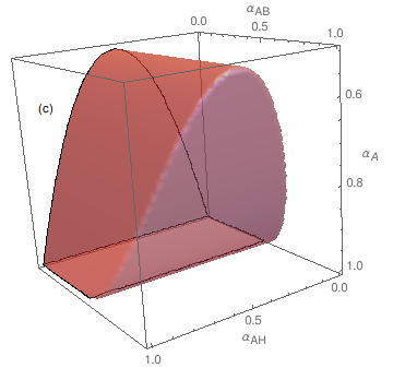
For a cross-check of our results we have performed various numerical scans simultaneously on the ’s, and on in the domain defined by Eqs. (83-I – 83-IV). This amounts to checking the validity of the conditions Eqs. (69, 70), and comparing the Boolean output with that of the resolved conditions of Fig. 8.1010 10 Throughout the paper we rely significantly on the Mathematica package Mathematica for symbolic and numerical computations as well as for the generation of the plots. One can take advantage of the fact that and are not correlated in the square to replace for this part of the domain, and without loss of information, and by their edge values in Eqs. (69)-(I), -(II). The parabola-edged part of the domain (where ), is more tricky to treat. If not sufficiently finely meshed, a numerical scan could miss some features depending on the configuration of the maximum/ minimum of the parabola. As an illustration we show in Fig. 9 the allowed D domains, for subsets of the parameters, obtained from the resolved exact conditions of Fig. 8 and compare them with the approximate ones obtained from requiring Eqs. (69, 70) to hold for just three sets of benchmark values of and lying on the boundary of their allowed domain. As expected, one of the benchmark sets leads to an approximate domain that is much less restrictive (the pink colored regions in Figs. 9 (a), (c)) than the exact domain shown in Figs. 9 (b), (d)). However, one finds that the other benchmark set (the brown colored regions in Figs. 9 (a), (c)) leads unexpectedly to an extremely good approximation of the exact domain. Obviously this accidental agreement could not have been guessed without the comparison and is not by itself a cross-check of the validity of the conditions given in Fig. 8 & Eqs (114 –118). For that we have performed large scans, points on a regular grid in the -space in the configurations of Fig. 9, or fixing only and taking points in the -space with much larger number of benchmark points, benchmark points within, or benchmark points on, the boundary of the domain. Counting the hits where the Boolean values of the approximate and exact conditions are equal or different we found in all cases a difference of less than between the approximate and exact conditions. Another significant feature of the check is that the Boolean yield of the difference is found in of the cases to be ”approximate=True, exact=False”. Only one hit with the reverse configuration would have meant the exact conditions are wrong!
In summary, we have derived the NAS conditions for in a fully analytical resolved form. They are thus necessary for the BFB of the general potential given by Eqs. (27 – 29), and can be safely applied irrespective of the , and field configurations.1111 11 Note that an alternative approach to obtain these results is to start from the third inequality in Eq. (64) with no ’OR’ structure rather than from Eq. (67). Its advantage is to avoid the use of partitions and coverings but necessitates the study of functions with square roots as in Appendix B leading though to more compact conditions. We have checked the agreement of the two approaches. The partitions/coverings approach we developped will nevertheless be unvoidable for the all-field-directions full analytical resolving of the pre-custodial model in the case , not treated in the present paper. Further comments on these conditions are deferred to Sections IV and V.
| (i) (ii) (iii) (iv) |


III.5.2 Partial resolving of
We investigate now Eq. (67) that should be valid in their allowed domains. (We use here the variable defined in Eq. (72) instead of , and refer the reader to Section III.3.2 for a discussion on the relevance of .) As argued repeatedly in Sections III.3.1, III.3.2 and discussed in detail in the previous subsection, the ’or’ structure in Eq. (67) implies that the validity of the inequalities should be required for all possible coverings of the space. However, the situation is more complex here than in the previous subsection, since , cf. Eq. (58), involves simultaneously all four ’s and is a complete quartic polynomial in . Given the particularly involved NAS conditions for quartic polynomials, Eqs. (332 - 335), we do not expect to resolve completely this case in an explicit form similar to that given in Fig. 8. The aim here is to proceed as far as possible towards an explicit resolving, then deal with the rest through mere numerical scans on the -parameters defined by Eq. (97), including some further refinements to be discussed in Sec. IV. To proceed let us first address the flowchart of the overall logic. This is sketched in Fig. 10, together with the following definitions:
- •
denotes the NAS conditions for to always have a constant sign,
- •
denotes the NAS conditions for to be positive when is in the interval and the -parameters satisfying Eq. (97).
The strategy underlying this flowchart is similar to the one adopted in the previous subsection (which the reader is referred to for definitions and notations), and should be clear by now. The upper left box of Fig. 10 corresponds to the –space points for which defines two trivial minimal partitions, or , corresponding respectively to and , while the lower left box corresponds to the –space points where defines a generic minimal partition . The boxes to the right indicate the Boolean structure including the minimal generic partition defined by to satisfy Eq. (113). We now investigate how far the Boolean expressions and can be resolved analytically.
| constant , |
| giving varying |
: Viewing , Eq. (58), as a quadratic polynomial in , we denote by its two roots. Thus corresponds to the NAS condition for which are not real-valued, that is to requiring the discriminant of this polynomial to be negative,
| (119) |
for all in the domain given by Eqs. (87, 88). Taking into account the correlations at the boundary of this domain one can obtain condition in a fully resolved analytical form. After some non-trivial Boolean simplifications we find,
| (120) |
Clearly then, the NAS conditions for the sufficient condition read, see Fig. 10,
| (121) |
However, as will be discussed later on in Sec. IV, the condition on the left-hand side of Eq. (120) is in fact
only sufficient to yield .
: To obtain we consider as a quartic polynomial in and thus require all the conditions given by Eqs. (332 - 335). The coefficients are straightforwardly read from the combination upon use of Eqs. (58, 72):
| (122) |
where
| (123) | ||||
We provide here explicitly the resulting first three conditions given by Eqs. (332):
| (124) | |||
| (125) | |||
| (126) |
where we defined
| (127) |
Condition (124) can be readily resolved: Being linear in , one requires it to hold simultaneously on the upper and lower boundary lines of the domain given by Eq. (77). The resulting conditions depend only on quadratically and can be studied straightforwardly taking into account Eq. (76). After several Boolean simplifications we find the following resolved form of Eq. (124), adding also Eq. (125),
| (128) | |||||
| (129) | |||||
Condition (126) appears much less amenable to a
resolved form as it involves all four -parameters
simultaneously. One can however still resolve it partially but this will not be pursued
further here.1212
12
For
instance, since it is biquadratic in with a positive definite coefficient of , a sufficient
condition is then a negative discriminant. The latter has a simple
form depending linearly on
and quadratically on .
The remaining conditions corresponding to Eqs. (333,334,335)
will be treated numerically.
: To obtain these conditions one again considers as a quartic polynomial in . However, now the positivity is not required on all and one needs to rely on the results derived in Appendix H. Since the latter hold for , we first map one-to-one the domains and on through the two changes of variable
| (130) |
respectively, with , then search for the conditions on the quartic polynomial in satisfying criterion (349). We note, however, two simplifcations due to the linear changes of variable: , the coefficient of given by Eq. (125), is the same as that of . It follows that the necessary condition Eq. (128) remains valid. On the other hand, the coefficients are modified with respect to Eq. (124) to, respectively, and given by:
| (131) |
Interestingly, one can show that when combined with Eqs. (68, 69), the necessary constraints
as dictated by the first of Eqs. (332), will always be satisfied by Eq. (131) irrespective of the values of
! Indeed, given Eq. (68),
when Eq. (69)-(I) is satisfied then follows trivially, and when Eq. (69)-(II) is satisfied
then , taken as a quadratic equation in , has no real-valued roots and thus again always positive.
: In this case a nonlinear change of variable
| (132) |
is used with before applying criterion (349). Here too a simplication occurs for and after the change of variable. Up to a global positive definite denominator, they are expressed in terms of Eq. (131):
| (133) | |||
and are thus always positive when combined with Eqs. (68, 69), as explained above.
To summarize, we have identified a subset of analytically resolved necessary conditions in the various branches of Fig. 10 flowchart. One now should combine these conditions with the other analytically resolved conditions given in Fig. 8 and Eqs. (114 - 118) and possibly also with those given by Eqs. (18 – 21). This allows a quick determination of necessary domains in the –space. Then adding the remaining necessary conditions that can be treated through numerical scans on the -parameters, one delineates the NAS BFB conditions. However, before doing so in Sec. V, we need to reexamine first the BFB conditions of the more constrained Georgi-Machacek model, as this will have some bearing on the general case.
III.6 The Georgi-Machacek BFB conditions
In Hartling:2014zca the authors provided a detailed study of the properties of the potential relying on a generalization of the parameterization used in Arhrib:2011uy. They identified the two parameters
| (134) | |||||
| (135) |
relevant to the study of the BFB conditions, writing in the form
| (136) |
with
| (137) | |||||
| (138) |
Noting that and one can relate and to the parameters defined in Eqs. (50 – 53) to obtain,
| (139) |
Then equating , Eq. (136), with , Eq. (29), and taking into account the above relations and Eqs. (45, 46), one identifies and as the coefficients of and which allows to relate them to the parameters defined in the pre-custodial case, Eqs. (54 – 56), as follows:
| (140) | |||||
| (141) |
As a cross-check of the validity of these relations, one can indeed retrieve from the fact that and the exact knowledge of the two domains given by Eqs. (83-I – 83-IV) and Eqs. (87, 88), that and as already found in Hartling:2014zca.
The allowed domain in the plane has been given in Hartling:2014zca. This was done stating that the boundary of the domain is obtained from the real valued components of the neutral field directions, that is keeping only and and zeroing all the others in Eqs. (134, 135). However, no justification was given for this statement. The aim of the present section is to provide an explicit proof for the equation of the boundary of the domain based on the symmetries of . We choose to use to rotate away the lower as well as the imaginary part of the upper components of , so that
| (142) |
(note that ref. Hartling:2014zca used instead), and use to rotate away for instance and the imaginary part of , bringing the bi-triplet X in the form
| (143) |
where denotes a real-valued scalar field.1313 13 One could be tempted to zero, on top of , the (real-valued) entry rather than . However one can show that this is not possible through a non infinitesimal rotation. More generally, one cannot zero more than two entries of through rotations. With this choice of gauge and take the following form
| (144) | |||||
| (145) | |||||
| (146) | |||||
| (147) |
where we defined the polar angles by
| (148) | |||||
| (149) | |||||
| (150) | |||||
| (151) | |||||
| (152) |
with
| (153) | |||
| (154) | |||
| (155) |
Note that due to the invariance of under one can always fix uniquely either the sign of or that of . In our parameterization while can take either signs. In Eqs. (145, 147) we kept for simplicity only linear terms in . We will come back to the exact contribution later on. Here we first concentrate on the order contributions to and , i.e. Eqs. (144, 146) which we dub and . In Appendix E we give a detailed proof for the determination of the boundary in the domain, i.e. under the working assumption that . We find that this boundary is defined by the following upper and lower curves:
| (156) |
| (157) | |||||
| (158) |
This reproduces exactly the boundary given in reference Hartling:2014zca as illustrated in Fig. 11
(note however that we deal with the inverse function with respect to reference Hartling:2014zca). As shown in Appendix E.0.3 the condition , i.e. , is sufficient and necessary for the determination of the boundary. In particular the necessity of this condition is a non-trivial result. From Eq. (144) one sees that could as well have defined a boundary. More importantly, the involved dependence on in , Eq. (146), could in principle lead to portions of the boundary with , since we are interested in the projection on the plane. (This was for instance the case for the domain studied in Sec. III.4.4.) Moreover, this is not the end of the story because the boundary defined by Eqs. (156 – 158) is obtained in the case . It remains to be seen whether would possibly enlarge the allowed domain outside this boundary. We turn now to this point. The idea is to consider a subspace of the field space for which the boundary of is reached and determine within this subspace the boundary of allowing for . As discussed above, such a subspace has necessarily , (). The bi-triplet of Eq. (143) becomes
| (159) |
One then sees from Eqs. (145, 147) that the order contributions vanish for any in this subspace, indicating that the boundary is indeed unchanged when at least if remains sufficiently small. In fact this result remains true in general beyond the first order as a consequence of an accidental symmetry: and (summation over ) are invariant under the substitution , and is invariant under the same substitution supplemented by . Thus and are invariant under these substitutions, in which case defined in Eq. (159) is replaced by
| (160) |
The key point is that the latter has the same form as given by Eq. (143) with . We are then brought back to the same configuration that leads to the fact that the boundary is reached for and is given by Eqs. (156 – 158); applied to the present case where is replaced by implies similarly that the boundary is reached for and is given by the same Eqs. (156 – 158). This completes the proof that in Eq. (143) remains within the boundary obtained for . Thus the full boundary in the plane is given by Eqs. (156 – 158):
| (161) |
In the following we will refer to this domain as the -–chips.
IV Peeling the potatoid with the chips
As already announced at the end of Sec. III.4.7, the knowledge of the exact domain of the -–chips of the Georgi-Machacek model will have a spin-off on the refinement of the D -parameters potatoid in the general pre-custodial model. That a model with an enlarged symmetry would backreact on a less symmetric and more general model is somewhat unusual. It can be understood as follows in the case at hand: The symmetry of the Georgi-Machacek model has allowed regroup the four -parameters and the parameter into just two relevant parameters and that are related to the former as given by Eqs. (140, 141). However, the equations defining the -–chips, Eqs. (161, 156 – 158), were arrived at thanks to the gauge and global symmetries, as well as to an accidental invariance of the quartic part of the Georgi-Machacek potential (see Sec. III.6 and Appendix E); in this, Eqs. (140, 141) played no role. The latter, in conjunction with Eq. (161), will thus lead to a supplementary correlation among the -parameters and that should be valid in the general pre-custodial model. It is in that sense that the Georgi-Machacek model informs about the more general model. Obviously, this information would have been redundant had we had beforehand a full knowledge of the exact D -parameters domain. This is however not the case as pointed out in Sec. III.4.7 regarding the -potatoid. Hence one can use the above information as a sufficient condition to exclude points in the -potatoid as follows: Each set of -parameters in the -potatoid defines, through Eqs. (140, 141), a unique trajectory in the plane, parameterized by . If the trajectory goes out of the -–chips then the corresponding set of -parameters values should be excluded.
We show in Figs. 12 &13 numerical scans taking into account this exclusion criterion.1414 14 In practice this is achieved by scanning over the four -parameters that satisfy Eq. (97) and following each trajectory scanning over with . Alternatively, one can use the exact -resolved form for Eqs. (140, 141), see Appendix F, and scan only on the -parameters. We used this latter alternative to cross-check our results. The red and blue dots delineate the somewhat convoluted regions of the -potatoid that are incompatible with the -–chips. As anticipated in Sec. III.4.7 and visible from the different viewing angles in Fig. 12, the excluded portions lie only at the boundary of the -potatoid. Note that the domains (shown in pink) in Figs. 12 &13 are D sections of the D -potatoid at fixed values of or or respectively; not to be confused with the D projections of the -potatoid shown on Figs. 7 (a), (b) and (d), with which it would not be possible to disentangle boundaries unambiguously. Moreover the choices of , and made in Figs. 12 &13 entail the inclusion, in the corresponding D-sections, of the full D domains Eq. (83), Fig. 2, and Eqs. (87, 88), Fig. 3, and Eqs. (76, 77), Fig. 1 respectively. These scans will thus allow to judge whether the resolved conditions on the ’s given by Fig. 8, or those given by Eq. (129) or by Eq. (120), in which the pairs of parameters , and have been eliminated respectively, are indeed necessary and sufficient or not. The answer will be yes for the first two and no for the last:
- –
One sees from Fig. 13 (a) that for there are no exclusions by the -–chips. In particular, the D section at corresponds to the full domain of Fig. 2 which is thus not reduced by the constraint from the -–chips. In fact this result could be easily retrieved once noted that the domain of Fig. 2 corresponds indeed to the D section of the -potatoid Eq. (97) at . For these values imply , cf. Eq. (140); and as seen from Fig. 11, all points remain within the -–chips . If follows that the study in Sec. III.5.1 that lead to the NAS conditions given by Fig. 8 remains valid, at least for the section. Moroever, since the domain of Fig. 2 is not only a projection but corresponds as well to the latter section of the -potatoid, then the above mentioned NAS conditions are sufficient conditions for all other sections at fixed since by construction they all fall in the interior of the domain of Fig. 2. Obviously this holds even if these sections have portions excluded by the -–chips, e.g. when as seen from Fig. 13 (a), since sufficiency is more constraining. We can thus safely conclude that the conditions given by Fig. 8 are NAS for the validity of Eq. (66) in all the -potatoid.
- –
Along a similar line of thought, one deduces from Fig. 13 (b), where there are no exclusions by the -–chips as soon as , and from the fact that the projected domain shown in Fig. 1 is also retrieved as a D section at , that the conditions given by Eq. (129) remain NAS for the validity of Eq. (124) in all the -potatoid.
- –
The case of Eq. (120) is more involved. This condition resulted from eliminating based on the full domain of Fig. 3. However, as seen from Fig. 12 (b), a portion of this domain in the range is excluded by the -–chips constraint. Equation (120) becomes thus only sufficient for the domain of Fig. 3 that corresponds furthermore to the D section at on Figs. 12 (a)–(d). It is thus also only sufficient for the full -potatoid, again because the domain of Fig. 3 is the largest section. Note that one can do better by resolving the NAS conditions for this largest section, taking into account the actual -–chips constraint which is simply defined by a straight line joining the points and , see Fig. 12 (b). The resulting truncated domain will however cease to be the largest section so that the obtained conditions are now only necessary for an extended fraction of the -potatoid. As seen from Fig. 12 (d), the maximal section taking into account the -–chips constraint does exist somewhere inside the D domain but would be difficult to determine analytically.
We end this section by a comment concerning : as argued at the end of section III.3.2 the sign of is not expected to be correlated with the three other ’s. If a given point lies in the true D -parameters domain, i.e. not just in the -potatoid, then the point lies also in this domain. This is best seen from Eq. (85) which is the only one that depends on the field (in the chosen gauge), and only through an arbitrary global sign. However, Eqs. (140) are not symmetrical under , and as discussed above and shown in Figs 12 & 13 the -–chips peels the -potatoid asymmetrically with respect to . This is not a contradiction because the -–chips constraint is only sufficient but not necessary to exclude points. But given the general symmetry with respect to the sign flip of , it follows that for any domain excluded by the -–chips one should also exclude the domain corresponding to the replacement .


V Putting everything together: A User’s Guide
It is time to recapitulate the various results we arrived at and then provide a roadmap for an optimal exploitation:
- •
While studying the general pre-custodial potential we were lead automatically in sections III.3.1 and III.5.1 to constraints that involved only the and multiplets for which we provided the fully resolved NAS BFB conditions in analytical form, see Fig. 8 and Eqs. (114 - 118). As such they thus correspond to the NAS conditions for a reduced model having only two triplets. Nonetheless, they do provide robust necessary BFB conditions for the full pre-custodial potential since they correspond to the potential in the field direction.
- •
In sections III.3.2 and III.5.2 we addressed the parts of the constraints that involve simultaneously the three sectors and . The sign of turned out to be critical, but again the BFB conditions that we obtained in a fully resolved analytical form correspond to field sub-sectors, namely or , cf. Eqs. (128, 129), and are thus necessary for the full model. It is noteworthy that Eq. (129) reproduces Eqs. (18 – 21) of the Type-II seesaw model1515 15 with the correspondence , and ,, that we had arrived at following a different path in section II.1, a significant cross-check. Moreover, from the flowchart of Fig. 10 and the properties of one finds that the constraint Eq. (128) should be applied whenever , thus retrieving the fully resolved NAS BFB conditions for the SM extended by one real triplet.
- •
We give in Table 1 a roadmap for a user’s implementation of the constraints following two alternative roads each made of two steps. Step \normalsize{1}⃝ is common and corresponds to the fully resolved necessary constraints that are also NAS if restricted to the or sectors. Note that these constraints are already stricter than the ones given in Blasi:2017xmc under the assumption of two nonvanishing complex fields at once or the ones extended to the “custodial” direction in Krauss:2017xpj, as they are NAS in all directions within or . Also specifying to the Georgi-Machacek case we do retrieve the conditions found in Hartling:2014zca. Steps \normalsize{2}⃝ and \normalsize{2'}⃝ are two technically different but theoretically equivalent ways to complete the NAS conditions. Note first that in both cases branches \normalsize{a}⃝ and \normalsize{b}⃝ approximate Eq.(120) as being necessary for the positivity of (on top of it being sufficient). Despite the issue discussed in Sec. IV, this approximation is valid for all practical purposes, which we checked numerically by scanning over several tens of thousands of points in the -parameters space and verified that Eqs. (119) and (120) delineated indeed the same -space regions.1616 16 This should not come as a surprise since the further refinement discussed in Sec. IV concerns only boundaries of the -potatoid that would require much finer scans as shown in Figs. 12, 13. Then the \normalsize{a}⃝ branches with are complete and provide fully resolved NAS BFB conditions. When , both \normalsize{a}⃝ and \normalsize{b}⃝ lead to the same fully resolved extra constraint involving the sector, plus different sets of partially resolved constraints: In step \normalsize{2}⃝ as well as in step \normalsize{2'}⃝-\normalsize{a}⃝ with , the latter constraints are resolved only with respect to the and parameters but still need a scan over the -parameters (including optionally the refinements of Sec. IV). In contrast, \normalsize{2'}⃝-\normalsize{b}⃝ is resolved only with respect to and a supplementary scan is still required on . Note also the different Boolean meanings in the last columns of \normalsize{2}⃝-\normalsize{b}⃝ and \normalsize{2'}⃝-\normalsize{b}⃝. In the former one needs to find at least one set of values satisfying a set of inequalities while the latter requires all values of to satisfy one inequality.
We give in Fig. 14 an illustration of allowed domains following road
\normalsize{1}⃝-\normalsize{2'}⃝.
A typical expectation is that the constraints are more stringent for negative values of the couplings associated with
the positive definite operators that are present in the potential.
This is indeed seen in Figs. 14 (a), (c) and (d).
In contrast Fig. 14 (b) shows that
can be in equally sized negative or positive regions since this coupling corresponds to the only operators that is
not positive definite (cf. Eq. 63).
| \normalsize{1}⃝ | |||
| Eqs.(114-118), Fig.8 ✔ | Eqs.(18-21)15 ✔ | ||
| \normalsize{2}⃝ | |||
| \normalsize{a}⃝ Eq.(120) ✔ | |||
| Eq.(128) ✔ | Eqs.(126, 333-335) ✔, with Eqs.(122, 123) | ||
| and -params, Eqs.(97, 161, 301) | |||
| \normalsize{b}⃝ Eq.(120) ✗ | — | Eqs.(58,72,132) , (349) ✔ | |
| Eq.(128) ✔ | Eqs.(58,72,130) , (349) ✔ | ||
| and -params, Eqs.(97, 161, 301) | |||
| \normalsize{2'}⃝ | |||
| \normalsize{a}⃝ Eq.(120) ✔ | |||
| Eq.(128) ✔ | same as in \normalsize{2}⃝ | ||
| \normalsize{b}⃝ Eq.(120) ✗ | — | Eq.(64) ✔ | |
| Eq.(128) ✔ | -params, Eqs.(97, 161, 301) |


Let us close this section with an outlook on some issues related to the subject of the present paper but lying beyond its scope:
perturbative unitarity constraints. They typically bind the absolute magnitudes of the couplings
and some of their combinations from above.
These constraints should eventually be studied for the general pre-custodial model (see however Krauss:2017xpj) and be
combined with the NAS BFB conditions derived in this paper.
Here we just note an interesting tension that might arise from such a combination, due to the form of conditions
.
The relatively large numerical factors appearing in these inequalities, see Eqs. (114, 116, 118),
can easily force or to be
(much) larger than one even for . At
least one among the conditions and is active in cases (ii), (iii) or (iv) of the flowchart of
Fig. 8.
We illustrate a few such configurations on Fig. 15. The domains shown in the figure are necessary but not
sufficient; they can be reduced further when adding the rest of the NAS BFB conditions. Note that such a potential tension disappears
in the limit of decoupling
between the two triples () in accordance with the unitarity/BFB conditions found in Arhrib:2011uy.
quantum corrections. They affect the tree-level constraints in various ways: –they modify the form
of the constraints, introduce a notion of scale at which they should be satisfied and criteria for the validity of perturbativity,
as treated for instance in Staub:2017ktc, Krauss:2017xpj; Krauss:2018orw –however, it is not often appreciated that combining perturbative-unitarity and stability requirements beyond the tree-level
needs some further care because the physical meaning of the running couplings becomes different in these two classes of constraints.
Since unitarity is related to scattering processes the proper objects are the Green’s functions. The scale appearing in the
running couplings (and masses) of the renormalization group improved Green’s functions encodes the way the scattering amplitudes scale
with energy. In contrast, stability issues are expressed in terms of the renormalization group improved effective potential where
now the scale on which depend the running couplings, masses, and fields, is in fact a combination of the fields themselves and encode
the modification of the shape of the potential (see for instance Bando:1992np; Ford:1992mv1717
17
where it was also stressed
that even an additive constant becomes field dependent beyond tree-level.). It thus appears that, in so far as replacing the tree-level
couplings by their runnings in the tree-level conditions is a good approximation, the potential stability conditions
need not be required at all ’scales’, from the electroweak scale all the way up to some very high cut-off (e.g.
or ) as often done in the literature Ghosh:2017pxl; Blasi:2017xmc; Bonilla:2015eha, but only at that scale
which represents the largest value of the fields.
Barring Landau poles, there is indeed no physical reason to require the improved quartic part of the potential to remain positive for
intermediate values of the fields. (Obviously this is at variance with the unitarity constraints that should be satisfied already at the
energy scale of a given scattering experiment.) Furthermore, a longstanding issue is how to improve the effective potential in the presence of several scalar fields (see Chataignier:2018aud for a recent reappraisal, and references therein). As concerns the
NAS BFB conditions of Table 1, they can be used beyond the tree-level in two different ways: i) The quartic part, , Eq. (29), of the pre-custodial potential has the same form as the general counterterms needed to renormalize the Georgi-Machacek model accounting for a deviation from the tree-level correlations Eq. (46)
due to the custodial symmetry breaking loop effect of the gauge couplings
Gunion:1990dt, Blasi:2017xmc. One is thus guaranteed that the ten couplings of will
absorb the one-loop corrections of the Georgi-Machacek effective potential up to field dependent factors of the form
, where is typically a binomial function of the fields, is some renormalization scale and
a renormalization scheme dependent constant. It follows that satisfying the conditions of Table 1 on the ’s
that absorb the one-loop induced quartic couplings, will also guarantee the stability of the full one-loop Georgi-Machacek effective potential at large field values with . ii) Table 1 can also obviously be used as a seed for
the loop corrected stability conditions of the pre-custodial model itself, relying on whatever renormalization group improvement
approaches quoted above. The main difference with i) will reside essentially in the renormalization conditions not enforcing
the custodial symmetry of the potential at a given scale.
comparison with other methods. As already recalled in the introduction, several methods have been considered to address the boundedness from below conditions. Depending on the extended scalar sectors, the symmetries of the potential and the multiplet representations, the different methods can have varying practical applicability. An important case is when discrete symmetries are not imposed, thus allowing for odd powers of the scalar fields to occur in 4-dim gauge invariant operators of the (most general) renormalizable scalar potential. This was considered for the two-Higgs-doublet model Maniatis:2006fs, for extensions with two real scalar singlets Kannike:2016fmd, or for the most general potential in Left-Right symmetric models Chakrabortty:2013zja. It is also the case for the pre-custodial model with studied in this paper. The copositivity method ceases to be efficient in this case since one cannot write the potential in a bilinear form with vectors of dimension or more having positive definite independent components. (The fact that a two-dimensional such a form is still possible is not helpful as one hides the complexity of the conditions in the dependence on angles). In contrast, our approach remains applicable albeit with an extended set of the -parameters. It would provide further insight into the all-directions NAS-BFB conditions for example in the study of Left-Right symmetric models, unlike in Chakrabortty:2016wkl which relied on Chakrabortty:2013mha; Chakrabortty:2013zja where specific directions were considered. A distinctive feature in this case is the appearance of positivity conditions for full quartic polynomials as was found for the model with two singlets discussed in Kannike:2016fmd and in the present study with two triplets.
VI Conclusion
We carried out in this paper a comprehensive study of tree-level necessary and sufficient conditions for a bounded from below potential in extensions of the SM with one or two triplet scalar fields. We derived for the first time the complete set of such conditions in the case of the general pre-custodial model having one complex and one real triplets. A fully resolved analytical form involving only the couplings was obtained for parts of these conditions. This could be achieved thanks to a parameterization of the -dimensional field space reducing the degrees of freedom to a small set of relevant gauge invariant variables. We determined precisely the compact domains in which most of these variables live, thus allowing a well defined procedure for the other parts of the conditions that remained in a partially resolved form. It would be interesting to see how the more general methods quoted in the introduction would perform in the presence of triplets. In particular the fully resolved form we found in the purely two triplets sector may lend itself to a generalization to multiple fields. In the course of the study we were lead to review some of the known results for the type-II seesaw and Georgi-Machacek models providing complete proofs that were missing in the literature for key properties. The latter were important to settle on a firm basis in relation with an unexpected feedback of the Georgi-Machacek reduced variables on those of the pre-custodial model. Furthermore, we demonstrated the existence of simplified criteria for the positivity of a general quartic polynomial that can be used for any model with a renormalizable potential. The pre-custodial BFB conditions on the couplings have to be fulfilled for any consistent tree-level phenomenological analysis of the model. They find also their motivation as a pattern for the one-loop BFB conditions in the Georgi-Machacek model.
Acknowledgements.
We would like to thank Abdesslam Arhrib for his fruitful collaboration at an early stage of this work, and Michele Frigerio as well as Michel Talon for profitable discussions. We also acknowledge an inspiring exchange with Kaladi Babu.Appendix A Proof of the properties of and
In the following we give the proof of Eq. (14), then establish Eq. (15) and the ensuing correlations.
A.0.1
First we note that being traceless implies the identity
| (162) |
(see also Eq. (194)), from which follows immediatly
| (163) |
Since is positive definite one then has
| (164) |
and thus
| (165) |
Furthermore is trivially greater than zero since it is the ratio of two positive definite quantities. Finally the two values and are effectively reached respectively when and , which is always possible for some given configurations of the and field components provided that when . Thus
| (166) |
A.0.2
being a matrix one has
| (167) |
Then, using implies straightforwardly from Eq. (167) that
| (168) |
Note that the value is indeed reached when has one zero and one non-zero eigenvalues, which is always possible to find for some configurations of the field components.
Also, we trivially have since it is the ratio of two positive definite quantities. However, the value cannot be trivially reached, since if the numerator of vanishes then the denominator should vanish as well! In fact cannot go below . To see this we rewrite in terms of the two (real and positive) eigenvalues of ,
| (169) |
It is now easy to study the function where , to show that it has a minimum of at , that is when has degenerate eigenvalues. One also retrieves the fact that and reaches for or . Thus
| (170) |
A.0.3 Correlation between and
Since from Eqs. (10, 11) depends solely on while depends on both and , one could be tempted to assume that and can reach independently their extrema given by Eqs. (166, 170), by varying independently and . This is however not true as one can see easily from the fact that reaches its two extrema under the generic condition as discussed above Eq. (166). But then together with Eq. (167) imply necessarily so that can never be reached when takes its extremal values 0 or 1.
We use now the invariance under the general gauge transformation , , where denotes any element of , of the potential Eq. () and of the parameters defined in Eqs. (53 - 11). Since is unitary and hermitian, we can always find, for any given field configuration , a gauge transformation that diagonalizes . Then takes the form given in Eq.(169) and reads
| (171) |
where the tilde denotes the components of the transformed doublet . It is then natural to define
| (172) | |||||
| (173) |
with their obvious range of variation . Equations (16, 17) follow then straightforwardly from Eqs. (169, 171 - 173):
| (174) | |||||
| (175) |
where we have defined , . It is crucial that these cosines vary independently from each other in their allowed domains , . That they indeed scan independently all their allowed domain is obvious from the definitions Eqs. (172, 173) and the fact that is invertible: Indeed one can always choose the magnitudes of to reach any value of ; this will correspond to the domain of all field configurations obtained by gauge transforming and with an arbitrary .
Eliminating in Eqs. (174, 175) one finds
| (176) |
This allows to determine the lower envelope in the plane, i.e. when saturating the inequality in Eq. (15) as discussed in Bonilla:2015eha. We will however rely directly on Eqs. (174, 175) when determining the BFB conditions in the next section.
.
Appendix B the BFB conditions for the Type-II seesaw model
B.0.1 The new necessary and sufficient BFB conditions
We give here a detailed proof of the NAS-BFB conditions Eqs. (18, 21). The condition of Eq. (13) depends only on so that the correlations given by Eqs. (174, 175) are not relevant here. It is thus equivalent to replacing by its two extreme values due to the monotonic dependence on . Thus the first two condition of Eq. (13) become
| (177) |
as was initially found in Arhrib:2011uy. As for of Eq. (13), we first rewrite it in terms of and according to Eqs. (174, 175), as
| (178) |
where we defined
| (179) |
However, since and are mutually independent, the monotonic dependence on in allows again to replace the above positivity condition equivalently by two positivity conditions corresponding to the two extreme values . We will thus replace once and for all the condition by
| (180) |
where we use the shorthand notation .
At this point a careful study is needed, as the dependence on is not trivially monotonic so that a priori one does not necessarily have,
| (181) |
It is nonetheless noteworthy that this equivalence does hold in half of the parameter space region where despite the non-monotonicity of in , as we will see in a moment. Irrespective of the sign of the first and second derivatives of read,
| (182) | |||
| (183) |
In the sequel we will assume without further reference the conditions given in Eq. (177). It then immediately follows from Eq. (183) that , whenever . This implies that if admits an extremum it will be necessarily a maximum so that Eq. (181) is valid, since in this case the value of at one of the two boundaries of is necessarily the smallest value it can take. On the other hand, if does not admit an extremum then Eq. (181) is obviously valid as well, and one retrieves Eqs. (191, 192).
We thus conclude that the BFB conditions Eqs. (191, 192) initially found in Arhrib:2011uy are necessary and sufficient, and thus complete, when .
The situation is quite different when . In this case is non-negative over the full domain . Thus if admit extrema in the domain, they will be necessarily minima. On the other hand, and cannot vanish simultaneously (except in the special cases where or ), but rather at two opposite values of , as can be seen from Eq. (182). This occurs for
| (184) |
with the consistency condition . The latter condition reads
| (185) |
Note that the second of these two inequalities always implies the first due to the case assumption and the validity of Eq. (177). Moreover this second inequality can be rewritten equivalently as
| (186) |
where we again relied on the case assumption . Thus Eq. (186) is necessary and sufficient for the existence of minima within the domain . In this case one of the two functions , will have a minimum at and the other at . Moreover, the values of the two functions at these minima turn out to be the same, given by,
| (187) |
[To determine some care should be taken by considering the sign of and noting that the in Eq. (184) refer neither to the sign of nor to the two functions .] In fact the uniqueness of is a direct consequence of the symmetry property , cf. Eq. (179). This symmetry is also responsible for the fact that and are the opposite of each other so that when Eq. (186) is satisfied they both remain in the domain .
It follows that even though the two functions and do not reach their minimum for the same value of , requiring
| (188) |
when Eq. (186) is satisfied, will be equivalent to Eq. (180). Note in particular that Eq. (188) should imply and , that is,
| (189) |
which is indeed the case.1818 18 This is due to the inequality being valid whenever and Eq. (177) valid and thus consistently also . Finally, when Eq. (186) is not satisfied, but still , then either are not real-valued or they lie outside of the domain. In both cases the two functions are monotonic on and Eq. (181) applies, which is similar to the previously discussed case of . Putting everything together one can summarize the conditions that are equivalent to (or Eq. (180)), as follows:
- •
if then and .
- •
if then .
Adding Eq. (177) to these conditions, we obtain the Boolean form of the necessary and sufficient BFB conditions as given by Eqs. (18, 21).
B.0.2 The old conditions
We recall here for further reference the sufficient and almost necessary BFB conditions Arhrib:2011uy:
| (190) | |||
| (191) | |||
| (192) |
Appendix C The pre-Custodial potential
We give hereafter some elements that can help define a systematic procedure to construct the pre-custodial potential Eqs. (28, 29) from a minimal set of independent operators. They can be useful as well for the construction of extended models with several triplet and singlet fields.
Note first the following two general identities, valid for any matrices and :
| (193) | |||||
| (194) |
The fundamental representation of is pseudo-real. In particular, any of its elements satisfies
| (195) |
where denotes the second Pauli matrix. From this and Eq. (30) it follows that
| (196) | |||
| (197) | |||
| (198) | |||
| (199) |
where the symbol stands for ”…transforms like… under ”. To systematize further the discussion it is useful to define the matrices
| (200) | |||
| (201) |
is hermitian and transforms like under but has a non-vanishing trace, while is traceless and transforms like under . From the tracelessness of and , Eq. (193) implies
| (202) |
Similarly, Eq. (194) leads to,
| (203) |
For the sake of conciseness we do not write here other useful relations resulting from Eqs. (193, 194), involving or products involving (generalizing Eq. (162)). We have now all the ingredients to show that the invariant operators in Eqs. (28, 29) form a complete and independent set: Any such operator is necessarily either in the form of a trace of a matrix operator that is neutral under and constructed from a product of fields that transform similarly under , or in the form of a product of such traces that are separately either neutral or charged under . (Recall that the other invariant quantity, the determinant, is always expressible in terms of traces). We sketch hereafter the main steps with some examples.
- dim-2:
the list of all neutral operators is ; recall that .
- dim-3:
the exhaustive list of representative neutral operators is . Only the first one drops out after tracing, since as an immediate consequence of Eq. (203) and . All other neutral dim-3 operators obtained from the above list by arbitrary permutations of the fields or by substituting a field by its transpose or complex conjugate are, upon tracing, related to this list. This is obtained by successive use of Eqs. (202, 203) and the like. E.g. is forbidden since does not transform like , while is allowed but redundant: , where we used Eq. (194) and the tracelessness of for the second equality, and Eq. (202) for the last two equalities.
- dim-4:
the exhaustive list of representative neutral operators is . Note that products of two dim-2 traced operators should also be added. Thus a systematic strategy would be to reduce in the above list the traces of the product of four matrices to products of two traces, whenever possible. This is done using the same tricks as illustrated for dim-3. E.g., as a consequence of Eq. (203), or . Note that can be transformed similarly but we chose not to do so in Eq. (29) so as to keep close to the notations in the literature. Finally, it is immediate from the list above, that there exists only one operator containing up to complex conjugation, .
Appendix D Proofs of properties of the -parameters
D.0.1
Thanks to gauge invariance and to the fact that is self-adjoint one can always find, for each given value of , an transformation that diagonalizes leading to
| (204) |
where
Then all dependence on drops out from , and one is then left with
| (208) |
from which Eq. (62) follows immediately when scans all its field space values. It is to be stressed that appealing to gauge invariance is essential for the proof; indeed, without gauge invariance, one would still be at liberty to choose the -field space direction such as , leading through Eq. (208) to the same result, however this would be no proof that remains in the domain in other field directions. This is similar to the reason why we believe the determination of the BFB conditions in Hartling:2014zca for the Georgi-Machacek model lacks a complete proof, a version of which we give in Sec. III.6.
D.0.2
Again, in the gauge where the real field (and denoting the components of the gauge transformed and fields with a tilde), defined in Eq. (56) takes the form:
| (209) |
Using the fact that for any complex number , one immediately finds
| (210) |
where the upper (lower) bound is effectively reached in the field directions where , . Moreover, since , scans a larger domain in the direction , namely
| (211) |
Defining and , the above domain is rewritten as
| (212) |
with
| (213) |
Noting that , a straightforward study of the function in the domain shows that it possesses a saddle point at and reaches a global maximum at and at given by , whence Eq. (63). Incidentally, we note that the ill-defined point in is automatically accounted for through the behavior of .
D.0.3 Boundary of the domain
To prove that Eq. (88) gives the lower boundary we show hereafter that
is either negative or vanishing. This combination is of the form
| (214) |
with and easily read from Eqs. (85, ),
| (215) | |||
| (216) |
and . The study of the function shows that it reaches only one stationary point
| (217) |
for
| (218) |
where we took into account the fact that , cf. Eq. (80), and defined .
One also finds
| (219) |
so that it is only the sign of that dictates whether this stationary point is a maximum () or a minimum (). Note that as defined in Eq. (216) can take either signs since . To proceed we consider the two cases:
- •
, is a minimum: In this case one has , if and only if and . The first condition is trivially satisfied. The second is equivalent to . Since and vary independently in it follows from Eq. (215) that, for fixed and , reaches a maximum when . One thus has
(220) and as required.
- •
, is a maximum: In this case one has , if and only if . From Eq. (217) and the fact that , the condition can be rewritten as
(221) This in turn is equivalent to
(222) since , Eq. (220) being valid independently of the sign of . Expressing and in terms of , the above inequality is equivalently rewritten as
(223) with and
(224) (225) (226) We can now examine the NAS positivity conditions for the biquadratic polynomial in , namely
(227) The first two are trivially satisfied. To prove the third we should take into account the correlation (modulo multiples of ), see Eq. (86). Moreover, since and can take either signs, we can include the two cases by simply using the inequality to write:
(228) Using the right-hand side of the above inequality simplifies to
(229) Thus the third NAS positivity condition in Eq. (227) is valid for all values of the angles and . This implies that Eq. (223) is satisfied for all thus for all values of . Eq. (221) then holds for all the values of the angles, in particular those compatible with ; we have thus proven that in this case too.
This ends the proof that holds for all field directions and that Eq. (88) gives the lower boundary in the plane.
D.0.4 Boundary of the domain
We rewrite Eq. (85) as
| (230) |
with the obvious notations, . We seek the conditions on and that ensure the existence of at least one value for for each value of and vice versa. This can be worked out by solving for and considering the (relative) signs of and . One finds:
- •
When , can be of any sign, with and satisfying
(231) Thus upper and/or lower parts of the domain for will not be reached , unless
(232) - •
When , and should have the same sign, with and satisfying
(233) Thus intermediate parts of the domain for will not be reached , unless
(234)
Since , the maximum value for from Eq. (234) is obtained when , and corresponds to the maximal critical value , not ! A direct consequence is the absence of correlations between and or and in the domain , i.e the square is totally filled in both cases. Indeed, for any given one can always find and of opposite signs satisfying Eq. (234) so that to any corresponds at least one and vice versa, thus varying freely in . Note also that entails maximizing and to .
We can study now the allowed domain in the plane . We first determine the allowed sub-domain corresponding to , then show that all sub-domains that correspond to are necessarily within that sub-domain, which thus turns out to be the full domain.
When the dependence on drops out from Eq. (78) and one can easily solve for as a function of ,
| (235) |
The two solutions should be kept in the discussion as their union scans the full domain of allowing to scan all its allowed domain . Similarly, since , will scan all its allowed domain by varying , , and . Let us choose a couple of values in their respective domains.
- -
If then, relying on what was demonstrated after Eq. (234), one can always find (or equivalently ) with opposite signs and the sign of being that of , in such a way that . It follows that for any there exists consistent with the given value of . In particular this is true for the values of corresponding, through Eq. (235), to any given value of . There is thus no obstruction on the independent choice of the values of and as long as . It follows that the entire square is allowed in the plane.
- -
If , one has to examine separately the conditions given by Eqs. (231, 233). Note also that since the and in Eqs. (233) become uniquely defined, equaling respectively and . Plugging as given by Eq. (235) in the four inequalities, it is clear that a necessary condition in each case obtains when and take their extreme values . Taking consistently into account the various sign conditions in each case as well as the in Eq. (235) one determines the necessary condition relating and . One finds exactly the same inequality in the four cases, namely . Moreover, this conditions is also sufficient since it allows at least the extremal values of . Thus
(236) gives the lower boundary for when .
This completes the proof that when , the allowed domain in the plane is as defined by Eqs. (89) and illustrated in Fig. 4.
Since and appear only in , they can be safely chosen without biasing the correlations between and , as long as they maximize the allowed domain of the latter. The angle is however common to and . One should then be careful that the value does not miss points in the allowed domain. A necessary condition for this not to happen is that still allows and to take any value in their respective domains as given by Eqs. (60, 63). This is indeed the case as one can check from Eqs. (78, 85) by varying all the other angles at fixed .
However this is not sufficient. One should still check that for strictly smaller than one there exists no set of values for the remaining angle variables giving a point in the plane that is outside the domain defined by Eqs. (89). To show this it suffices to prove (cf. Eq. (236)) that
| (237) |
whenever
| (238) |
Rewriting Eq. (85) as
| (239) |
where
| (240) |
and , condition (238) implies
| (241) |
since none of and can exceed one. We can thus replace Eq. (238) by
| (242) | |||||
| and | |||||
| (243) |
On the other hand, as seen from Eqs. (78, 85), the only dependence on the angle in Eq.(237) is linear in and with a positive coefficient:
| (244) |
Condition (237) is thus equivalent to the one where takes its minimal value , in which case (237) can be recast in the form
| (245) |
with
| (246) | |||||
| (247) |
where we defined and dropped out a positive denominator. The coefficients of and in Eq. (245) both satisfy
| (248) | |||||
| (249) |
as a consequence of the lower bound in Eq. (242). The first is immediate to establish. The positivity of is less obvious. Rewriting and respectively as
| (250) | |||||
| (251) |
and noting that is linear in and , cf. Eq. (240), one can easily study the sign of when Eq. (250) is satisfied, in terms of a bundle of six parallel straight lines with slope in the plane; the sign alternates each time one of these lines is crossed. Moreover, since they are all parallel it suffices to study the change of sign along a given axis in the plane, say the axis defined by . On this axis the inequality Eq. (250) is satisfied if and only if
| (252) |
This implies
| (253) |
thus
| (254) |
On the other hand, it is easily seen from Eqs. (240, 251), (with ), that is positive if and only if is between and or between and , and negative otherwise. Using Eq. (254) these conditions read,
| (255) |
And, again from Eq. (254),
| (256) |
which shows that Eq. (255) is satisfied whenever Eq. (252) (or equivalently Eq. (242)), is satisfied. Thus condition (242) impliques . It is easy to see that this property remains true even when . Indeed if (242) is satisfied for a given point , then it remains true on all the straight line with slope going through this point, in particular for the point intersecting the axis , and we are brought back to the known case.
Now back to Eq. (245): The domain of variation of corresponding to Eq. (243) is given by
| (257) |
Moreover, the quadratic function in is a monotonically increasing function as can be seen from its derivative and Eqs. (248, 249). Its minimum is thus reached for and is given by
| (258) |
which is obviously positive when Eq. (242) is satisfied. Thus Eq. (245) is always satisfied whenever Eqs. (242, 243). This completes the proof that Eq. (237) is satisfied whenever Eq. (238) holds and that the full allowed domain in the plane is given by Eqs. (89).
D.0.5 Boundary of the domain
From Eq. () one sees that is of the form
| (259) |
where we defined , and are readily obtained from Eqs. (81,),
| (260) | |||||
| (261) |
It is easy to study the structure of maxima and minima of at fixed . One finds that it always has only one stationary point, at , given by
| (262) |
Moreover, this stationary point is found to be a minimum (resp. maximum) when (resp. ), and thus with a corresponding maximum (resp. minimum) of given by (resp. ). This leads to:
| (263) | |||||
| (264) |
The parameter as defined by Eq. (261) can take either signs when all the angles are varied (since and , cf. Eq. (80)). It is thus more relevant to combine the domains given above, reducing them for fixed and to
| (265) |
or equivalently to
| (266) |
Given Eq. (261), the domain in Eq. (266) is obviously maximized for . Assuming these values we now show that will scan its full allowed domain , i.e. that will reach , only when . We first note from Eqs. (260, 261) that can be recast in the form,
| (267) |
Since , it is clear that reaches iff . It then follows from Eq. (265) that all the domain is allowed when , whence the boundaries given in Eqs. (93 - 95).
Appendix E The domain
To simplify the presentation we define:
| (270) |
so that and , cf. Eqs. (153, 154). We also define
| (271) |
so that the order contribution to , Eq. (144), reads
| (272) |
For later use we also denote by and respectively the largest and smallest values of satisfying the equation
| (273) |
where is a given value of . These two values of are easily determined to be
| (274) |
Note also that they are reached if and only if .
Using Eq. (272) to eliminate from Eq. (146) one obtains straightforwardly a relation between and the order contribution to ,
| (275) |
with
| (276) | |||||
| (277) |
, and can be varied independently of each other only locally, but they have global correlations due to Eq. (272): From , one must require
| (278) | |||
| or | |||
| (279) |
Apart from the special cases and where varies freely in , the above constraints dictate in general that the allowed ranges for depend on and as follows:
| (280) | |||
| (281) |
We now show the following key property:
| , taken as a function of , is increasing for and decreasing for . | |||
| (282) |
The derivative of reads
| (283) |
where is a positive definite - and -dependent prefactor. Using Eq. (272), one finds that the last factor to the right is also positive, since for .
E.0.1 Upper boundary
It follows from (282) that the maximum of for fixed and is given by (resp. ) when (resp. ). This suggests the study of these two functions in the corresponding negative and positive ranges of , which we will treat as families of functions of parameterized by :
| (284) | |||||
| (285) | |||||
| (286) |
In writing the above we took into account the consistency conditions Eqs. (280, 281) and noted that cannot be satisfied when . Obviously the upper boundary in the plane, that is the function giving the maximal allowed value of for a given , is obtained by determining the upper envelope of the family of functions defined in Eqs. (284, 285). We will show below that this envelope is given by
| (287) | |||||
| (288) |
where have been defined in Eqs. (273).
In other terms, the upper boundary is traced when sits at the non-vanishing end-points of its allowed domains given in Eqs. (284, 285), thus corresponding to as noted after Eq. (274), and for the largest value of that allows to reach each end-point. This result is a consequence of certain properties that can be easily shown by direct analytical (as well as numerical) inspection of the relevant functions and their first derivative, summarized hereafter without proof:
- i)
is if and only if , and
- –
is strictly decreasing for , spanning the full negative domain ,
- –
is strictly increasing for , spanning the full negative domain .
It follows that and , (cf. Eq. (273)).
- –
- ii)
is in the entire domain , and
- –
is strictly increasing for , spanning partially the positive domain ,
- –
is strictly decreasing for , spanning the full positive domain .
It follows that and , (cf. Eq. (273)).
- –
- iii)
in the domains of and , that is respectively for , and , is a strictly increasing function of . ( vanishes only at the two isolated points and , where takes its two extreme values and ).
- iv)
in the domains of and , that is respectively for , and , taken as a function of can be either strictly increasing or strictly decreasing, but it changes its monotonicity at most once depending on the value of .
- v)
, valid for all .
Consider the value of for a given , cf. Eq. (288). We now show that varying in the vicinity of does not allow to find for the same a larger value for : To find another value of for the same one should, according to Eq. (285), choose an such that
| (289) |
(Note that the last equality is simply due to the definition of and .) If is taken sufficiently close to so that , then the above inequality is satisfied only if is strictly smaller than since by property i) is a strictly increasing function in the considered domain. It then follows from property iii) that the new value of is necessarily strictly smaller than the initial . Thus the latter is indeed a local maximum. But can also be in the domain . In this case property i) implies that should be strictly greater than since is a strictly decreasing function of in the considered domain. Then according to property iv):
- –
Either did not change its monotonicity for the given value of and the considered range for within the domain, which means it is still a strictly increasing function of (cf. property iii) ). In this case one has with .
- –
Or changed once its monotonicity becoming a strictly decreasing function of . In this case one has because as shown above. But then property v) implies , which holds for any including .
It follows that in all cases is indeed a global maximum.
A similar proof holds for the branch noting though the reversed inequality in Eq. (284) as compared to Eq. (285), and the reversed behavior of in property ii) as compared to property i). More specifically, one should look for an such that , cf. Eqs. (287) and (284), and consider separately the cases and . In the first case the above inequality implies, using properties ii) and iii), that and is a local maximum. In the second case property ii) and the above inequality imply and the result that is a maximum is again obtained upon use of properties iv) and v).
We can now write explicitly . First, from Eqs. (275, 288, 287) and properties i) and ii) one finds the simple form
| (290) | |||||
| (291) |
where
| (292) |
The explicit dependence on is obtained by solving for and for and plugging the result back in Eqs. (290) and (291). In fact a further simplification occurs because the two solutions are found to have exactly the same functional dependence on , cf. Eq. (274), even though they correspond to different ranges of the latter:
| (293) |
Equations (290, 291) can thus be merged into one single form for the full range ,
| (294) |
which reproduces the upper boundary given Hartling:2014zca (note however that we deal with the inverse function wrt to the function considered in reference Hartling:2014zca), see also Fig. 11.
E.0.2 Lower boundary
We turn now to the determination of the lower boundary of the domain. In contrast with the previous case we cannot just study and as being the minima in the domain, respectively for and as suggested by the property (282). Indeed, it is obvious from Eqs. (272, 271), see also Eq. (284), that and more generally are never compatible with . Moreover, is compatible with only in the reduced domain of as already discussed after Eq. (286). This means that there could exist and outside this reduced domain for which values of smaller than could be reached. Thus for both domains, and , should be varied away from or to determine the lower boundary function that gives for each the minimal allowed value for . It is easy to see that for given and , the minimal value of is reached only when . This is a consequence of combining property (282) with Eqs. (278, 279) and the fact that is an increasing function of . E.g. for a given positive that should satisfy Eq. (279) for say , decreasing will monotonically decrease simultaneously , cf. (282), and . Since values of such that are forbidden by Eq. (279), the minimum of is indeed reached when . A similar reasoning holds for negative satisfying Eq. (278) so that is reached when and only when . Thus in both cases the relevant functions are obtained for or . Denoting by the two functions and using Eqs. (292,273), we find after some algebra,
| (295) | |||
We note that these functions do not depend on the sign of . Starting from Eq. (295) it is straightforward to determine the configurations where reaches its absolute minimum value . One finds,
| (296) | |||
| (297) |
where these values of always lie within the validity domain of Eq. (295). Varying in we see that reaches the value of through either or for any value of in , while is never reached when . Thus for the sub-domain, the lower boundary is simply given by
| (298) |
To treat the sub-domain we first note from Eq. (295) the obvious inequality,
| (299) |
The lower boundary for the portion is thus to be found within the branch. A straightforward analytical study shows that is a strictly decreasing function of for any .1919 19 More specifically, we find that the derivative vanishes only when , a value for , that is outside the domain. Thus does not change sign in the considered domain of . This sign is determined by choosing any value of ; e.g. for it is given by for . It follows that the lower boundary is given by at (strictly speaking at since ),
| (300) |
E.0.3 Comments
The functions given in Eqs. (294, 298, 300) provide the full boundary in the domain. Given that and are put to zero by a gauge choice, i.e. Eq. (143), we have proven under the working assumption in Eq. (143), that this boundary is obtained when and , that is for , cf. Eqs. (270, 149). This agrees with Hartling:2014zca where the domain was determined by a numerical scan. There is however more to the proofs we provided: is not only sufficient but also necessary; indeed as one can see from the various steps of the proofs given above, all the inequalities and monotonicity are strict.
It is important to stress that there is a priori no simple reason to believe that the domain will be identical to the full domain of , i.e. when relaxing the working assumption . The necessity of proved instrumental while completing the determination of the domain when , see Sec.III.6.
Appendix F Resolved NAS conditions for Eqs. (140, 141),
Here we give without proof the necessary and sufficient conditions on the -parameters in order for the trajectories given by Eqs. (140, 141) to go through a given point :
| (301) | ||||
with
where we defined
| (302) |
The first three lines in Eq. (301) are the NAS conditions that ensure the existence of at least one real-valued solution to Eq. (141) and at least one real-valued positive solution to Eq. (140). The last condition in Eq. (301) guarantees a common solution to both equations (140) and (141). Note that Eq. (301) is always satisfied for for all -parameters in the -potatoid, which can be seen in particular from Eq. (83). This corresponds to the fact that the point is always reached when , as evident from Eqs. (140, 141).
Appendix G New NAS positivity conditions for quartic polynomials on
In this section we consider the general conditions on the set of real coefficients that are necessary and sufficient to ensure
| (303) |
where is a quartic polynomial:
| (304) |
Our derivation does not rely on the known form of the four roots of , and will actually allow to cast the conditions in a simpler and more compact form than the ones usually relied upon in the literature, Kannike:2016fmd; osti_7041561. To achieve this we take a different path than just writing down the well-known expressions of the four roots of .
We are interested in determining the exact space region for which is positive valued for any in . Recalling a classic theorem on positive definiteness of even degree polynomials defined on and having all their coefficients real-valued, if satisfies Eq. (303) then it can be written in the form
| (305) |
with
| (306) |
where the and denote real numbers.2020 20 Note that taking and as in Eq. (306) is more general than actually needed. Indeed, will satisfy Eq. (303) if and only if its four roots are non-real complex-valued, that is of the form , with , , and their complex conjugates , being the four roots, and a positive real number. Expanding this form as the squared modulus of a complex number, leads to Eq. (306) but with one of the two polynomials and being only linear in . The symmetric choice made in Eq. (306) lends itself however to a more convenient geometric discussion. Its equivalence with the more specific case above, results from the invariance of Eq. (305) under any rigid rotation of the three vectors and defined in Eq. (307). .
The exact space is then defined by the NAS conditions on the coefficients such that there exist real numbers and satisfying eq. (305). To determine these conditions we find useful to geometrize this statement. Introducing the vectors,
| (307) |
the identification of the coefficients of each monomial in Eq .(305) leads to
| (308) | |||||
| (309) | |||||
| (310) | |||||
| (311) | |||||
| (312) |
so that the problem is equivalent to determining three vectors knowing some of their moduli and scalar products and relations among them. The NAS conditions on the will thus be determined by requiring consistent moduli of and angles between the three vectors . Equations (308, 309) imply trivially the NAS conditions for the existence of the moduli of and , namely . However, the strict inequality Eq. (303) forbids and (in the first case and in the second is cubic and possesses at least one real root). The conditions should thus read
| (313) |
Rewriting Eq. (312) as
| (314) |
and using the boundedness of the cosine one finds the necessary condition for the existence of the modulus of :
| (315) |
It should be stressed that while this condition is necessary to ensure the existence of at least one choice of the angle , not knowing the sign of , for which the modulus of exists, Eqs. (313, 315) are in general not sufficient to guarantee the existence of the vectors themselves (apart from the special case ); one has still to check for the consistency of the three scalar products: Eqs. (310, 308, 312) lead to
| (316) |
| (317) |
Again, using , one retrieves two necessary conditions from these two equations that can be summarized as
| (318) |
These conditions are stronger than condition (315). There is however a further constraint that correlates Eqs. (316, 317), namely . This transforms Eqs. (316, 317) into
| (319) | |||||
| (320) |
where , and (resp. ) indicates the relative sign between and (resp. between and ). Note also that Eqs. (319, 320) are obtained from one another under the exchange and . The invariance of these conditions as well as any other positivity condition such as e.g. Eq. (318), under , corresponds to the invariance of the positivity condition under the duality transformation :
When the necessary conditions (313, 318) are verified one still has to check for the existence of at least one satisfying Eqs. (319, 320). Moreover, has to satisfy
| (321) |
where
| (322) |
is the critical value above which at least one of the square roots in Eqs. (319, 320) turns complex and thus becomes invalid.2121 21 Note that a necessary condition for the existence of is obviously , leading back to Eq. (318). To study further the conditions for the existence of we square both sides of Eq. (319). This leads to a cubic equation in :
| (323) |
where we define for later use
| (324) | |||||
| (325) |
It is important to note that Eq. (323) would equally result from squaring Eq. (320) due to the invariance under the permutation . It follows that (323) encodes by itself the information contained in (319) as well as that contained in (320), except for the one that is lost by squaring, namely the signs . This loss of information is however not problematic, as the signs can be retrieved by plugging back in Eqs. (319, 320) whatever valid solutions for are found by solving (323). Moreover, the constraint that only the solutions satisfying Eqs. (321, 322) are valid, is implicitly embedded in Eq. (323): Whenever a solution is found satisfying , it automatically satisfies (321, 322). The reason is that squaring both sides of Eq. (319) enforces the positivity of the term under the square-root. We thus conclude that the sought-after NAS conditions are those which guarantee the existence of (at least one) real-valued satisfying simultaneously (323) and , together with Eq.(313). The function being a cubic polynomial in , one can in principle solve which has at least one, and up to three, real-valued solutions. One could of course proceed numerically, but this is not our aim. On the other hand, extracting an information from the analytical expressions of the three roots of this cubic equation is not particularly tractable. In fact has some interesting properties listed below, that are straightforward to establish and will allow us to determine analytically the NAS conditions without solving the equation. A straightforward calculation shows that one always has:
- (a)
,
- (b)
,
- (c)
.
(Property (c) is valid for the two configurations of the Max in Eq. (322) .) Being a cubic polynomial, possesses at most two stationary points given by
| (326) |
where we define
| (327) |
Moreover, the coefficient of in Eq. (324) being always positive, cf. Eq. (313), one also has that
- (d)
when , i.e. exist and are distinct turning points, then and increases monotonically in and decreases monotonically in ; correspond to local maximum, minimum, respectively,
- (e)
if it does not possess turning points (), increases monotonically everywhere.
We can now write down the full NAS conditions. As clear from Eq. (323), they correspond to ensuring all possible configurations in the plane for which crosses (at least once) the positive horizontal line within the domain given by Eq. (321). We will refer to these configurations as existence configurations (EC). To proceed, we begin by identifying a set of four necessary conditions for the EC, then show that they form together with Eq. (318) a set of sufficient conditions as well.
We note first that, when it exists, is always the position of the local minimum of . Properties (b) and (d) then imply that this minimum is necessarily negative whenever . But since is positive definite it follows that when lies in the relevant domain it never plays a role in the realization of the EC. We thus concentrate hereafter on and .
Properties (b) and (e) imply that the EC are never realized if , since in this case would reach only for , that is outside its allowed domain, cf. Eq. (321), (except possibly for the non-generic case where );
| (328) |
It follows that exist and are turning points. Similarly, properties (b) and (d) imply that the EC cannot be realized if since again cannot reach within the allowed domain Eq. (321);
| (329) |
Furthermore, the EC cannot be realized if , since, according to property (d), would be in this case monotonically increasing at , and for it to reach one would still have to increase above as implied by property (c), which is outside its allowed domain, cf. Eq. (321);
| (330) |
Since among the two turning points , only plays a role and is a local minimum, obviously if then EC are never realized in the relevant domain. still reaches but outside this domain as a consequence of property (b);
| (331) |
It is now easy to see that the latter condition, in conjunction with the necessary conditions Eq. (313) and (328 –330), would form also a set of sufficient conditions if and only if . Indeed, if then to ensure that Eq. (323) can be fulfilled for an in the allowed domain would also require which is generically in contradiction with property (a). Fortunately, however, is anyway forbidden by the necessary condition Eq. (318). [This can be proven by showing, upon use of Eq. (318) which implies in particular , that would lead to that contradicts Eq. (318).] Thus always satisfies .
We therefore conclude that adding the necessary condition Eq. (318) to Eq. (313) and (328 –331), one obtains a set of necessary and sufficient conditions. There is however more to it. One can show that (330) actually implies Eq. (318). The latter can hence be discarded without loss of generality.2222 22 The proof consists in showing that (330), more explicitly Eq. (333), together with Eq. (332), leads to Eq. (318). We just sketch here the main steps: If then obviously and Eq. (318) is satisfied. If , then one can nonambiuously square the inequality in Eq. (333) and study it as a quadratic polynomial in . One then finds that it is satisfied only in a closed domain of for which Eq. (318) is always satisfied whatever the configuration of the . Putting everything together, the NAS conditions read finally:
| (332) | |||||
| (333) | |||||
| (334) | |||||
| (335) |
where we defined
| (336) |
Note that we have switched all the inequalities over to strict. The non generic equality cases can lead to different conditions. However, as argued at the beginning of Section III.3, only strict positivity will be relevant. We have performed a numerical check of the above NAS conditions by scanning randomly over and for points, then solved numerically for each point and checked that whenever Eqs. (332 – 335) are satisfied, has no real roots, and whenever one of the conditions is violated has at least one real root. We also performed another non-trivial check based on the obvious fact that a translation of to for any should not affect the positivity. It follows that the NAS conditions obtained after the translation, where the modified coefficients depend explicitly on while , should be equivalent to the initial ones. Incidentally we find that cancels out in the modified and , which means that these two quantities can be re-expressed as functions of differences of the four roots of , and lead to the same conditions as before. In contrast, and the modified Eqs. (333, 334) still depend on . That is valid when the initial NAS conditions Eqs. (332 – 335) are satisfied follows immediately from the fact that . It remains to be checked that the involved dependence on in the modified Eqs. (333, 334) does not lead to further NAS conditions. We verified that this is indeed the case through a numerical scan over points in the space satisfying Eqs. (332 – 335) followed by a scan over values of for each of these points; the modified Eqs. (333, 334) were found to be automatically satisfied for all values of .
In order to appreciate the simplification arrived at with Eqs. (332, 335), one can compare with common knowledge osti_7041561; wiki: and being defined as in wiki, we note that the discriminant of can be factorized as follows, . Equation (335) requires the positivity of the first factor. It should then be clear that instead of relying on the signs of , and in the notations of wiki, where the first two are complicated expressions, with an ’and/or’ structure as summarized in wiki, we only need the signs of and just one of the two factors of and two other simple relations involving with exclusively an ’and’ structure. Moreover, the ’and’ structure leads to unambiguous determination of necessary conditions. Another benefit of our approach is that it leads almost immediatly to the conditions established in the following section.
Appendix H New NAS positivity conditions for quartic polynomials on
In this section we consider the NAS conditions on the parameters of the quartic polynomial Eq. (304), that ensure its positivity for all non-negative ,
| (337) |
Here, the form given by Eq. (305), although sufficient, is no more necessary. It should be replaced by the necessary and sufficient form Polya:1976, Powers:2000; Benoist:2017:
| (338) |
where, since is a quartic polynomial, and keep the same form as in Eq.(306), and
| (339) |
with denoting real numbers. Equating the coefficients of identical monomials in on both sides of Eq.(338), one finds that Eqs. (308,309) remain unchanged while Eqs. (310 – 312) are slightly modified:
| (340) | |||||
| (341) | |||||
| (342) | |||||
| (343) | |||||
| (344) |
where we introduced the vectors
| (345) |
The study carried out in Appendix G can thus be taken over unchanged to the present case with the following replacements:
| (346) | |||
| (347) | |||
| (348) |
where , and can be chosen arbitrarily in their domains. We thus reach the general solution to our problem:
| (349) | ||||
This shows in what sense Eq. (337) is less constraining than Eq. (303). Indeed, consider the domain of all points in the space that satisfy conditions (332 – 335), thus Eq. (303). Obviously will satisfy also Eq. (337) since the latter is contained in Eq. (303). But now, any point lying outside of and thus not satisfying Eq. (303), will satisfy Eq. (337) if it can be related to a point in through the relations and , and with arbitrary . This is so because using Eqs. (346 – 348) will bring the point back into the domain. The additional set of points together with lead obviously to a domain for which Eq. (337) is satisfied larger than that for which Eq. (303) is.
References
- (1) ATLAS Collaboration Collaboration, G. Aad et al., “Observation of a new particle in the search for the Standard Model Higgs boson with the ATLAS detector at the LHC,” Phys.Lett. B716 (2012) 1–29, arXiv:1207.7214 [hep-ex].
- (2) CMS Collaboration Collaboration, S. Chatrchyan et al., “Observation of a new boson at a mass of 125 GeV with the CMS experiment at the LHC,” Phys.Lett. B716 (2012) 30–61, arXiv:1207.7235 [hep-ex].
- (3) A. Pich, “Flavour Anomalies,” PoS LHCP2019 (2019) 078, arXiv:1911.06211 [hep-ph].
- (4) J. Olsen, “Experimental overview of Higgs physics, HIGGS2020, 26-30 Oct. 2020.” https://indico.cern.ch/event/900384/contributions/3795997/attachments/2129919/3586941/Experimental_Overview.pdf.
- (5) W. Konetschny and W. Kummer, “Nonconservation of Total Lepton Number with Scalar Bosons,” Phys. Lett. B70 (1977) 433.
- (6) T. P. Cheng and L.-F. Li, “Neutrino Masses, Mixings and Oscillations in SU(2) x U(1) Models of Electroweak Interactions,” Phys. Rev. D22 (1980) 2860.
- (7) G. Lazarides, Q. Shafi, and C. Wetterich, “Proton Lifetime and Fermion Masses in an SO(10) Model,” Nucl. Phys. B181 (1981) 287.
- (8) J. Schechter and J. W. F. Valle, “Neutrino Masses in SU(2) x U(1) Theories,” Phys. Rev. D22 (1980) 2227.
- (9) R. N. Mohapatra and G. Senjanovic, “Neutrino mass and spontaneous parity nonconservation,” Phys. Rev. Lett. 44 (1980) 912.
- (10) R. N. Mohapatra and G. Senjanovic, “Neutrino Masses and Mixings in Gauge Models with Spontaneous Parity Violation,” Phys. Rev. D23 (1981) 165.
- (11) H. Georgi and M. Machacek, “Doubly Charged Higgs Bosons,” Nucl. Phys. B262 (1985) 463.
- (12) M. S. Chanowitz and M. Golden, “Higgs Boson Triplets With M () = M () ,” Phys. Lett. B165 (1985) 105.
- (13) J. Gluza, M. Kordiaczynska, and T. Srivastava, “Discriminating HTM and MLRSM models in colliders studies of a doubly charged Higgs boson pair production and its subsequent leptonic decays,” arXiv:2006.04610 [hep-ph].
- (14) R. Padhan, D. Das, M. Mitra, and A. Kumar Nayak, “Probing doubly and singly charged Higgs bosons at the collider HE-LHC,” Phys. Rev. D 101 no. 7, (2020) 075050, arXiv:1909.10495 [hep-ph].
- (15) R. Primulando, J. Julio, and P. Uttayarat, “Scalar phenomenology in type-II seesaw model,” JHEP 08 (2019) 024, arXiv:1903.02493 [hep-ph].
- (16) B. Fuks, M. Nemevšek, and R. Ruiz, “Doubly Charged Higgs Boson Production at Hadron Colliders,” Phys. Rev. D 101 no. 7, (2020) 075022, arXiv:1912.08975 [hep-ph].
- (17) D. K. Ghosh, N. Ghosh, I. Saha, and A. Shaw, “Revisiting the high-scale validity of the type II seesaw model with novel LHC signature,” Phys. Rev. D 97 no. 11, (2018) 115022, arXiv:1711.06062 [hep-ph].
- (18) B. A. Ouazghour, A. Arhrib, R. Benbrik, M. Chabab, and L. Rahili, “Theory and phenomenology of a two-Higgs-doublet type-II seesaw model at the LHC run 2,” Phys. Rev. D 100 no. 3, (2019) 035031, arXiv:1812.07719 [hep-ph].
- (19) B. Ait-Ouazghour and M. Chabab, “The Higgs Potential in 2HDM extended with a Real Triplet Scalar: A roadmap,” arXiv:2006.12233 [hep-ph].
- (20) P. Bhupal Dev, D. K. Ghosh, N. Okada, and I. Saha, “125 GeV Higgs Boson and the Type-II Seesaw Model,” JHEP 1303 (2013) 150, arXiv:1301.3453 [hep-ph].
- (21) P. S. B. Dev, C. M. Vila, and W. Rodejohann, “Naturalness in testable type II seesaw scenarios,” Nucl. Phys. B 921 (2017) 436–453, arXiv:1703.00828 [hep-ph].
- (22) P. Bhupal Dev and Y. Zhang, “Displaced vertex signatures of doubly charged scalars in the type-II seesaw and its left-right extensions,” JHEP 10 (2018) 199, arXiv:1808.00943 [hep-ph].
- (23) P. B. Dev, S. Khan, M. Mitra, and S. K. Rai, “Doubly-charged Higgs boson at a future electron-proton collider,” Phys. Rev. D 99 no. 11, (2019) 115015, arXiv:1903.01431 [hep-ph].
- (24) M. Frank, B. Fuks, K. Huitu, S. Mondal, S. K. Rai, and H. Waltari, “Left-right supersymmetric option at a high-energy upgrade of the LHC,” Phys. Rev. D 101 no. 11, (2020) 115014, arXiv:2003.08443 [hep-ph].
- (25) K. Huitu, “A minimal supersymmetric left-right model, dark matter and signals at the LHC,” Eur. Phys. J. ST 229 no. 21, (2020) 3187–3203.
- (26) ATLAS Collaboration, M. Aaboud et al., “Search for doubly charged Higgs boson production in multi-lepton final states with the ATLAS detector using proton–proton collisions at ,” Eur. Phys. J. C 78 no. 3, (2018) 199, arXiv:1710.09748 [hep-ex].
- (27) ATLAS Collaboration, “Search for doubly- and singly-charged Higgs bosons decaying into vector bosons in multi-leptons final states with the ATLAS detector using proton-proton collisions at TeV.” ATLAS-CONF-2020-056, 11, 2020.
- (28) CMS Collaboration Collaboration, S. Chatrchyan et al., “A search for a doubly-charged Higgs boson in collisions at TeV,” Eur.Phys.J. C72 (2012) 2189, arXiv:1207.2666 [hep-ex].
- (29) CMS Collaboration, “A search for doubly-charged Higgs boson production in three and four lepton final states at .” CMS-PAS-HIG-16-036, 1, 2017.
- (30) A. W. El Kaffas, W. Khater, O. M. Ogreid, and P. Osland, “Consistency of the Two Higgs Doublet Model and CP violation in top production at the LHC,” Nucl. Phys. B775 (2007) 45–77, arXiv:hep-ph/0605142.
- (31) A. Arhrib, R. Benbrik, M. Chabab, G. Moultaka, M. Peyranere, J. Ramadan, and L. Rahili, “The Higgs Potential in the Type II Seesaw Model,” Phys.Rev. D84 (2011) 095005, arXiv:1105.1925 [hep-ph].
- (32) C. Bonilla, R. M. Fonseca, and J. W. F. Valle, “Consistency of the triplet seesaw model revisited,” Phys. Rev. D92 no. 7, (2015) 075028, arXiv:1508.02323 [hep-ph].
- (33) K. Hartling, K. Kumar, and H. E. Logan, “The decoupling limit in the Georgi-Machacek model,” Phys. Rev. D90 no. 1, (2014) 015007, arXiv:1404.2640 [hep-ph].
- (34) S. Blasi, S. De Curtis, and K. Yagyu, “Effects of custodial symmetry breaking in the Georgi-Machacek model at high energies,” Phys. Rev. D96 no. 1, (2017) 015001, arXiv:1704.08512 [hep-ph].
- (35) M. E. Krauss and F. Staub, “Perturbativity Constraints in BSM Models,” Eur. Phys. J. C78 no. 3, (2018) 185, arXiv:1709.03501 [hep-ph].
- (36) M. Maniatis, A. von Manteuffel, O. Nachtmann, and F. Nagel, “Stability and symmetry breaking in the general two-Higgs-doublet model,” Eur. Phys. J. C 48 (2006) 805–823, arXiv:hep-ph/0605184.
- (37) M. Maniatis and O. Nachtmann, “Stability and symmetry breaking in the general three-Higgs-doublet model,” JHEP 02 (2015) 058, arXiv:1408.6833 [hep-ph]. [Erratum: JHEP 10, 149 (2015)].
- (38) M. Maniatis and O. Nachtmann, “Stability and symmetry breaking in the general -Higgs-doublet model,” Phys. Rev. D 92 no. 7, (2015) 075017, arXiv:1504.01736 [hep-ph].
- (39) I. Ivanov, “Minkowski space structure of the Higgs potential in 2HDM,” Phys. Rev. D 75 (2007) 035001, arXiv:hep-ph/0609018. [Erratum: Phys.Rev.D 76, 039902 (2007)].
- (40) K. Kannike, “Vacuum Stability Conditions From Copositivity Criteria,” Eur. Phys. J. C72 (2012) 2093, arXiv:1205.3781 [hep-ph].
- (41) J. Chakrabortty, P. Konar, and T. Mondal, “Copositive Criteria and Boundedness of the Scalar Potential,” Phys. Rev. D 89 no. 9, (2014) 095008, arXiv:1311.5666 [hep-ph].
- (42) K. Kannike, “Vacuum Stability of a General Scalar Potential of a Few Fields,” Eur. Phys. J. C76 no. 6, (2016) 324, arXiv:1603.02680 [hep-ph]. [Erratum: Eur.Phys.J.C 78, 355 (2018)].
- (43) I. P. Ivanov, M. Köpke, and M. Mühlleitner, “Algorithmic Boundedness-From-Below Conditions for Generic Scalar Potentials,” Eur. Phys. J. C 78 no. 5, (2018) 413, arXiv:1802.07976 [hep-ph].
- (44) M. Köpke, “BFB, a Mathematica package to check boundedness of general Higgs potentials.” Available at https://git.io/vFQvi, 2017.
- (45) K. Babu, I. Gogoladze, and S. Khan, “Radiative Electroweak Symmetry Breaking in Standard Model Extensions,” Phys. Rev. D 95 no. 9, (2017) 095013, arXiv:1612.05185 [hep-ph].
- (46) N. G. Deshpande and E. Ma, “Pattern of Symmetry Breaking with Two Higgs Doublets,” Phys. Rev. D 18 (1978) 2574.
- (47) G. Chauhan, “Vacuum Stability and Symmetry Breaking in Left-Right Symmetric Model,” JHEP 12 (2019) 137, arXiv:1907.07153 [hep-ph].
- (48) J. F. Gunion, R. Vega, and J. Wudka, “Naturalness problems for rho = 1 and other large one loop effects for a standard model Higgs sector containing triplet fields,” Phys. Rev. D43 (1991) 2322–2336.
- (49) M. Aoki and S. Kanemura, “Unitarity bounds in the Higgs model including triplet fields with custodial symmetry,” Phys. Rev. D 77 no. 9, (2008) 095009, arXiv:0712.4053 [hep-ph]. [Erratum: Phys.Rev.D 89, 059902 (2014)].
- (50) V. Powers and B. Reznick, “Polynomials That Are Positive on an Interval,” Transactions of the American Mathematical Society Vol. 352, No. 10 (2000) 4677–4692.
- (51) O. Benoist, “Writing Positive Polynomials as Sums of (Few) Squares,” European Mathematical Society NewsLetter Issue September 2017 (2017) 8–13.
- (52) G. Pólya and G. Szegó, Problems and Theorems in Analysis II. Classics in Mathematics. Springer-Verlag, New York, 1976.
- (53) W. R. Inc., “Mathematica, Version 11.3.”. Champaign, IL, 2018.
- (54) F. Staub, “Reopen parameter regions in Two-Higgs Doublet Models,” Phys. Lett. B 776 (2018) 407–411, arXiv:1705.03677 [hep-ph].
- (55) M. E. Krauss and F. Staub, “Unitarity constraints in triplet extensions beyond the large s limit,” Phys. Rev. D 98 no. 1, (2018) 015041, arXiv:1805.07309 [hep-ph].
- (56) M. Bando, T. Kugo, N. Maekawa, and H. Nakano, “Improving the effective potential,” Phys. Lett. B 301 (1993) 83–89, arXiv:hep-ph/9210228.
- (57) C. Ford, D. Jones, P. Stephenson, and M. Einhorn, “The Effective potential and the renormalization group,” Nucl. Phys. B 395 (1993) 17–34, arXiv:hep-lat/9210033.
- (58) L. Chataignier, T. Prokopec, M. G. Schmidt, and B. Swiezewska, “Single-scale Renormalisation Group Improvement of Multi-scale Effective Potentials,” JHEP 03 (2018) 014, arXiv:1801.05258 [hep-ph].
- (59) J. Chakrabortty, P. Konar, and T. Mondal, “Constraining a class of BL extended models from vacuum stability and perturbativity,” Phys. Rev. D 89 no. 5, (2014) 056014, arXiv:1308.1291 [hep-ph].
- (60) J. Chakrabortty, J. Gluza, T. Jelinski, and T. Srivastava, “Theoretical constraints on masses of heavy particles in Left-Right Symmetric Models,” Phys. Lett. B 759 (2016) 361–368, arXiv:1604.06987 [hep-ph].
- (61) G. Ulrich and L. T. Watson, “Positivity conditions for quartic polynomials,” SIAM Journal on Scientific and Statistical Computing (Society for Industrial and Applied Mathematics); (United States) .
- (62) See for instance https://en.wikipedia.org/wiki/Quartic_function.