Dedicated to the birth centenary of the Father of Nation, Bangabandhu Sheikh Mujibur Rahman
MICROSCOPIC ORIGIN OF IMMISCIBILITY AND SEGREGATION IN LIQUID BINARY ALLOYS
G. M. BHUIYAN
Department of Theoretical Physics, University of Dhaka, Bangladesh
∗Correspondence E-mail: gbhuiyan@du.ac.bd
ABSTRACT
Microscopic description in the study of immiscibility and segregating properties of liquid metallic binary alloys
has gained a renewed scientific and technological interests during the last eight years for the physicists, metallurgists and chemists.
Especially, in understanding the basic mechanisms, from the point of interionic interaction, and how and why segregation in some metallic alloys
takes place at and under certain thermodynamic state specified by temperature and pressure. An overview of the theoretical and
experimental works done by different authors or groups in the area of segregation combining electronic theory of metals, statistical mechanics and
the perturbative approach is presented in this review. Main attention in this review is focused on the static effects such as the effects of energy of mixing,
enthalpy of mixing, entropy of mixing and understanding the critical behaviour of segregation of alloys from the microscopic theoretical approach.
Investigation of segregating properties from the dynamic effects such as from the
effects of shear viscosity and diffusion coefficient is just becoming available. However, we have restricted this review only on
static effects and their variation of impacts on different alloys.
PACS: 82.60.Fa; 64.75.Ef; 64.70.Ja
Keywords: Segregation, Thermodynamics of mixing, Electronic theory of metals, Critical
temperature and critical concentration, Perturbative approach.
1 Introduction
Some advancement in understanding the segregating properties, miscibility gap, demixing tendency etc. of some metallic binary alloys, has been made, so far, from the empirical models [1-3], and phenomenological theories [4,5] in conjunction with arbitrary concepts of association and dissociation[6-8]. Experimental data for some liquid segregating alloys [9-20] plays the pivotal role to arouse the interest in theoretical study, in particular to understand the critical behaviours. This knowledge is required to find the possible application of segregating materials to innovate technology and to industries for car engines, electrical contacts and switches, separation of impurities from the iron melts, ceramic industries, cosmetic and the food industry.
Known signatures of the existence of immiscibility, segregation, miscibility gap, and critical properties of segregating alloys are deviation from Roult’s law, concave downward of the free energy of mixing profile [21-25], concave upward of entropy [24,25] and entalpy of mixing [25], large density fluctuation displayed by concentration-concentration structure factors [26], large difference in partial coordination numbers [27] derived by using partial pair correlation functions and , sudden sharp bending of the atomic transport properties as a function of concentration [25], positivity of short range order parameter [28-32], exhibiting some sort of scaling laws [25] etc. But, understanding of the actual mechanisms involved behind these signatures is a great challenge to physicists, metallurgists and the material engineers.
Segregating properties of liquid binary alloys may be studied microscopically from the static [21-24]and dynamic effects [25]. The static effects may be observed from the thermodynamic properties of mixing, coordination number derived from structural properties etc. The dynamic effects can be seen from the atomic transport properties such as coefficient of viscosity and diffusion coefficient, and the electronic transport properties such as electrical resistivity [26]. In this review, a microscopic theoretical approach that involves the electronic theory of metals [23,33-35], perturbation theory [36,38], the hard sphere reference system [39,40] and the statistical mechanics. Electron ion interaction is described by a local pseudopotential, the interionic pair interaction is derived from the energy band structure which is finally employed to evaluate static structure of liquid metals and their alloys. Specifically, the form factors of the pseudo potential is used to find effective pair potentials and the volume dependent contribution to the free energy. The knowledge of pair potentials is essential to have pair correlation functions, the energy of the reference system
and that of the attractive tail [33,37].
There are many liquid metallic binary alloys which exhibit miscibility gap or segregation at certain thermodynamic state. Some of these alloys are Li-Na, Al-In, Al-Pb, Al-Bi, Zn-Bi, Bi-Ga, Ga-Pb, Ga-Hg, Pb-Sn, Fe-Cu, Co-Cu, Cu-Pb etc. Of them, only a few systems such as Al-In, Al-Bi, Zn-Bi, Fe-Cu, Co-Cu are systematically studied employing microscopic theory, of course, empirical or phenomenological theories are applied to study some other systems[26]. For Al-In, Al-Bi, Zn-Bi, Fe-Cu, Co-Cu liquid binary alloys break down details are available (see below), from which one can analyze which component of the interionic interaction contributes how much or dominates in making the segregation to happen. Finally, comparison of these results with the experimental data would help understand the origin of segregation from the microscopic point of view and also the limitations of the employed theoretical approaches.
Very little efforts have been spent so far in the study of immiscibility or segregating behaviour of liquid metallic alloys from the effects of dynamic properties when it is compared with that of the static effects. So it demands further to have considerably more studies in this direction. For this purpose the easyest way is to invoke the Rice-Allnatt theory for atomic transport properties. Because, analytic expressions for shear viscosity and diffusion coefficient are already available for elemental [41,42] and binary alloys[43].
The layout of this review is as follows. Relevant theories are briefly discussed in section 2. Section 3 is devoted to the results obtained from the empirical and phenomenological theories. Results for the segregating properties for different alloys calculated from the microscopic theories are presented in section 4. A brief comparison of the impacts of the interionic interactions on different alloy systems is done and analysed in the concluding section 5.
2 Theory
Different theories relevant to the present review article are briefly presented below.
2.1 Thermodynamic relations involved
A macrostate of a condensed system may be described by four independent variables. These are pressure, , volume, , temperature, , and entropy, . Here, and form a pair representing the mechanical degrees of freedom,
and and form another pair representing the thermal degrees of freedom. Any two of the four variables may be chosen in six different ways. Of them four pair of variables are (p,T), (p,s), (V,T) and (V,S), each of which contains one variable from the mechanical and another from the thermal degrees of freedom. Thermodynamic functions constructed by these pairs are Gibbs free energy, G(p,T), enthalpy, H(p,S), Helmholtz free energy, F(V,T), and the internal energy, E(V,S).
The free energy in thermodynamics is the amount of energy of the system free to work. Internal energy of a system is the sum of kinetic energy, potential energy, rotational energy and the vibrational energy etc. Of course, in the magnetic systems the magnetic energy [44,45] and for a finite sized sample the surface energy correction to be counted in the above functions [46]. For a monoatomic systems (also in random binary alloys) there are no rotational and vibrational energy contribution in general. However, the above thermodynamic functions are not independent to each other. They are rather interconnected. The Helmholtz free energy (for the bulk) is (dropping the variables for brevity)
| (1) |
The Gibbs free energy
| (2) |
The enthalpy
| (3) |
And the change in the internal energy
| (4) |
From the theoretical point of view, we can further analyze the above relations. for example, for zero pressure, i.e. at ,
| (5) | |||||
| (6) |
Again, most of the experimental data for thermodynamical quantities available in the literature are at standard temperature and pressure. In one
atmospheric pressure the value of the product of appears to be very small when compared with other terms of the above thermodynamic functions. So, in one or two atmospheric pressure or less one can write
| (7) |
We note here that other physical quantities such as heat capacity, compressibility etc. can be derived from equations (1) to (3) [47-49].
For binary alloys the free energy of mixing is
| (8) |
where is the free energy of the alloy, is the concentration of the -th component and, is the free energy of the -th element in the same thermodynamic state. Similarly the enthalpy of mixing may be expressed as
| (9) |
and the entropy of mixing as
| (10) |
It is worth noting that, the thermodynamics is a phenomenological subject because all relations in thermodynamics are obtained just looking at the experimental results. The only way to have microscopic description of the thermodynamic quantities is through the statistical mechanics [48,49].
3 Microscopic theory for metallic systems
3.1 The pair correlation function
Let us consider ions each of valence are there in a volume in a liquid metallic system. So, the total number of conduction electrons in this system
is . The Hamiltonian of the sample may be written as
| (11) | |||||
where , , , , and denote contributions from kinetic energy of electrons, electron-electron interactions, electron-ion interactions, kinetic energy of ions and ion-ion interactions, respectively. In equation (11) and are electronic and ionic coordination; and electronic and ionic momenta, and, and are corresponding masses. and denote electron-ion and ion-ion potential energies, respectively.
In the canonical ensemble theory the normalized equilibrium probability density for a system of homonulear atoms is given by
| (12) |
where denotes Planck’s constant, and the total partition function,
| (13) | |||||
where Tre refers complete set of electronic states corresponding to a particular ionic configuration. The motion of ions is very slow relative to the conduction electrons, so, ions can be treated classically unlike electrons that must be handled quantum mechanically. As classical particle do not obey uncertainty principle one can integrate over position and momentum independently. The result thus obtained is
| (14) |
where the configurational partition function
| (15) |
Ions move in the following effective pair potential
| (16) |
where is the Helmholtz free energy of the conduction electrons in the external potential . can be calculated by some approximation schemes. Therefore
| (17) |
and the L-body probability density
| (18) |
This is related to the -particle distribution function defined as
| (19) | |||||
Now, the two body reduced distribution function stands as
| (20) |
For an isotropic liquid
which is also known as pair correlation function and is the central idea in most liquid state theories.
Now if it is assumed that the effective interionic potential is pairwise additive in the following way
| (21) |
where is the volume dependent (but structure independent) part of energy that includes the free energy of electrons, then all thermodynamic
functions can be expressed in terms of and the pairpotential of interaction. We note here that equation (20) cannot be solved analytically even if Eqn. (21) is used. For this mathematical limitation different approximation methods and computer simulation methods are devised to solve for . But for the hard sphere (HS) potential
| (22) |
can be evaluated analytically [33,40], here denotes the hard sphere diameter (HSD). The pair correlation function for a liquid binary alloys [50] may be expressed as
| (23) |
where is the static structure factors and the momentum transfer.
3.2 Thermodynamic perturbation theory
The thermodynamic perturbation theory proposed by Weeks-Chandler-Andersen (WCA)[51] splits the interionic potential as core and tails terms
| (24) |

The core term is related to the HS potential, through the Mayer’s cluster expansion in the following way.
| (25) |
where is the coupling parameter, and
| (26) |
The Helmholtz free energy can be expanded now as
| (27) |
where
| (28) |
with the blip function
| (29) |
From equation (27) it is clear that, when , . In the WCA theory hard sphere diameter is determined following this condition that Fourier transform of that is vanishes at . But in WCA theory shows a saw tooth shaped function. If this function is linearzed to have a triangular form one can find an equation [52]
| (30) |
here, prime indicates the first derivative of the potential energy at , and
| (31) |
All symbols are defined in reference [52]. Solution of the transcendental equation (30) yields the effective HSD. The pair correlation function is now evaluated using this effective HSD.
Andersen et al.[53] proposed a simplest version of the perturbative scheme known as exponential approximation,
where is the real short range part of the potential; in the present case it is . We note that this optimized form gives more realistic description of the pair correlation function.
Now using the perturbation theory one can calculate the free energy of a system per ion as
| (32) |
where
and
| (33) |
where ; , subscripts and denote isothermal compressibilty of the interacting and free electrons, respectively. The values of are obtained from [54].
The electron gas contribution to the free energy per valence in Rydberg unit is
| (34) |
where
| (35) | |||||
where
Now, the energy of mixing
| (36) |
to be calculated by using equation (8). Now if the experimental densities of the alloy at different concentrations are available, and if the difference between calculated density and the experimental ones exists and significant an excess volume correction to be added with the thermodynamics of mixing as [34]
| (37) |
Enthalpy of alloy :
Enthalpy of the alloy per ion
| (38) | |||||
Entropy of alloy :
Within the above perturbation scheme the entropy of alloy (devided by )
reads [38]
| (39) | |||||
and
| (40) |
The temperature dependent HSD as proposed by Protopapas et al. [55] is
| (41) |
Entropy of mixing therefore stands
| (42) |
An alternative way may also be used to evaluate entropy of mixing
| (43) |
3.3 The Pseudopotential model
The effective electron-ion interaction between a conduction electron and an ion may be written as (in atomic unit)[56]
where , and are the effective -electron occupancy number, core radius and, the softness parameter, respectively. is the coefficient of expansion which is independent of but depends explicitly on parameters , and . The pseudopotential theory leads to an expression for effective interionic potential of an alloy through the energy band structure [33,36],
| (47) |
where the wave number characteristics
| (48) |
3.4 Noticeable beckon and phenomenological theory of segregation
For a condensed state one of the most basic ingredients from which any microscopic description begins is the subatomic interaction or interionic interaction derived from the former one.
This interaction dictates if the alloy would be an ordered or a segregating type. In ordered alloy, the unlike atoms are preferred as nearest neighbours to like atoms,
whereas in segregating alloys like atoms are preferred as nearest neighbours to unlike atoms. But direct identification of like and unlike atoms in the sample
is very difficult to achieve experimentally. Indirect ways through some probes assigned with interionic interactions, for example, structural data, thermodynamics of mixing
(viz. energy of mixing, enthalpy of mixing, entropy of mixing), atomic transport properties (viz. coefficient of shear viscosity, diffusion coefficient)
and electronic transport properties (viz. resistivity) provide good alternative ways. Some of the microscopic parameters used in identifying segregating alloys are
(i) downward concavity or positivity of the free energy of mixing vs concentration profile at any or some concentrations,
(ii) upward concavity or negativity of the entalpy of mixing profile at any or some concentrations,
(iii) upward concavity or negativity of the entropy of mixing profile at any or some concentrations,
(iv) order potential around the nearest neighbour
distance,
(v) a strong bending of the viscosity vs concentration curve near the critical concentration at and below the critical temperature.
In the phenomenological theories or empirical methods [26] there are some other parameters also to identify the segregation of alloys, for example,
(i) the Warren-Cowly short range order parameter ,
(ii) in the regular solution theory the exchange energy ,
(iii) the concentration-concentration structure factors in the long wavelength limit diverges near the critical temperature and, the sharp
increase happens around the critical concentration.
Some alloys such as Li-Na, Al-Bi, Al-Sn, Fe-Cu, Cu-Co, Al-Pb, Bi-Zn, Cd-Ga, Ga-Pb, Ga-Hg, Pb-Zn, Pb-Si, and Cu-Pb are well known systems for which some segregating properties are measured. So, it is worth pursuing to understand the microscopic origin of segregation from the theoretical point of view and compare them with the experimental ones.
3.5 Phenomenological theories in the study of segregating properties
The Gibbs free energy of mixing ( of a sample of moles) for binary alloys is
| (49) |
In terms of the partial Gibbs energies , one can write
| (50) |
with
where denotes the thermodynamic activity of the -th component.
The stability of a binary mixture is mostly determined by . Figure 2() shows a schematic diagram for denoted by as a function of concentration . Here curve describes a miscible stable state whereas curve b describes an immiscible unstable state in the concentration range . The points P and Q in Figure 2() give compositions of two segregated
phases. At points and the partial Gibbs energies of the components are equal,
The point of inflexion in the curve b for represents the spinodal line. The critical concentration and critical temperature follow from the following conditions
at .
() ()
()
Following the Bhatia-Thronton structure factors [57], which is well known for the concentration-concentration fluctuation in the long wave length limit, one can show
As
This property of signals the phase separation in a binary mixture. Figure 2() shows this behaviour. Other empirical models used
in the study of demixing of alloys are quasi-lattice theory [7,26] and the self association model [58]. Using the quasi lattice theory [7,26] it is possible to derive the configurational energy and partition function of the alloy. This knowledge later yields an expression for the Gibbs free energy of mixing and thermodynamic activity in terms of a free parameter known as interchange energy. The critical properties of segregation can then be obtained from the so called stability conditions
for different clusters suggested by the self association model.
| Systems | ||||
|---|---|---|---|---|
| Am-Bn | m | n | xc,A | |
| A-B | 1 | 1 | 0.5 | 2.0 |
| A2-B2 | 2 | 2 | 0.5 | 1.0 |
| A4-B4 | 4 | 4 | 0.5 | 0.5 |
| A-B2 | 1 | 2 | 0.74 | 1.457 |
| A2-B4 | 2 | 4 | 0.74 | 0.728 |
| A-B3 | 1 | 3 | 0.84 | 1.244 |
| A2-B8 | 2 | 8 | 0.89 | 0.562 |
Although this empirical theory presents a good prescription to study the critical properties of segregating alloys, its reliability in predicting critical properties of real binary alloys is yet to be seen.
4 Results from the microscopic approach
4.1 Partial pair potentials and corresponding pair correlation functions
For any microscopic description of a condensed matter the most fundamental ingredient necessary is the knowledge of interionic potential. Direct derivation and application of the -body potentials to the study of the physical properties of condensed matter is a too much difficult job to handle theoretically. In order to avoid this difficult situation one goes for the effective pairpotentials. The term effective indicates that, these potentials take into account the many body effects in an average way following indirect routes.
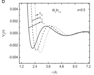
Figure 3 shows the profile of the effective partial pair potentials for an Al-based alloy namely AlxIn1-x. It is seen that partial pair potential has the sallowest potential well and the deepest well. That of lies in between. It is also seen that the position of the well minima for and shift to large relative to . Similar feature is also observed for transition metal segregation alloys ( for example Fex Cu1-x, Cux Co1-x). In case of ZnxBi1-x the amount of shift among different partial pair potentials is significantly small. This shifting is largely associated with the difference in the values of the core radii between individual components of the alloy. We note here that in random alloys generally lies between and . But in the case of compound forming alloys goes down the well of the or whichever has lower value. We note here that in the effective pair potential calculations Ichimaru-Utshumi dielectric function [59] has been used by Bhuiyan and his group because this function satisfies both compressibility
sum rule and the short range correlation function. The BS pseudopotential model has proven to be successful in the studies of liquid structure [60-63], thermodynamic properties [34,35,64,65], atomic transport [66-70] and electronic transport properties [71,72] of liquid metals and there alloys.
The partial pair correlation function, , is related to the partial interionic pair potential through the statistical mechanics[73] (see equation (7)). Partial pair correlation functions for three different concentrations are presented in figure 4. In the alloys, rich in component , exhibits the largest peak, while the trends become opposite in alloys rich in component ; that is shows the largest main peak. But in both cases peak value of remains in the middle of and . The physical significance of is that, it gives a measure of the probability of finding the number of nearest neighbours at a distance of the peak from the ion located at the origin. Thus the area under the principal oscillation provides the coordination number, a characteristic feature of the condensed matter. Advantage of it is that, can also be derived from the -ray or neutron diffraction data through the Fourier transformation, and directly from the computer simulation experiment. In the theoretical study of liquid metals it plays the central role in describing thermodynamic properties.
4.2 Energy of mixing
The free energy of mixing and its effects on the critical properties of segregation are described for different alloys below.
(a) LixNa1-x liquid binary alloys:
The first attempt to estimate the energy of mixing theoretically for Li1-xNax liquid binary alloys from a microscopic approach was made by Tamaki [74]. He also attempted to relate effective pairpotential between ions with the immiscibility of the segregating alloys (see Figure 5(a)). He was Stroud who made an attempt systematically for the first time to understand the segregating properties such as critical concentration and critical temperature of Li1-xNax liquid binary alloys using a microscopic theoretical approach [23]. He employed there the electronic theory of metal based on the empty core model [75], statistical mechanics and the Gibbs-Bogoliubov variational scheme [76] in order to calculate the free energy of mixing.
(a) (b)
(b)
Figure 5(b) shows a schematic diagram, presented by Stroud in [23], for the as a function of concentration for different temperatures. For the energy of mixing profile are concave upward for all concentrations, which manifests complete miscibility (i.e. alloy is stable against segregation) at any concentration. But for the profile becomes concave downward at some concentrations which indicates segregation of the alloy. The temperature at which spinodal points and coincides is called the critical temperature , and the concentration at which it happens is called the critical concentration . Here, in the calculation the Hubbard type dielectric function [77] is used. The critical concentration for LixNa1-x segregating alloy was found to be xc =0.7, but the predicted critical temperature was overestimated by one third
[23].
(b) AlxIn1-x liquid binary alloys:
This AlxIn1-x alloy is formed by the elemental metals Al and In. These elements belong to the less simple polyvalent metals. Al based alloys are known to be good candidates for a new advanced anti-friction materials. The input values such as potential parameters , and along with number density, , for Al and In, and also for some other elements are shown in Table 2.
| Elements | ||||
|---|---|---|---|---|
| Al | 0.0517 | 1.91 | 0.30 | 3.0 |
| In | 0.0342 | 1.32 | 0.29 | 3.0 |
| Bi | 0.0289 | 1.49 | 0.36 (0.35) | 3 (5) |
| Fe | 0.0756 | 1.425 | 0.33 | 1.5 |
| Co | 0.0787 | 1.325 | 0.27 | 1.5 |
| Cu | 0.0760 | 1.510 | 0.44 | 1.5 |
(a)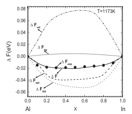 (b)
(b)
Faruk and Bhuiyan[21] studied the segregating properties of AlxIn1-x liquid binary alloys by using the electronic theory of metals (first principle calculations) along with the statistical mechanics and perturbative approach. Initially, they justified the appropriateness of the potential parameters by calculating static structure factors of the elemental liquids at a thermodynamic state at which experimental data are available [78]. Figure 6(a) shows the breakdown details of energy of mixing, , at 1173 K. It is noticed that the HS contribution to the energy of mixing is negative and values are the lowest among all other contributions across the whole range of concentrations. The tail part contribution is also negative across the concentration range and values are the second lowest among all others. Contribution of the electron gas, , is positive for the full concentration range and values
are very close to zero. The volume dependent (i.e. structure independent) part of the energy of mixing, , due to electron ion interaction is positive and large across the full range of concentration. The combined effect of all contributions, , agree well with the corresponding experimental data [79]. This signifies the accuracy of the approach for the study of energy of mixing at different temperatures.
The temperature dependent energy of mixing for AlxIn1-x liquid binary alloys for different concentrations are illustrated in figure 6(b). As temperature is decreased from 1173 K, increases gradually and at 1155 K becomes partially positive and partially negative. Further lowering of temperature increase the miscibility gap and at 1140 K the concentration gap span the whole range of concentration. A careful observation finds the first downward concavity or positivity of at 1160 K, and the concentration at which it happens is . So, the predicted critical temperature and concentration for AlxIn1-x segregating alloys are K and , respectively. The experimental work by Campbell et al.[80], and Campbell and Wagemann [9] report a critical temperature of 1220 K. whereas Predel [1] reports 1100 K for xIn1-x liquid binary alloys. Differential thermal analysis by Sommer et al. [81] reports 1112 K. The average of these scattered experimental data is 1144 K which is close to the theoretical prediction of Faruk and Bhuiyan[21]. The experimental critical concentration [10,1] is 0.5 which is exactly the same as that of theoretical prediction
[21]. But the experimental
data reported in [9] is 0.34 which largely deviates from 0.5.
(a) (b)
(c) BixAl1-x liquid binary alloys:
BixAl1-x liquid binary alloy is formed by two elements Al and Bi which belong to group IIIB and VB in the periodic table, respectively. The melting points of Al and Bi are 933 and 544 K, respectively; the corresponding densities are 2.375 and 9.78 gm cm-3. Al is a trivalent and Bi is a pentavalent metal. The atomic radii of Al and Bi are 1.82 and 1.63 Å, respectively. The large mismatch in their physical properties makes this alloy interesting to study theoretically.
Figure 7(a) illustrates the breakdown details of the energy of mixing at 1187 K at which some experimental data [79] for are available in the literature. The HS contribution to the energy of mixing is negative for the whole concentration range as is found for AlxIn1-x liquid binary alloys. But unlike AlxIn1-x, the tail part contribution, , of BixAl1-x alloys is positive for all concentrations with a maximum near equiatomic concentration. The volume dependent part, , in this case, is positive but the magnitudes are much lower than that of . The electron gas contribution, , is nearly zero as for AlxIn1-x. The combined effect of all contributions to the free energy, however, agrees well with the experimental results at
1173 K available in the literature [79].
Figure 7(b) shows the energy of mixing for BixAl1-x liquid binary alloys for different temperatures. It appears that the alloy exhibits a
complete miscibility at 1350 K, and immiscibility for all concentrations at 1050 K. But at 1290 K, shows a partial positivity with concavity downward near 0.15.
Further decrease of temperature gradually enhances the concentration gap. As the concavity downward (or positivity) of manifests onset of segregation, one can conclude that
the predicted critical concentration is , and critical temperature 1290 K, while the corresponding experimental values are [82] and [82,83].
(a) (b)
(d) ZnxBi1-x liquid binary alloys:
Figure 8(a) shows the free energy of mixing for liquid ZnxBi1-x alloys at 873 K [24]. is negative for ZnxBi1-x liquid binary alloys for the whole range of concentration, this trend is similar to that of the previous alloys, and having the smallest values relative to the other components for each concentration. In this case is asymmetric in nature where the minimum value is found to be around 0.6 which is located in the Bi rich alloys. and contributions are positive for the full range of concentrations, but shows the larger values than that of . contribution is nearly zero as other segregating alloys under consideration of
[21]this review article. The total energy of mixing, however, matches well with corresponding experimental data [79].
Temperature dependence of are illustrated in figure 8(b) It is noticed that at 773 K and higher temperatures is negative for all concentrations.
This nature indicates that the alloy is completely miscible in the regime of the above thermodynamic states. But at a lower temperature 673 K,
becomes positive i.e. concave downward for some concentrations and negative for others. When temperature is lowered further miscibility gap increases gradually as previous systems
and cover the whole concentration range at 550 K. From figure it appears that the critical concentration is and the critical temperature K.
The experimental value for is 0.83 [16,17], the critical concentration found theoretically by Stroud [36] and Karlhauber et al [84] (from quasi lattice theory)
was =0.75 and 0.87, respectively. Experimental critical temperatures are 856 K [16] and 878 K [17], and a theoretical study shows 438 K [36].
(a) (b)
(e) FexCu1-x liquid binary alloys:
Figure 9(a) shows that the HS contribution to the free energy of mixing for FexCu1-x is negative for all concentrations at K [22]. Here the tail part contribution to the energy of mixing is negative for all concentrations unlike other segregating alloys. The volume dependent term is
positive for the whole
concentration range, and the electron gas
contribution is almost zero as for all others discussed above. The total energy of mixing obtained summing all four contributions is negative
for all concentrations and the agreement with available measured data [79] is fairly good. At K the alloys remain miscible across the full concentration range.
As temperature is lowered to 100 K, becomes partially positive around equiatomic concentration where the concavity is downward, and the other part of energy
of mixing remains negative with upward concavity.
The critical temperature thus found was and the critical concentration found was 0.5. The experimental values reported by different authors for
are 0.56 [13], 0.538 [14] and 0.538 [15], and the corresponding experimental data for are 1696, 1704 K and 1694 K, respectively.
(f) CoxCu1-x liquid binary alloys:
In this case the behaviour of various contributions to is found to be similar to that of FexCu1-x [22]. But, in the immiscible state shows (Figure 10) an asymmetric feature with a value of critical concentration 0.58 and critical temperature 1650 K. The corresponding experimental values are 0.53 and 1547 K [12].
Bhuiyan and coworkers carefully investigated why varies with
temperature. They have found that and are sensitive to T and are mostly responsible for the variation. While and are not sensitive to T at all. The sensitivity arises, in this case, due to the alteration of and consequently , with the change of .
4.3 Enthalpy of mixing
(a) BixAl1-x liquid binary alloys:
The enthalpy of mixing, , are used as a probe to study the critical properties of BixAl1-x liquid binary alloys. Figure 11 demonstrates that calculated values of enthalpy of mixing agree in an excellent way with available experimental data for miscible alloys at 1187 K [79]. However, figure also show that the trends of as a function of concentration is just opposite like a mirror reflection to that of free energy of mixing discussed above. That is at 1350 K is positive, and at 1050 K it is negative for the full concentration range, while at the same thermodynamic states shows negative and positive values, respectively. Figure also shows that, at about 1290 K, exhibits negative (i.e. concave upward) at low values of and positive (i.e. concave downward) for the rest. That means segregation of the alloy begins at 1290 K which is exactly same as found from [25]. But in the
case of enthalpy of mixing the critical concentration is found to be somewhat smaller than predicted by the energy of mixing [25].
4.4 Enropy of mixing
It is interesting to see how another static magnitude the entropy of mixing describes the critical properties of segregation for different alloys.
(a) (b)
(a) ZnxBi1-x liquid binary alloys
Figure 12(a) shows the breakdown details of different contributions to the total entropy of mixing calculated by Kasem et al. [24]. It is seen from figure that at 873 K,
is negative
up to and then becomes positive. is negative in the concentration interval , and positive beyond it. Contribution
of HSD mismatch term, , is almost zero across the whole range of concentration. The tail part contribution, ,
is found to be positive for the full concentration range. However, the combined effect of these contributions that is the total entropy of mixing
is positive for all concentrations and, the agreement
between theory and experiment is very good up to , and fairly good for [79].
Figure 12(b) shows the temperature dependence of entropy of mixing for ZnxBi1-x liquid binary alloys [24]. We note here that negativity of
(i.e. upward concavity) is an indication of segregation.
Figure also shows that the critical temperature and critical concentration are 773 K and , respectively. These values are found to be same as
that found from the energy of mixing [24].
(b) BixAl1-x liquid binary alloys
Figure 13 shows entropy of mixing for BixAl1-x liquid binary alloys calculated by Fysol et al. [25]. At K, is positive for all concentrations and at K
it is negative for the whole range of concentration. For temperatures in between the entropy of mixing is partly positive and partly negative. Fysol et al. [25] theoretically
found the values 0.1 and K for critical concentration and critical temperature, respectively. Here the value of is the
same as that found from [25] but is somewhat lower in this case.
5 Concluding remarks
Looking at figures of free energy of mixing for AlxIn1-x, FexCu1-x, CuxCo1-x, ZnxBi1-x, and BixAl1-x liquid binary alloys one can easily find that the HS
contribution is always negative for all concentrations and temperatures. This means that, HS liquid alone cannot describe segregation for binary alloys. This finding agrees with that of Libowitz and Rowlinson [40]. However, becomes positive for the whole range of concentration and dominates other contributions in the case of FexCu1-x, CuxCo1-x, and AlxIn1-x liquid binary alloys; this feature directly favours the
| xc | Tc (K) | ||||
| Systems | (Theo.) | (Expt.) | (Theo.) | (Expt.) | Others(Theo.) |
| AlIn | 0.5 | 0.5, 0.34 | 1160 | 1155, 1150, 1145 | - |
| FeCu | 0.5 | 0.56, 0.538 | 1750 | 1696,1704,1694 | - |
| CuCo | 0.58 | 0.53 | 1650 | 15473 | - |
| ZnBi | 0.9 | 0.83 | 773 | 856, 878 | 438 |
| BiAl | 0.15 | 0.19 | 1290 | 1310 | - |
segregation for these alloys. The contribution of the tail part of the pair potential, , becomes positive for the full concentration range for ZnxBi1-x, and BixAl1-x liquid binary alloys and negative for others. The electron gas contribution is nearly zero for all systems and for any thermodynamic state characterized by temperature. Energy of mixing for hard sphere liquid and the tail part contribution are very sensitive to temperature unlike and . In the case of free energy and increases with increasing temperature, as a result total energy of mixing becomes concave downward which manifests immiscibility of the alloy. The values of the critical temperatures and critical concentrations for different alloys are illustrated in Table 3.
Understanding of the segregating behaviour of liquid binary alloys from the microscopic theory for transport properties has just began. Some interesting features exhibited by the coefficient of viscosity and diffusion coefficient as a function of concentration appears to be spectacular [25]. One of the features is the sharp bending in the vs (or vs ) profile around the
critical concentration. Competition between the thermal excitation of ions and the variation of density with temperature is another one. In this case, for , effects of atomic excitation dominates in determining the dynamics whereas this situation reverses for , that is the effect of density variation with temperatures dominates the excitation effects. The third interesting feature is the existence of a kind of scaling behaviour with , near the critical temperature. These novel features showed by some segregating liquid binary alloys demands further research to understand the dynamic effects in segregating alloys.
6 Appendix
The softness parameter used in the calculation are determined by fitting experimental at small (see Fig.12).

References
B. Predel, Z. Metall 56, 791 (1965).
H. J. Axon, Nature 162, 997 (1948).
A. R. Miedema, P F de Chatel and F R de Boer, Physica 100B, 1 (1980).
J M Cowley, Phys. Rev. 77, 667 (1950).
B E Warren, X-ray Diffraction (Reading, M. A: Addison-Wesley, 1969).
E A Guggenheim, Mixtures (Oxford, Oxford University Press, 1952).
I Pregogine, The molecular theory of solutions (New York: North-Holland, 1957).
A. B. Bhatia and R. N. Singh, Phys. Chem. Liq. 13, 177 (1984).
A N Campbell and R Wagemann, Can. J. Chem. 44, 657 (1966).
B Predel and H Sandig, Mat. Sci. Eng. 4, 49 (1969).
L. Ratke and S. Diefenbach, Mat. Sci and Eng. R15,263 (1995).
C D Cao, G P Gorler, D M Herlach and B Wei, Mater. Sci. Eng. A 325, 503 (2002).
D Nakagawa, Acta Metall. 6, 704 (1958).
G Wilde, R Willnecker, R N Singh and F Sommer, Z. Metall. 88, 804
(1997).
C P Wang, X J Liu, I Ohnuma, R Kainuma and K Ishida, J. Phys. Edu. Diffus. 25, 320 (2004).
D V Malakhov, CALPHAD 24, 1, 2000.
G D Wignall and P A Egelstaff, J. Phys. C: Solid State Phys. 1, 1088 (1968).
Z Fan, S Ji, and J Zhang, Mater. Sci. Tech. 17, 837, 2001.
W Hoyer, I Kaban and M Merkwitz, J. optoelec. Adv. Material 5,1069 (2003).
I G Kaban, and W Hoyer, Phys. Rev. B 77,12546 (2008).
Mir Mehedi Faruk, G.M. Bhuiyan, Physica B 422, 156 (2013).
Mir Mehedi Faruk, G.M. Bhuiyan, Amitabh Bishwas, and Md. Sazzad Hossain. J. Chem. Phys. 140, 134505 (2014).
D. Stroud, Phys. Rev. B, 7 4405 (1973).
Md. Riad kasem, G. M. Bhuiyan and Md. Helal Uddin Maruf, J. Chem. Phys. 143, 034503 (2015).
Fysol Ibna Abbas, G M Bhuiyan and Riad Kasem, J Phys. Soc. Japan 89, 114004 (2020).
R. N. Singh and F Sommer, Rep. Prog. Phys. 60, 57 (1997).
J Blanco, D J Gonzalez, L E Gonzalez, J M Lopez and M J Stott, Phys Rev. E 67, 041204 (2003).
H Rupersberg and W Knoll, Z Naturfor a 32, 1314 (1977).
N March, S Wilkins and J E Tibbals, Cryst. Latt. Defects 6, 253 (1976).
A B Bhatia and R N Singh, Phys. Chem. Liq. 11, 285 (1982).
N H March, Phys. Chem. Liq. 20, 241 (1989).
Y A Odusote, L A Hussain, O E Awe, J Non-Cryst. Solids 353, 1167 (2007).
M. Shimoji, Liquid Metals: An Introduction to the Physics and Chemistry of Metals in the liquid State ( Academic Press, London. 1977).
G M Bhuiyan and A Z Ziauddin Ahmed,, Physica B 390, 377 (2007).
G. M. Bhuiyan, Md. Saiful Alam, A. Z. Ziauddin Ahmed, Istiaque M. Syed and R. I. M. A. Rashid, J. Chem. Phys. 131 (2009).
D. Stroud, Phys. Rev. B, 8, 1308 (1973).
J.Hafner, From Hamiltonoians to Phase Diagrams (Springer, Berlin, 1987) p. 56.
I. H. Umar, A. Meyer, M. Watabe and W. H. Young, J. Phys. F. 4, 1691 (1974a).
J. L. Lebowitz, Phys. Rev. 133, A895 (1964).
J. L. Lebowitz and J.S. Rowlison, J. Chem. Phys. 41, 133 (1964).
S. A. Rice and A. R. Alnatt, J. Chem. Physics. 34, 2144 (1961).
A. R. Alnatt and S. A. Rice, J. Chem. Physics. 34, 2156 (1961).
M. Kitajima, T. Itami and M. Shimoji, Phil. Mag. 30,285 (1974).
N W Ashcroft and N D Mermin, Solid State Physics (Holt, Rinehart and Winston, 1976)
M P Marder, Condensed Matter Physics (John Wiley and Sons, Hoboken, Newjersey, 2010)
R M Zief, G E Uhlenbeck and M Kac, Phys. Report 32, 169 (1977).
M. W. Zymansky and R. H. Dittman, Heat and Thermodynamics (The Mcgraw-Hill Company Inc., New York, 1997) 7th ed..
R K Pathria, Statistical Mechanics (Pergamon Press, Oxford, 1985).
Mehran Kardar, Statistical Physics for Particles (Cambridge University Press, Chembridge, 2007).
N. W. Ashcroft and D. C. Lagrength, Phys. Rev. 156, 685 (1967).
J. D. Weeks, D. Chandler and H.C. Andersen, J. Chem. Phys. 55, 5422-5423 (1971).
A. Meyer, M. Silbert, and W. H. Young, Chem. Phys. 49,147 (1984).
H C Andersen, D Chandler and J D Weeks, Adv. Chem. Phys. 34, 105 (1976).
G D Mahan, Many-particle Physics, (Plenum Press, New York, 1983) p 459.
P Protopapas. H C Andersen and N A D Parlee, J. Chem. Physics 59, 15 (1973).
J. L. Bretonnet and M. Silbert, Phys. Chem. Liq. 24, 169 (1992).
A B Bhatia and D E Thornton, Phys. Rev. B 9, 435 (1970).
R N Singh and F Sommer, Z. Metall. 83, 7 (1992).
S. Ichimaru, K. Utsumi, Phys. Rev. B 24, 7385 (1981).
G. M. Bhuiyan, J. L. Bretonnet, L.E. González, M. Silbert, J. Phys. Condens. Matter 4, 7651 (1992).
G. M. Bhuiyan, J. L. Bretonnet and M. Silbert, J. Non-Cryst. Solids 145, 156 (1993).
M. A. Khaleque, G. M. Bhuiyan, S. Sharmin, R. I. M. A. Rashid, S. M. Mujibur Rahman, Eur.Phys.J. B 26, 319 (2002).
J. L. Bretonnet, G. M. Bhuiyan and M. Silbert, J. Phys. Condens. Matter 4, 5359 (1992).
Fysol Ibna Abbas, G. M. Bhuiyan and Md. Riad kasem, J. Non-Cryst. Solids 481, 391 (2018).
F. Zahid, G. M. Bhuiyan, S. Sultana, M.A. Khaleque, R.I.M.A. Rashid and S. M. Mujibur Rahman, Phys. Status Sol. B 215, 987 (1999).
G. M. Bhuiyan, I. Ali and S. M. Mujibur Rahman, Physics B 334,147 (2003).
E. H. Bhuiyan, A. Z. Ziauddin Ahmed, G. M. Bhuiyan M. Shahjahan, Physica B 403,1695 (2008).
S Chanda, A Z Ziauddin Ahmed, G M Bhuiyan, S K Barman and S Sarker, J. Non-Cryst. Solids 357, 3774 (2011).
A B Patel and H Sheng, Phys. Rev. B 102, 064101 (2020).
M A Mohaiminul Islam, R C Gosh and G M Bhuiyan, J. Mol. Liq. 290, 111224 (2019).
S. Sharmin, G. M. Bhuiyan, M. A. Khaleque, R.I.M.A. Rashid and S. M. Mujibur Rahman, Phys. Status Sol B 232,243 (2002).
M D Salah Uddin, R C Gosh and G M Bhuiyan, J Non-Cryst. Solids 499, 426 (2018).
D. A. McQuarrie, Statistical Mechanics (Harper and Row, New york, 1976).
S. Tamaki, Phys. Lett. A 40, 17 (1972).
N W Ashcroft, Phys. Lett. A 23, 48 (1966).
J A Moriarty, Phys. Rev. B 16, 2537 (1977).
J Hubbard, Proc. R. Soc. Lond. 243, 336 (1957).
Y. Waseda, The Structure of Non-Crystalline Materials (McGraw-hill, 1984).
R. Hultgren, P. D. Desai, D. T. Hawking, M. Gleiser and K. K. Keluey, Selected values of Thermodynamic Properties of Binary Alloys (American Society of Metals, 1973).
A N Campbell, L B Buchamann, J M Kuzmzk, R H Tuxworth, J. Am. Chem. Soc. 74, 1609 (1952).
B Predel, Z. Metallk, 56, 791 (1965).
F Sommer, H G Krull and S K Yu in: L Ratke (Ed), Immiscible Liquid Metals and Organics, DGM- Informationsgesellschaft, (1993) p.79.
A. J. McAllster, Bull. Alloy Phase Diag. 5, 247 (1984).
V. Raghavan, J. Phase Equil. Diffus. 33, 166 (2012).
S Karlhuber, A Mikula, R N Singh and F Sommer, J Alloys and Comp. 283, 198 (1999).