In the preceding work[13], we discussed that a randomly branched polymer is a mixture of a variety of isomers: a linear polymer, star polymers, irregularly branched polymers, and dendrimers. One way to classify such diverse isomers is to characterize the spacial configurations according to the asymptotic relation, $\left\langle s_{N}^{2}\right\rangle_{0}\propto N^{2\,\nu_{0}}$ for $N\rightarrow\infty$, between the radius of gyration and the total mass. As has been well-established, an unperturbed randomly-branched-polymer has the exponent, $\nu_{0}=\tfrac{1}{4}$, whereas the linear, star, and comb polymers have the exponent $\nu_{0}=\tfrac{1}{2}$, and the dendrimers have $\nu_{0}=0$. A randomly branched polymer has just the intermediate exponent between $1/2$ and 0. To date, within our knowledge, no single branched polymer having $0<\nu_{0}<1/2$ has been reported. In this study, we focus on a special comb polymer with side chains comparable in length to the backbone.

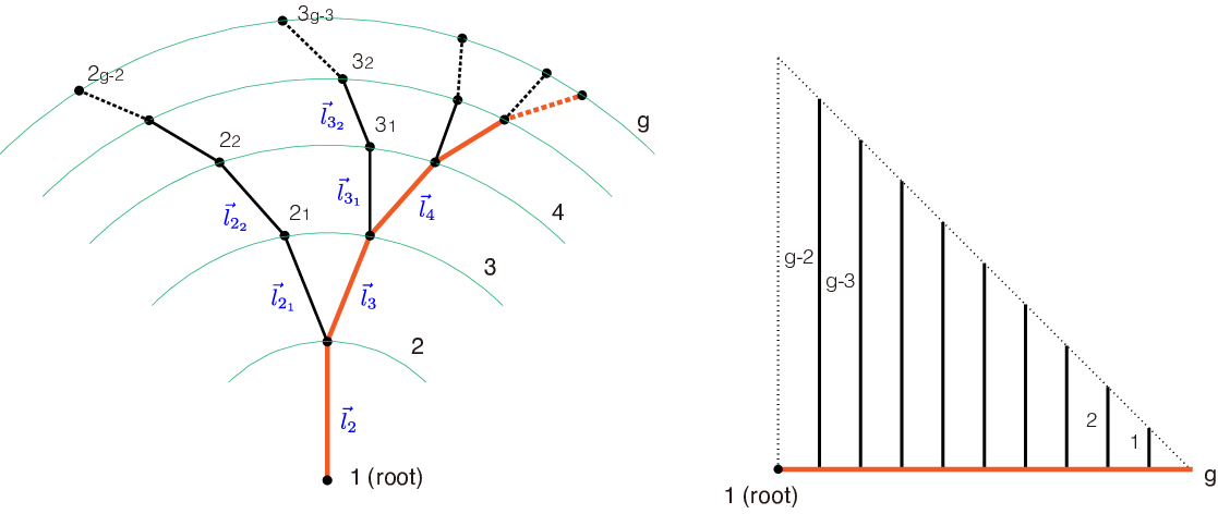
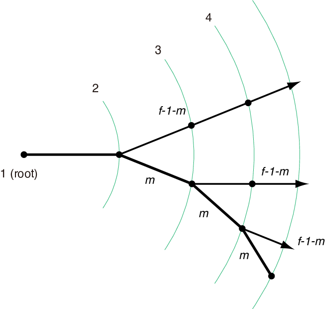
It has been shown experimentally[10] that comb polymers with various lengths of side chains, equally, behave as a linear polymer. It seems obvious that, given $N\rightarrow\infty$, those findings can be generalized to all comb polymers that have finite lengths of side chains. On the basis of those findings, we examine, in this paper, a special comb polymer having long side chains that grow indefinitely in parallel with the growing backbone. One of such polymers is illustrated in Fig. 1; this polymer has a geometry that can be deformed to the isosceles right triangle, so that all the end monomers on the side chains have the same generation number, $g$, as the main backbone (red bold-line). So, irrespective of the size of $g$, this comb polymer preserves the same geometric structure. For this reason, we name this special polymer triangular polymer. At first sight, such a polymer might appear to be an artificial construct. On the contrary, this is a real object that must be necessarily formed, in a certain probability, in the process of the random branching reactions under the principle of the equal reactivity of functional units (ERF)[5].

Let the triangular polymer be constructed from $g$ generations. Then, index the branching units on the backbone from 1 (root) to $g$, while for the units on the side chains from $k_{1}$ to $k_{g-k}$, where $k_{i}$ signifies the $i$th monomer on the side chain emanating from the $k$th generation ($i=1,\cdots,g-k$); for instance, $3_{2}$ denotes the second monomers on the side chain emanating from the branching unit on the third generation (Fig. 1). So we consider each side chain to be a part of the corresponding monomer on the main backbone. Let $u_{g_{i}}$ represent the total number of monomers belonging to the branching unit on the $i$th generation: for instance, $u_{g_{1}}=1$, $u_{g_{2}}=1+(g-2)$, $u_{g_{3}}=1+(g-3)$, and so forth. The sum of the number of monomer units from $i=1$ to $k$ is

The total number of branching units of this polymer is, therefore,

To calculate the mass distribution function, we make use of the Isihara Formula[3, 4]:

As we have discussed in the preceding paper[13], the end-to-end distance, $\vec{r}_{Gp}$, from the center of gravity to the $p$th monomer can be expressed by the sum of bond vectors having unequal step lengths: $\vec{r}_{Gp}=\sum_{j}c_{j}\,\vec{l}_{j}$[9, 12]. So, our task is only to decompose the end-to-end vector, with the help of the Isihara formula[3, 4], into the sum of every bond vector that constitutes the polymer. Let the monomer 1 be located on the root. It is convenient to redefine $c_{k}$ as the coefficient for $\vec{l}_{k+1}$, where $\vec{l}_{k+1}=\vec{r}_{G(k+1)}-\vec{r}_{Gk}$. For the vectors on the side chains, we add the small subscript, $i$, such that $(k+1)_{i}$. Clearly, the coefficient, $c_{k}$, represents the number of trails that pass through the bond in question. According to Fig. 1, it follows that

Then the result is

for $p=1$

$$\vec{r}_{G1}=-\frac{1}{N}\sum_{k=1}^{g-1}\Bigg[(N-u_{k})\,\vec{l}_{k+1}+\sum_{i=1}^{g-k-1}(g-k-i)\,\vec{l}_{(k+1)_{i}}\Bigg]$$

(6)

for $p=2$

$$\vec{r}_{G2}=\frac{1}{N}\left\{\left[N-(N-u_{1})\right]\,\vec{l}_{2}-\sum_{k=1}^{g-1}\Bigg[(N-u_{k})\,\vec{l}_{k+1}+\sum_{i=1}^{g-k-1}(g-k-i)\,\vec{l}_{(k+1)_{i}}\Bigg]+(N-u_{1})\,\vec{l}_{2}\right\}$$

(7)

$$\vec{r}_{G2_{j}}=\frac{1}{N}\Bigg\{\left[N-(N-u_{1})\right]\,\vec{l}_{2}+\sum_{i=1}^{j}[N-(g-1-i)]\,\vec{l}_{2_{i}}-\sum_{k=1}^{g-1}\Bigg[(N-u_{k})\,\vec{l}_{k+1}+\sum_{i=1}^{g-k-1}(g-k-i)\,\vec{l}_{(k+1)_{i}}\Bigg]\\ +[N-u_{1}]\,\vec{l}_{2}+\sum_{i=1}^{j}(g-1-i)\,\vec{l}_{2_{i}}\Bigg\}$$

(8)

where $1\leq j\leq g-2$.

for $p=3$

$$\vec{r}_{G3}=\frac{1}{N}\Bigg\{\sum_{k=1}^{2}\left[N-(N-u_{k})\right]\,\vec{l}_{k+1}-\sum_{k=1}^{g-1}\Bigg[(N-u_{k})\,\vec{l}_{k+1}+\sum_{i=1}^{g-k-1}(g-k-i)\,\vec{l}_{(k+1)_{i}}\Bigg]\\ +\sum_{k=1}^{2}[N-u_{k}]\,\vec{l}_{k+1}\Bigg\}$$

(9)

$$\vec{r}_{G3_{j}}=\frac{1}{N}\Bigg\{\sum_{k=1}^{2}\left[N-(N-u_{k})\right]\,\vec{l}_{k+1}+\sum_{i=1}^{j}[N-(g-2-i)]\,\vec{l}_{3_{i}}-\sum_{k=1}^{g-1}\Bigg[(N-u_{k})\,\vec{l}_{k+1}+\sum_{i=1}^{g-k-1}(g-k-i)\,\vec{l}_{(k+1)_{i}}\Bigg]\\ +\sum_{k=1}^{2}[N-u_{k}]\,\vec{l}_{k+1}+\sum_{i=1}^{j}(g-2-i)\,\vec{l}_{3_{i}}\Bigg\}$$

(10)

where $1\leq j\leq g-3$.

For the freely jointed chain, $\left\langle\vec{l}_{i}\cdot\vec{l}_{j}\right\rangle=0$ if $i\neq j$. The mean squares of the radius of gyration for respective vectors are therefore written in the form:

where $1\leq h\leq g$ for $\left\langle r_{Gh}^{2}\right\rangle$, and $2\leq h\leq g$ and $1\leq j\leq g-h$ for $\left\langle r_{Gh_{j}}^{2}\right\rangle$.

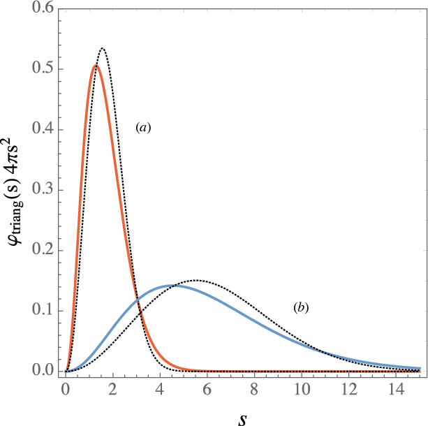
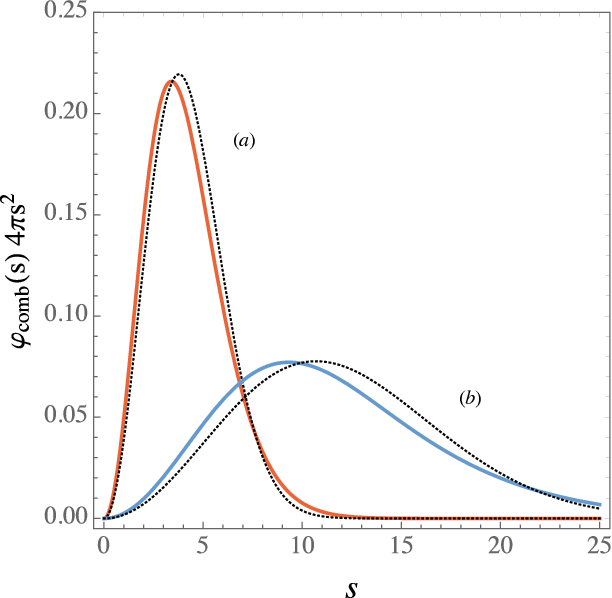
In Fig. 2, we plot the numerical solution of Eq. (15), with the help of Eqs. (13)-(14), for (a) $g=10$ ($N=46$) and (b) $g=100$ ($N=4951$). The dotted lines represent the Gaussian distribution functions having the same mean radii of gyration. There is a real difference between the exact distributions (solid lines: $-\hskip-1.70717pt-$ & $-\hskip-1.70717pt-$) and the Gaussian functions ($\cdots$).

In Table 1, we summarize the exponents for the ideal conformations of various polymers. To date, only three values of $\nu_{0}$ have been discovered, 1/2, 1/4, and 0, for polymeric compounds. No other exponent has been reported to date. The most prominent feature on the configurational statistics of polymers might be that the mean square of the radius of gyration can be written empirically in the form: $\left\langle s_{N}^{2}\right\rangle_{0}=A\,g\,l^{2}$ ($g\rightarrow\infty$), where $A$ is a polymer-species-dependent coefficient and also depends on the choice of the root monomer. To confirm this relationship, we have recast, in Table 2, the radii of gyration for various polymers in terms of $g$. It is seen that for all the polymers cited here, the mean squares of the radii of gyration take the form: $\left\langle s_{N}^{2}\right\rangle_{0}\propto g\,l^{2}$.

If we accept the empirical formula, $\left\langle s_{N}^{2}\right\rangle_{0}=A\,g\,l^{2}$, as a general rule, the problem of seeking the exponent, $\nu_{0}$, reduces to the problem of seeking the relationship between $g$ and $N$.

In the comb and the triangular polymers, we have, by definition, one backbone. We wish to extend this architecture to a more general case and apply the empirical rule, $\left\langle s_{N}^{2}\right\rangle_{0}=A\,g\,l^{2}$, to deduce the exponent without entering the intricate vectorial calculation. We have shown, in Appendix A, such an architecture, the extended triangular model, in which $m$ functional units (FU’s) branch off, whereas $f-1-m$ FU’s extend linearly. The resultant equation reads:

In this extended architecture, the triangular polymer in the text corresponds to the $m=1$ case with $f=3$ to yield $g\doteq\sqrt{N}$ and $\nu_{0}=1/4$, and the dendrimer the $m=f-1$ case to yield $g\doteq constant\cdot\log N$ and $\nu_{0}=0$. For $2\leq m\leq f-1$, the total mass has the form: $g\propto\log N$, which necessarily gives $\nu_{0}=0$. According to the above-mentioned empirical rule, there is no other exponent than 0 and 1/4 within this extended model.

Another possible architecture may be devised. An intriguing case is in the regular comb polymer theorized in Appendix B: This polymer has the total mass, $N=g+(g-1)n$. In the derivation in Appendix B, we have introduced $g$ and $n$ as constants and not variables. Let us alter the length of $n$, with $g$ being fixed. Then move $g$ to infinity. Given the finite length, $n$, of the side chains, we have $N\propto g$, and the exponent should take the value, $\nu_{0}=1/2$, whereas for a large $n$ comparable to $g$, we have $N\approx g^{2}$, and the exponent takes the different value, $\nu_{0}=1/4$, the value observed for the triangular polymer (Table 2). Along this line, it might be useful to introduce the general discrete function, $n=g^{t}$ ($t\geq 0$), with $g^{t}$ representing a set of integers. What we must be careful in introducing such a general function is that it might change the mathematical form of the empirical equation. To check this possibility, let us return to the original equation of the mean square of the radius of gyration for the comb polymer (Appendix B):

along with the relation: $N=g+(g-1)n$. Substituting $n=g^{t}$ into Eq. (B.13), we have, for $g\rightarrow\infty$,

together with $N\doteq g^{t+1}$. For $t>1$, we have $n>g$, and therefore it will be more proper to regard $n$ rather than $g$ as the main backbone. Then, making a variable transformation, $g^{t}\Rightarrow g^{\prime}$, we have $\left\langle s_{N}^{2}\right\rangle_{0}\propto g^{\prime}\,l^{2}$ $(t>1)$, showing that the above-mentioned empirical rule is still valid. On this basis, it will be useful to redefine the empirical equation in the form:

Substituting $g=N^{\frac{1}{t+1}}$ into Eq. (20), we have

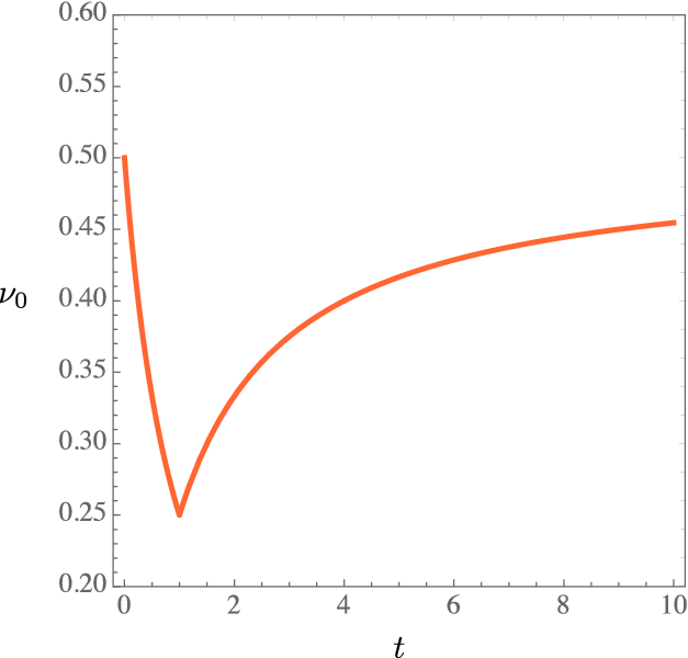
Eq. (22) has been plotted in Fig. 3 as a function of $t$. $t=0$ corresponds to the comb polymers with the finite length of $n$ and yields $\nu_{0}=1/2$, while $t=\infty$ corresponds to the case of the star polymers and again yields the value, $\nu_{0}=1/2$[2, 10, 13]. As one can see from Fig. 3, between these two extremes of $t$, $\nu_{0}$ can take any values within the interval, $1/4\leq\nu_{0}\leq 1/2$, for a sufficiently large $g$.

Then let us turn our attention to the lower region, $0\leq\nu_{0}\leq 1/4$. Our interest is whether or not there exist architectures that allow a large number of the exponents as well in this interval. To inspect this, we introduce a nested structure. The starting polymer ($N_{1}$) may have an arbitrary architecture. In Fig. 4, we have shown an example of $N_{1}$ being a linear polymer. The nesting rule is that on each nesting, a linear polymer with $g$ monomers is newly introduced as a backbone, on which the preceding structure is linked with each monomer on the new backbone. Such nesting is repeated successively to create deeper structures. Let $z$ represent the depth of the nest. Then, we can write generally $N_{z}=g+(g-1)N_{z-1}$. The solution to this recurrence relation is:

where $N_{1}$ can be any structures as mentioned above; for instance, $N_{1}=1$, $N_{1}=g$, $N_{1}(comb)=g+(g-1)n$, $N_{1}(triang)=g+\frac{1}{2}(g-1)(g-2)$, or so forth (Table 2).

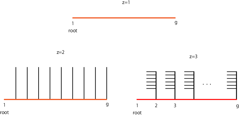
Here we consider the case that $N_{1}$ is a linear polymer. Substituting $N_{1}=g$ into Eq. (23) and taking the limit, $g\rightarrow\infty$, we have $N_{z}\propto g^{z}$. Then applying the empirical rule (21), we have $\left\langle s_{N}^{2}\right\rangle_{0}\propto(zgl)l$, so that for a fixed $z$, the mean square of the radius of gyration varies as $\left\langle s_{N}^{2}\right\rangle_{0}\propto zN^{\frac{1}{z}}l^{2}$, as $g\rightarrow\infty$. Hence

By substituting $z=1$, we recover $\nu_{0}=1/2$, the familiar value for the linear polymer; substituting $z=2$, we recover $\nu_{0}=1/4$, the value for the special comb polymers having $n=g$; for a large $z$ limit, Eq. (24) approaches the exponent, $\nu_{0}=0$, corresponding to the dendrimer as an ultimate structure. It is seen that, given the empirical rule (21), we can expect an infinite number of the exponents ($\nu_{0}=\frac{1}{2},\,\frac{1}{4},\,\frac{1}{6},\,\cdots$) in the interval, $0\leq\nu_{0}\leq 1/2$, corresponding to respective architectures from the linear polymer to the dendrimer.

The question may be raised about whether the architectures mentioned above (the comb polymers having side chains of the length, $g^{t}$, and the nesting structures) have a reality. Whether a polymer has a reality depends on the availability of the polymer through synthetic chemistry. In the sense that the above architectures can not be obtained, with a practical yield, by using the conventional random reaction, they will not be realistic. Nevertheless, not all these polymers are imaginal ones: from the thermodynamic point of view, the architectures having $\nu_{0}\geq 1/3$ can exist as it is, and some portion of the polymers having $\nu_{0}<1/3$ can exist in the expanded state, and hence, a considerable portion of the above polymers, in principle, can be constructed by step-by-step synthesis, given sufficient time and technology.

A noteworthy feature might be that, according to the theory of the excluded volume effects[7, 8, 13, 11, 16, 17] [for instance, $\nu=\frac{2(1+\nu_{0})}{d+2}$ ($d=3$) ^{† †\dagger2 † †\dagger2} $\dagger$2  We confine our discussion to $d=3$ since this formula has not been fully verified experimentally for the dimensions other than 3.], the present results imply the existence of a large number of the real exponents, $\nu$, corresponding to the respective ideal exponents, $\nu_{0}$.

The probability distribution of segments for the triangular polymer with a large $g$ can be expressed as the sum of the Gaussian functions having the mean squares of the end-to-end distances, $\left\{\left\langle r_{Gh}^{2}\right\rangle,\left\langle r_{Gh_{j}}^{2}\right\rangle\right\}$. It is found from Fig. 2 that there is a substantial deviation of the resulting formula (15) from the Gaussian function having the same mean square of the radius of gyration. On the other hand, in common with all the known polymers, the triangular polymer obeys the relationship:

where $g\,l$ is the contour length of the main backbone from the root to the youngest (outermost) generation, $g$.

As a reference polymer, we have calculated the probability distribution function (PDF) of segments for the regular comb polymer (Appendix B). As expected, the PDF of this polymer was found to be closer to the Gaussian function than that of the triangular polymer.

By virtue of the relationship (21^′), we might have gained a means to deduce the exponent, $\nu_{0}$, making use of the relationship between $N$ and $g$, without entering the intricate vectorial calculations. As an example, we have put forth, in Section 4, an extended comb polymer that has the side chains of the length, $n=g^{t}$, along with the total mass, $N\doteq g^{t+1}$ ($g\rightarrow\infty$). This leads us to the consequence: $\nu_{0}$ can take an arbitrary value in the interval, $1/4\leq\nu_{0}\leq 1/2$, by changing $t$ properly if $g$ is sufficiently large. We have put forth another example of the nested structures that create a continuous change of architectures from the linear chain molecule to the dendrimer. It is shown that, according to the empirical relationship (21^′), those new architectures give rise to a large number of the ideal exponents, $\nu_{0}=\frac{1}{2},\,\frac{1}{4},\,\frac{1}{6},\,\cdots$, in the interval, $0\leq\nu_{0}\leq 1/2$.

References

- [1] H. A. Kramers. The Behavior of Macromolecules in Inhomogeneous Flow. J. Chem. Phys. 14, 415 (1946).
- [2] B. H. Zimm and W. H. Stockmayer. The Dimensions of Chain Molecules Containing Branches and Rings. J. Chem. Phys., 17, 1301 (1949).
- [3] A. Isihara. Probable Distribution of Segments of a Polymer Around the Center of Gravity. J. Phys. Soc. Japan, 5, 201 (1950).
- [4] P. Debye, and F. Bueche. Distribution of Segments in a Coiling Polymer Molecule. J. Chem. Phys., 20, 1337 (1952).
- [5] P. J. Flory. Principles of Polymer Chemistry. Cornell University Press, Ithaca and London (1953).
- [6] G. R. Dobson and M. Gordon. Configurational Statistics of Highly Branched Polymer Systems. J. Chem. Phys., 41, 2389 (1964).
- [7] J. Issacson and T. C. Lubensky. Flory Exponents for Generalized Polymer Problems. J. Physique Letters, 41, L-469 (1980).
- [8]
(a) D. J. Klein. Rigorous results for branched polymer models with excluded volume. J. Chem. Phys. 75, 5186 (1981).
(b) W. A. Seitz and D. J. Klein. Excluded volume effects for branched polymers: Monte Carlo results. J. Chem. Phys. 75, 5190 (1981).
(c) D. J. Klein, W. A. Seitz, and J. E. Kilpatrick. Branched polymer models. J. Appl. Phys. 53(10), October, 6599 (1982). - [9] George H. Weiss and James E. Kiefer. The Pearson random walk with unequal step sizes. J. Phys. A: Math. Gen., 16, 489 (1983).
- [10]
(a) T. Yoshizaki, I. Nitta, and H. Yamakawa. Transport coefficients of helical wormlike chains. 4. Intrinsic viscosity of the touched-bead model. Macromolecules, 21, 165 (1988).
(b) Ken Terao, Yo Nakamura, and Takashi Norisuye. Solution Properties of Polymacromonomers Consisting of Polystyrene. 2. Chain Dimensions and Stiffness in Cyclohexane and Toluene. Macromolecules, 32, 711-716 (1999).
(c) Yo Nakamura. Dilute Solution Properties of Star and Comb Polymers. Kobunshi Ronbunshu, Vol. 57, No. 8, pp. 530-541 (2000).
(d) Yo Nakamura. Molecular Shape of Polymacromonomers in Solutions. SEN’I GAKKAISHI, 62, 48 (2006). - [11] Ch. von Ferber and Yu. Holovatch. Field-theoretical renormalization group analysis for the scaling exponents of star polymers. Condensed Matter Physics, 5, No1 (29), 117 (2002).
- [12]
(a) P. L. Krapivsky, and S. Redner. Random walk with shrinking steps. arXiv:physics/0304036 [physics.ed-ph]; Am. J. Phys. 72, 591-598 (2004).
(b) C. A. Serino and and S. Redner. Pearson Walk with Shrinking Steps in Two Dimensions. arXiv:0910.0852v3 [physics.data-an]; J. Stat. Mech. P01006 (2010). - [13]
(a) K. Suematsu. Radius of Gyration of Randomly Branched Molecules. arXiv:1402.6408 [cond-mat.soft] 26 Feb 2014.
(b) K. Suematsu. Excluded Volume Effects of Branched Molecules. arXiv:1606.03929v3 [cond-mat.soft] 29 Dec 2016.
(c) K. Suematsu. Volume Expansion of Branched Polymers. arXiv:1709.08883 [cond-mat.soft] 26 Sep 2017.
(d) K. Suematsu, Haruo Ogura, Seiichi Inayama, and Toshihiko Okamoto. Alternative Approach to the Excluded Volume Problem: The Critical Behavior of the Exponent . arXiv:1811.07280 [cond-mat.soft] 18 Nov 2018.
(e) K. Suematsu, Haruo Ogura, Seiichi Inayama, and Toshihiko Okamoto. Diffusion and Chemical Potential in Polymer Solutions. arXiv:1903.03950 [cond-mat.soft] 10 Mar 2019.
(f) K. Suematsu, Haruo Ogura, Seiichi Inayama, and Toshihiko Okamoto. Segment Distribution around the Center of Gravity of Branched Polymers. arXiv:2006.10130 [cond-mat.soft] 12 Jun 2020. - [14]
(a) P. Polinska, C. Gillig, J. P. Wittmer, and J. Baschnagel. Hyperbranched polymer stars with Gaussian chain statistics revisited. arXiv:1508.03733 [cond-mat.soft] 15 August 2015; Eur. Phys. J. E, 37: 12 (2014).
(b) M. Dolgushev, J. P. Wittmer, A. Johner, O. Benzerara, H. Meyerb and J. Baschnagel. Marginally compact hyperbranched polymer trees. Soft Matter, 13, 2499 (2017). - [15] Yingzi Yang, Feng Qiu, Hongdong Zhang, and Yuliang Yang. The Rouse Dynamic Properties of Dendritic Chains: A Graph Theoretical Method. Macromolecules, 50, 4007-4021 (2017).
- [16] V. Blabatska, K. Haydukivska, and Yu. Holovatch. Shape analysis of random polymer networks, arXiv:2001.07462v1 [cond-mat.dis-nn] 21 Jan 2020.
- [17] Khristine Haydukivska, Ostap Kalyuzhnyi, Viktoria Blavatska, Jaroslav Ilnytskyi. On the swelling properties of pom-pom polymers in dilute solutions. Part 1: symmetric case. arXiv:2012.00469v1 [cond-mat.soft] 1 Dec 2020.