Device-independent certification of Hilbert space dimension using a family of Bell expressions

Dimensionality is a fundamental property of a quantum system. The Hilbert space in which the quantum state belongs is an abstract construction but the number of dimension available to a system is a physical quantity and is considered to be resource for quantum computation and quantum information theory robin. Higher dimensional system can make a given protocol more efficient and alternatively, the security of many cryptographic protocols relies on the dimensional characteristics of the system. For example, instead of qubit system if four-dimensional states are used, then the celebrated Bennett-Brassard (BB84) cryptographic protocol bb84 can be shown to be entirely compromised acin06; brunner11. From the fundamental perspective, there are quantum correlations whose simulation by classical resources inevitably require dimensional superiority. The quantum dimension witness is a criterion that provides a lower bound on the dimension that is needed to reproduce a given measurement statistics. Of late, the device-independent dimension witness has become an important research area where the dimension of a quantum system is certified without requiring a priori knowledge about the devices used in the experiment.

The notion of dimension witness was first introduced in a seminal paper by Brunner et al.,brunner in the context of bipartite Bell scenario, which involve two spatially separated observers Alice and Bob, who access uncharacterized devices (black boxs). Alice and Bob receive inputs $x\in\{1,2,...n_{A}\}$ and $y\in\{1,2.....n_{B}\}$ respectively and the uncharacterized measurement device yielding respective outputs $a\in\{0,1\}$ and $b\in\{0,1\}$. The conditional probability $P(ab|xy)$ admits a $d$-dimensional representation if it can be written as; $P(ab|xy)=tr[\rho_{AB}(M_{a}^{x}\otimes M_{b}^{y})]$ for the state $\rho_{AB}$ $\in$ $\mathbb{C}^{d}\otimes\mathbb{C}^{d}$ shared between two parties and the local measurements $M_{a}^{x}$ and $M_{b}^{y}$ acting on $\mathbb{C}^{d}$. The reproduction of every joint probability $P(ab|xy)$ in quantum theory puts a lower bound on the dimension of the Hilbert space.

Since then flurry of interesting works along this direction have been reported wehner; gallego; dal12; brunnerprl13; guh14; bowler; bowlers; muk15; sik16; sik16prl; cai16; cong17; vin17; son17; cze18; str19; vin19; zha19; spee20. The work of Brunner et al., brunner was further generalized and extended to prepare measure scenario by Gallego et al., gallego and proposed a family of inequalities which serve as classical and quantum dimension witnesses are given by

where, $\alpha_{xy}=1$ if $x+y\leq N$ , and $\alpha_{xy}=-1$ otherwise. Here, $x\in\{1,2,....N\}$, $y\in\{1,2.....N-1\}$ and $E_{xy}$ is the correlation. The problem of dimension witness is meaningful if the number of preparation $(N)$ is greater than the Hilbert space dimension of the system. For classical states of dimension $d\leq N$ it is found that algebraic bound $I_{N}\leq L_{d}$, where $L_{d}=\dfrac{N(N-3)}{2}+2d-1$. For example $N=3$ and $d=2$ one finds the classical value is 3 and quantum value is $2\sqrt{2}+1$. Further analysis found that $I_{3}$ inequity is achieve its optimal value for $d=3$ which is $5$. So this inequality has the ability to test the dimension as well as to distinguish between the classical and quantum system.

Later, by assuming independence of the prepare and measure devices a non-linear dimension witness is also proposed bowler and test of dimension in communication network is also proposed bowlers. A connection to random access code wehner and to state discrimination brunnerprl13 are also pointed out. In a recent proposal, by employing binary-outcome measurements a certification of an arbitrary-dimensional quantum systems is proposed cze18. Experimental verifications of dimension witness including higher dimensional system has also been performed ahrens; hend; ahrens2; Ambrosio; zhu16; sun16; agulier; guo20.

In this paper we provide a family of quantum dimension witnesses based on the parity-oblivious random access code spek09. The parity oblivious condition imposed on Alice’s encoding scheme implies here that no parity information of the inputs of Alice is shared to Bob. It can be shown ghorai18 that the success probability of a $n$-bit random access code can be solely determined by a family of Bell expressions $(\mathcal{B}_{n})$ where Alice and Bob use $2^{n-1}$ and $n$ number of dichotomic measurements respectively. Importantly, for a given $n$, the optimal quantum value of $\mathcal{B}_{n}$ can only be achieved for the quantum system having local Hilbert space dimension $d=2^{\lfloor n/2\rfloor}$. The parity oblivious constraint is shown spekk05 to be equivalent to preparation non-contextuality assumption in an ontological model, and for a given $n$, such a constraint on the encoding scheme reduce the local bound of the family of Bell expressions $\mathcal{B}_{n}$ to preparation non-contextual bound spekk05. This is due to the fact that such a condition puts further restriction on free choices of the values of Alice’s observables.

For $n=2$ and $n=3$, the Bell expressions are well-known CHSH chsh and elegant Bell expressions gisin respectively. Since both the Bell expressions for $n=2,3$ can be optimized for qubit system, they cannot be served as dimension witness of Hilbert space. However, each of the Bell expressions for $n\geq 4$ has the potential to distinguish the dimensions $d=2^{m}$ of the Hilbert space with $m=1,2..2^{\lfloor n/2\rfloor}$ thereby serve as dimension witness of the Hilbert space. We provide explicit examples for $n=4,5$ and $6$ cases to demonstrate that the Bell expressions for both $n=4$ and $n=5$ certify qubit and two-qubit systems and for $n=6$ the relevant Bell expression certifies the qubit, two-qubit and three-qubit local systems.

Further, we examine the sharing of preparation contextuality by multiple sequential Bobs perform unsharp measurements. Using the family of Bell expressions mentioned above, it was shown asmita19 that the sharing of preparation contextuality can be demonstrated for arbitrary number of Bobs by using optimal quantum value of the family of Bell expressions, achieved for the $d=2^{\lfloor n/2\rfloor}$ dimensional Hilbert space. We argue that that there is a possibility of sharing preparation contextuality by arbitrary number of Bobs for the system in lower dimensional Hilbert space. We provide explicit example for $n=5$ where the number of sequential Bobs sharing preparation contextuality remains same for qubit and two-qubit system. Similarly, for $n=6$ the sharing is for possible for same number of sequential Bobs for qubit, two-qubit and three qubit systems. However, the value of unshrapness parameter required for demonstrating preparation contextuality by sequential Bob is always higher in lower dimensional system, as expected.

This paper is organized as follows. In Sec. II, we briefly recapitulate the essence of parity-oblivious random-access-code and derivation of the family of preparation non-contextual inequalities, i.e., the Bell inequalities those serve as the dimension witnesses. In Sec.III, we provide the sum-of-square approach to optimize the dimension witnesses for various dimensional quantum systems. We provide the specific examples for $n=4,5$ and $6$ to demonstrate how the corresponding Bell inequalities certify the $2^{m}$ dimensional systems in Sec. IV. For the dimension witnesses for $n=4,5$ and $6$, we examine the sharing of preparation contextuality by multiple Bobs for qubit, two-qubit and three-qubit systems in Sec. V. Finally, we summarize our work in Sec. VI.

Since the family of dimension witnesses is based on the parity-oblivious random access code (PORAC) and the parity-oblivious condition is equivalent to preparation non-contextuality assumption in an ontological model of an operational theory, we first provide the essence of preparation non-contextuality and then, the derivation of local and preparation non-contextual bound of the aforementioned family of Bell expressions.

We start by encapsulating the notion of an ontological model reproducing the quantum statistics hari; spekk05. In quantum theory, a preparation procedure $(P)$ produces a density matrix $\rho$ and the measurement procedure $(M)$ which is in general described by a suitable positive-operator-valued-measure (POVM) $E_{k}$, provides the probability of occurrence an outcome $k$ is given by $p(k|P,M)=Tr[\rho E_{k}]$, which is the Born rule. In an ontological model of quantum theory, the preparation of quantum state $\rho$ by a specific preparation procedure $P$ is equivalent to preparing a probability distribution $\mu_{P}(\lambda|\rho)$ in the ontic state space, satisfying $\int_{\Lambda}\mu_{P}(\lambda|\rho)d\lambda=1$ where $\lambda\in\Lambda$ and $\Lambda$ is the ontic state space. The probability of obtaining an outcome $k$ is a response function $\xi_{M}(k|\lambda,E_{k})$ satisfying $\sum_{k}\xi_{M}(k|\lambda,E_{k})=1$ where a measurement operator $E_{k}$ is realized through a measurement procedure $M$. The primary requirement of such an ontological model is to reproduce the Born rule, i.e., $\forall\rho$, $\forall E_{k}$ and $\forall k$, $\int_{\Lambda}\mu_{P}(\lambda|\rho)\xi_{M}(k|\lambda,E_{k})d\lambda=Tr[\rho E_{k}]$.

The notion of non-contextuality was reformulated and generalized for any operational theory by Spekkensspekk05. For our purpose, we focus on the quantum theory here. An ontological model of quantum theory can be considered to be preparation non-contextual if $\forall M:p(k|P,M)=p(k|P^{\prime},M)\Rightarrow\mu_{P}(\lambda|\rho)=\mu_{P^{\prime}}(\lambda|\rho)$ is satisfied where $P$ and $P^{\prime}$ are two distinct preparation procedures but in the same equivalent class kunjwal; mazurek; hameedi; pan19.

As mentioned, the family of dimension witnesses in the present work are derived through a two-party communication game known PORAC. It was shown by Spekkens spek09 that the parity-oblivious condition in an operational theory can equivalently be cast into the assumption of preparation non-contextuality in an ontological model. It is already shown in ghorai18 that the success probability of a $n$-bit PORAC can be solely linked with a family of Bell’s inequities. For the sake of completeness, we briefly encapsulate encapsulate the essence of the derivation.

In a $n$-bit PORAC, Alice chooses her bit $x^{\delta}$ randomly from $\{0,1\}^{n}$ with $\delta\in\{1,2...2^{n}\}$. The relevant ordered set $\mathcal{D}_{n}$ can be written as $\mathcal{D}_{n}=(x^{\delta}|x^{i}\oplus x^{j}=111...11\;\text{and}\;i+j=2^{n}+1)$ and $i\in\{1,2,...2^{n-1}\}$. Here, $x^{1}=00...00,x^{2}=00...01,....$, and so on. Bob can choose any bit $y\in\{1,2,...,n\}$ and recover the bit $x^{\delta}_{y}$ with a probability. The condition of the task is the following; Bob’s output must be the bit $b=x^{\delta}_{y}$. The parity-oblivious constraint here is that no information about any parity of $x$ can be transmitted to Bob. Following spek09, we define a parity set $\mathbb{P}_{n}=\{x|x\in\{0,1\}^{n},\sum_{r}x_{r}\geq 2\}$ with $r\in\{1,2,...,n\}$. For any arbitrary $s\in\mathbb{P}_{n}$, no information about $s.x=\oplus_{r}s_{r}x_{r}$ (s-parity) is to be transmitted to Bob, where $\oplus$ is sum modulo $2$.

In an operational theory, Alice encodes her $n$-bit string of $x^{\delta}$ prepared by a procedure $P_{x^{\delta}}$. Next, after receiving the particle, for every $y\in\{1,2,...,n\}$, Bob performs a two-outcome measurement $M_{n,y}$ and reports outcome $b$ as his output. Then the probability of success is given by

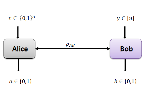
In quantum PORAC, Alice encodes her $n$-bit string of $x^{\delta}$ into quantum states $\rho_{x^{\delta}}$, prepared by a procedure $P_{x^{\delta}}$. On a suitable entangled state $\rho_{AB}$ = $|{\psi_{AB}}\rangle\langle{\psi_{AB}}|$ with $|\psi_{AB}\rangle\in\mathbb{C}^{d}\otimes\mathbb{C}^{d}$, Alice performs one of the $2^{n-1}$ projective measurements $\{{P_{A_{n,i}}}$, $\mathbb{I}-P_{A_{n,i}}\}$ where $i\in\{1,2,...2^{n-1}\}$ to encode her $n$-bits into $2^{n}$ quantum states are given by-

with $i+j=2^{n}+1$.

In quantum theory, the parity-oblivious condition implies that

In ontological model of quantum theory, the parity-obliviousness in Eq.(4) condition is equivalent to the preparation non-contextual assumption, i.e.,

Note that the number of parity-oblivious conditions for $n$-bit PORAC is the number of element in $\mathbb{P}_{n}$ ghorai18. We noticed that there are two types of parity oblivious conditions. The one arising from the natural construction, such as, $\mathbb{I}=P_{A_{n,i}}^{+}+P_{A_{n,i}}^{-}$. In that case, $s\in\mathbb{P}_{n}$ follow the property $\sum_{y}s_{y}=2m$ with $m\in\mathbb{N}$. For the rest of $s\in\mathbb{P}_{n}$ not satisfying the above property, a non-trivial constraints on Alice’s observables need to be satisfied are given by

The total number of such non-trivial constraints on Alice’s observables is $C_{n}=2^{n-1}-n$.

The measurements of for decoding scheme are taken to be

The quantum success probability can then be written as

where $\mathcal{B}_{n}$ is the family of Bell expressions is given by

which serve as the family of dimension witnesses in the present work. Note that, the Bell expressions in Eq.(10) provides the CHSH and Gisin’s elegant Bell’s inequality for $n=2$ and $n=3$ respectively and the corresponding local bounds are 2 and 6. The local bound of the family of Bell expressions for any arbitrary $n$ is given by ghorai18

However, the parity-oblivious condition in the usual RAC imposes a functional relationship between Alice’s observables as given by Eq. (6). This means that Alice choices of values are restricted and the local bound of Eq. (10) gets reduced (which we call preparation-noncontextual bound spek09; ghorai18) to

Since for any $n$, we have $(\mathcal{B}_{n})_{pnc}\leq(\mathcal{B}_{n})_{local}$ then for a given $n$, even if optimal quantum value $(\mathcal{B}_{n})_{Q}$ does not violate the local bound in Eq. (11), it may still reveal non-classicality by violating the preparation non-contextual given by Eq. (12). Note that, it is already known ghorai18 that the optimal quantum value of $\mathcal{B}_{n}$ can be obtained for the local system having dimension $d=2^{\lfloor n/2\rfloor}$. Our purpose here to examine the maximum quantum values of $\mathcal{B}_{n}$ that can be achieved for the lower dimensional systems having dimensions $d<2^{\lfloor n/2\rfloor}$.

In order to find the quantum upper bound of the Bell expression $(\mathcal{B}_{n})_{d=2^{m}}$ for various dimensions, we use sum-of-square (SOS) approach (see, for example, bamps), so that $(\mathcal{B}_{n})_{Q}\leq\beta_{n}$ for all possible quantum states $\rho_{AB}$ and measurement operators $A_{n,i}$ and $B_{n,y}$. Here $\beta_{n}$ is the upper bound on the quantum value of $(\mathcal{B}_{n})_{d=2^{m}}$ for the system having dimension $d=2^{m}$. This is equivalent to showing that there is a positive semidefinite operator $\gamma_{n}\geq 0$, that can be expressed as $\langle\gamma_{n}\rangle_{Q}=\beta_{n}-(\mathcal{B}_{n})_{Q}$where $\beta_{n}$ is a number. This can be proven by considering a set of suitable positive operators $M^{i}_{n}$ which is polynomial functions of $A_{n,i}$ and $B_{n,y}$, so that

where $\omega_{n,i}$ is positive semidefinite and to be specified shortly. The maximum value of $(\mathcal{B}_{n})_{Q}$ for a any given dimension is obtained if $\langle\gamma_{n}\rangle_{Q}=0$, implying that

For the family of Bell expressions given by Eq. (10), the operators $M^{i}_{n}$ can be written as

where $\omega_{n,i}=||\sum\limits_{y=1}^{n}(-1)^{x^{i}_{y}}B_{n,y}||$. Plugging Eq. (15) into Eq. (13) and by noting that $A_{n,i}^{\dagger}A_{n,i}=B_{n,y}^{\dagger}B_{n,y}=\mathbb{I}$, we get

which can be re-written in a simple form as

Maximum quantum value of $(\mathcal{B}_{n})_{Q}$ can be obtained when $\langle\gamma_{n}\rangle_{Q}=0$ which in turn provides

and explicit condition obtained from Eq. (14) is given by

To obtain the maximum quantum value from Eq. (18) for a given dimensional system, we use the concavity inequality, i.e.,

In Eq. (20), the equality can be obtained only when $\omega_{n,i}$ are equal for each $i$, when $B_{n,y}$ are mutually anti-commuting and thus for $n>3$ optimal value cannot be obtained for qubit system.

Also, for satisfying the parity-obliviousness conditions the Eq. (6) has to be satisfied by Alice’s observables $A_{n,i}$. This implies that the optimal quantum value of Bell expression $(\mathcal{B}_{n})$ can only be achieved for bounded dimension of the Hilbert space. By using Eqs. (6) and (19) the condition that is required to hold is given by

Since $B_{n,y}$s are dichotomic, the quantity $\omega_{n,i}$ can explicitly be written as

where $\{,\}$ denotes the anti-commutation.

As already mentioned that the optimal quantum value $(\mathcal{B}_{n})_{Q}^{opt}$ of the family of Bell expressions can only be achieved when Bob’s observables $B_{n,y}$ are mutually anti-commuting and this in turn fixes the dimension of the Hilbert space $d=2^{\lfloor n/2\rfloor}$. In such a case $\omega_{n,i}=\sqrt{n}$ for every $i$ and from Eq. (18) the optimal quantum value can be calculated as

For this, required maximally entangled state having local dimension $2^{\lfloor n/2\rfloor}$ is given by

.

Thus, for the cases $n\geq 4$, the qubit system will not suffice the purpose and one requires higher dimensional system. For example, the optimal value of the Bell expression for $n=4$ requires at least two-qubit system and for qubit system an upper bound $(\mathcal{B}_{4})_{d=2}^{max}$ can be found, which is smaller than the optimal quantum value. Hence, $\mathcal{B}_{4}$ serves as a dimension witness for certifying the qubit system. Similarly, for any arbitrary $n\geq 4$, the Bell expression $\mathcal{B}_{n}$ given by Eq. (10) certifies $d=2^{m}$ dimensional local system with $m=1,2,..,\lfloor n/2\rfloor$.

In the following, we provide several examples starting from the case of $n=3$ to $n=6$. As already discussed, optimal value of Bell expressions $\mathcal{B}_{n}$ for $n=2$ and $n=3$ require two and three mutually anti-commuting observables respectively, which can be obtained for qubit system and thus $\mathcal{B}_{2}$ and $\mathcal{B}_{3}$ cannot serve as dimension witness. But from $n\geq 4$ the Bell expression $\mathcal{B}_{n}$ serves as dimension witness. We explicitly demonstrate that the Bell expressions $\mathcal{B}_{4}$ and $\mathcal{B}_{5}$ for $n=4$ and $n=5$ respectively, serve as dimension witnesses for qubit and two qubit systems, and the Bell expression for $n=6$ serves as dimension witness for qubit, two-qubit and three-qubit systems. We first provide the analysis for $n=3$ to make the reader familiar with the optimization technique and how parity-oblivious conditions are satisfied by Alice’s observables when optimal quantum value is achieved for qubit system.

References

- (1) R. Blume-Kohout, C. Caves, and I. Deutsch, Found. Phys. 32, 1641 (2002).
- (2) C.H. Bennett and G. Brassard, Proc. IEEE Int. Conf. Computers, Systems and Signal Processing, New York, 175 (1984).
- (3) A. Acin, N. Gisin, and L. Masanes, Phys. Rev. Lett. 97, 120405 (2006).
- (4) M. Pawlowski and N. Brunner, Phys. Rev. A 84, 010302 (2011).
- (5) N. Brunner et al., Phys. Rev. Lett. 100, 210503 (2008).
- (6) S. Wehner, M. Christandl, and A.C. Doherty, Phys. Rev. A 78,062112 (2008).
- (7) R. Gallego, N. Brunner, C. Hadley, and A. Acin Phys. Rev. Lett. 105, 230501 (2010).
- (8) M. Dallarno, E. Passaro, R. Gallego, and A. Acin, Phys. Rev. A 86, 042312 (2012).
- (9) N. Brunner, M. Navascues, and T. Vertesi, Phys. Rev. Lett. 110, 150501 (2013).
- (10) O. Guhne, C. Budroni, A. Cabello, M.Kleinmann, and J-A. Larsson, Phys. Rev. A 89, 062107(2014).
- (11) J. Bowles, M. Quintino, and N. Brunner, Phys. Rev. Lett. 112, 140407 (2014).
- (12) J. Bowles, N. Brunner, and M. Pawlowski, Phys. Rev. A 92, 022351 (2015).
- (13) A. Mukherjee, A. Roy, S. S. Bhattacharya, S. Das, Md. R. Gazi, and M. Banik, Phys. Rev. A 92, 022302 (2015).
- (14) J. Sikora, A. Varvitsiotis, and Z. Wei, Phys. Rev. A 94, 042125 (2016).
- (15) J. Sikora, A. Varvitsiotis, and Z. Wei, Phys. Rev. Lett., 117, 060401 (2016)
- (16) Y. Cai, J-D. Bancal, J. Romero and V. Scarani, J. Phys. A: Math. Theor. 49 305301 (2016).
- (17) W. Cong, Y. Cai, J-D. Bancal, and V. Scarani, Phys. Rev. Lett. 119, 080401 (2017).
- (18) J. I. de Vicente, Phys. Rev. A 95, 012340 (2017).
- (19) A. Sone and P. Cappellaro, Phys. Rev. A 96, 062334 (2017).
- (20) M. Czechlewski, D. Saha, A. Tavakoli and M. Pawlowski, Phys. Rev A 98, 062305 (2018).
- (21) A. Strikis, A. Datta, and G. C. Knee, Phys. Rev. A 99, 032328 (2019).
- (22) J. I. de Vicente, J. Phys. A: Math. Theor. 52, 095304 (2019).
- (23) W. Zhaohui and J. Sikora, New J. Phys. 21, 043021 (2019).
- (24) S. Spee et al., New J. Phys. 22, 023028 (2020).
- (25) J. Ahrens, P. Badziag, A. Cabello, and M. Bourennane, Nat.Phys, 8, 592(2012).
- (26) M. Hendrych et al., Nat. Phys. 8, 588 (2012).
- (27) J. Ahrens, P. Badziag, M. Pawlowski, M. Zukowski,and M. Bourennane, Phys. Rev. Lett. 112, 140401 (2014).
- (28) V. D’Ambrosio et al., Phys. Rev. Lett. 112, 140503 (2014).
- (29) F. Zhu, W. Zhang, S. Chen, L. You, Z. Wang, and Y. Huang, Phys. Rev. A 94, 062340 (2016).
- (30) Y-N. Sun et al., Phys. Rev. A 94, 052313 (2016).
- (31) E. A. Aguilar et al., Phys. Rev. Lett. 120, 230503 (2018).
- (32) Y. Guo et al., npj Quantum Inf 6, 52 (2020).
- (33) R. W. Spekkens, D. H. Buzacott, A. J. Keehn, B. Toner,and G. J. Pryde , Phys. Rev. Lett. 102, 010401 (2009).
- (34) S. Ghorai and A. K. Pan, Phys. Rev A, 98, 032110 (2018).
- (35) C. Bamps and S. Pironio, Phys. Rev. A 91, 052111 (2015).
- (36) R. W. Spekkens, Phys. Rev. A 71, 052108 (2005).
- (37) J. F. Clauser, M. A. Horne, A. Shimony, and R. A. Holt, Phys. Rev. Lett. 23, 880, (1969).
- (38) N. Gisin, arXiv:quant-ph/0702021.
- (39) A. Kumari and A.K. Pan, Phys. Rev. A, 100, 062130 (2019).
- (40) N. Harrigan and R. W. Spekkens, Found. Phys. 40, 125 (2010).
- (41) R. Kunjwal and R. W. Spekkens, Phys. Rev. Lett. 115, 110403 (2015).
- (42) M. D. Mazurek, M. Pusey, R. Kunjwal, K. J. Resch and R. W. Spekkens, Nat. Commun. 7, 11780 (2016).
- (43) A. Hameedi, A. Tavakoli, B. Marques and M. Bourennane, Phys. Rev. Lett. 119, 220402 (2017).
- (44) A. K. Pan, Sci. Rep. 9, 17631 (2019).
- (45) R. Silva, N. Gisin, Y. Guryanova, and S. Popescu, Phys. Rev. Lett. 114, 250401, (2015).
- (46) M. Schiavon, L. Calderaro, M. Pittaluga, G. Vallone, and P. Villoresi, Quantum Sci. Technol. 2, 015010 (2017).
- (47) M-J. Hu, Z-Y. Zhou, X-M. Hu, C-F. Li, G-C. Guo, and Y-S. Zhang, npj Quantum Information, 4, 63 (2018).
- (48) A. Bera, S. Mal, A. Sen De, and U. Sen, Phys. Rev. A, 98, 062304 (2018).
- (49) S. Sasmal, D. Das, S. Mal, and A.S. Majumdar, Phys. Rev. A 98, 012305 (2018).
- (50) A. Shenoy H, S. Designolle, F. Hirsch, R. Silva, N. Gisin, and N. Brunner, Phys. Rev. A, 99, 022317 (2019).
- (51) P. Busch, Found. Phys. 17, 905 (1987).
- (52) A. Kumari and A. K. Pan, Quantum Information Processing, 18, 239 (2019).