Target Detection within Nonhomogeneous Clutter via Total Bregman Divergence-Based Matrix Information Geometry Detectors
Abstract
Information divergences are commonly used to measure the dissimilarity of two elements on a statistical manifold. Differentiable manifolds endowed with different divergences may possess different geometric properties, which can result in totally different performances in many practical applications. In this paper, we propose a total Bregman divergence-based matrix information geometry (TBD-MIG) detector and apply it to detect targets emerged into nonhomogeneous clutter. In particular, each sample data is assumed to be modeled as a Hermitian positive-definite (HPD) matrix and the clutter covariance matrix is estimated by the TBD mean of a set of secondary HPD matrices. We then reformulate the problem of signal detection as discriminating two points on the HPD matrix manifold. Three TBD-MIG detectors, referred to as the total square loss, the total log-determinant and the total von Neumann MIG detectors, are proposed, and they can achieve great performances due to their power of discrimination and robustness to interferences. Simulations show the advantage of the proposed TBD-MIG detectors in comparison with the geometric detector using an affine invariant Riemannian metric as well as the adaptive matched filter in nonhomogeneous clutter.
Index Terms:
Total Bregman divergence (TBD), Matrix information geometry (MIG) detector, Nonhomogeneous clutter, Matrix manifold.I Introduction
Detecting a target of interest emerging into nonhomogeneous clutter is always a challenging subject in fields of radar, sonar and communications. Typically, detection performance is mainly affected by the estimate accuracy of clutter covariance matrix (CCM) [1]. Classical sample covariance matrix (SCM) estimators are derived using a set of secondary data collected from range gates spatially close to the one under test according to the maximum likelihood estimation (MLE) criterion [2, 3], and have been widely used in the generalized likelihood ratio test (GLRT) detectors [4, 5, 6], and Rao and Wald tests [7, 8, 9]. However, performances of SCM estimators are sensitive to nonhomogeneous clutter due to the limited number of homogeneous sample data as well as the heterogeneity. On the one hand, sufficient number of homogeneous sample data that is independent and identically distributed and shares the same spectral property is needed to achieve a satisfactory estimate performance. For instance, to guarantee the performance loss less than dB, the number of homogeneous sample data must be more than times of the dimension of sample data. On the other hand, the sample data is inevitably contaminated by outliers caused by the interferences or the variation of clutter power, although the outliers can be censored by the sample selection methods, such as, the training sample selection with matrix whitening [10], the geometric mean or median-based generalized inner product (GIP) [11, 12], the covariance structure selection [13] and the MLE method [14]. An acceptable performance cannot be obtained unless sufficient number of homogeneous sample data are available. However, the number of homogeneous sample data can be very limited in real nonhomogeneous clutter, that often results in a remarkable degradation in detection performance.
An effective strategy to improve detection performance is to incorporate a priori information about the nonhomogeneous clutter environment into the detector design, namely to perform a knowledge-based processing. For instance, in [15], the environmental information provided by geographic information system is employed to select the homogeneous sample data, and a significant improvement in the detection performance is achieved in real IPIX radar data. In [16], the unknown CCM is assumed to obey the complex Wishart and inverse complex Wishart distributions, and two GLRT-based detectors are designed in a Bayesian framework. The advantage of the proposed detectors with respect to their non-Bayesian counterparts is validated on real L-band clutter data. Another example is provided in [17], where the CCM is modeled as a multi-channel auto-regressive process. Based on this model, two knowledge-aided parametric adaptive detectors are derived by employing a prior information about the spatial correlation through colored-loading. The performance analysis on various datasets reveals the advantage of the proposed parametric adaptive detectors, especially in the case of limited data (see also [18, 19, 20]). That knowledge-aided target detection method can achieve performance improvement in nonhomogeneous clutter is mainly due to that statistical characteristics of clutter environment are provided. Unfortunately, statistical characteristics of clutter are often unknown or are difficult to capture in real practical applications. Insufficient knowledge about clutter often leads to a severe performance degradation as well.
Another approach to circumvent the degradation in detection performance is to design the detector in the framework of matrix information geometry (MIG). This type of detectors do not require a priori knowledge about the statistical characteristics of clutter environment but simply invoke the geometry of Riemannian manifolds. MIG is a relatively new branch in the study of information geometry, which was pioneered by Rao in the 1940s [21] and further developed by Chentsov [22], Efron [23], Amari [24, 25], etc. Information geometry studies intrinsic properties of statistical models, and many information processing problems from information science can be transformed into discriminational problems on differentiable manifolds equipped with a Riemannian metric or, in particular, an affine invariant Riemannian metric (AIRM). MIG is a natural extension of classical information geometry. Lots of signal processing problems have been successfully solved using the MIG theory. For instance, in [11, 26], the CCM estimation related to a geometric distance is transformed into computing the geometric barycenter of basic covariance matrices. The basic covariance matrices are constructed by a set of secondary data with a condition number upper bound constraint. Then, the GIP is used together with the estimated covariance matrix to design a training sample selector. The results have shown significant performance improvements over the GIP method in nonhomogeneous clutter. In [27], a signal detection method based on the Riemannian -mean of covariance matrices estimated by a neighbourhood of the considered cell is designed on the Toeplitz Hermitian positive-definite (HPD) matrix Riemannian manifold. This detector is called the matrix constant false alarm rate (CFAR) detector or MIG detector. The advantage of MIG detector has been shown on target detection in high frequency X-band radar clutter [28], Burg estimation of Radar scatter matrix [29], the analysis of statistical characterization [30] and monitoring of wake vortex turbulences [31, 32]. It is worth noting that the diagonal loading is also an useful tool for CCM estimation. This can be achieved by resorting to adding the identity multiplied by a loading factor to the SCM. Diagonal loading has been successfully applied to target detection [33, 34] and adaptive beamforming [35, 36]. For instance, diagonal loading can be used to reduce the main-lobe distortion maintaining also lower sidelobes to stabilize the beampattern, as the large eigenvalues of the CCM due to strong interference are not significantly affected by the loading process, whereas the smaller eigenvalues are increased [34]. Recently, a novel MIG detector based upon information divergences that possess many nice properties rather than the geodesic distance is proposed [37, 38, 39]. Specifically, the sample data is assumed to be modeled as an HPD matrix. The new observation is that an HPD matrix represents the power or correlation of the sample data. The set of all HPD matrices form a differentiable manifold with non-positive curvature [40]. Then, the problem of target detection can be treated as discriminating two points on the HPD matrix manifold. The CCM is estimated as the geometric mean of a set of secondary HPD matrices. Since the geometric mean is robust to outliers and the detector does not rely on a priori knowledge about clutter environment, the new detector leads to better performance over the conventional detector in nonhomogeneous clutter.
In this paper, we extend our previous ideas, presented in [41], by proposing a class of total Bregman divergences (TBDs) on the HPD matrix manifold, and designing a TBD-based MIG (named as TBD-MIG) detector for target detection in nonhomogeneous clutter. Contributions in this paper are summarized as follows.
- 1.
TBD on the HPD matrix manifold is defined, motivated by the TBD defined on vector spaces. Specifically, three TBDs, including the total square loss (TSL), the total von-Neumann (TVN) divergence, and the total log-determinant (TLD) divergence, are defined by resorting to different convex functions. We also analyze the difference in geometric structures of TBDs on the HPD matrix manifold. Several computational confusions in [41] are also clarified in the current paper.
- 2.
Geometric mean associated with the TBD for a set of HPD matrices is defined. We derive the TSL, TVN and TLD means in closed-form using the stationary condition on the HPD matrix manifold and use them as the estimators of CCM. In addition, an influence function that describes the influence of the outlier on the TBD mean is proposed to analyze the robustness. The results show that the TBD mean is much more robust to the strong outlier compared with the AIRM mean.
- 3.
Experiments performed on simulation database verify the advantages of the proposed TBD-MIG detector compared with the AIRM-MIG detector and the adaptive matched filter (AMF). Moreover, we analyze the influence of different matrix structures on detection performance.
The rest of the paper is organized as follows. Section II reformulates the problem of signal detection on the HPD matrix manifold and describes the framework of MIG detector. Section III provides a brief mathematical knowledge of MIG. In Section IV, we define the TBD on the HPD matrix manifold and deduce the TBD mean using the stationary condition. Influence functions are derived in closed-form and the analysis of robustness to the outliers is shown numerically. Section V provides the simulation results and comparative analysis using the proposed detector. Conclusions are summarized in Section VI.
Notations: In the sequel, scalars, vectors and matrices are denoted by lowercase, boldface lowercase and boldface uppercase letters, respectively. The symbols and stand for the transpose and conjugate transpose of matrices, respectively. The operators and denote the determinate and trace of a matrix. The identity matrix is denoted by or simply if no confusion would be caused. The Frobenius norm of a matrix with respect to the Frobenius metric is simply denoted by . We use to represent the set of -dimensional complex vectors. Finally, denotes the statistical expectation.
II Problem Formulation
Suppose that the sample data are collected from (temporal, spatial, or spatial-temporal) channels. We consider the problem of detecting a moving target embedded in clutter. In general, the detection problem can be formulated as the following binary hypothesis testing, namely
| (1) |
where is unknown and complex scalar-valued, accounting for the channel propagation effects and target reflectivity, the vectors and denote the clutter data, and stand for the sample data, and denotes the known signal steering vector. Write column vectors
| (2) | ||||
where denotes the normalized Doppler frequency, and is the imaginary unit.
The correlation or power of the sample data is considered for discriminating the target signal and clutter. Important features of the sample data can be captured by a special HPD matrix with either the Toeplitz structure or using the diagonal loading method.
For the sample data , the Toeplitz HPD feature matrix is
| (3) |
where
| (4) |
Here, is the -th correlation coefficient of data and denotes the conjugate of .
According to the ergodicity of stationary Gaussian process, the correlation coefficients can be approximated by the mean of sample data instead of its statistical expectation, as
| (5) |
By using the correlation coefficient , the diagonal loading feature matrix is given by
| (6) |
Note that both matrices (3) and (6) are HPD, but the feature matrix (3) is Toeplitz while the one defined by (6) is obtained using diagonal loading. Their difference will be further analyzed for detection problems in the simulation part.
Features of each sample data can be captured by an HPD matrix by means of (3) or (6). It is known that the set of HPD matrices forms a differentiable manifold. Each HPD matrix constructed by only the clutter or the clutter plus target signal corresponds to a point on this differentiable manifold. Then, the problem of signal detection can be treated as discriminating matrices in the cell under test (CUT) and the CCM on the HPD matrix manifold. In general, the CCM is estimated by a set of secondary data using the GLRT criterion. Given a set of secondary data , the SCM estimator is given by
| (7) |
It is noted that is the arithmetic mean of autocorrelation matrices with rank one. The SCM estimator is not nonsingular unless . The performance of SCM estimator often suffers from a severe degradation when the secondary data contains an outlier. Based on these observations, taken the geometry of HPD matrix manifold into consideration, we replace the arithmetic mean with the geometric mean, and the CCM can be estimated as
| (8) |
where are given by (3) or (6) with the sample data , and denotes the geometric mean of HPD matrices . Then we can realise signal detection by judging whether the observation is a CCM. The signal detection can be formulated on the HPD matrix manifold as the following hypothesis testing:
| (9) |
Let us consider the null hypothesis versus the alternative hypothesis based on a set of observations . The CCM is estimated by the geometric mean . Then, the problem of signal detection can be understood as to determine the inner of isosurfaces of the HPD matrix manifold determined by a distance or divergence; examples of isosurfaces are available in Fig. 2. The hypothesis is rejected if the observation of CUT does not belong to the inner of an isosurface with radius . As a consequence, the signal detection can be formulated by,
| (10) |
where is the dissimilarity between and measured by a geometric metric and denotes the detection threshold that is also the radius of the isosurface. The scheme of signal detection is sketched in Fig. 1.
It is clear that is the detection statistic, denoting the geometric distance between and on the HPD matrix manifold . Then, we know that the detection performance is closely related to the geometric measure utilized in the detector. Note that the HPD matrix manifold endowed with different divergences will yield different geometric properties, that may result in different detection performances. Besides, the performance is affected by the geometric mean that is used as the CCM estimate, since different geometric means have different robustness about outliers. In the next context, we will be focused on the definitions and analysis of divergences and geometric means, which determine the performance of signal detection. Specifically, we define the TBD on the HPD matrix manifold and derive several important TBD means in closed-form.

III Information Geometry and TBDs
The set of all HPD matrices forms a Riemannian manifold equipped with a proper metric, which will allow us to construct efficient algorithms for detection problems. In this section, we will briefly review the theory of classical information geometry and define the TBD divergence on matrix manifolds.
III-A Classical information geometry
The theory of information geometry was firstly established for studying statistical models which are, for instance, associated to a continuous distribution with probability density function , where is the random variable and (or a subset of ) plays the role of parameters. Assuming the function satisfies the regularity conditions [25, 42], a statistical model is defined as the set of all probability density functions, i.e.
| (11) |
A divergence is a function measuring the difference/dissimilarity of two elements of , defined subject to the following properties:
- 1.
for all and .
- 2.
if and only if .
The most important classes of divergences are the -divergences and Bregman divergences. For two elements and of , -divergences are generated through a function , which is convex on and such that . An -divergence is defined by the expectation
One well-known example of -divergences is the Kullback–Leibler divergence with the function defined by [43]
| (12) |
It is also known as the relative entropy since
| (13) |
where is the cross entropy of and and is the entropy of . The concept of information entropy was firstly introduced by Shannon in [44, 45].
The Fisher information matrix, firstly introduced by Fisher in [46], plays the role of a Riemannian metric of the statistical model . Its components, a symmetric and positive-definite matrix can be derived from the infinitesimal behavior of the -divergences; in particular, for the Kullback–Leibler divergence, we have
| (14) | ||||
where
| (15) |
Equipped with the Fisher information matrix or metric , becomes a Riemannian manifold, whose Levi-Civita connection is uniquely given by the torsion-free condition and the following compatibility condition
| (16) |
Here are vector fields on . Chentsov [22], Efron [23], Amari [24, 25], etc. extended the above compatibility condition to the existence of a one-parameter family of affine connections () satisfying the duality condition
| (17) |
Here and is a pair of dual connections. When , it reduces to the Levi-Civita connection.
III-B TBDs on matrix manifolds
Let be a differentiable and strictly convex function defined on a convex domain of . A Bregman divergence, introduced by Bregman [47], measures the difference between the value of at a point and the linear approximation of around point evaluated at the point , namely
| (18) |
where denotes the gradient of and is the natural inner product of two vectors. In fact, the Kullback–Leibler divergence is also a special case of the Bregman divergence [48]. If the space of is the parameter space of a model or manifold, the Bregman divergence induces a Riemannian metric and a family of information-geometric one-parameter dual connections. The function is hence sometimes called a potential function.
In recent years, TBDs were introduced and found to be more efficient in dealing with practical problems such as shape retrieval and diffusion tensor image [49, 50]. The TBD is defined between two points on a convex domain of for a differentiable and strictly convex function , as follows
| (19) |
As a scaling of the Bregman divergence, it shares a lot of similarities as the Bregman divergence, such as convexity (about the first argument). One aim of this paper is to extend the definition of TBD to matrix manifolds and in particular to the HPD matrix manifold.
The theory of matrix groups is essential in applied sciences. Matrix information geometry studies the Riemannian-geometric structures of matrix groups, which have been found fundamentally crucial in linear and nonlinear problems. For the general linear group of invertible matrices, where is either or , one can define the following metric or inner product
| (20) |
where and denotes the conjugate transpose of in the complex case or simply the transpose of in the real case. This metric is called the Frobenius inner product or the Hilbert–Schmidt inner product. An induced Riemannian metric can be defined at its tangent bundle leading to a unique Levi-Civita connection; this gives its Riemannian structure. An AIRM of the HPD matrix manifold will be given later in this section. In many cases, such as subgroups of with better geometric or topological properties, one may define various metrics and even dual connections as have been greatly investigated for statistical models.
The Bregman divergence for matrices and is defined as (e.g., [51])
| (21) |
where is the Frobenius inner product (20) and is a strictly convex and differentiable function. It can then be immediately generalized to a TBD as the following definition.
Definition 1.
The TBD of two matrices is defined as
| (22) |
where .
Next, let us consider several examples.
Proposition 2.
Let . The corresponding TBD, called the total square loss (TSL), is given by
| (23) |
Proof.
The gradient of associated to the Frobenius inner product is given by the Fréchet derivative
Namely, . Then the Bregman divergence (21) is given by
| (24) |
Consequently, the TSL is obtained. ∎
Proposition 3.
Let , which is induced from the function ; see [51]. The total log-determinant (TLD) divergence is given by
| (25) |
Note that we assumed and satisfy necessary conditions to avoid singularity.
Proof.
Similar computation gives the gradient by
| (26) |
Namely,
| (27) |
and the Bregman divergence is given by
| (28) |
Here is the dimension of matrices . Then the TLD divergence can be derived.
∎
It is known that if is an invertible matrix that does not have eigenvalues in the closed negative real line, then there exists a unique logarithm with eigenvalues lying in the strip [52]. This logarithm is called the principal logarithm and denoted by .
Proposition 4.
Suppose is invertible and has no eigenvalues lying in the negative real line and define
which is induced from the function (e.g., [51]). Then, the total von Neumann (TVN) divergence is given by
| (29) |
Proof.
See Appendix A. ∎
For the HPD matrix manifold
an AIRM at a point is defined by
| (30) |
where and hence . The induced distance (called geodesic distance or Riemannian distance) between and is given by
| (31) |
Note that the AIRM is consistent with the Frobenius inner product (20) when restricted to the identity of . Its Lie algebra consists of all Hermitian matrices
| (32) |
From now on, we will only focus on the HPD matrix manifold . The Bregman divergence (21) and TBD (22) defined on can be directly restricted to HPD matrices.

To analyze the difference of these divergences defined on a matrix manifold, we show the plots of three-dimensional isosurfaces associated with the AIRM and TBD centered at the identity. As shown in Fig. 2, all the TBDs and AIRM induce non-spherical convex balls. The shapes of isosurfaces reflecting geometric properties of a matrix manifold are totally different.
IV TBDs and robustness analysis
In this section, we first recall the definition of arithmetic mean for a set of real numbers and define the geometric mean associated with TBD on the HPD matrix manifold in a similar way. Specifically, three TBD means, associated with the TSL, TLD and TVN divergences, are derived by considering the stationary condition of relevant optimization problems. Finally, influence functions are defined to analyze robustness of the TBD means.
IV-A TBD means for a set of HPD matrices
For a set of real numbers , the well-known arithmetic mean is
| (33) |
From a geometric viewpoint, the arithmetic mean can be obtained by considering the minimum of the sum of squared distances, namely
| (34) |
where is the absolute value of , denoting the distance of two points on the real line.
This can be generalized to define TBD means for a set of HPD matrices.
Definition 5.
Let be a strictly convex and differentiable function, and let be the corresponding TBD. The TBD mean for a set of number of HPD matrices is defined as follows:
| (35) |
Since is strictly convex, the function is also strictly convex about . Therefore, if the TBD mean (35) exists, then it is unique. It can be calculated using the stationary condition as follows. Note that to assure its existence, the function (and hence the TBD) should be defined in a compact matrix space containing the HPD matrix manifold. Also be noted that we add the coefficient for late convenience; this obviously will not affect value of the mean.
Proposition 6.
If the TBD mean (35) exists, then it solves the algebraic equation
| (36) |
Proof.
Denote as the function to be minimized, namely
its gradient can be immediately calculated and we have
| (37) |
Letting completes the proof.
∎
Next, we will show the TBD means with respect to the TSL, TLD and TVN divergences, respectively.
Proposition 7.
The TSL mean for a set of HPD matrices is given by
Proposition 8.
The TLD mean for a set of HPD matrices is given by
Proposition 9.
The TVN mean for a set of HPD matrices is given by
where
IV-B Influence functions
We define an influence function that describes the effect of outliers on the estimate accuracy of the TBD mean. The influence function can be used for analysing the robustness of TBD means when the HPD data are contaminated by outliers. Let be the TBD mean (or AIRM mean) of HPD matrices , and is the TBD mean (or AIRM mean) of the contaminated HPD data obtained by adding outliers, that are also HPD matrices , with a weight into these HPD matrices. Then, can be defined as a perturbation
and the norm
is defined as the influence function. The influence functions of the AIRM and TBD means are given as follows.
Proposition 10.
The influence function of the AIRM mean for HPD matrices and outliers with a weight , is where
| (38) |
Proof.
See Appendix B. ∎
Now let be a differentiable and strictly convex function and let us consider the corresponding TBD mean of HPD matrices , and TBD mean of the contaminated HPD data obtained by adding outliers, i.e., HPD matrices .
Define as the objective function to be minimized for the enlarged set of data, namely
Since is the TBD mean of HPD matrices and outliers , we have , i.e.,
| (39) | ||||
Similarly, we differentiate with respect to at , leading to
| (40) | ||||
Taking into account will give us the influence function. We will now study the TSL, TLD and TVN means, respectively.
Proposition 11.
For corresponding to the TSL, we have and hence
Therefore, the influence function of the TSL mean is given by where
| (41) |
Proposition 12.
For corresponding to the TLD divergence, we have and
The influence function of the TLD mean is given by where
| (42) |
Note that we used the fact
and hence
Proposition 13.
When , the corresponding divergence is the TVN divergence. We have and
Substituting into (40) and taking trace on both sides give us
Assuming the arbitrarity of , we obtain the influence function of the TVN mean as in which we choose
| (43) | ||||
It is obvious that the influence function of AIRM mean (see Eq. (38)), that is,
| (44) |
is not bounded with respect to its arguments . However, the influence functions of the TSL, TLD and TVN means are all bounded. It suffices to show that the second term of (40) is bounded by noting that the first term of (40) is independent of . We have
Consequently, the three influence functions are all bounded with respect to .
IV-C Robustness Analysis
To validate the advantage of the robustness of TBD mean, numerical simulations are given under different number of sample data and outliers. The results are compared with the AIRM mean and SCM. In the simulation, the sample data is generated according to an -dimensional complex circular Gaussian distribution with zero-mean and a known covariance matrix given by
| (45) |
where
Here, is the one-lag correlation coefficient, denotes the clutter-to-noise power ratio, and is the clutter normalized Doppler frequency. In this part, we set , , , and the dimension of covariance matrix .
We first generate number of sample data, each of that is an -dimensional vector. The TBD mean and the AIRM mean are computed according to HPD matrices derived by the generated sample data, respectively. The HPD matrix can be computed via Eq. (3). Then, the offset error between the real matrix and the estimated matrix is computed, which is defined as
The computation is repeated times for each value and the averaged results are shown in Fig. 3.
In Fig. 3, offset errors of all the four geometric means decrease with the number of sample data while the offset error of the SCM is the least sensitive. It implies that estimation error decreases fast for geometric means when the number of sample data increases, while for the SCM, this effect is not obvious. It is also observed that the offset errors of geometric means are smaller than that of the SCM. Namely, the geometric means are more robust to the number of sample data than the SCM. Moreover, the TBD means have better robustness than the AIRM mean, and the TLD has the best robustness followed by the TSL mean.
To show robustness of the TBD mean to outliers, we add outliers into the generated sample data. The outlier is modeled as , where is the steering vector, and denotes the amplitude coefficient. The signal/interference to clutter ratio (SCR/ICR) is defined as
| (46) |
Here, the SCR is set to dB. Values of the influence functions for the TSL, TLD and TVN means, as well as for the AIRM mean can be computed using Eqs. (41), (42), (43) and (38), respectively. Value of the influence function of the SCM can be calculated in a similar manner. Again, we repeat the computation times and take their average. The number of outliers varies from to .
Fig. 4 shows the influence values of the TBD means, the AIRM mean and the SCM under different number of outliers. Obviously, the geometric means have lower influence values than the SCM and the influences values of the TBD means are smaller than that of the AIRM mean. It implies that the geometric means are more robust to outliers than the SCM and the TBD means have better robustness than the AIRM mean. In addition, the TLD mean is similar to the TSL mean about robustness and both of them are more robust to outliers compared with the TVN mean.
V Simulation results
In order to validate the performances of the proposed TBD-MIG detector in nonhomogeneous clutter, numerical simulations are studied in this section. For comparison purposes, we also show the performances of AIRM-MIG detector and AMF. To decrease the computational load, the probability of false alarm () is set to . The detection thresholds and probabilities of detection () are derived by and independent trials, respectively. For the sake of clarification, the AMF, and the AIRM-MIG and TBD-MIG detectors are repeated as follows:
where denotes the sample data, and is an HPD matrix estimated by .
We consider two kinds of nonhomogeneous environments for target detection: one is the Gaussian clutter, while the other is the compound-Gaussian clutter where the texture component is assumed to be a Gamma distribution with the scale parameter and the shape parameter . Two interferences are injected into clutter data. Values of the parameters used in the simulations, including the target, clutter and interference normalized Doppler frequencies , are collected in Table I.
| ICR (dB) | ||||||
|---|---|---|---|---|---|---|
| 8 | 20 | 0.1 | 0.2 | 0.22 | 1 | 3 |
In Fig. 5, we compare the probabilities of detection of the proposed TBD-MIG detectors with the AIRM-MIG detector and the AMF in Gaussian and non-Gaussian clutters for Toeplitz HPD matrix case (3). Here, we also give the curves of the matched filter (MF) with the known covariance matrix as the performance benchmark for the AMF. Unlike the AMF, the optimal detection performances of the MIG detectors are difficult to determine, as the performance is closely related to the geometric measure used in the detector as well as the robustness of its corresponding geometric mean about outliers. Obviously, as the number of secondary data increases, performances of all detectors improve. Particularly, all the considered detectors experience severe performance degradation in the non-Gaussian clutter with respect to the Gaussian clutter. When , the AMF is invalid since the estimate error of the SCM is too larger. However, all the MIG detectors can still work in the case of . The TBD-MIG detectors achieve significant performance advantage over the AIRM-MIG detector and the AMF in Gaussian and non-Gaussian clutters. The AIRM-MIG detector outperforms the AMF for in the Gaussian clutter, and for in the non-Gaussian clutter. Moreover, the AIRM-MIG detector can achieve performance improvement for SCR bigger than dB in the case of in the Gaussian clutter and for SCR bigger than dB in the case of in the non-Gaussian clutter. The AMF has better performance than the AIRM-MIG detector for in the non-Gaussian clutter.
Fig. 6 shows the performance comparison results of MIG detectors and the AMF in Gaussian and non-Gaussian clutters for the HPD matrix case (6) obtained from diagonal loading. Similar performance improvement can be seen as to the Toeplitz HPD matrix case when the number of secondary data increases. All MIG detectors perform better than the AMF in Gaussian and non-Gaussian clutters for different . The TBD-MIG detectors outperform the AIRM-MIG detector for in the Gaussian clutter and for in the non-Gaussian clutter. Besides, the TBD-MIG detectors has better performance than the AIRM-MIG detector for SCR bigger than dB in the Gaussian clutter and for SCR bigger than dB in the non-Gaussian clutter. In the TBD-MIG detectors, the TLD-MIG detector has the best performance that is followed by the TVN-MIG detector.

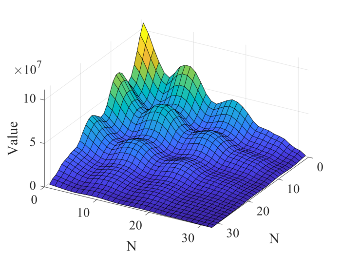
Next we examine the effect of different matrix structures on the detection performance, namely Toeplitz HPD matrices (3) and HPD matrices obtained from diagonal loading (6). Firstly, we analyze the energy distributions for these two matrix structures, shown in Fig. 7. It is observed that for the Toeplitz HPD matrix case, the energy is distributed parallel to the main diagonal and mainly distributed on the main diagonal. The farther the main diagonal is away, the less is the energy. However, for the diagonal loading HPD matrix case, the energy is mainly concentrated in a certain angle. The difference of their energy distributions is potentially one reason of their different detection performances. In Fig. 8, we analyze the performance of MIG detectors under different matrix structures. In the Gaussian clutter case, it is shown in Fig. 8 (a) that the TLD-MIG and AIRM-MIG detectors with the diagonal loading structure can achieve several performance improvements over their counterparts with the Toeplitz structure, whereas both the TSL-MIG and TVN-MIG detectors have similar performance with the diagonal loading and Toeplitz structures. In the non-Gaussian clutter case, Fig. 8 (b) shows that except for the similar performance of TSL-MIG detector, the performances of all MIG detectors with the diagonal loading structure are better to that of the detectors with the Toeplitz structure.
VI Conclusions
In this paper, we proposed a TBD-MIG detector to investigate the problem of target detection in nonhomogeneous clutter. The sample data has been assumed to be modeled as HPD matrices, which is used as the secondary data to estimate the CCM by the TBD mean. We then reformulated the problem of signal detection as discriminating two points on the HPD matrix manifold. Three TBD-MIG detectors, referred to as the TSL-MIG, TLD-MIG and TVN-MIG detectors, were introduced. Influence functions related to geometric means with respect to different divergences were defined and calculated in closed-form, providing convenience of a theoretical analysis of the robustness to outliers. Interestingly, the TBD mean is upper bounded about the interference energy. Numerical simulations shown that the TBD-MIG detectors outperform the AIRM-MIG detector and the AMF in homogeneous clutter. Energy distributions of two matrix structures, i.e., Toeplitz HPD matrices and HPD matrices obtained from diagonal loading, were analyzed, and a comparison of their influences on detection performance was also conducted.
From the theoretical aspect, it would be interesting to study the Riemannian-geometric structures induced from the proposed total divergences as well as their relations with that of the well-known AIRM and the Log-Euclidean geometry of HPD matrix manifolds [53]. Possible future research in applications will concern the target detection in real datasets using the TBD-MIG detectors and the extension of MIG detectors to the structured covariance interference, e.g., persymmetric covariance matrices [54, 55].
Appendix A Proof of Proposition 4
The following two lemmas are used in the proof of Proposition 4.
Lemma 14 ([52, 56]).
Suppose is an invertible matrix that does not have eigenvalues in the closed negative real line and denote its principal logarithm. The matrix satisfies the following properties.
- (i)
Both and commute with for any real number .
- (ii)
The following identity holds that
Lemma 15 ([56]).
- (i)
For an arbitrary matrix with and arbitrary real numbers , the following commutative property holds:
- (ii)
Suppose is an invertible matrix which does not have eigenvalues lying in the closed real line. Then, we have
Proof of Proposition 4. Denote , which is assumed to have no eigenvalues lying in the negative real line. Gradient of the function is calculated as
What left is to compute the last differentiation term. By using Lemmas 14 and 15, we have
that equals to for the matrix . Therefore, we have
and consequently and norm of the gradient is
Consequently, the Bregman divergence is given by
and hence we obtain the TVN as
Appendix B Proof of Proposition 10
Define as the objective function to be minimized for the enlarged HPD matrices, namely
The gradient of the norm function with respect to the AIRM was shown to be [56]
Consequently, we have
As is the mean of HPD matrices and outliers , then , namely
To obtain the linear term about , we can simply differentiate the equality above and then set to be zero. By doing so, we obtain
| (47) |
The condition that is the mean of HPD matrices is applied, i.e.,
References
- [1] C. D. Richmond, “Performance of a class of adaptive detection algorithms in nonhomogeneous environments,” IEEE Transactions on Signal Processing, vol. 48, no. 5, pp. 1248–1262, May 2000.
- [2] S. Deshmukh and A. Dubey, “Improved covariance matrix estimation with an application in portfolio optimization,” IEEE Signal Processing Letters, vol. 27, pp. 985–989, 2020.
- [3] A. Aubry, A. De Maio, and L. Pallotta, “A geometric approach to covariance matrix estimation and its applications to radar problems,” IEEE Transactions on Signal Processing, vol. 66, no. 4, pp. 907–922, Feb 2018.
- [4] E. J. Kelly, “An adaptive detection algorithm,” IEEE Transactions on Aerospace and Electronic Systems, vol. AES-22, no. 2, pp. 115–127, 1986.
- [5] F. C. Robey, D. R. Fuhrmann, E. J. Kelly, and R. Nitzberg, “A CFAR adaptive matched filter detector,” IEEE Transactions on Aerospace and Electronic Systems, vol. 28, no. 1, pp. 208–216, 1992.
- [6] E. Conte, M. Lops, and G. Ricci, “Adaptive matched filter detection in spherically invariant noise,” IEEE Signal Processing Letters, vol. 3, no. 8, pp. 248–250, 1996.
- [7] D. Ciuonzo, A. De Maio, and D. Orlando, “A unifying framework for adaptive radar detection in homogeneous plus structured interference–Part II: Detectors design,” IEEE Transactions on Signal Processing, vol. 64, no. 11, pp. 2907–2919, 2016.
- [8] ——, “On the statistical invariance for adaptive radar detection in partially homogeneous disturbance plus structured interference,” IEEE Transactions on Signal Processing, vol. 65, no. 5, pp. 1222–1234, 2017.
- [9] K. Ghojavand, M. Derakhtian, and M. Biguesh, “Rao-based detectors for adaptive target detection in the presence of signal-dependent interference,” IEEE Transactions on Signal Processing, vol. 68, pp. 1662–1672, 2020.
- [10] M. Li, G. Sun, J. Tong, and Z. He, “Covariance matrix whitening-based training sample selection method for airborne radar,” IEEE Geoscience and Remote Sensing Letters, pp. 1–5, 2020.
- [11] A. Aubry, A. D. Maio, L. Pallotta, and A. Farina, “Covariance matrix estimation via geometric barycenters and its application to radar training data selection,” IET Radar, Sonar & Navigation, vol. 7, no. 6, pp. 600–614, July 2013.
- [12] ——, “Median matrices and their application to radar training data selection,” IET Radar, Sonar & Navigation, vol. 8, no. 4, pp. 265–274, 2014.
- [13] P. Chen, W. L. Melvin, and M. C. Wicks, “Screening among multivariate normal data,” Journal of Multivariate Analysis, vol. 69, no. 1, pp. 10–29, 1999.
- [14] K. Gerlach, “Outlier resistant adaptive matched filtering,” IEEE Transactions on Aerospace and Electronic Systems, vol. 38, no. 3, pp. 885–901, 2002.
- [15] A. D. Maio, A. Farina, and G. Foglia, “Design and experimental validation of knowledge-based constant false alarm rate detectors,” IET Radar, Sonar & Navigation, vol. 1, no. 4, pp. 308–316, Aug 2007.
- [16] A. De Maio, A. Farina, and G. Foglia, “Knowledge-aided Bayesian radar detectors & their application to live data,” IEEE Transactions on Aerospace and Electronic Systems, vol. 46, no. 1, pp. 170–183, Jan 2010.
- [17] P. Wang, H. Li, and B. Himed, “Knowledge-aided parametric tests for multichannel adaptive signal detection,” IEEE Transactions on Signal Processing, vol. 59, no. 12, pp. 5970–5982, Dec 2011.
- [18] M. Riedl and L. C. Potter, “Knowledge-aided Bayesian space-time adaptive processing,” IEEE Transactions on Aerospace and Electronic Systems, vol. 54, no. 4, pp. 1850–1861, Aug 2018.
- [19] F. Bandiera, O. Besson, and G. Ricci, “Knowledge-aided covariance matrix estimation and adaptive detection in compound-Gaussian noise,” IEEE Transactions on Signal Processing, vol. 58, no. 10, pp. 5391–5396, Oct 2010.
- [20] O. Besson, J. Tourneret, and S. Bidon, “Knowledge-aided Bayesian detection in heterogeneous environments,” IEEE Signal Processing Letters, vol. 14, no. 5, pp. 355–358, May 2007.
- [21] C. R. Rao, Information and the Accuracy Attainable in the Estimation of Statistical Parameters. New York: Springer, 1992, pp. 235–247.
- [22] N. N. Chentsov, Statistical Decision Rules and Optimal Inference. Moscow: Nauka, 1972, in Russian.
- [23] B. Efron, “Defining the curvature of a statistical problem (with applications to second order efficiency),” Annals of Statistics, vol. 3, no. 6, pp. 1189–1242, 1975.
- [24] S. Amari, “Information geometry and the EM algorithm,” in ICANN ’94, M. Marinaro and P. G. Morasso, Eds. London: Springer, 1994, pp. 675–680.
- [25] S.-i. Amari and H. Nagaoka, Methods of Information Geometry. AMS, 2000, vol. 191.
- [26] G. Cui, N. Li, L. Pallotta, G. Foglia, and L. Kong, “Geometric barycenters for covariance estimation in compound-Gaussian clutter,” IET Radar, Sonar & Navigation, vol. 11, no. 3, pp. 404–409, 2017.
- [27] F. Barbaresco and M. Ruiz, “Radar detection for non-stationary Doppler signal in one burst based on information geometry: Distance between paths on covariance matrices manifold,” in 2015 European Radar Conference (EuRAD), Sep. 2015, pp. 41–44.
- [28] J. Lapuyade-Lahorgue and F. Barbaresco, “Radar detection using Siegel distance between autoregressive processes, application to HF and X-band radar,” in 2008 IEEE Radar Conference, May 2008, pp. 1–6.
- [29] A. Decurninge and F. Barbaresco, “Robust Burg estimation of radar scatter matrix for autoregressive structured SIRV based on fréchet medians,” IET Radar, Sonar & Navigation, vol. 11, no. 1, pp. 78–89, 2017.
- [30] F. Barbaresco, “Coding statistical characterization of radar signal fluctuation for lie group machine learning,” in 2019 International Radar Conference (RADAR), 2019, pp. 1–6.
- [31] Z. Liu and F. Barbaresco, “Doppler information geometry for wake turbulence monitoring,” in Matrix Information Geometry, F. Nielsen and R. Bhatia, Eds. Berlin, Heidelberg: Springer, 2013, pp. 277–290.
- [32] F. Barbaresco and U. Meier, “Radar monitoring of a wake vortex: Electromagnetic reflection of wake turbulence in clear air,” Comptes Rendus Physique, vol. 11, no. 1, pp. 54–67, 2010.
- [33] Y. I. Abramovich, N. K. Spencer, and A. Y. Gorokhov, “Modified GLRT and AMF framework for adaptive detectors,” IEEE Transactions on Aerospace and Electronic Systems, vol. 43, no. 3, pp. 1017–1051, 2007.
- [34] A. De Maio, L. Pallotta, J. Li, and P. Stoica, “Loading factor estimation under affine constraints on the covariance eigenvalues with application to radar target detection,” IEEE Transactions on Aerospace and Electronic Systems, vol. 55, no. 3, pp. 1269–1283, 2019.
- [35] B. D. Carlson, “Covariance matrix estimation errors and diagonal loading in adaptive arrays,” IEEE Transactions on Aerospace and Electronic Systems, vol. 24, no. 4, pp. 397–401, 1988.
- [36] L. Du, J. Li, and P. Stoica, “Fully automatic computation of diagonal loading levels for robust adaptive beamforming,” IEEE Transactions on Aerospace and Electronic Systems, vol. 46, no. 1, pp. 449–458, 2010.
- [37] X. Hua, Y. Cheng, H. Wang, Y. Qin, Y. Li, and W. Zhang, “Matrix CFAR detectors based on symmetrized Kullback–Leibler and total Kullback–Leibler divergences,” Digital Signal Processing, vol. 69, pp. 106–116, 2017.
- [38] X. Hua, Y. Cheng, H. Wang, Y. Qin, and Y. Li, “Geometric means and medians with applications to target detection,” IET Signal Processing, vol. 11, no. 6, pp. 711–720, 2017.
- [39] X. Hua, Y. Shi, Y. Zeng, C. Chen, W. Lu, Y. Cheng, and H. Wang, “A divergence mean-based geometric detector with a pre-processing procedure,” Measurement, vol. 131, pp. 640–646, 2019.
- [40] M. R. Bridson and A. Häfliger, Metric Spaces of Non-Positive Curvature. Springer Science & Business Media, 1999, vol. 319.
- [41] X. Hua, Y. Cheng, H. Wang, Y. Qin, and D. Chen, “Geometric target detection based on total Bregman divergence,” Digital Signal Processing, vol. 75, pp. 232–241, 2018.
- [42] H. Sun, Z. Zhang, L. Peng, and X. Duan, An Elementary Introduction to Information Geometry. Beijing: Science Press, 2016.
- [43] S. Kullback and R. A. Leibler, “On information and sufficiency,” The Annals of Mathematical Statistics, vol. 22, no. 1, pp. 79–86, 1951.
- [44] C. E. Shannon, “A mathematical theory of communication,” The Bell System Technical Journal, vol. 27, no. 3, pp. 379–423, 1948.
- [45] ——, “A mathematical theory of communication,” The Bell System Technical Journal, vol. 27, no. 4, pp. 623–666, 1948.
- [46] R. A. Fisher, “On the mathematical foundations of theoretical statistics,” Philosophical Transactions of the Royal Society A: Mathematical, Physical and Engineering Sciences, vol. 222, no. 594–604, pp. 309–368, 1922.
- [47] L. M. Bregman, “The relaxation method of finding the common point of convex sets and its application to the solution of problems in convex programming,” USSR Computational Mathematics and Mathematical Physics, vol. 7, no. 3, pp. 200–217, 1967.
- [48] J. Zhang, “Divergence function, duality, and convex analysis,” Neural Computation, vol. 16, no. 1, pp. 159–195, 2004.
- [49] B. C. Vemuri, M. Liu, S.-I. Amari, and F. Nielsen, “Total Bregman divergence and its applications to DTI analysis,” IEEE Transactions on Medical Imaging, vol. 30, no. 2, pp. 475–483, 2010.
- [50] M. Liu, B. C. Vemuri, S.-I. Amari, and F. Nielsen, “Total Bregman divergence and its applications to shape retrieval,” in 2010 IEEE Computer Society Conference on Computer Vision and Pattern Recognition. IEEE, 2010, pp. 3463–3468.
- [51] I. S. Dhillon and J. A. Tropp, “Matrix nearness problems with Bregman divergences,” SIAM Journal on Matrix Analysis and Applications, vol. 29, no. 4, pp. 1120–1146, 2008.
- [52] N. J. Higham, Functions of Matrices: Theory and Computation. Philadelphia: SIAM, 2008.
- [53] V. Arsigny, P. Fillard, X. Pennec, and N. Ayache, “Geometric means in a novel vector space structure on symmetric positive-definite matrices,” SIAM Journal on Matrix Analysis and Applications, vol. 29, no. 1, pp. 328–347, 2007.
- [54] D. Ciuonzo, D. Orlando, and L. Pallotta, “On the maximal invariant statistic for adaptive radar detection in partially homogeneous disturbance with persymmetric covariance,” IEEE Signal Processing Letters, vol. 23, no. 12, pp. 1830–1834, Dec 2016.
- [55] J. Zhang, Z. Wang, Z. Zhao, and Z. Nie, “Persymmetric adaptive detection with reduced-dimension approach,” IEEE Signal Processing Letters, vol. 27, pp. 563–569, March 2020.
- [56] M. Moakher, “A differential geometric approach to the geometric mean of symmetric positive-definite matrices,” SIAM Journal on Matrix Analysis and Applications, vol. 26, no. 3, pp. 735–747, 2005.